A six-wheeled omnidirectional autonomous mobile robot

December 2000 IEEE Control Systems Magazine 53

By Kevin L. Moore and Nicholas S. Flann

eople have long dreamed about vehi-cles and machines that direct them-selves. From early science-fiction

literature to the 20th-century Americancartoon The Jetsons to recent initiatives such

as the Intelligent Vehicle Highway System, theautonomous, intelligent machine (or robotic sys-tem) has been one of the holy grails of technology. Aparticularly fertile field for autonomous systems re-search is the unmanned vehicle arena. Mobile ro-bots have been developed that can operateautonomously in underwater environments as wellas in air and outer space. Recently there has been in-creased interest in unmanned ground vehicles, orUGVs, especially for use in the military, agriculture,and civilian transportation. Today, advances in me-chanical design capabilities, sensing technologiessuch as GPS (global positioning system), computingpower and miniature electronics, and intelligent al-

Moore ([email protected]) and Flann are with the Center for Self-Organizing and Intelligent Systems, Utah State University, Logan, UT84322, U.S.A. An earlier version of this paper appeared in the Proceedings of the 1999 IEEE International Symposium on Intelligent Con-trol/Intelligent Systems and Semiotics.

0272-1708/00/$10.00©2000IEEE

gorithms for planning and control have led to the possibilityof realizing true autonomous mobile robot operation forUGV applications.

In this article we describe a specific autonomous mobilerobot developed for UGV applications. We focus on a novelrobotic platform [1], the Utah State University (USU)omnidirectional vehicle (ODV). This platform features mul-tiple “smart wheels” in which each wheel’s speed and direc -tion can be independently controlled through dedicatedprocessors. The result is a robot with the ability to com-pletely control both the vehicle’s orientation and its motionin a plane—in effect, a “hovercraft on wheels.”

We begin by describing the mobility capability inherentin the smart wheel concept and discussing the distrib-uted-processor mechatronic implementation of the com-plete system. Then we focus on a multiresolutionbehavior-generation strategy that we have developed forcontrolling the robot. The strategy is characterized by a hi-erarchical task decomposition approach. At the supervi-sory level, a knowledge-based planner and an A*-optimiza-tion algorithm are used to specify the vehicle’s path as a se-quence of basic maneuvers. At the vehicle level, these basicmaneuvers are converted to time-domain trajectories.These trajectories are then tracked in an inertial referenceframe using a model-based feedback linearization control-ler that computes set points for each wheel’s low-level drivemotor and steering angle motor controllers. The effective-ness of the strategy is demonstrated by results from actualtests with several real robots designed using the smartwheel concept.

The USU ODV Robotic PlatformMobility Capability and Mobility ControlMuch of the research described here was funded by the U.S.Army Tank-Automotive and Armament Command’s Intelli-gent Mobility Program. The broad objective of the program

has been to develop and demonstrate intelligent mobilityconcepts for unmanned ground vehicles. Mobility means,literally, “the ability or readiness to move or be moved; be -ing mobile” [2]. Intelligent mobility adds the capability todetermine optimal paths through terrain by using varioussmart or intelligent navigation and path-planning strategies(e.g., obstacle avoidance and negotiation using cost func-tions and tradeoff analyses). Thus, in the context of autono-mous mobile robotics, we consider two components ofintelligent mobility: mobility capability and mobility control.Mobility capability refers to the physical characteristics ofthe vehicle that make it able to move. Mobility controlmeans using “intelligence” in controlling the vehicle to actu -ally achieve its full mobility capability. Mobility control alsohas two components:

• First, to manage the “local” dynamic interactions be -tween the vehicle and the forces it encounters, intelli-gent vehicle-level control algorithms must be devel-oped and implemented to optimally maneuver thevehicle.

• Second, mission mobility and path planning is con-cerned with “global” motion planning and naviga -tion and is used to determine the path a vehicleshould take to pass through a given region toachieve its objective.

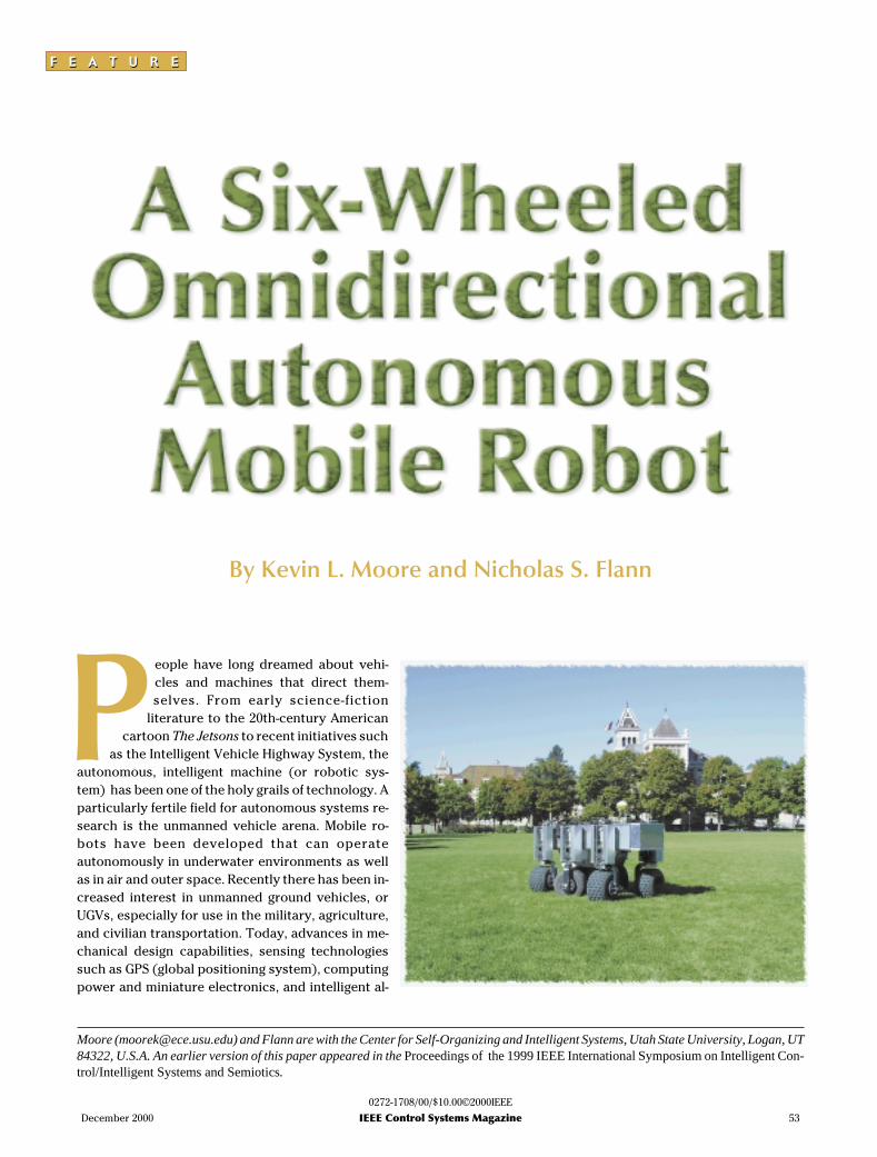
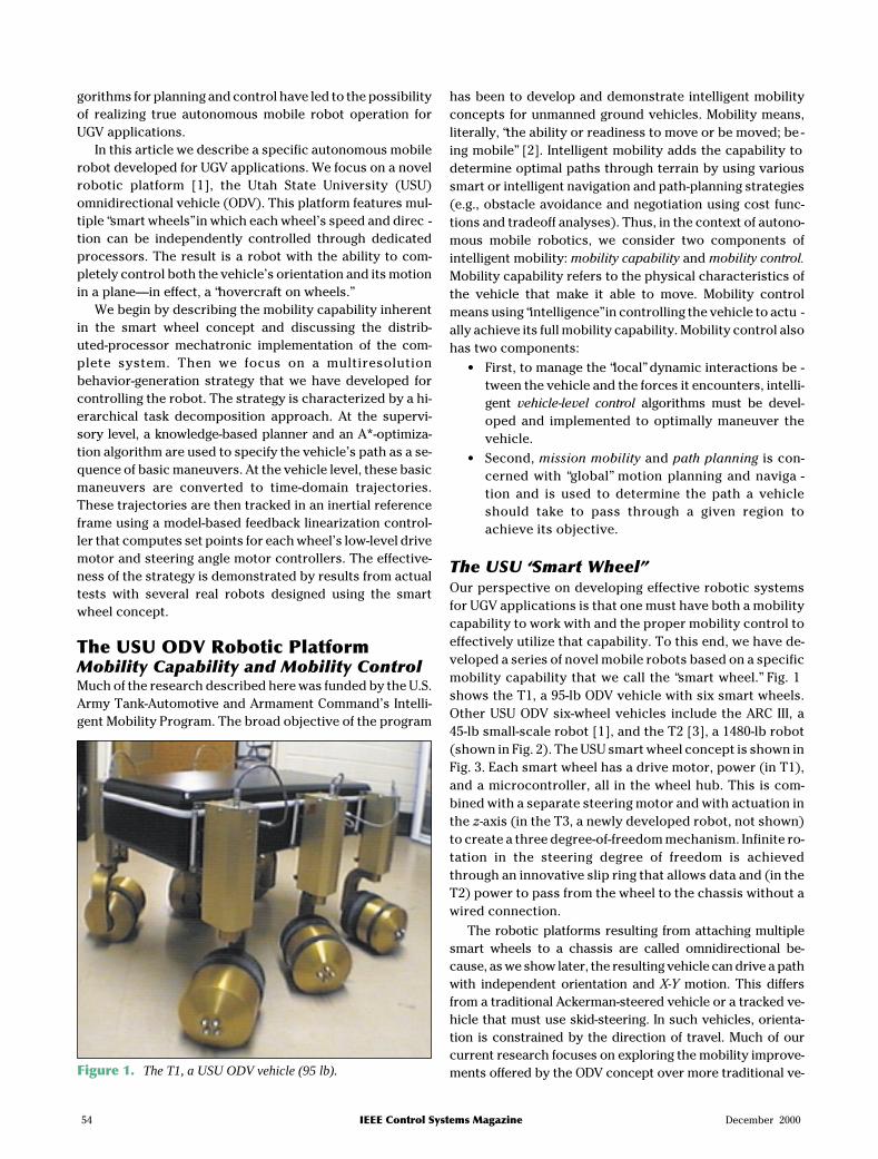
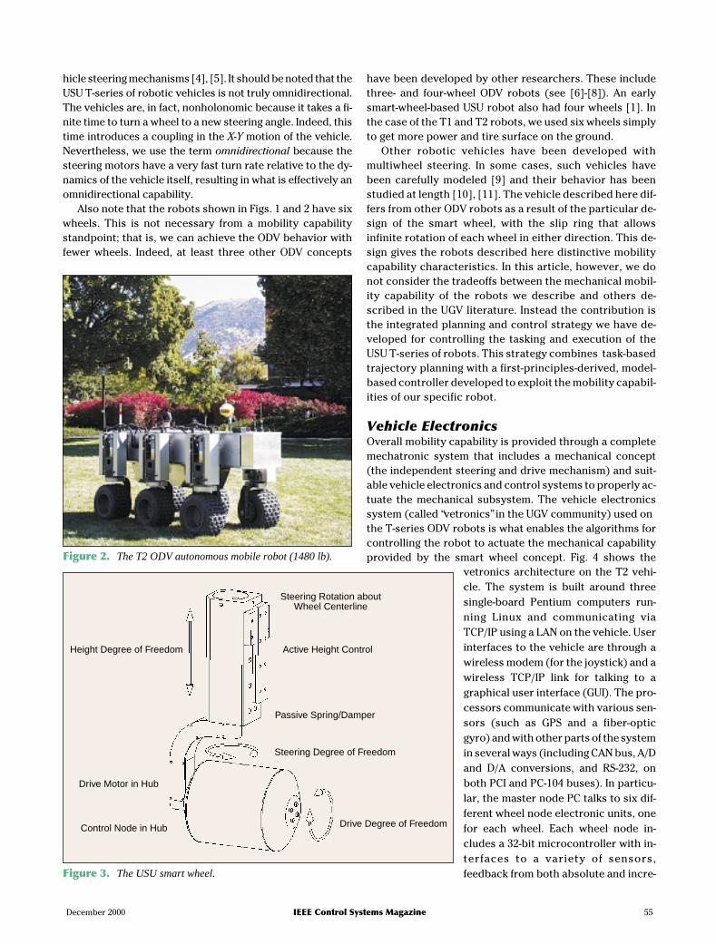
The USU “Smart Wheel”Our perspective on developing effective robotic systemsfor UGV applications is that one must have both a mobilitycapability to work with and the proper mobility control toeffectively utilize that capability. To this end, we have de-veloped a series of novel mobile robots based on a specificmobility capability that we call the “smart wheel.” Fig. 1shows the T1, a 95-lb ODV vehicle with six smart wheels.Other USU ODV six-wheel vehicles include the ARC III, a45-lb small-scale robot [1], and the T2 [3], a 1480-lb robot(shown in Fig. 2). The USU smart wheel concept is shown inFig. 3. Each smart wheel has a drive motor, power (in T1),and a microcontroller, all in the wheel hub. This is com-bined with a separate steering motor and with actuation inthe z-axis (in the T3, a newly developed robot, not shown)to create a three degree-of-freedom mechanism. Infinite ro-tation in the steering degree of freedom is achievedthrough an innovative slip ring that allows data and (in theT2) power to pass from the wheel to the chassis without awired connection.

The robotic platforms resulting from attaching multiplesmart wheels to a chassis are called omnidirectional be-cause, as we show later, the resulting vehicle can drive a pathwith independent orientation and X-Y motion. This differsfrom a traditional Ackerman-steered vehicle or a tracked ve-hicle that must use skid-steering. In such vehicles, orienta-tion is constrained by the direction of travel. Much of ourcurrent research focuses on exploring the mobility improve-ments offered by the ODV concept over more traditional ve-

54 IEEE Control Systems Magazine December 2000

Figure 1. The T1, a USU ODV vehicle (95 lb).

hicle steering mechanisms [4], [5]. It should be noted that theUSU T-series of robotic vehicles is not truly omnidirectional.The vehicles are, in fact, nonholonomic because it takes a fi-nite time to turn a wheel to a new steering angle. Indeed, thistime introduces a coupling in the X-Y motion of the vehicle.Nevertheless, we use the term omnidirectional because thesteering motors have a very fast turn rate relative to the dy-namics of the vehicle itself, resulting in what is effectively anomnidirectional capability.

Also note that the robots shown in Figs. 1 and 2 have sixwheels. This is not necessary from a mobility capabilitystandpoint; that is, we can achieve the ODV behavior withfewer wheels. Indeed, at least three other ODV concepts

have been developed by other researchers. These includethree- and four-wheel ODV robots (see [6]-[8]). An earlysmart-wheel-based USU robot also had four wheels [1]. Inthe case of the T1 and T2 robots, we used six wheels simplyto get more power and tire surface on the ground.

Other robotic vehicles have been developed withmultiwheel steering. In some cases, such vehicles havebeen carefully modeled [9] and their behavior has beenstudied at length [10], [11]. The vehicle described here dif-fers from other ODV robots as a result of the particular de-sign of the smart wheel, with the slip ring that allowsinfinite rotation of each wheel in either direction. This de-sign gives the robots described here distinctive mobilitycapability characteristics. In this article, however, we donot consider the tradeoffs between the mechanical mobil-ity capability of the robots we describe and others de-scribed in the UGV literature. Instead the contribution isthe integrated planning and control strategy we have de-veloped for controlling the tasking and execution of theUSU T-series of robots. This strategy combines task-basedtrajectory planning with a first-principles-derived, model-based controller developed to exploit the mobility capabil-ities of our specific robot.

Vehicle ElectronicsOverall mobility capability is provided through a completemechatronic system that includes a mechanical concept(the independent steering and drive mechanism) and suit-able vehicle electronics and control systems to properly ac-tuate the mechanical subsystem. The vehicle electronicssystem (called “vetronics” in the UGV community) used onthe T-series ODV robots is what enables the algorithms forcontrolling the robot to actuate the mechanical capabilityprovided by the smart wheel concept. Fig. 4 shows the

vetronics architecture on the T2 vehi-cle. The system is built around threesingle-board Pentium computers run-ning Linux and communicating viaTCP/IP using a LAN on the vehicle. Userinterfaces to the vehicle are through awireless modem (for the joystick) and awireless TCP/IP link for talking to agraphical user interface (GUI). The pro-cessors communicate with various sen-sors (such as GPS and a fiber-opticgyro) and with other parts of the systemin several ways (including CAN bus, A/Dand D/A conversions, and RS-232, onboth PCI and PC-104 buses). In particu-lar, the master node PC talks to six dif-ferent wheel node electronic units, onefor each wheel. Each wheel node in-cludes a 32-bit microcontroller with in-terfaces to a variety of sensors,feedback from both absolute and incre-


Figure 2. The T2 ODV autonomous mobile robot (1480 lb).

Drive Degree of Freedom

Height Degree of Freedom

Steering Degree of Freedom

Drive Motor in Hub

Active Height Control

Passive Spring/Damper

Control Node in Hub

Steering Rotation aboutWheel Centerline

Figure 3. The USU smart wheel.

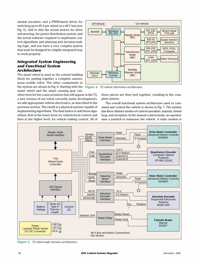
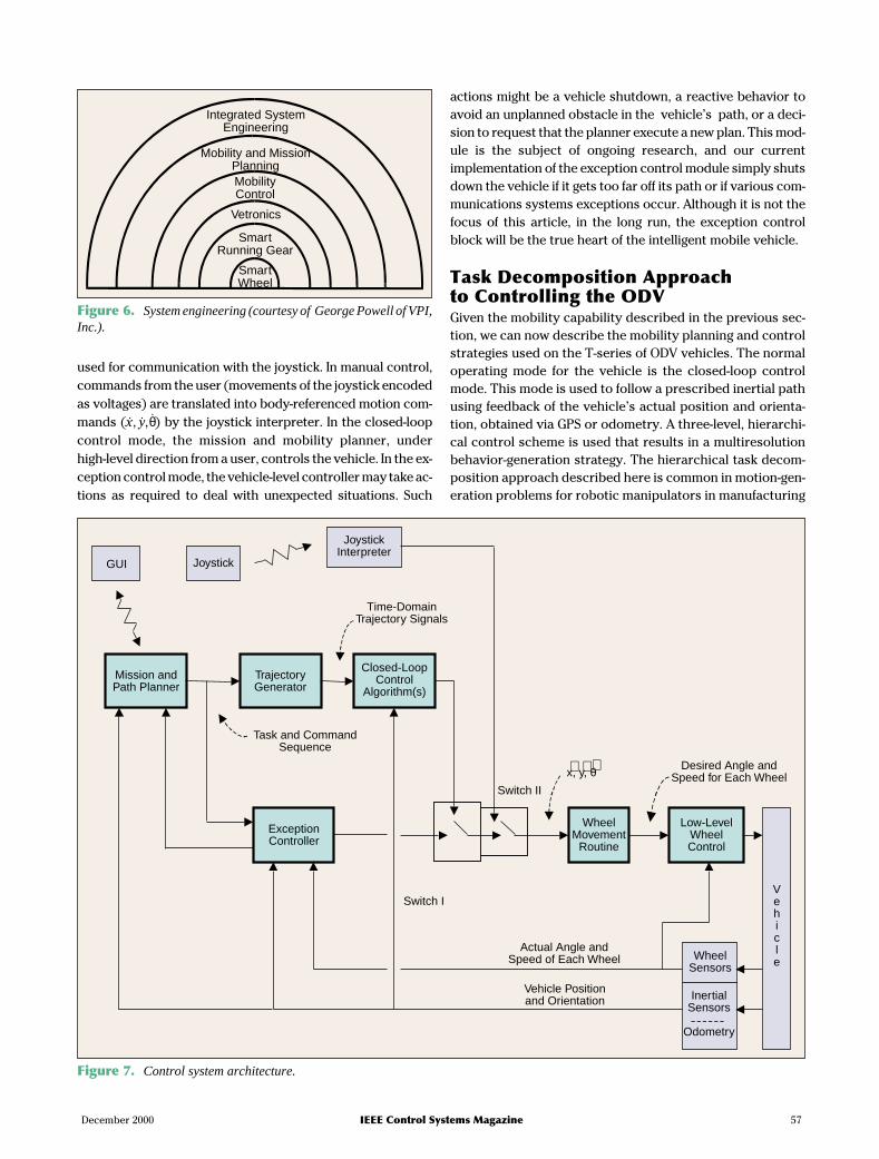
mental encoders, and a PWM-based driver forswitching up to 60 A per wheel on a 48 V bus (seeFig. 5). Add to this the actual motors for driveand steering, the power distribution system, andthe actual software required to implement con-trol algorithms and planning and decision-mak-ing logic, and you have a very complex systemthat must be designed in a highly integrated wayto work properly.

Integrated System Engineeringand Functional SystemArchitectureThe smart wheel is used as the central buildingblock for putting together a complete autono-mous mobile robot. The other components inthe system are shown in Fig. 6. Starting with thesmart wheel and the smart running gear (an-other term for the z-axis actuation that will appear in the T3,a new version of our robot currently under development),we add appropriate vehicle electronics, as described in theprevious section. The result is a physical system capable ofimplementing algorithms. The final task is to add these algo-rithms, first at the lower level, for vehicle-level control, andthen at the higher level, for vehicle tasking control. All of

these pieces are then tied together, resulting in the com-plete system.

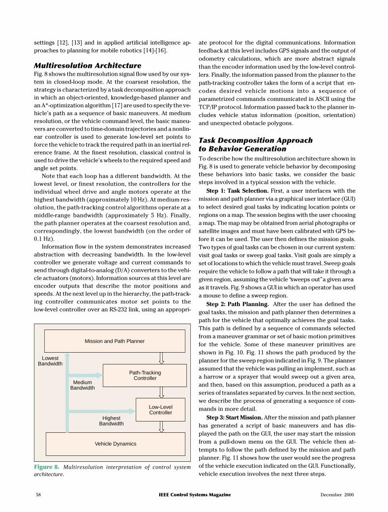
The overall functional system architecture used to com-mand and control the vehicle is shown in Fig. 7. The systemhas three distinct modes of control operation: manual, closedloop, and exception. In the manual control mode, an operatoruses a joystick to maneuver the vehicle. A radio modem is


Master NodeSBC

Nav/SensorNodeSBC

MobilityPlanner Node

SBC

RS-232(PC 104)

GPS, FOG,Compass

Other Sensors

Wheel NodeTT8 (x6)

RS-232(PCI)

CAN(PC 104)

LAN

WirelessRS-232

WirelessTCP/IP

Joystick

RemoteOCU

Off-Vehicle On-Vehicle

A/D IO(PC104)

System MonitorSensors

Figure 4. T2 vehicle electronics architecture.

Master NodeSerial Interface

TT8Wheel Node

Controller

Drive MotorInterface

SteeringMotor

Interface

QuadratureEncoderInterface

AbsoluteEncoderInterface

DPWM

SPWM

DDIR

SDIR

Dfault

Sfault

PWM

PWM

Direction

Direction

Fault

Fault

D-Current

S-Current

Drive Motor ControllerAdvanced Motion Controls

50A8DD

Steer Motor ControllerAdvanced Motion Controls

50A8DD

Quadrature EncoderComputer Optical

ProductsCP-560 (1024)

Absolute EncoderSequential Electronic

SystemsModel 40H

CHACHB

+12 V12 V ReturnChannel AChannel B

Position10

ACLKADATA

AENALBE

+5 V5 V Return

BRAKE OFF Brake Power

Power GndBrake RelayFailsafe Brake

WarnerERS57

48 V Bus and Motor ConnectionsNot Shown

A/D SignalInterface

BatteryVoltage

Temp (2)Type K

Thermo-couple

Current(2)

PowerLambda PM30 Series

DC-DC Converter

+12 V–12 V+5 V

Figure 5. T2 wheel node vetronics architecture.

used for communication with the joystick. In manual control,commands from the user (movements of the joystick encodedas voltages) are translated into body-referenced motion com-mands ( �, �, �x y θ) by the joystick interpreter. In the closed-loopcontrol mode, the mission and mobility planner, underhigh-level direction from a user, controls the vehicle. In the ex-ception control mode, the vehicle-level controller may take ac-tions as required to deal with unexpected situations. Such

actions might be a vehicle shutdown, a reactive behavior toavoid an unplanned obstacle in the vehicle’s path, or a deci-sion to request that the planner execute a new plan. This mod-ule is the subject of ongoing research, and our currentimplementation of the exception control module simply shutsdown the vehicle if it gets too far off its path or if various com-munications systems exceptions occur. Although it is not thefocus of this article, in the long run, the exception controlblock will be the true heart of the intelligent mobile vehicle.

Task Decomposition Approachto Controlling the ODVGiven the mobility capability described in the previous sec-tion, we can now describe the mobility planning and controlstrategies used on the T-series of ODV vehicles. The normaloperating mode for the vehicle is the closed-loop controlmode. This mode is used to follow a prescribed inertial pathusing feedback of the vehicle’s actual position and orienta-tion, obtained via GPS or odometry. A three-level, hierarchi-cal control scheme is used that results in a multiresolutionbehavior-generation strategy. The hierarchical task decom-position approach described here is common in motion-gen-eration problems for robotic manipulators in manufacturing


Integrated SystemEngineering

Mobility and MissionPlanningMobilityControl

Vetronics

SmartRunning Gear

SmartWheel

Figure 6. System engineering (courtesy of George Powell of VPI,Inc.).

GUI Joystick

JoystickInterpreter

Mission andPath Planner

TrajectoryGenerator

Time-DomainTrajectory Signals

Closed-LoopControl

Algorithm(s)

Task and CommandSequence

ExceptionController

Switch I

Switch II

WheelMovement

Routine

Desired Angle andSpeed for Each Wheel

Low-LevelWheelControl

Vehicle

Actual Angle andSpeed of Each Wheel

Vehicle Positionand Orientation

WheelSensors

InertialSensors

Odometry

x, y, θ⋅ ⋅ ⋅

Figure 7. Control system architecture.

settings [12], [13] and in applied artificial intelligence ap-proaches to planning for mobile robotics [14]-[16].

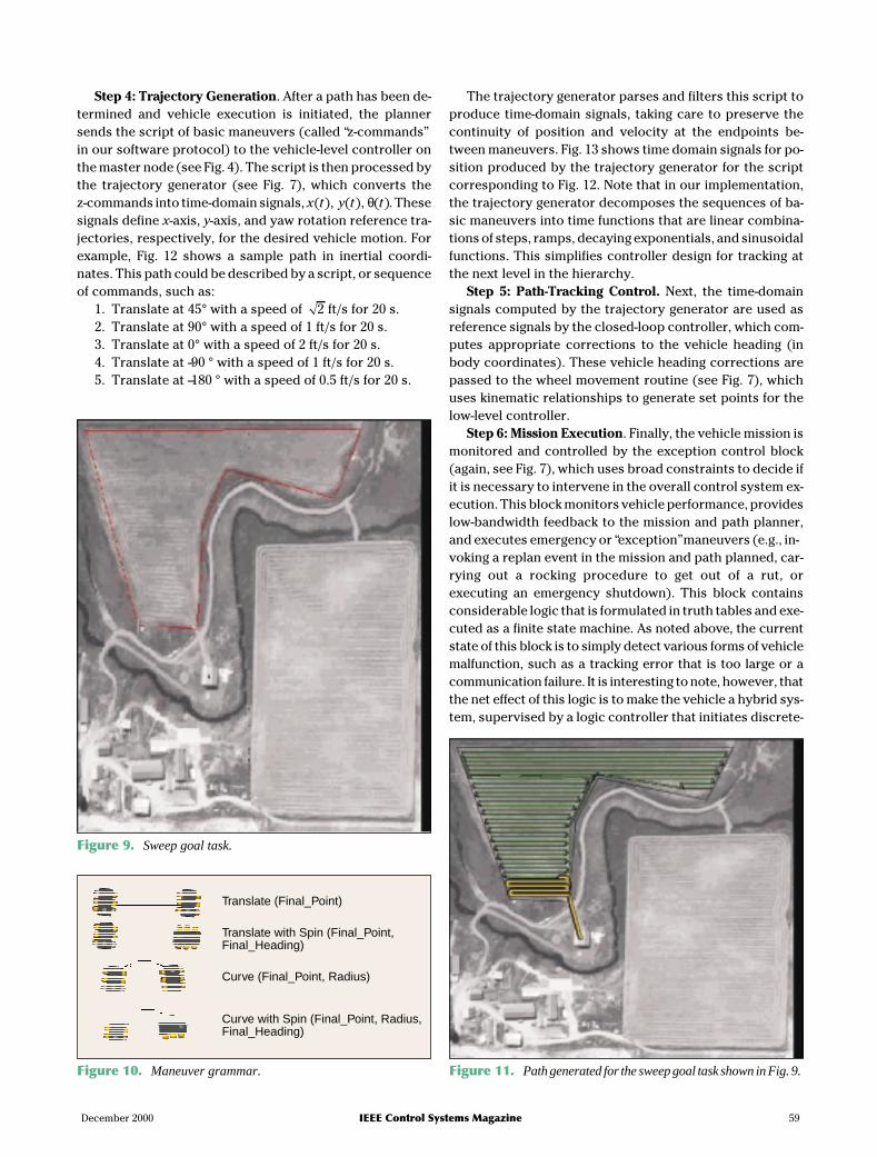
Multiresolution ArchitectureFig. 8 shows the multiresolution signal flow used by our sys-tem in closed-loop mode. At the coarsest resolution, thestrategy is characterized by a task decomposition approachin which an object-oriented, knowledge-based planner andan A*-optimization algorithm [17] are used to specify the ve-hicle’s path as a sequence of basic maneuvers. At mediumresolution, or the vehicle command level, the basic maneu-vers are converted to time-domain trajectories and a nonlin-ear controller is used to generate low-level set points toforce the vehicle to track the required path in an inertial ref-erence frame. At the finest resolution, classical control isused to drive the vehicle’s wheels to the required speed andangle set points.

Note that each loop has a different bandwidth. At thelowest level, or finest resolution, the controllers for theindividual wheel drive and angle motors operate at thehighest bandwidth (approximately 10 Hz). At medium res-olution, the path-tracking control algorithms operate at amiddle-range bandwidth (approximately 5 Hz). Finally,the path planner operates at the coarsest resolution and,correspondingly, the lowest bandwidth (on the order of0.1 Hz).

Information flow in the system demonstrates increasedabstraction with decreasing bandwidth. In the low-levelcontroller we generate voltage and current commands tosend through digital-to-analog (D/A) converters to the vehi-cle actuators (motors). Information sources at this level areencoder outputs that describe the motor positions andspeeds. At the next level up in the hierarchy, the path-track-ing controller communicates motor set points to thelow-level controller over an RS-232 link, using an appropri-

ate protocol for the digital communications. Informationfeedback at this level includes GPS signals and the output ofodometry calculations, which are more abstract signalsthan the encoder information used by the low-level control-lers. Finally, the information passed from the planner to thepath-tracking controller takes the form of a script that en-codes desired vehicle motions into a sequence ofparametrized commands communicated in ASCII using theTCP/IP protocol. Information passed back to the planner in-cludes vehicle status information (position, orientation)and unexpected obstacle polygons.

Task Decomposition Approachto Behavior GenerationTo describe how the multiresolution architecture shown inFig. 8 is used to generate vehicle behavior by decomposingthese behaviors into basic tasks, we consider the basicsteps involved in a typical session with the vehicle.

Step 1: Task Selection. First, a user interfaces with themission and path planner via a graphical user interface (GUI)to select desired goal tasks by indicating location points orregions on a map. The session begins with the user choosinga map. The map may be obtained from aerial photographs orsatellite images and must have been calibrated with GPS be-fore it can be used. The user then defines the mission goals.Two types of goal tasks can be chosen in our current system:visit goal tasks or sweep goal tasks. Visit goals are simply aset of locations to which the vehicle must travel. Sweep goalsrequire the vehicle to follow a path that will take it through agiven region, assuming the vehicle “sweeps out” a given areaas it travels. Fig. 9 shows a GUI in which an operator has useda mouse to define a sweep region.

Step 2: Path Planning. After the user has defined thegoal tasks, the mission and path planner then determines apath for the vehicle that optimally achieves the goal tasks.This path is defined by a sequence of commands selectedfrom a maneuver grammar or set of basic motion primitivesfor the vehicle. Some of these maneuver primitives areshown in Fig. 10. Fig. 11 shows the path produced by theplanner for the sweep region indicated in Fig. 9. The plannerassumed that the vehicle was pulling an implement, such asa harrow or a sprayer that would sweep out a given area,and then, based on this assumption, produced a path as aseries of translates separated by curves. In the next section,we describe the process of generating a sequence of com-mands in more detail.

Step 3: Start Mission. After the mission and path plannerhas generated a script of basic maneuvers and has dis-played the path on the GUI, the user may start the missionfrom a pull-down menu on the GUI. The vehicle then at-tempts to follow the path defined by the mission and pathplanner. Fig. 11 shows how the user would see the progressof the vehicle execution indicated on the GUI. Functionally,vehicle execution involves the next three steps.


Mission and Path Planner

Path-TrackingController

Low-LevelController

Vehicle Dynamics

LowestBandwidth

MediumBandwidth

HighestBandwidth

Figure 8. Multiresolution interpretation of control systemarchitecture.

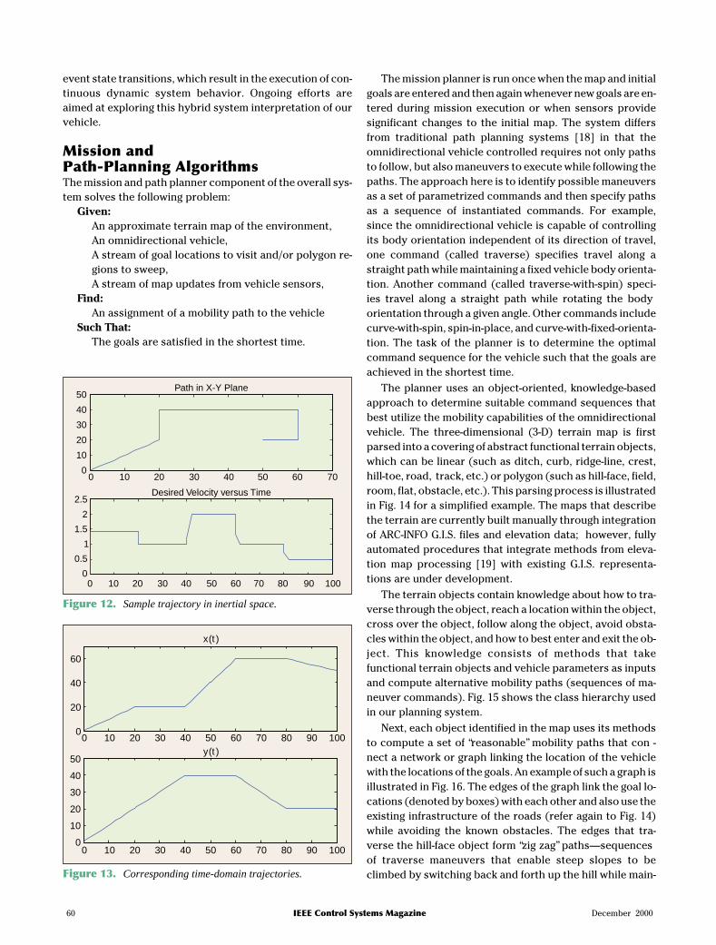
Step 4: Trajectory Generation. After a path has been de-termined and vehicle execution is initiated, the plannersends the script of basic maneuvers (called “z-commands”in our software protocol) to the vehicle-level controller onthe master node (see Fig. 4). The script is then processed bythe trajectory generator (see Fig. 7), which converts thez-commands into time-domain signals, x t y t t( ), ( ), ( )θ . Thesesignals define x-axis, y-axis, and yaw rotation reference tra-jectories, respectively, for the desired vehicle motion. Forexample, Fig. 12 shows a sample path in inertial coordi-nates. This path could be described by a script, or sequenceof commands, such as:

1. Translate at 45° with a speed of 2 ft/s for 20 s.2. Translate at 90° with a speed of 1 ft/s for 20 s.3. Translate at 0° with a speed of 2 ft/s for 20 s.4. Translate at –90 ° with a speed of 1 ft/s for 20 s.5. Translate at –180 ° with a speed of 0.5 ft/s for 20 s.

The trajectory generator parses and filters this script toproduce time-domain signals, taking care to preserve thecontinuity of position and velocity at the endpoints be-tween maneuvers. Fig. 13 shows time domain signals for po-sition produced by the trajectory generator for the scriptcorresponding to Fig. 12. Note that in our implementation,the trajectory generator decomposes the sequences of ba-sic maneuvers into time functions that are linear combina-tions of steps, ramps, decaying exponentials, and sinusoidalfunctions. This simplifies controller design for tracking atthe next level in the hierarchy.

Step 5: Path-Tracking Control. Next, the time-domainsignals computed by the trajectory generator are used asreference signals by the closed-loop controller, which com-putes appropriate corrections to the vehicle heading (inbody coordinates). These vehicle heading corrections arepassed to the wheel movement routine (see Fig. 7), whichuses kinematic relationships to generate set points for thelow-level controller.

Step 6: Mission Execution. Finally, the vehicle mission ismonitored and controlled by the exception control block(again, see Fig. 7), which uses broad constraints to decide ifit is necessary to intervene in the overall control system ex-ecution. This block monitors vehicle performance, provideslow-bandwidth feedback to the mission and path planner,and executes emergency or “exception” maneuvers (e.g., in-voking a replan event in the mission and path planned, car-rying out a rocking procedure to get out of a rut, orexecuting an emergency shutdown). This block containsconsiderable logic that is formulated in truth tables and exe-cuted as a finite state machine. As noted above, the currentstate of this block is to simply detect various forms of vehiclemalfunction, such as a tracking error that is too large or acommunication failure. It is interesting to note, however, thatthe net effect of this logic is to make the vehicle a hybrid sys-tem, supervised by a logic controller that initiates discrete-


Figure 9. Sweep goal task.

Translate (Final_Point)

Translate with Spin (Final_Point,Final_Heading)

Curve (Final_Point, Radius)

Curve with Spin (Final_Point, Radius,Final_Heading)

Figure 10. Maneuver grammar. Figure 11. Path generated for the sweep goal task shown in Fig. 9.

event state transitions, which result in the execution of con-tinuous dynamic system behavior. Ongoing efforts areaimed at exploring this hybrid system interpretation of ourvehicle.

Mission andPath-Planning AlgorithmsThe mission and path planner component of the overall sys-tem solves the following problem:

Given:An approximate terrain map of the environment,An omnidirectional vehicle,A stream of goal locations to visit and/or polygon re-gions to sweep,A stream of map updates from vehicle sensors,

Find:An assignment of a mobility path to the vehicle

Such That:The goals are satisfied in the shortest time.

The mission planner is run once when the map and initialgoals are entered and then again whenever new goals are en-tered during mission execution or when sensors providesignificant changes to the initial map. The system differsfrom traditional path planning systems [18] in that theomnidirectional vehicle controlled requires not only pathsto follow, but also maneuvers to execute while following thepaths. The approach here is to identify possible maneuversas a set of parametrized commands and then specify pathsas a sequence of instantiated commands. For example,since the omnidirectional vehicle is capable of controllingits body orientation independent of its direction of travel,one command (called traverse) specifies travel along astraight path while maintaining a fixed vehicle body orienta-tion. Another command (called traverse-with-spin) speci-ies travel along a straight path while rotating the bodyorientation through a given angle. Other commands includecurve-with-spin, spin-in-place, and curve-with-fixed-orienta-tion. The task of the planner is to determine the optimalcommand sequence for the vehicle such that the goals areachieved in the shortest time.

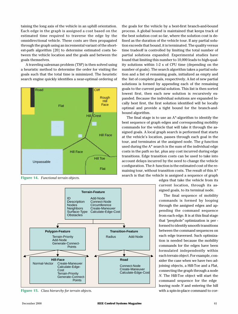
The planner uses an object-oriented, knowledge-basedapproach to determine suitable command sequences thatbest utilize the mobility capabilities of the omnidirectionalvehicle. The three-dimensional (3-D) terrain map is firstparsed into a covering of abstract functional terrain objects,which can be linear (such as ditch, curb, ridge-line, crest,hill-toe, road, track, etc.) or polygon (such as hill-face, field,room, flat, obstacle, etc.). This parsing process is illustratedin Fig. 14 for a simplified example. The maps that describethe terrain are currently built manually through integrationof ARC-INFO G.I.S. files and elevation data; however, fullyautomated procedures that integrate methods from eleva-tion map processing [19] with existing G.I.S. representa-tions are under development.

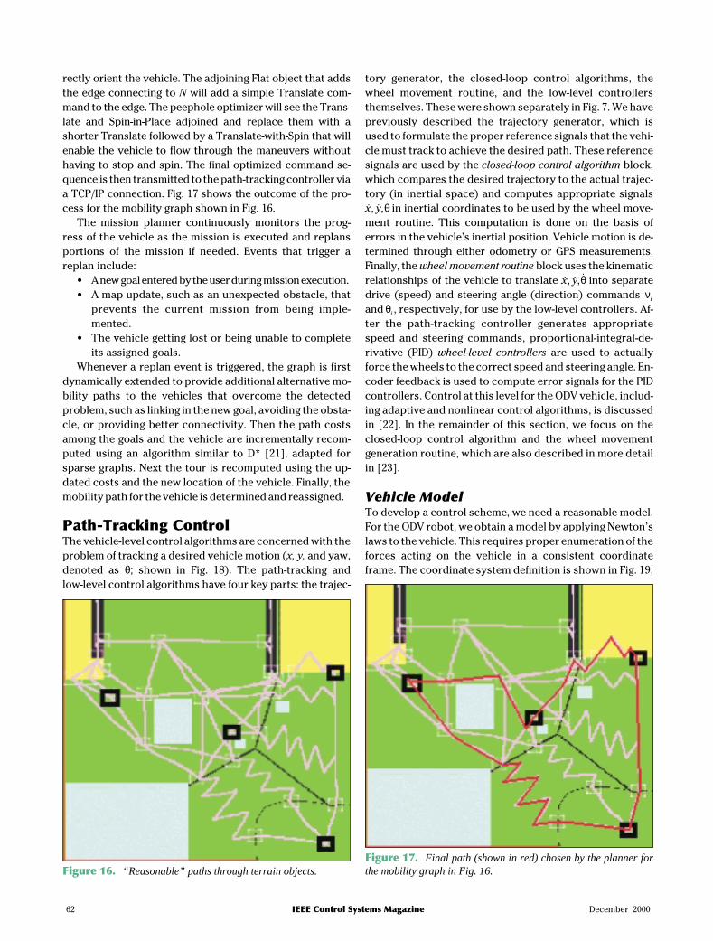
The terrain objects contain knowledge about how to tra-verse through the object, reach a location within the object,cross over the object, follow along the object, avoid obsta-cles within the object, and how to best enter and exit the ob-ject. This knowledge consists of methods that takefunctional terrain objects and vehicle parameters as inputsand compute alternative mobility paths (sequences of ma-neuver commands). Fig. 15 shows the class hierarchy usedin our planning system.

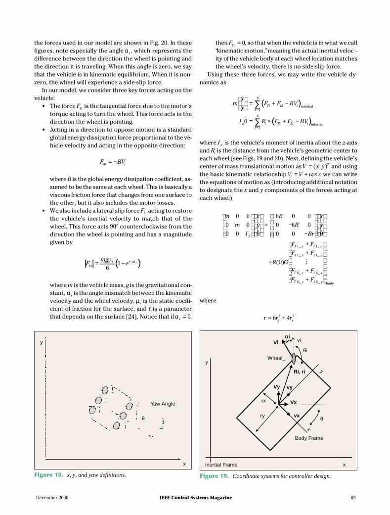
Next, each object identified in the map uses its methodsto compute a set of “reasonable” mobility paths that con -nect a network or graph linking the location of the vehiclewith the locations of the goals. An example of such a graph isillustrated in Fig. 16. The edges of the graph link the goal lo-cations (denoted by boxes) with each other and also use theexisting infrastructure of the roads (refer again to Fig. 14)while avoiding the known obstacles. The edges that tra-verse the hill-face object form “zig zag” paths—sequencesof traverse maneuvers that enable steep slopes to beclimbed by switching back and forth up the hill while main-


50Path in X-Y Plane

Desired Velocity versus Time

40

30

20

10

0

2.5

2

1.5

1

0.5

0

0 10 20 30 40 50 60 70

0 10 20 30 40 50 60 70 80 90 100

Figure 12. Sample trajectory in inertial space.

0

0

10

10

20

20

30

30

40

40

50

50

60

60

70

70

80

80

90

90

100

100

0

20

40

60

50

40

30

20

10

0

x t( )

y t( )

Figure 13. Corresponding time-domain trajectories.

taining the long axis of the vehicle in an uphill orientation.Each edge in the graph is assigned a cost based on theestimated time required to traverse the edge by theomnidirectional vehicle. These costs are then propagatedthrough the graph using an incremental variant of the short-est-path algorithm [20] to determine estimated costs be-tween the vehicle location and the goals and between thegoals themselves.

A traveling salesman problem (TSP) is then solved usinga heuristic method to determine the order for visiting thegoals such that the total time is minimized. The heuristicsearch engine quickly identifies a near-optimal ordering of

the goals for the vehicle by a best-first branch-and-boundprocess. A global bound is maintained that keeps track ofthe best solution cost so far, where the solution cost is de-fined as the duration of the vehicle tour. If any partial solu-tion exceeds that bound, it is terminated. The quality versustime tradeoff is controlled by limiting the total number ofpartial solutions expanded. Experimental studies havefound that limiting this number to 10,000 leads to high-qual-ity solutions within 1-2 s of CPU time (depending on thenumber of goals). The search algorithm takes a partial solu-tion and a list of remaining goals, initialized as empty andthe list of complete goals, respectively. A list of new partialsolutions is formed by appending each of the remaininggoals to the current partial solution. This list is then sortedlowest first, then each new solution is recursively ex-panded. Because the individual solutions are expanded lo-cally best first, the first solution identified will be locallyoptimal and provide a tight bound for the branch-and-bound algorithm.

The final stage is to use an A*-algorithm to identify thebest sequence of graph edges and corresponding mobilitycommands for the vehicle that will take it through the as-signed goals. A local graph search is performed that startsat the vehicle’s location, passes through each goal in thetour, and terminates at the assigned node. The g functionused during the A* search is the sum of the individual edgecosts in the path so far, plus any cost incurred during edgetransitions. Edge transition costs can be used to take intoaccount delays incurred by the need to change the vehicleconfiguration. The h function is the estimated cost of the re-maining tour, without transition costs. The result of this A*search is that the vehicle is assigned a sequence of graph

edges that take the vehicle from itscurrent location, through its as-signed goals, to its terminal node.

The final sequence of mobilitycommands is formed by loopingthrough the assigned edges and ap-pending the command sequencefrom each edge. It is at this final stagethat “peephole” optimization is per -formed to identify smooth transitionsbetween the command sequences oneach edge traversed. Such optimiza-tion is needed because the mobilitycommands for the edges have beenformulated independently withineach terrain object. For example, con-sider the case when we have two ad-joining objects, a Hill-Toe and a Flat,connecting the graph through a nodeN. The Hill-Toe object will start thecommand sequence for the edgeleaving node N and entering the hillwith a spin-in-place command to cor-


Flat

Road

RoughHill

Face

Cliff

Hill Crest

Hill Face

Hill Face

Flat

Hill ToeUnpassable

Figure 14. Functional terrain objects.

Terrain-Feature

IDDescriptionNodesNeighborsSurface-TypeObstacles

Add-NodeConnect-NodeCircumferenceCreate-ManeuverCalculate-Edge-Cost

Polygon-Feature

Terrain-PriorityAdd-NodeGenerate-Connect-

Points

Transition-Feature

Radius Add-Node

Hill-FaceNormal-Vector Create-Maneuver

Calculate-Edge-CostTerrain-PriorityGenerate-Connect-

Points

Road

Connect-NodeCreate-ManeuverCalculate-Edge-Cost

Figure 15. Class hierarchy for terrain objects.

rectly orient the vehicle. The adjoining Flat object that addsthe edge connecting to N will add a simple Translate com-mand to the edge. The peephole optimizer will see the Trans-late and Spin-in-Place adjoined and replace them with ashorter Translate followed by a Translate-with-Spin that willenable the vehicle to flow through the maneuvers withouthaving to stop and spin. The final optimized command se-quence is then transmitted to the path-tracking controller viaa TCP/IP connection. Fig. 17 shows the outcome of the pro-cess for the mobility graph shown in Fig. 16.

The mission planner continuously monitors the prog-ress of the vehicle as the mission is executed and replansportions of the mission if needed. Events that trigger areplan include:

• Anewgoalenteredbytheuserduringmissionexecution.• A map update, such as an unexpected obstacle, that

prevents the current mission from being imple-mented.

• The vehicle getting lost or being unable to completeits assigned goals.

Whenever a replan event is triggered, the graph is firstdynamically extended to provide additional alternative mo-bility paths to the vehicles that overcome the detectedproblem, such as linking in the new goal, avoiding the obsta-cle, or providing better connectivity. Then the path costsamong the goals and the vehicle are incrementally recom-puted using an algorithm similar to D* [21], adapted forsparse graphs. Next the tour is recomputed using the up-dated costs and the new location of the vehicle. Finally, themobility path for the vehicle is determined and reassigned.

Path-Tracking ControlThe vehicle-level control algorithms are concerned with theproblem of tracking a desired vehicle motion (x, y, and yaw,denoted as θ; shown in Fig. 18). The path-tracking andlow-level control algorithms have four key parts: the trajec-

tory generator, the closed-loop control algorithms, thewheel movement routine, and the low-level controllersthemselves. These were shown separately in Fig. 7. We havepreviously described the trajectory generator, which isused to formulate the proper reference signals that the vehi-cle must track to achieve the desired path. These referencesignals are used by the closed-loop control algorithm block,which compares the desired trajectory to the actual trajec-tory (in inertial space) and computes appropriate signals�, �, �x y θ in inertial coordinates to be used by the wheel move-ment routine. This computation is done on the basis oferrors in the vehicle’s inertial position. Vehicle motion is de-termined through either odometry or GPS measurements.Finally, the wheel movement routine block uses the kinematicrelationships of the vehicle to translate �, �, �x y θ into separatedrive (speed) and steering angle (direction) commands νi

and θi , respectively, for use by the low-level controllers. Af-ter the path-tracking controller generates appropriatespeed and steering commands, proportional-integral-de-rivative (PID) wheel-level controllers are used to actuallyforce the wheels to the correct speed and steering angle. En-coder feedback is used to compute error signals for the PIDcontrollers. Control at this level for the ODV vehicle, includ-ing adaptive and nonlinear control algorithms, is discussedin [22]. In the remainder of this section, we focus on theclosed-loop control algorithm and the wheel movementgeneration routine, which are also described in more detailin [23].

Vehicle ModelTo develop a control scheme, we need a reasonable model.For the ODV robot, we obtain a model by applying Newton’slaws to the vehicle. This requires proper enumeration of theforces acting on the vehicle in a consistent coordinateframe. The coordinate system definition is shown in Fig. 19;


Figure 16. “Reasonable” paths through terrain objects.Figure 17. Final path (shown in red) chosen by the planner forthe mobility graph in Fig. 16.

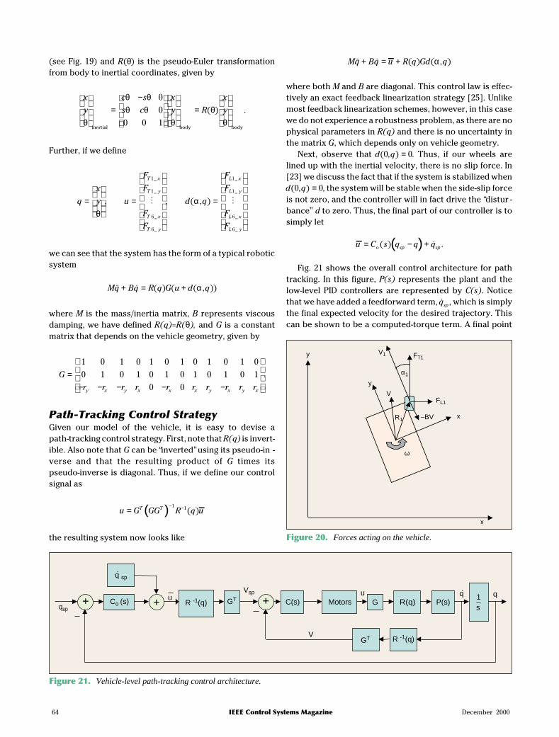
the forces used in our model are shown in Fig. 20. In thesefigures, note especially the angle α i , which represents thedifference between the direction the wheel is pointing andthe direction it is traveling. When this angle is zero, we saythat the vehicle is in kinematic equilibrium. When it is non-zero, the wheel will experience a side-slip force.

In our model, we consider three key forces acting on thevehicle:

• The force FTi is the tangential force due to the motor’storque acting to turn the wheel. This force acts in thedirection the wheel is pointing.

• Acting in a direction to oppose motion is a standardglobal energy dissipation force proportional to the ve-hicle velocity and acting in the opposite direction:

F BVdi i= −

where B is the global energy dissipation coefficient, as-sumed to be the same at each wheel. This is basically aviscous friction force that changes from one surface tothe other, but it also includes the motor losses.

• We also include a lateral slip force FLi acting to restorethe vehicle’s inertial velocity to match that of thewheel. This force acts 90° counterclockwise from thedirection the wheel is pointing and has a magnitudegiven by

( )Fmg

eLis i= − −µ τα

61

where m is the vehicle mass, g is the gravitational con-stant, α i is the angle mismatch between the kinematicvelocity and the wheel velocity, µs is the static coeffi-cient of friction for the surface, and τ is a parameterthat depends on the surface [24]. Notice that if α i = 0,

then FLi = 0, so that when the vehicle is in what we call“kinematic motion,” meaning the actual inertial veloc -ity of the vehicle body at each wheel location matchesthe wheel’s velocity, there is no side-slip force.

Using these three forces, we may write the vehicle dy-namics as

( )mx

yF F BV

I R

Ti Li ii

z ii

��

��

= + −

=

=

=

∑ intertial1

6

1

θ ( )6

∑ × + −F F BVTi Li i intertial

where I z is the vehicle’s moment of inertia about the z-axisand Ri is the distance from the vehicle’s geometric center toeach wheel (see Figs. 19 and 20). Next, defining the vehicle’scenter of mass translational motion asV x y T= ( � �) and usingthe basic kinematic relationship V V ri i= + ×ω we can writethe equations of motion as (introducing additional notationto designate the x and y components of the forces acting ateach wheel)

m

m

I

x

y

B

B

z

0 0

0 0

0 0

6 0 0

0 6 0

=−

−��θ 0 0

1 1

−

+

+

Br

x

y

R G

F F

FT x L x

T

��

( )

_ _

θ

θ1 1

6 6

6 6

_ _

_ _

_ _

y L y

T x L x

T y L y

F

F F

F F

+

++

�

body

where

r r rx y= +6 42 2


y

x

Yaw Angle

θ

Figure 18. x, y, and yaw definitions.

Viαi

vi

θiWheel_i

Ri, ri y

Vy vy

Vx

vx θ

x

rx

ry

Body Frame

xInertial Frame

y

Figure 19. Coordinate systems for controller design.

(see Fig. 19) and R(θ) is the pseudo-Euler transformationfrom body to inertial coordinates, given by

x

y

c s

s c

x

y

θ

θ θθ θ

θ

=−

inertial

0

0

0 0 1

=

body body

R

x

y( ) .θθ

Further, if we define

q

x

y u

F

F

F

F

T x

T y

T x

T y

=

=

θ,

_

_

_

_

1

1

6

6

�

=

, ( , )

_

_

_

_

d q

F

F

F

F

L x

L y

L x

L y

α

1

1

6

6

�

we can see that the system has the form of a typical roboticsystem

Mq Bq R q G u d q�� ( ) ( ( , ))+ = + α

where M is the mass/inertia matrix, B represents viscousdamping, we have defined R(q)=R(θ), and G is a constantmatrix that depends on the vehicle geometry, given by

G

r r r r r r r r ry x y x x x y x

=− − − − −

1 0 1 0 1 0 1 0 1 0 1 0

0 1 0 1 0 1 0 1 0 1 0 1

0 0 y xr

.

Path-Tracking Control StrategyGiven our model of the vehicle, it is easy to devise apath-tracking control strategy. First, note that R(q) is invert-ible. Also note that G can be “inverted” using its pseudo-in -verse and that the resulting product of G times itspseudo-inverse is diagonal. Thus, if we define our controlsignal as

( )u G GG R q uT T=− −1 1( )

the resulting system now looks like

Mq Bq u R q Gd q�� ( ) ( , )+ = + α

where both M and B are diagonal. This control law is effec-tively an exact feedback linearization strategy [25]. Unlikemost feedback linearization schemes, however, in this casewe do not experience a robustness problem, as there are nophysical parameters in R(q) and there is no uncertainty inthe matrix G, which depends only on vehicle geometry.

Next, observe that d q( , )0 0= . Thus, if our wheels arelined up with the inertial velocity, there is no slip force. In[23] we discuss the fact that if the system is stabilized whend q( , )0 0= , the system will be stable when the side-slip forceis not zero, and the controller will in fact drive the “distur -bance” d to zero. Thus, the final part of our controller is tosimply let

( )u C s q q qo sp sp= − +( ) � .

Fig. 21 shows the overall control architecture for pathtracking. In this figure, P(s) represents the plant and thelow-level PID controllers are represented by C(s). Noticethat we have added a feedforward term, �qsp , which is simplythe final expected velocity for the desired trajectory. Thiscan be shown to be a computed-torque term. A final point


V1 FT1

α1

y

VFL1

–BVR1 x

ω

x

y

Figure 20. Forces acting on the vehicle.

+ + +qsp

q sp.

C so ( ) uR q-1( ) GT C s( ) Motors

Vsp uG R q( )

VGT R q-1( )

P s( )q.

1_s

q

Figure 21. Vehicle-level path-tracking control architecture.

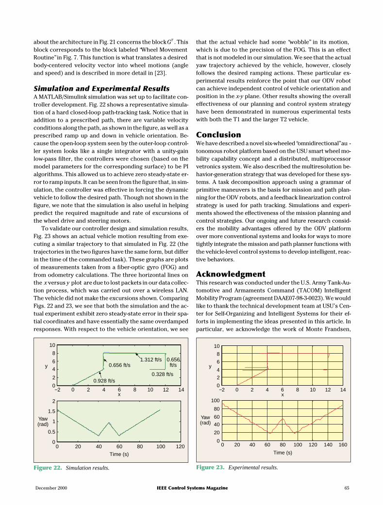
about the architecture in Fig. 21 concerns the blockGT . Thisblock corresponds to the block labeled “Wheel MovementRoutine” in Fig. 7. This function is what translates a desiredbody-centered velocity vector into wheel motions (angleand speed) and is described in more detail in [23].

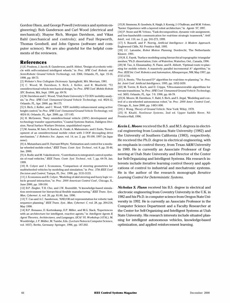
Simulation and Experimental ResultsA MATLAB/Simulink simulation was set up to facilitate con-troller development. Fig. 22 shows a representative simula-tion of a hard closed-loop path-tracking task. Notice that inaddition to a prescribed path, there are variable velocityconditions along the path, as shown in the figure, as well as aprescribed ramp up and down in vehicle orientation. Be-cause the open-loop system seen by the outer-loop control-ler system looks like a single integrator with a unity-gainlow-pass filter, the controllers were chosen (based on themodel parameters for the corresponding surface) to be PIalgorithms. This allowed us to achieve zero steady-state er-ror to ramp inputs. It can be seen from the figure that, in sim-ulation, the controller was effective in forcing the dynamicvehicle to follow the desired path. Though not shown in thefigure, we note that the simulation is also useful in helpingpredict the required magnitude and rate of excursions ofthe wheel drive and steering motors.

To validate our controller design and simulation results,Fig. 23 shows an actual vehicle motion resulting from exe-cuting a similar trajectory to that simulated in Fig. 22 (thetrajectories in the two figures have the same form, but differin the time of the commanded task). These graphs are plotsof measurements taken from a fiber-optic gyro (FOG) andfrom odometry calculations. The three horizontal lines onthe x versus y plot are due to lost packets in our data collec-tion process, which was carried out over a wireless LAN.The vehicle did not make the excursions shown. ComparingFigs. 22 and 23, we see that both the simulation and the ac-tual experiment exhibit zero steady-state error in their spa-tial coordinates and have essentially the same overdampedresponses. With respect to the vehicle orientation, we see

that the actual vehicle had some “wobble” in its motion,which is due to the precision of the FOG. This is an effectthat is not modeled in our simulation. We see that the actualyaw trajectory achieved by the vehicle, however, closelyfollows the desired ramping actions. These particular ex-perimental results reinforce the point that our ODV robotcan achieve independent control of vehicle orientation andposition in the x-y plane. Other results showing the overalleffectiveness of our planning and control system strategyhave been demonstrated in numerous experimental testswith both the T1 and the larger T2 vehicle.

ConclusionWe have described a novel six-wheeled “omnidirectional” au -tonomous robot platform based on the USU smart wheel mo-bility capability concept and a distributed, multiprocessorvetronics system. We also described the multiresolution be-havior-generation strategy that was developed for these sys-tems. A task decomposition approach using a grammar ofprimitive maneuvers is the basis for mission and path plan-ning for the ODV robots, and a feedback linearization controlstrategy is used for path tracking. Simulations and experi-ments showed the effectiveness of the mission planning andcontrol strategies. Our ongoing and future research consid-ers the mobility advantages offered by the ODV platformover more conventional systems and looks for ways to moretightly integrate the mission and path planner functions withthe vehicle-level control systems to develop intelligent, reac-tive behaviors.

AcknowledgmentThis research was conducted under the U.S. Army Tank-Au-tomotive and Armaments Command (TACOM) IntelligentMobility Program (agreement DAAE07-98-3-0023). We wouldlike to thank the technical development team at USU’s Cen-ter for Self-Organizing and Intelligent Systems for their ef-forts in implementing the ideas presented in this article. Inparticular, we acknowledge the work of Monte Frandsen,


−2 0 2 4 6 8 10 12 140

2

4

6

8

10

0.928 ft/s

0.656 ft/s1.312 ft/s

0.328 ft/s

0.656ft/s

0 20 40 60 80 100 1200

0.5

1

1.5

2

Time (s)

y

x

Yaw(rad)

Figure 22. Simulation results.

0

2

4

6

8

10

y

−2 0 2 4 6 8 10 12 14x

0 20 40 60 80 100 120 140 1600

20

40

60

80

100

Yaw(rad)

Time (s)

Figure 23. Experimental results.

Gordon Olsen, and George Powell (vetronics and system en-gineering); Bob Gunderson and Carl Wood (electrical andmechanical); Shayne Rich, Morgan Davidson, and VikasBahl (mechanical and controls); and Paul Hepworth,Thomas Goodsell, and John Ogness (software and com-puter science). We are also grateful for the helpful com-ments of the reviewers.

References[1] E. Poulson, J. Jacob, B. Gunderson, and B. Abbot, “Design of a robotic vehi -cle with self-contained intelligent wheels,” in Proc. SPIE Conf. Robotic andSemi-Robotic Ground Vehicle Technology, vol. 3366, Orlando, FL, Apr. 15-16,1998, pp. 68-73.[2] Webster’s New Collegiate Dictionary. Springfield, MA: Merriam, 1981.[3] C. Wood, M. Davidson, S. Rich, J. Keller, and R. Maxfield, “T2omnidirectional vehicle mechanical design,” in Proc. SPIE Conf. Mobile RobotsXIV, Boston, MA, Sept. 1999, pp. 69-76.[4] M. Davidson and C. Wood, “Utah State University’s T2 ODV mobility analy -sis,” in Proc. SPIE Conf. Unmanned Ground Vehicle Technology, vol. 4024-12,Orlando, FL, Apr. 2000, pp. 96-175.[5] S. Rich, J. Keller, and C. Wood, “ODV mobility enhancement using activeheight control,” in Proc. SPIE Conf. Unmanned Ground Vehicle Technology, vol.4024-16, Orlando, FL, Apr. 2000, pp. 137-145.[6] H. McGowen, “Navy omnidirectional vehicle (ODV) development andtechnology transfer opportunities,” Coastal Systems Station, Dahlgren Divi -sion, Naval Surface Warfare Division, unpublished report.[7] M. Asama, M. Sato, H. Kaetsu, K. Ozaki, A. Matsumoto, and I. Endo, “Devel -opment of an omnidirectional mobile robot with 3 DOF decoupling drivemechanism,” J. Robotics Soc. Japan, vol. 14, no. 2, pp. 95-100, 1997 (in Japa-nese).[8] A. Mutambara and H. Durrant-Whyte, “Estimation and control for a modu-lar wheeled mobile robot,” IEEE Trans. Contr. Syst. Technol., vol. 8, pp. 35-46,Jan. 2000.[9] A. Rodic and M. Vukobratovic, “Contribution to integrated control synthe-sis of road vehicles,” IEEE Trans. Contr. Syst. Technol., vol. 7, pp. 64-78, Jan.1999.[10] R. Colyer and J. Economou, “Comparison of steering geometries formultiwheeled vehicles by modeling and simulation,” in Proc. 37th IEEE Conf.Decision and Control, Tampa, FL, Dec. 1998, pp. 3131-3133.[11] J. Economou and R. Colyer, “Modeling of skid steering and fuzzy logic ve -hicle ground interaction,” in Proc. 2000 American Control Conf., Chicago, IL,June 2000, pp. 100-104.[12] B.P. Ziegler, T.H. Cho, and J.W. Rozenblit, “A knowledge-based simula -tion environment for hierarchical flexible manufacturing,” IEEE Trans. Syst.,Man, Cybernet. A, vol. 26, pp. 81-90, Jan. 1996.[13] T. Cao and A.C. Sanderson, “AND/OR net representation for robotic tasksequence planning,” IEEE Trans. Syst., Man, Cybernet. C, vol. 28, pp. 204-218,May 1998.[14] R.P. Bonasso, D. Kortenkamp, D.P. Miller, and M.G. Slack, “Experienceswith an architecture for intelligent, reactive agents,” in Intelligent Agents II,Agent Theories, Architectures, and Languages, IJCAI ‘95, Workshop (ATAL), M.Wooldridge, J. P. Müller, M. Tambe, Eds. (Lecture Notes in Computer Science,vol. 1037). Berlin, Germany: Springer, 1996, pp. 187-202.

[15] R. Simmons, R. Goodwin, K. Haigh, S. Koenig, J. O’Sullivan, and M.M. Veloso,“Xavier: Experience with a layered robot architecture,” in Agents ‘97, 1997.[16] P. Stone and M. Veloso, “Task decomposition, dynamic role assignment,and low-bandwidth communication for real-time strategic teamwork,” Artif.Intell., vol. 110, no. 2, pp. 241-273, 1999.[17] S. Russell, and P. Norvig, Artificial Intelligence: A Modern Approach.Englewood Cliffs, NJ: Prentice Hall, 1995.[18] J.C. Latombe, Robot Motion Planning. Dordrecht, The Netherlands:Kluwer, 1991.[19] R. E. Fayek, “Surface modeling using hierarchical topographic triangularmeshes,” Ph.D. dissertation, Univ. of Waterloo, Waterloo, Ont., Canada, 1996.[20] M. Tao, A. Elssamadisy, N. Flann, and B. Abbott, “Optimal route re-plan -ning for mobile robots: A massively parallel incremental A* algorithm,” inProc. IEEE Int. Conf. Robotics and Automation, Albuquerque, NM, May 1997, pp.2727-2735.[21] A. Stentz, “The focused D* algorithm for real-time re-planning.” in Proc.Int. Joint Conf. Artificial Intelligence, 1995, pp. 1652-1659.[22] M. Torrie, R. Koch, and D. Cripps, “Ultra-maneuverable algorithms forterrain transitions,” in Proc. SPIE Conf. Unmanned Ground Vehicle Technology,vol. 3693, Orlando, FL, Apr. 7-9, 1998, pp. 66-78.[23] K. Moore, M. Davidson, V. Bahl, S. Rich, and S. Jirgal, “Modeling and con -trol of a six-wheeled autonomous robot,” in Proc. 2000 Amer. Control Conf.,Chicago, IL, June 2000, pp. 1483-1490.[24] J. Wong, Theory of Ground Vehicle. New York: Wiley, 1978.[25] H. Khalil, Nonlinear Systems, 2nd ed. Upper Saddle River, NJ:Prentice-Hall, 1996.

Kevin L. Moore received the B.S. and M.S. degrees in electri-cal engineering from Louisiana State University (1982) andthe University of Southern California (1983), respectively.He received the Ph.D. degree in electrical engineering, withan emphasis in control theory, from Texas A&M Universityin 1989. He is currently an Associate Professor of Engi-neering at Utah State University and Director of the Centerfor Self-Organizing and Intelligent Systems. His research in-terests include iterative learning control theory and appli-cations of control to industrial and mechatronic systems.He is the author of the research monograph IterativeLearning Control for Deterministic Systems.

Nicholas S. Flann received his B.S. degree in electrical andelectronic engineering from Coventry University in the U.K. in1982 and his Ph.D. in computer science from Oregon State Uni-versity in 1992. He is currently an Associate Professor in theComputer Science Department and a Faculty Researcher atthe Center for Self-Organizing and Intelligent Systems at UtahState University. His research interests include situated plan-ning for intelligent autonomous vehicles, knowledge-basedoptimization, and applied reinforcement learning.


Documents

A six-wheeled omnidirectional autonomous mobile robot