Hacettepe Journal of Mathematics and StatisticsVolume 46 (3) (2017), 555 � 565

A single pairwise model for classi�cation usingonline learning with kernels

Engin Tas ∗†

Abstract

Any binary or multi-class classi�cation problem can be transformedinto a pairwise prediction problem. This expands the data and bringsan advantage of learning from a richer set of examples, in the expenseof increasing costs when the data is in higher dimensions. Therefore,this study proposes to adopt an online support vector machine to workwith pairs of examples. This modi�ed algorithm is suitable for largedata sets due to its online nature and it can also handle the sparsitystructure existing in the data. Performances of the pairwise setting andthe direct setting are compared in two problems from di�erent domains.Results indicate that the pairwise setting outperforms the direct settingsigni�cantly. Furthermore, a general framework is designed to use thispairwise approach in a multi-class classi�cation task. Result indicatethat this single pairwise model achieved competitive classi�cation rateseven in large-scaled datasets with higher dimensionality.

Keywords: online learning, pairwise learning, support vector machines, kernel

methods, multi-class classi�cation.

2000 AMS Classi�cation: 68W27, 62H30, 68T05, 68Q32

Received : 23.06.2016 Accepted : 02.08.2016 Doi : 10.15672/HJMS.2017.416

∗Department of Statistics, Faculty of Science and Literature, Afyon Kocatepe UniversityEmail: engintas@aku.edu.tr†Corresponding Author.

556

1. Introduction

In multi-class classi�cation, we have a set of examples each belongs to one of theM di�erent classes. The task is to learn a classi�cation function which, given a newexample, will predict the class to which the new observation belongs. Learning processstarts by introducing a loss function which measures the error between the predictionand the actual class of the new example. An empirical risk function is then de�ned overa training data to estimate this loss accordingly. For instance, in classi�cation tasks, wetry to minimize the cost we pay for incorrectly assigning the examples to the wrong class.

There are two basic schemes in multi-class classi�cation. The �rst one is one-versus-all (OVA) which we �nd M di�erent binary classi�cation functions, each one try todiscriminate the examples in a single class from the examples in all remaining classes.For the ith classi�er, we let the positive examples be all the observations in class i, andlet the negative examples be all the observations not in class i. The second scheme, all-versus-all (AVA), builds M(M − 1)/2 binary classi�ers, one classi�er for separating eachpair of classes i and j. In both schemes, a new example is attained to the class whichhas the highest classi�er score. Although, there exist so many studies proposing morecomplicated methods for multi-class classi�cation, a recent study [27] showed that theOVA scheme is extremely powerful, using well-tuned binary classi�ers such as supportvector machines (SVMs), producing results that are often at least as accurate as othermethods. In these approaches, the main problem lies in the fact that one has to �ndan e�ective way of combining di�erent binary classi�er functions in a single multi-classclassi�cation model.

The critical point in multi-class classi�cation is to have a powerful binary classi�errather than a search for much more complex models. The central idea of SVM is toconstruct an optimal separating hyperplane over linearly separable data [5]. It can alsolearn a large margin hyperplane over linearly inseparable data by using kernels and softmargin formulations. SVMs also impose a form of regularization by controlling the ca-pacity of the classi�er function in order to avoid over-�tting or under-�tting problem.This provides a key support in building powerful binary classi�ers. However, SVM isoriginally designed for binary classi�cation and there are two principal approaches forextending SVM to the multi-class scenario. One approach is to generalize the binaryalgorithm to multi-class [25, 15], another approach is to decompose the multi-class prob-lem into a series of binary problems. Pairwise classi�cation is an alternative techniquefor solving multi-class problems by considering pairwise comparisons obtained from eachof the two-class problems [10]. A test observation is assigned to the class that wins themost pairwise comparisons.

In this paper, we recast the multi-class classi�cation problem in a pairwise setting.Let us denote a pair formed by two examples from the same class as a positive pairand a pair formed by two examples from di�erent classes as a negative pair. Then, weconstruct a single pairwise SVM model for classifying pairs This pairwise SVM modelis able to identify a given pair, whether it is a positive pair or not. However, in apairwise setting n examples correspond to n2 pairwise examples and training a supportvector machine with such amount of data introduces serious computational costs in mostcases with large scaled data. SVMs, in the batch setting, requires the evaluation of theobjective function at each step and this involves basically the summation of a prede�nedloss over a set of data to be trained. Gradient-based methods must compute this sumfor each evaluation of the objective, respectively its gradient whereas standard numericaloptimization techniques such as variation of Newton's method, and the conjugate gradientalgorithm needs the second-order information of the objective function. As available data

557

sets grow ever larger, such classical second-order methods are impractical in almost alluseful cases.

Online gradient-based methods such as Perceptron [19, 16] and its variants [1, 9, 14,11], by contrast, have a major advantage in large and redundant data sets. In fact,simple online gradient descent [6, 26, 21] outperforms sophisticated second-order batchmethods in general since the computational requirements of online methods are extremelyreduced by the fact that they only process examples one by one or small sub-samples ofthe training data. Therefore, this work depends on two basic ideas related to the problemsetting and the choice of a proper method. First, we know that any binary or multi-classclassi�cation problem can be converted into a pairwise classi�cation problem. This bringsan advantage of learning from a larger data set of pairs. Secondly, traditional learningalgorithms become ine�cient in this setting and in some cases impossible to apply (e.g.batch methods), we propose to modify our single pairwise SVM algorithm to work withpairs of examples in an online manner. This brings an advantage of processing pairsone by one and overcomes the di�culties arising from large scaled data with higherdimensions.

2. General Framework

We have a set of examples X = (x1, x2, ..., xm),∀xi ∈ Rn. One can think of anycombination of two examples as a pair p = (xi, xj) ∈ P ⊆ X2 and denote a sequenceT = {(p, yp) : p ∈ P} be a training sample drawn according to a probability distributionover a sample space Z = P×{+1,−1}. An example from T is a triple consisting of a pairof an n-dimensional column vector of real-valued features and a corresponding label ypindicating whether an interaction exists between these two pairs of examples. The task isto learn a suitable function f : P→ {+1,−1} from the training sample. We consider thelinear case where the decision function represented as f(p) = 〈w,Φ(p)〉, where w ∈ Rn isa vector of parameters that needs to be estimated based on training sample T .

An optimal decision function (optimal hyperplane with the biggest margin) is foundby minimizing the following objective function in the feature space [20]:

(2.1) minw‖w‖2 + C

n∑i=1

ξi with

{∀i yiy(pi) ≥ 1− ξi∀i ξi ≥ 0

The slack variables ξ = ξ1, ξ2, . . . , ξn allow for some pairs to be on the wrong side of themargin. For very large values of the regularization parameter C, we have a high penaltyfor nonseparable examples and we may store many support vectors. Smaller values of Csoftens the e�ect of this penalty and produce better results on noisy problems but, wemay have the risk of under�tting.

Maximizing the dual of this convex optimization problem is a simpler convex qua-dratic programming problem than the primal 2.1. The coe�cients αi of the SVM kernelexpansion are found by de�ning the dual objective function.

(2.2) W (α) =∑i

αiyi −1

2

∑i,j

αiαjK(pi, pj)

and solving the SVM Quadratic Programming (QP) problem:

(2.3) maxα

W (α) with

∑i αi = 0

Ai ≤ αi ≤ BiAi = min(0, Cyi)

Bi = max(0, Cyi).

558

Since we have a large number of growing pairs even in moderate size data sets, weneed an e�ective SVM solver to handle these large data sets with large dimensions. A fastkernel classi�er with online and active learning LASVM ‡ [4] is used to overcome thesetypes of di�culties. Due to its online nature, it has several advantages in the pairwisesetting. LASVM deals with complexity problems by processing examples one by one andkeeping the most informative support vectors in its expansion. This reduces the amountof calculations signi�cantly. Another advantage of LASVM is its compatibility for sparsedata sets since the main problem in working with large dimensions, most of the data setshave a critical sparsity structure. LASVM overcomes this problem using convenient fastsparse vector products. This brings the bene�ts of learning from a richer data set formedby the combination of examples and by processing pairs of examples online. LASVMintroduces a support vector removal step which means that the vectors collected in thecurrent kernel expansion can be removed during the online process. It is also related tothe sequential minimal optimization (SMO) [18] algorithm and converges to the solutionof the SVM quadratic programming problem.

LASVM itself is not suitable for a pairwise setting. Because, in this form, you have touse its kernel cache to keep the kernel values between pairs and this brings quite expensivecosts. This makes the algorithm unscalable to large data sets. It's also meaningless tokeep kernel values between pairs, because once you have the kernel values between theseexamples than you need three operations to calculate the kernel value between any pair.Therefore, in this study, there are several modi�cations made at the implementationlevel in order to adapt LASVM to work in the pairwise setting. We name the resultingalgorithm as pw-LASVM. The �rst main contribution of this paper is the following basemodi�cations to LASVM in order to build pw-LASVM.

• We de�ne the set P and S to keep the indices of the support pairs and the in-dices of the corresponding examples of the pairs respectively. When pw-LASVMinserts one pair to its current kernel expansion (process), we insert the index ofthe pair into the set P , and simultaneously add the corresponding indices of thetwo examples into the set S. We use the set P just to keep the indices of thepairs, it does not have a kernel cache since the kernel values are calculated forthe examples as we mentioned before. On the other hand, the set S has a kernelcache which keeps the kernel values between examples.

• All the procedures for processing an example are modi�ed to process a pair ofexamples. This includes the calculation of the gradient of a pair, identi�cationof the τ -violating quadruple (formed by two pairs) with the maximal gradientand the direction searches.

• Reprocess removes some pairs from P . This corresponds to removing two ex-amples of the related pair from the set S. Finally all the quantities like thebias term b and the gradient δ of the most τ -violating quadruple in the P arecomputed.

LASVM is an online kernel classi�er introducing a support vector removal step whichmeans that the vectors collected in the current kernel expansion can be removed duringthe online process. It is also related to the sequential minimal optimization (SMO) [18]algorithm and converges to the solution of the SVM quadratic programming problem.As LASVM is adapted to work with pairs of examples, it is named as pw-LASVM. It�rst inserts at least one pair into its current kernel expansion (process) and then searchesfor redundant support pairs that are already existed in the current kernel expansion(reprocess). In the online setting, this can be used to process a new pair at time t. Now,the pairs in the current kernel expansion with coe�cient αi 6= 0 are called support pairs

‡http://leon.bottou.org/projects/lasvm

559

and the indices in the set S of potential support pairs correspond to the indices of pairs.The coe�cient αi are assumed to be null if i /∈ S.

In a pairwise setting, the structure of pw-LASVM deserves much more attention, sincethe process and reprocess steps nicely retain more informative pairs and bail out the pairsthat are not needed in the current kernel expansion. This is most useful in the pairwisesetting where the pairs grow quadratically with the size of the data set.

2.1. Pairwise setting. Let's start with two introductory examples to explain the pair-wise setting of the problem. First, assume a network formed by a set of proteins whereone can observe several interactions between these proteins according to a particular bi-ological function. A link is created between two proteins whenever an interaction occurs.Basically, the data we have from this event is the features of these proteins and a positivelabel indicating the interaction. This data can basically be structured in two ways:

- In the direct setting, two proteins are regarded as one example by combiningtheir features and assigning a positive class membership. A sample of examplesfrom negative class can also be generated in a similar way considering non-interacting proteins. If a new protein joins into this network, in order to predictnew links between the new protein and existing ones, features of the new proteinand the features of any existing protein in the network are combined as if a newexample and compared with the examples which were previously formed and alabel is assigned indicating the relation (interacting or non-interacting).

- In the indirect (pairwise) setting, we can think of two interacting proteins as apositive pair and two non-interacting proteins as a negative pair. There is nofeature conjunction in this setup. Comparisons are made in a pairwise mannerwhere all combinational relations considered between the members of the twopairs. In the �rst setup, the problem is de�ned as a standard binary classi�cationtask whereas in the second setting we have a link prediction problem betweenpairs of proteins. Consequently, the structure of the data we have also dependson the problem setup. Finally, this approach can also be applied in binaryclassi�cation problems.

In order to learn a mapping from pairs, we need an additional type of structure forrepresenting a pair in a joint feature space. [2] uni�ed user ratings and item featuresin a common learning architecture and gave good examples of designing suitable kernelsfor di�erent pairs of examples and also illustrated several ways of combining kernels intoa single kernel. They used tensor products to simply join distinct feature maps. [17]proposed a kernel method for using combinations of features across example pairs inlearning pairwise classi�ers. In this context, [3] proposed the tensor product pairwisekernel (TPPK) that converts a kernel between single proteins into a kernel betweenpairs of proteins, and illustrated the kernel's e�ectiveness in conjunction with a supportvector machine classi�er. [23] proposed the metric learning pairwise kernel (MLPK) forthe reconstruction of biological networks. [13] proposed a special case of this generalframework where they used Cartesian kernel to speed up the online training processsince, Cartesian kernel has a much sparser structure than TPPK and MLPK. They alsoprovide generalization bounds for the two pairwise kernels based on eigenvalue analysisof the kernel matrices.

In this paper, we used TPPK in the conjunction with an element-wise kernel betweenexamples. TPPK between the pairs p1 = (x1, x2) and p2 = (x3, x4) is given as

(2.4) KTPPK((x1, x2), (x3, x4)) = K(x1, x3)K(x2, x4) +K(x1, x4)K(x2, x3).

With an appropriate choice for element-wise kernel, such as the Gaussian RBF kernel,the kernel TPPK generates a class H of universally approximating functions for learning

560

any type of relation between pairs. We had also examined the performance of MLPK inall experiments and didn't �nd any statistically signi�cant di�erences from TPPK.

3. Experiments

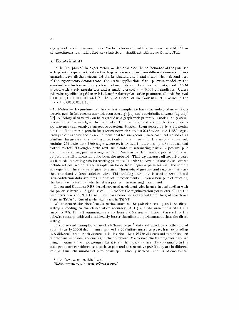
In the �rst part of the experiments, we demonstrated the performance of the pairwisesetting with respect to the direct setting in two examples from di�erent domains. Theseexamples have distinct characteristics in dimensionality and sample size. Second partof the experiments demonstrates the useful application of the pairwise model on thestandard multi-class or binary classi�cation problems. In all experiments, pw-LASVMis used with a soft margin loss and a small tolerance τ = 0.001 on gradients. Unlessotherwise speci�ed, a grid-search is done for the regularization parameter C in the interval[0.001, 0.1, 1, 10, 100, 100] and for the γ parameter of the Gaussian RBF kernel in theinterval [0.001, 0.01, 1, 10].

3.1. Pairwise Experiments. In the �rst example, we have two biological networks, aprotein-protein interaction network (von-Mering) [24] and a metabolic network (ligand)�

[22]. A biological network can be regarded as a graph with proteins as nodes and protein-protein relations as edges. In each network, an edge indicates that the two proteinsare enzymes that catalyze successive reactions between them according to a particularfunction. The protein-protein interaction network contains 2617 nodes and 11855 edges.Each protein is described by a 76-dimensional feature vector, where each feature indicateswhether the protein is related to a particular function or not. The metabolic networkcontains 755 nodes and 7860 edges where each protein is described by a 36-dimensionalfeature vector. Throughout the text, we denote an interacting pair as a positive pairand non-interacting pair as a negative pair. We start with forming a positive pairs setby obtaining all interacting pairs from the network. Then we generate all negative pairsset from the remaining non-interacting proteins. In order to have a balanced data set weinclude all positive pairs and sample randomly from negative pairs set with the samplesize equals to the number of positive pairs. These sets of positive and negative pairs arethen combined to form training pairs. This training pairs data is used to create 3 × 5cross-validation data sets for the �rst set of experiments. Given a new pair of proteins,the task is to determine whether it's a positive (interacting) pair or not.

Linear and Gaussian RBF kernels are used as element-wise kernels in conjunction withthe pairwise kernels. A grid search is done for the regularization parameter C and theparameter γ of the RBF kernel. Best parameter pairs obtained from the grid-search aregiven in Table 1. Kernel cache size is set to 256MB.

We compared the classi�cation performance of the pairwise setting and the directsetting according to the classi�cation accuracy (ACC) and the area under the ROCcurve (AUC). Table 2 summarizes results from 3 × 5 cross validation. We see that thepairwise settings achieved signi�cantly better classi�cation performances than the directsetting.

In the second example, we used 20-Newsgroups ¶ data set which is a collection ofapproximately 20000 documents organized in 20 distinct newsgroups, each correspondingto a di�erent topic. Each document is described by a 25736-dimensional vector formedby frequencies of words occurring in the document. We formed the training pair data setusing documents from two groups related to sports and computers. Two documents in thesame group are considered as a positive pair and as a negative pair if they are in di�erentgroups. Since the number of pairs grows quadratically with the number of documents.

�http://www.genome.ad.jp/ligand¶http://qwone.com/∼jason/20Newsgroups/

561

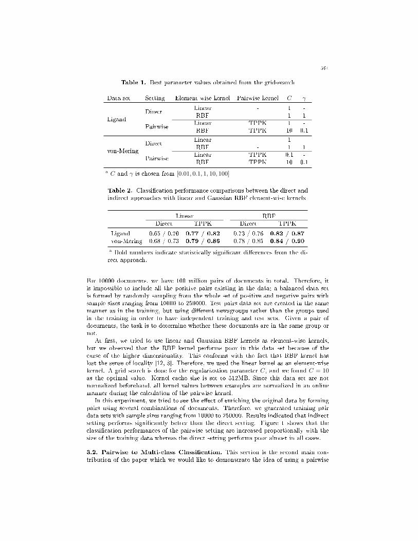
Table 1. Best parameter values obtained from the grid-search

Data set Setting Element-wise kernel Pairwise kernel C γ

LigandDirect

Linear - 1 -RBF - 1 1

PairwiseLinear TPPK 1 -RBF TPPK 10 0.1

von-MeringDirect

Linear - 1 -RBF - 1 1

PairwiseLinear TPPK 0.1 -RBF TPPK 10 0.1

a C and γ is chosen from [0.01, 0.1, 1, 10, 100]

Table 2. Classi�cation performance comparisons between the direct andindirect approaches with linear and Gaussian RBF element-wise kernels

Linear RBFDirect TPPK Direct TPPK

Ligand 0.65 / 0.70 0.77 / 0.82 0.73 / 0.76 0.82 / 0.87von-Mering 0.68 / 0.73 0.79 / 0.86 0.78 / 0.85 0.84 / 0.90

a Bold numbers indicate statistically signi�cant di�erences from the di-rect approach.

For 10000 documents, we have 100 million pairs of documents in total. Therefore, itis impossible to include all the positive pairs existing in the data; a balanced data setis formed by randomly sampling from the whole set of positive and negative pairs withsample sizes ranging from 10000 to 250000. Test pairs data set are created in the samemanner as in the training, but using di�erent newsgroups rather than the groups usedin the training in order to have independent training and test sets. Given a pair ofdocuments, the task is to determine whether these documents are in the same group ornot.

At �rst, we tried to use linear and Gaussian RBF kernels as element-wise kernels,but we observed that the RBF kernel performs poor in this data set because of thecurse of the higher dimensionality. This conforms with the fact that RBF kernel haslost the sense of locality [12, 8]. Therefore, we used the linear kernel as an element-wisekernel. A grid search is done for the regularization parameter C, and we found C = 10as the optimal value. Kernel cache size is set to 512MB. Since this data set are notnormalized beforehand, all kernel values between examples are normalized in an onlinemanner during the calculation of the pairwise kernel.

In this experiment, we tried to see the e�ect of enriching the original data by formingpairs using several combinations of documents. Therefore, we generated training pairdata sets with sample sizes ranging from 10000 to 250000. Results indicated that indirectsetting performs signi�cantly better than the direct setting. Figure 1 shows that theclassi�cation performances of the pairwise setting are increased proportionally with thesize of the training data whereas the direct setting performs poor almost in all cases.

3.2. Pairwise to Multi-class Classi�cation. This section is the second main con-tribution of the paper which we would like to demonstrate the idea of using a pairwise

562

Figure 1. Classi�cation performances in 20-Newsgroups data setusing criteria a)ACC b)AUC

SVM model in a multi-class classi�cation task. Let us start with an introductory examplewhich is a simple character recognition task. First, assume that each example in the dataset represents a character written in a speci�c font. We coded these characters with aletter and a number (A1, A2, B1, B3, C1, C2, etc.) in 2. We used A1 and A2 to denotethe binary images of handwritten letter "A" which are written in di�erent fonts. Thetask is to recognize these characters and assign the correct label (A,B,C, etc.).

We can think of the whole process in two stages such as the training and the testing.The �rst step is to preprocess the data in order to make it convenient for pairwiselearning. Therefore, the data is divided into three sets such as train, validation andtest. Then, pairwise train data is formed by taking all pairwise combinations (if possible,otherwise we randomly sample from all pairwise combinations) in the train set and apairwise validation data is formed similarly by taking all possible pairwise combinationsin the validation set. These pairwise data sets are formed by positive and negative pairsof examples, where we assign a positive label if it includes two examples from the sameclass and a negative label if it includes examples form di�erent classes. An online pairwiseSVM model is trained on pairwise train data. Pairwise classi�cation performance of thetrained SVMmodel is evaluated on the pairwise validation data and the hyper-parametersof the model is tuned. Once an ideal model is built, we proceed to the testing stage.

In the testing stage, consider a test example which we have never seen before, we coupleit with a speci�c number (ex. 100) of train examples. Proceeding in this way, by couplingtest examples with a speci�ed number of train examples (with known labels), we form thepairwise test data. This pairwise test data is given as an input to the built pairwise SVMmodel and the pairwise predictions obtained. Once we have these predictions, we havethe votes of the speci�ed number of train examples for the corresponding test example.This provides us with the information whether the test example is coming from the sameclass of the corresponding training example or not. In other words, every train examplein a pair gives a vote to the test example whether it's coming from the same class or not.Finally, we simply use the majority vote to assign the test example to the winning class.The whole process is illustrated in Figure 2.

For the �nal experiments, 20-Newsgroups and MNIST ‖ datasets are used for multi-class classi�cation. 20-Newsgroups datasets is used again in the �nal experiments inorder to demonstrate the scalability of the pw-LASVM and the above approach. Up to

‖http://yann.lecun.com/exdb/mnist

563

Figure 2. Schematic illustration of multi-class classi�cation using pw-LASVM

Table 3. Pairwise and �nal classi�cation accuracies of best models trained accordingto the given process in �gure 2

Nr. oftraining pairs

Nr. ofvoters

Pairwiseaccuracy

Finalaccuracy

Data

set 20-Newsgroups 250000 200 90.09 83.00

MNIST 100000 100 95.89 94.00

now, multi-class classi�cation experiments are limited to small-scaled datasets both insample size and dimensionality. MNIST dataset is chosen in order to see the performanceof the new approach in a problem with low dimensionality.

In 20-Newsgroups experiments, linear kernel is used as element-wise kernel, pw-LASVMis initialized with a regularization parameter C = 10. Kernel cache size is set to 1024MB.Since this data set are not normalized beforehand, all kernel values between examplesare normalized in an online manner during the calculation of the pairwise kernel. In

564

MNIST experiments, Gaussian RBF kernel is used with γ = 0.01 as element-wise kernel,C = 1000 is set for the regularization parameter.

Results of the �nal experiments are summarized in Table 3. Although, these arenot the best results when comparing with the existing methods in the literature, it'snoteworthy that pw-LASVM achieved these classi�cation performances using a singlepairwise model which is totally di�erent from general approaches such as "one-against-all" and "one-against-one".

4. Conclusion

pw-LASVM is developed by e�ectively modifying the LASVM algorithm as to workwith pairs of examples. Performance of the pw-LASVM is demonstrated in two types ofrelational networks. Results demonstrated that, the pairwise approach achieved a betterperformance than the direct approach. A general framework is built in order to solvemulti-class classi�cation problems with pw-LASVM. Final experiments indicate that theproposed approach is scalable to large datasets with higher dimensionality.

pw-LASVM can be used in binary, multi-class classi�cation problems in domains suchas statistics, �nance, information retrieval,collaborative �ltering and social network anal-ysis where the data is very large with higher dimensionality. On the other hand, in do-mains like bioinformatics, genetics and biostatistics, since the cost of obtaining a sampleis quite high, we have data sets with small sample sizes in classi�cation or link predic-tion problems. This makes the model building process much harder because there isnot enough data to validate or even test the model performance. In these cases, thisapproach can also be applied since one can extend this data by transforming the classi-�cation problem into a pairwise setting, and use pw-LASVM as an e�ective online SVMsolver which can work with pairs of examples using suitable pairwise kernels.

References

[1] Anlauf, J. and Biehl, M. (2007). The adatron: an adaptive perceptron algorithm. EPL(Europhysics Letters), 10(7), 687.

[2] Basilico, J. and Hofmann, T. (2004). Unifying collaborative and content-based �ltering. InProceedings of the twenty-�rst international conference on Machine learning, ICML '04,pages 9�, New York, NY, USA, 2004. ACM. ISBN 1-58113-838-5. doi: 10.1145/1015330.1015394. URL http://doi.acm.org/10.1145/1015330.1015394.

[3] Ben-Hur, A. and Noble, W. (2005). Kernel methods for predicting protein-protein interac-tions. Bioinformatics, 21(suppl 1), i38�i46.

[4] Bordes, A., Ertekin, S., Weston, J., and Bottou, L. (2005). Fast kernel classi�ers with onlineand active learning. Journal of Machine Learning Research, 6, 1579�1619.

[5] Boser, B., Guyon, I., and Vapnik, V. (1992). A training algorithm for optimal marginclassi�ers. In Proceedings of the �fth annual workshop on Computational learning theory,pages 144�152. ACM.

[6] Bottou, L. and LeCun, Y. (2004). Large scale online learning. In Thrun, S., Saul, L., andSchölkopf, B., editors, Advances in Neural Information Processing Systems 16. MIT Press,Cambridge, MA. URL http://leon.bottou.org/papers/bottou-lecun-2004.

[7] Dietterich, T. and Bakiri, G. (1995). Solving multiclass learning problems via error-correcting output codes. Journal of Arti�cial Intelligence Research, 2(263), 286.

[8] Francois, D., Wertz, V., and Verleysen, M. (2005). About the locality of kernels in high-dimensional spaces. In Proceedings of ASMDA 2005, International Symposium on AppliedStochastic Models and Data Analysis, pages 238�245. URL http://hdl.handle.net/2078.

1/93830.[9] Freund, Y. and Schapire, R. (1999). Large margin classi�cation using the perceptron algo-

rithm. Machine learning, 37(3), 277�296.

565

[10] Friedman, J. (1996). Another approach to polychotomous classifcation. Technical report,Technical report, Stanford University, Department of Statistics.

[11] Gentile, C. (2002). A new approximate maximal margin classi�cation algorithm. J. Mach.Learn. Res., 2, 213�242. ISSN 1532-4435. URL http://portal.acm.org/citation.cfm?id=

944790.944811.[12] Hastie, T., Tibshirani, R., and Friedman, J. (2009). The Elements of Statistical Learning:

Data Mining, Inference, and Prediction. Springer, 2 edition. ISBN 0387927091. URL http:

//www-stat.stanford.edu/~tibs/ElemStatLearn/.[13] Kashima, H., Oyama, S., Yamanishi, Y., and Tsuda, K. (2009). On Pairwise Kernels: An

E�cient Alternative and Generalization Analysis. In Proceedings of the 13th Paci�c-AsiaConference on Advances in Knowledge Discovery and Data Mining, PAKDD '09, pages1030�1037, Berlin, Heidelberg, 2009. Springer-Verlag. ISBN 978-3-642-01306-5. URL http:

//dx.doi.org/10.1007/978-3-642-01307-2\_110.[14] Li, Y. and Long, P. (2002). The relaxed online maximum margin algorithm. Machine Learn-

ing, 46(1), 361�387.[15] Mayoraz, E. and Alpaydin, E. (1999). Support vector machines for multi-class classi�cation.

Engineering Applications of Bio-Inspired Arti�cial Neural Networks, pages 833�842.[16] Minsky, M. and Seymour, P. (1969). Perceptrons.[17] Oyama, S. and Manning, C. D. (2004). Using feature conjunctions across examples for learn-

ing pairwise classi�ers. In 15th European Conference on Machine Learning (ECML2004).URL http://ilpubs.stanford.edu:8090/767/.

[18] Platt, J. C. (1999). 12 fast training of support vector machines using sequential minimaloptimization.

[19] Rosenblatt, F. (1958). The perceptron: a probabilistic model for information storage andorganization in the brain. Psychological review, 65(6), 386.

[20] Schölkopf, B. and Smola, A. (2001). Learning with kernels: Support vector machines, regu-larization, optimization, and beyond. MIT press.

[21] Shalev-Shwartz, S., Singer, Y., and Srebro, N. (2007). Pegasos: Primal estimated sub-gradient solver for svm. In Proceedings of the 24th international conference on Machinelearning, pages 807�814. ACM.

[22] Vert, J.-P. and Kanehisa, M. (2003). Graph-driven features extraction from microarray datausing di�usion kernels and kernel cca. Advances in Neural Information Processing System,5, 1425�1432.

[23] Vert, J.-P., Qiu, J., and Noble, W. (2007). A new pairwise kernel for biological networkinference with support vector machines. BMC Bioinformatics, 8(Suppl 10), S8.

[24] von Mering, C., Krause, R., Snel, B., Cornell, M., Oliver, S. G., Fields, S., and Bork,P. (2002). Comparative assessment of large-scale data sets of protein�protein interactions.Nature, 417(6887), 399�403.

[25] Weston, J. and Watkins, C. (1999). Support vector machines for multi-class pattern recog-nition. In Proceedings of the seventh European symposium on arti�cial neural networks,volume 4, pages 219�224.

[26] Xu, W. (2011). Towards optimal one pass large scale learning with averaged stochasticgradient descent. arXiv preprint arXiv:1107.2490.

[27] Rifkin, R. and Klautau, A. (2004). In defense of one-vs-all classi�cation. Journal of machinelearning research, volume 5, pages 101�141.

Appendices

The codes developed and the datas used in this paper can be found under the linkhttp://blog.aku.edu.tr/engintas/publications/