A simulation-optimization-based decision support system

for water allocation

14. Workshop Modellierung und Simulation von Ökosystemen

27.10-29.10.2010

Divas Karimanzira

• Goals

• Problem situation

• Structure of the decision support system

• Selected results

• Benefits and applications

• Conclusions

2

3

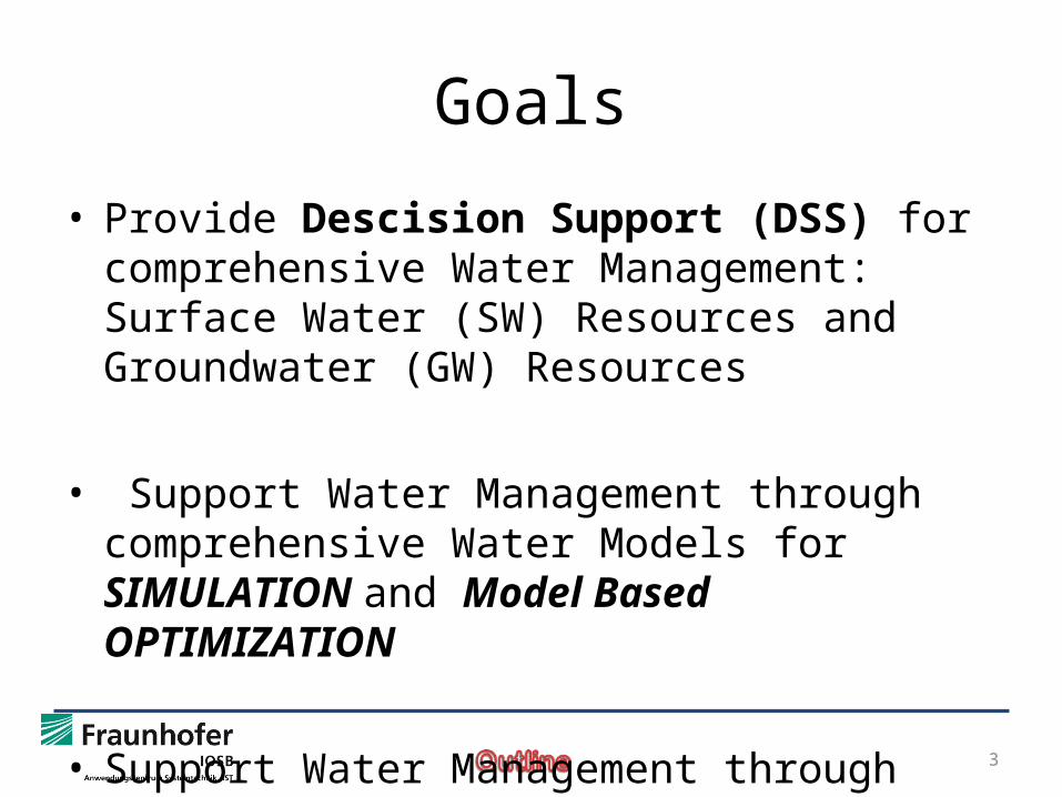
Goals

• Provide Descision Support (DSS) for comprehensive Water Management: Surface Water (SW) Resources and Groundwater (GW) Resources

• Support Water Management through comprehensive Water Models for SIMULATION and Model Based OPTIMIZATION

• Support Water Management through SCENARIOS

4

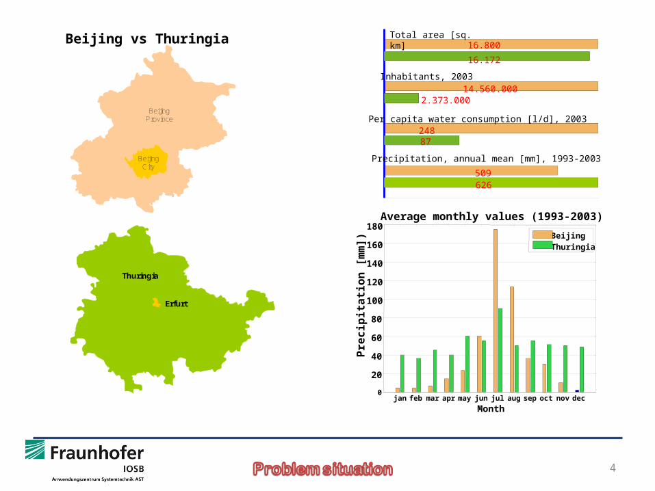
Beijing vs Thuringia

BeijingCity

BeijingProvince

Erfurt

Thuringia

Total area [sq. km]

Inhabitants, 2003

Per capita water consumption [l/d], 2003

Precipitation, annual mean [mm], 1993-2003

509626

24887

16.800

16.172

14.560.0002.373.000

jan feb mar apr may jun jul aug sep oct nov dec0

20

40

60

80

100

120

140

160

180

Pre

cip

itati

on

[m

m])

Month

Average monthly values (1993-2003)

BeijingThuringia

5

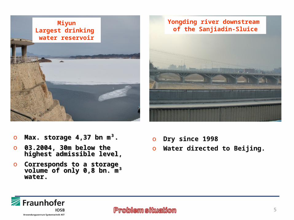
Yongding river downstream of the Sanjiadin-Sluice

MiyunLargest drinking water reservoir

o Dry since 1998o Water directed to Beijing.

o Max. storage 4,37 bn m³. Max. storage 4,37 bn m³. o 03.2004, 30m below the highest 03.2004, 30m below the highest

admissible level, admissible level, o Corresponds to a storage volume of only Corresponds to a storage volume of only

0,8 bn. m³ water.0,8 bn. m³ water.

6

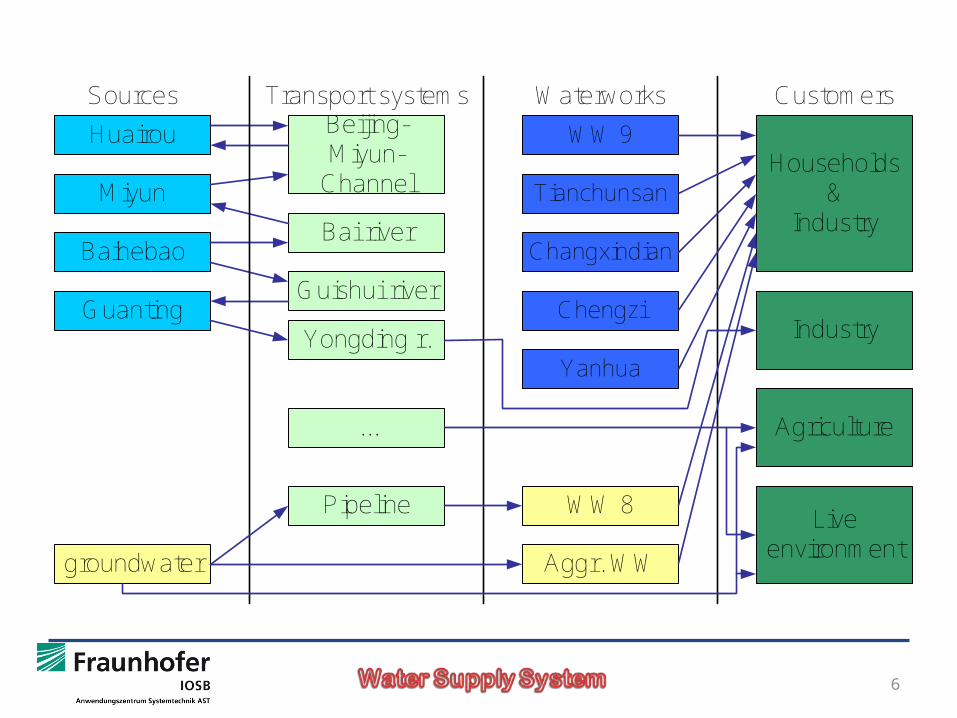
Miyun

Huairou

Baihebao

Guanting

groundwater

SourcesBeijing-Miyun-

Channel

Guishui river

Bai river

Yongding r.

...

Transport systems

WW 9

Tianchunsan

Waterworks

Changxindian

Aggr. WW

WW 8

Customers

Households&

Industry

Industry

Agriculture

Live environment

Pipeline

Chengzi

Yanhua

• Groundwater is the most important source of water for the Beijing region covering 50-70%

• Almost all available groundwater resources are already developed.

• Beijing has suffered from over exploitation of this source. • Surface water supply in the Beijing region depend mainly

on upstream inflows (Chaobai, North Grand Canal, Yongding)

Problems: • excessive withdrawal • lack of regional coordination leads to issues such as

– uncoordinated withdrawals

– and upstream water contamination.

7

8

• Data to identify and describe the physical, social, legal, economic, and institutional factors that affect water resources management.

• Climatic factors such as temperature, wind, solar radiation, and rainfall

• Water quantity and quality demands over time and space

• Land-use and geomorphic information (e.g., slopes, drainage density, geology, Soils, land covers, channel cross-sections, and groundwater depths);

• Hydrologic data that include flows, water levels, depths, and velocities;

• Pollutant loads from point sources (e.g., cities, industries, and wastewater

• Treatment plants that discharge their wastes into surface waters and

• Pollutant loads from nonpoint sources that enter surface waters along an entire stretch of the river, channel or reservoir.

Datatypes: static and dynamic data, numbers, time series, text, and images that characterize the quantity, quality, and spatial and temporal distributions

9

10

Yongding RiverZhaitang-Sanjiadian

Yongding RiverGuanting-Zhaitang

Yongding Channel

XXX Sluice

WenyuFinalFlowStation

0

Wenyu River

Wenyu RiverQing-Tonghui

Water from middle watershed

Water Tunnel

SplitJing Mi Channel

Bai River

South-NorthWater Transfer

Sanjiadian Sluice

Qing River

PipelineMiyun-9th Waterworks

PipelineHuairou-9th Waterworks

Other rivers

Miyun Reservoir

Jing Mi ChannelMiyun-Huairou

Jing Mi ChannelHuairou-Tuancheng

Initial states:

IS_H_MiyunIS_H_BaihebaoIS_H_GuantingIS_H_Huairou

Huairou Reservoir

Huai River

Guishui River

Guanting Reservoir

Groundwater

ChaobaiFinalFlowStation

Chaobai RiverMiyun-Inflow Huai Chaobai River

Inflow Huai-Xiangyang Sluice

Catchment areaMiyun

Catchment areaHuairou

Catchment areaGuanting

Catchment areaBaihebao

Catchment areaBai river

Miyun-WW9

Huairou-WW9

Jing Mi-Tuancheng

Yongding-Yuyuantan

SNWT-Tuancheng

Hucheng + Tonghui River

BeijingCity

Baihebao Reservoir

Bai River

TS_Q_Sanjiadian_TO_YongdingTS_Q_Sanjiadian_FROM_Yongding

TS_Q_Sanjiadian_TO_YongdingChannel

TS_Q_Miy un_FROM_OtherRiv ers

TS_Q_Xiapu

TS_Q_Guanting_FROM_Guishui

TS_Q_Xiangshuibao

TS_Q_Zhangjiaf en

TS_Q_Koutou

TS_Q_Yongding_FROM_MiddleWatershed

TS_Q_ChaobaiFinalFlowStation

TS_Q_Weny uFinalFlowStation

TS_Q_Chaobai_FROM_Bai

TS_Q_Xiahui

TS_Q_Shixiali

TS_Q_Qianxinzhuan

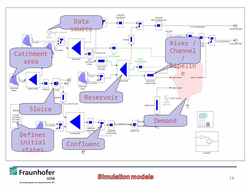
Catchmentarea

Defines initial states

Data source

River /Channel / Pipeline

Sluice

Confluence

Reservoir

Demand

11

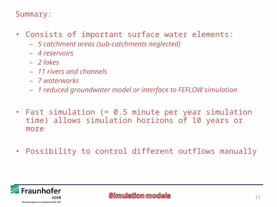
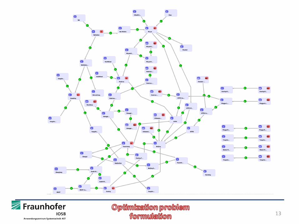
Summary:

• Consists of important surface water elements:– 5 catchment areas (sub-catchments neglected)– 4 reservoirs– 2 lakes– 11 rivers and channels– 7 waterworks– 1 reduced groundwater model or interface to FEFLOW simulation

• Fast simulation (≈ 0.5 minute per year simulation time) allows simulation horizons of 10 years or more

• Possibility to control different outflows manually

12

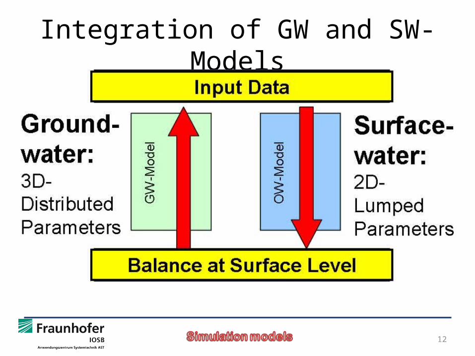
Integration of GW and SW-Models

13

14

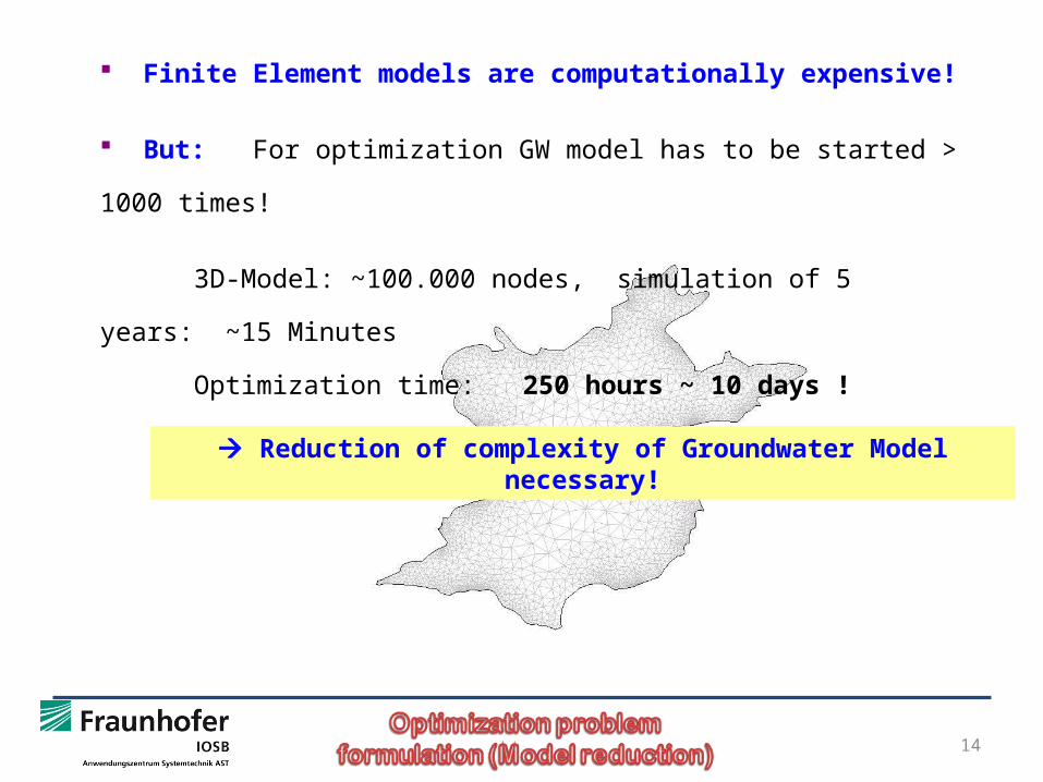
Finite Element models are computationally expensive!

But: For optimization GW model has to be started > 1000 times!

3D-Model: ~100.000 nodes, simulation of 5 years: ~15 Minutes

Optimization time: 250 hours ~ 10 days !

Reduction of complexity of Groundwater Model necessary!

15

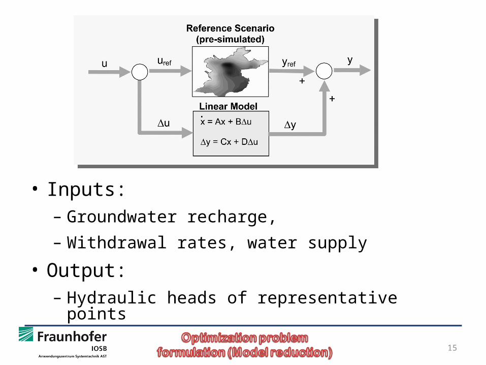
• Inputs: – Groundwater recharge, – Withdrawal rates, water supply

• Output:– Hydraulic heads of representative points

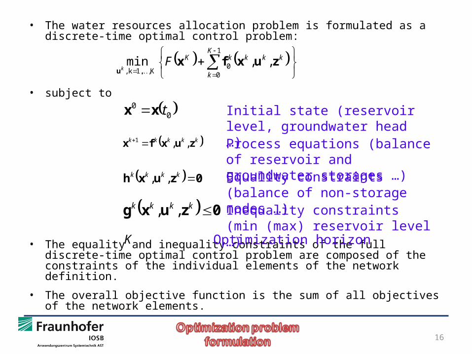
• The water resources allocation problem is formulated as a discrete-time optimal control problem:

• subject to

• The equality and inequality constraints of the full discrete-time optimal control problem are composed of the constraints of the individual elements of the network definition.

• The overall objective function is the sum of all objectives of the network elements.

16

1

00

K,1,k , ,, min

K

k

kkkkKFk

zuxfxu

00 txx

kkkkk zuxfx ,,1

0zuxh kkkk ,,

0zuxg kkkk ,,

Initial state (reservoir level, groundwater head …)Process equations (balance of reservoir and groundwater storages …)Equality constraints (balance of non-storage nodes …)Inequality constraints (min (max) reservoir level …)

Optimization horizonK

17

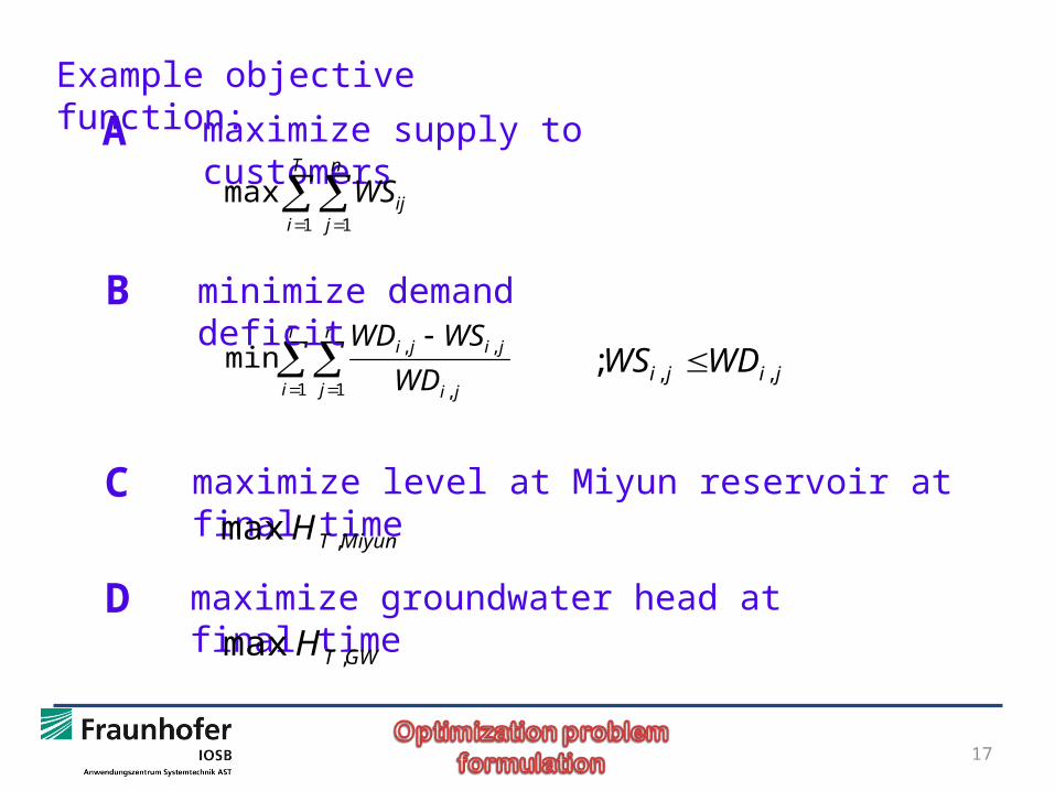
Example objective function:

A

B

C

D

maximize supply to customers

T

i

n

j ji

jiji

WD

WSWD

1 1 ,

,,min

T

i

n

jijWS

1 1

max

minimize demand deficit

maximize level at Miyun reservoir at final time

maximize groundwater head at final time

MiyunTH , max

GWTH , max

jiji WDWS ,, ;

18

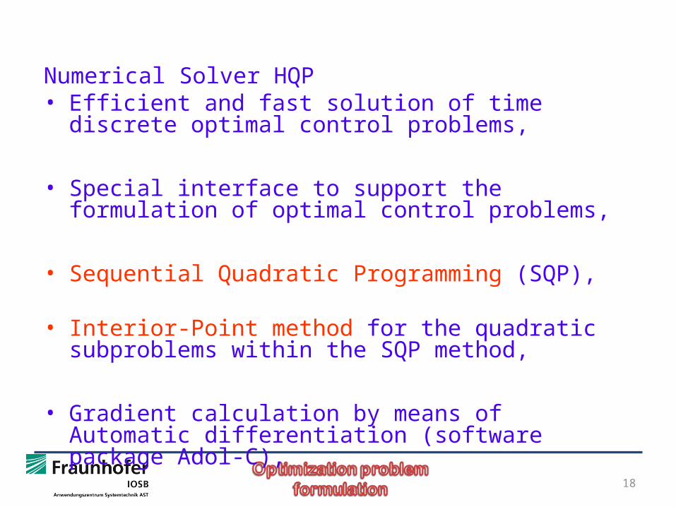
Numerical Solver HQP• Efficient and fast solution of time discrete optimal control

problems,

• Special interface to support the formulation of optimal control problems,

• Sequential Quadratic Programming (SQP),

• Interior-Point method for the quadratic subproblems within the SQP method,

• Gradient calculation by means of Automatic differentiation (software package Adol-C),

19

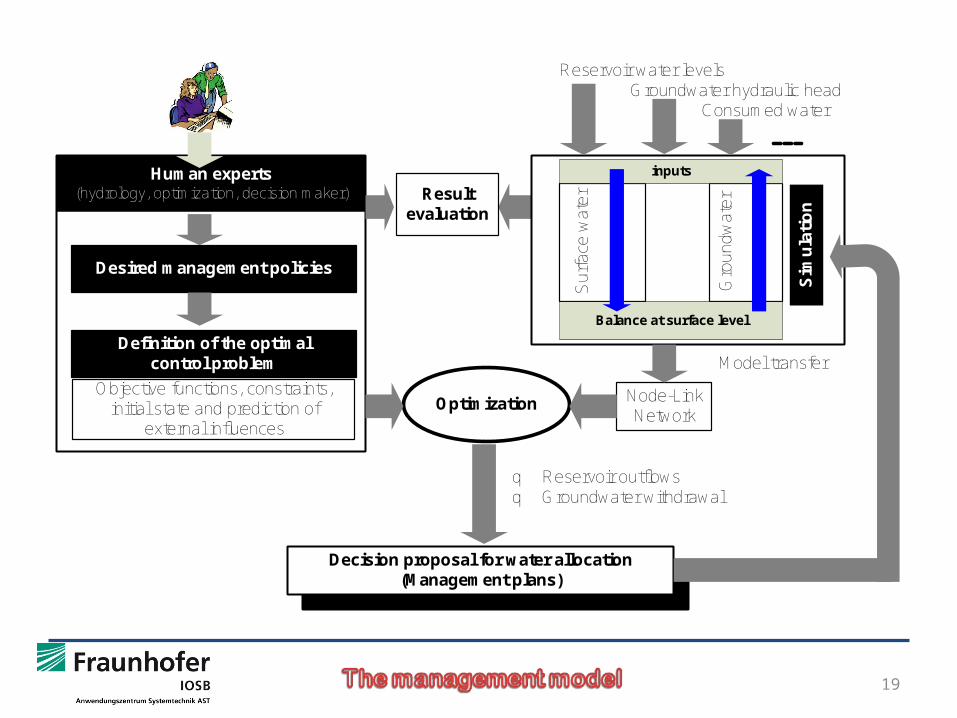
Decision proposal for water allocation(Management plans)

q Reservoir outflowsq Groundwater withdrawal

Reservoir water levelsGroundwater hydraulic head

Consumed water

Resultevaluation

Definition of the optimal control problem Model transfer

Sur

face

wat

er

Gro

undw

ater

Sim

ula

tio

n

Node-LinkNetwork

Human experts(hydrology, optimization, decision maker)

Objective functions, constraints, initial state and prediction of

external influences

Optimization

Balance at surface level

inputs

Desired management policies

20

Sim

ula

tio

nO

pti

miz

atio

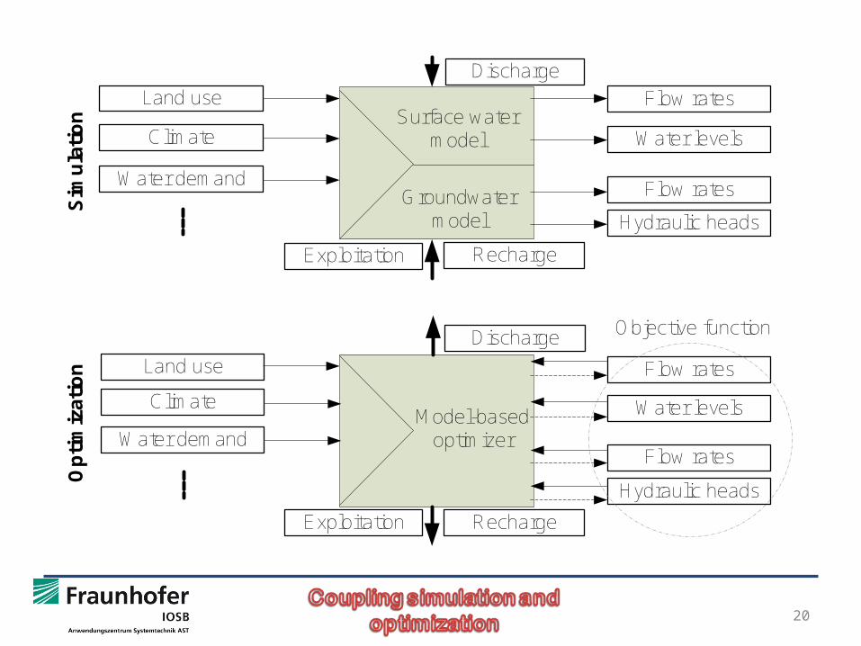
nLand use

Climate

Water demand

Flow rates

Flow rates

Water levels

Hydraulic heads

Flow rates

Water levels

Hydraulic heads

Flow rates

Land use

Climate

Water demand

Exploitation Recharge

RechargeExploitation

Discharge

Discharge

Objective function

Surface watermodel

Groundwatermodel

Model-basedoptimizer

21

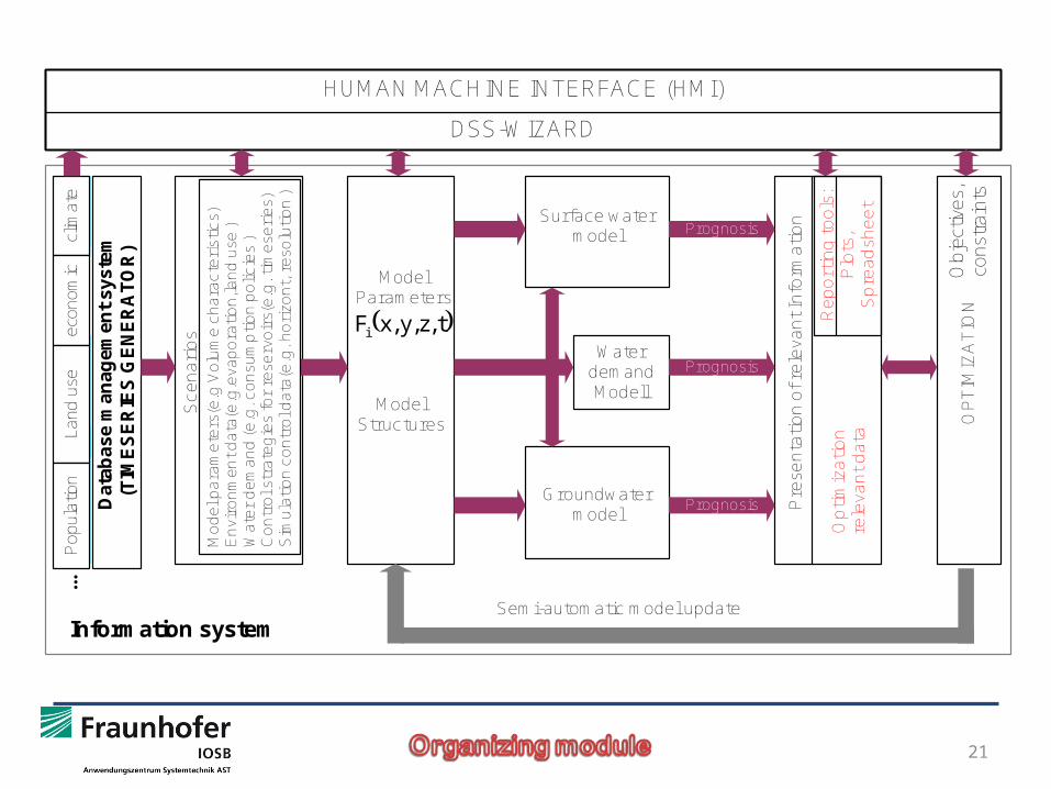
HUMAN MACHINE INTERFACE (HMI)

DSS-WIZARD

Prognosis

Prognosis

ModelParameters

ModelStructures O

PTIM

IZA

TIO

N

Pre

senta

tion o

f re

leva

nt In

form

ationSurface watermodel

Groundwater model

Scenari

os

clim

ate

econ

om

icLa

nd u

seP

opu

latio

n...

Report

ing tools

:P

lots

, S

pre

adsh

eet

Semi-automatic model update

Water demand Modell

Optim

ization

rele

vant data

Model p

ara

mete

rs(e

.g V

olu

me c

hara

cte

rist

ics)

Envi

ronm

ent data

(e.g

.eva

pora

tion,la

nd u

se )

Wate

r dem

and (e.g

. consu

mption p

olic

ies

)C

ontr

ol s

trate

gie

s fo

r re

serv

oir

s(e.g

. tim

ese

ries)

Sim

ula

tion c

ontr

ol d

ata

(e.g

. hori

zont,

reso

lution )

Prognosis

Information system

Dat

abas

e m

anag

emen

t sy

stem

(T

IME

SE

RIE

S G

EN

ER

AT

OR

)

Obj

ectiv

es,

cons

trai

nts

tz,y,x,Fi

22

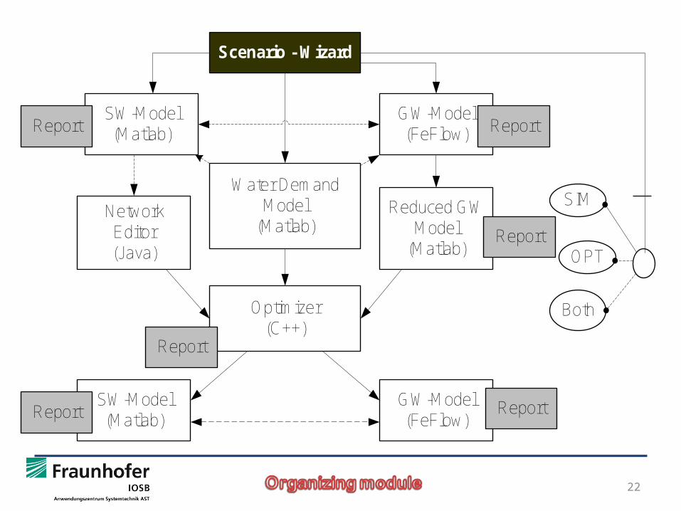
Scenario - Wizard

Water DemandModel

(Matlab)

Optimizer(C++)

SW-Model(Matlab)

GW-Model(FeFlow)

GW-Model(FeFlow)

Reduced GWModel

(Matlab)

SW-Model(Matlab)

Network Editor(Java)

Report

ReportReport

SIM

OPT

Both

ReportReport

Report

23

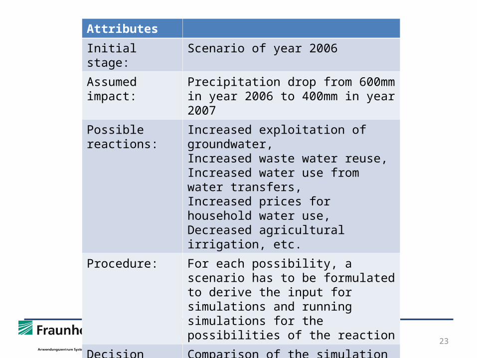
Attributes

Initial stage: Scenario of year 2006

Assumed impact: Precipitation drop from 600mm in year 2006 to 400mm in year 2007

Possible reactions: Increased exploitation of groundwater,Increased waste water reuse,Increased water use from water transfers,Increased prices for household water use,Decreased agricultural irrigation, etc.

Procedure: For each possibility, a scenario has to be formulated to derive the input for simulations and running simulations for the possibilities of the reaction

Decision support: Comparison of the simulation results and finding an optimum between the possibilities for a given goal function

Goal function: e.g., No limitations in water supply of the households and minimal costs.

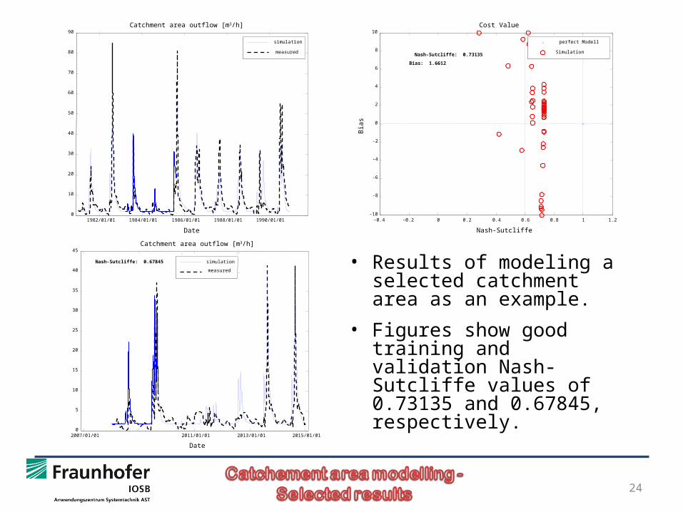
• Results of modeling a selected catchment area as an example.

• Figures show good training and validation Nash-Sutcliffe values of 0.73135 and 0.67845, respectively.

24

1982/01/01 1984/01/01 1986/01/01 1988/01/01 1990/01/010

10

20

30

40

50

60

70

80

90

Date

Catchment area outflow [m3/h]

simulation

measured

-0.4 -0.2 0 0.2 0.4 0.6 0.8 1 1.2-10

-8

-6

-4

-2

0

2

4

6

8

10

Bias

Nash-Sutcliffe

Cost Value

Nash-Sutcliffe: 0.73135

Bias: 1.6612

perfect Modell

Simulation

2007/01/01 2011/01/01 2013/01/01 2015/01/010

5

10

15

20

25

30

35

40

45

Date

Catchment area outflow [m3/h]

simulation

measured

Nash-Sutcliffe: 0.67845

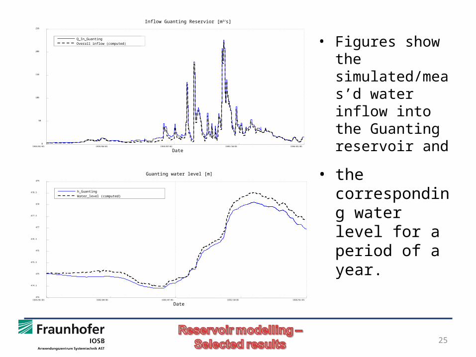
• Figures show the simulated/meas’d water inflow into the Guanting reservoir and

• the corresponding water level for a period of a year.

25

1995/01/01 1995/04/01 1995/07/01 1995/10/01 1996/01/010

50

100

150

200

250

Q_In_Guanting

Overall inflow (computed)

Date

Inflow Guanting Reservior [m3/s]

1995/01/01 1995/04/01 1995/07/01 1995/10/01 1996/01/01

474

474.5

475

475.5

476

476.5

477

477.5

478

478.5

479

h_Guanting

Water_level (computed)

Date

Guanting water level [m]

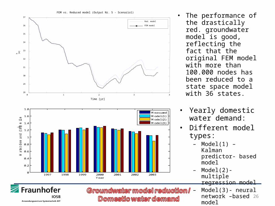
• The performance of the drastically red. groundwater model is good, reflecting the fact that the original FEM model with more than 100.000 nodes has been reduced to a state space model with 36 states.

26

0 1 2 3 428

29

30

31

32

33

34

35

36

37

Time [yr]

h [m]

FEM vs. Reduced model (Output Nr. 5 - Scenario1)

Red. model

FEM model

• Yearly domestic water demand:

• Different model types:

– Model(1) – Kalman predictor- based model

– Model(2)-multiple regression model

– Model(3)- neural network –based model

1997 1998 1999 2000 2001 2002 20030

0.2

0.4

0.6

0.8

1

1.2

1.4

1.6

1.8

Year

Wate

r dem

and (

100 m

il m

3 )

Measured

Model (1)Model (2)

Model (3)

• The proposed concept for optimal water management is evaluated for several sets of experiments.

• The first set of experiments compares two scenarios.

• Scenario 1:– minimize demand deficit and keep demand constant

for the next 10 years and

• Scenario 2 – minimize demand deficit and increase demand 5%

yearly for the next 10 years. The results of the two scenarios are illustrated in the Figures 4 to 5.

27

• Scenario 1 shows that the demand can be fulfilled for the ten years, but without considering sustainability, the Miyun reservoir and the Groundwater are overexploited.

• By increasing in Scenario 2 the demand yearly, then we can see that the demand won’t be fulfilled anymore

28

0 1 2 3 4 5 6 7 8 9 100

50

100

150

200

250

300

Time [y]

Beijing Water System - global demand and supply [m3/s]

global demand

global supply

Scenario 1

0 1 2 3 4 5 6 7 8 9 100

50

100

150

200

250

300

350

Beijing Water System - global demand and supply [m3/s]

global demand

global supply

Scenario 2

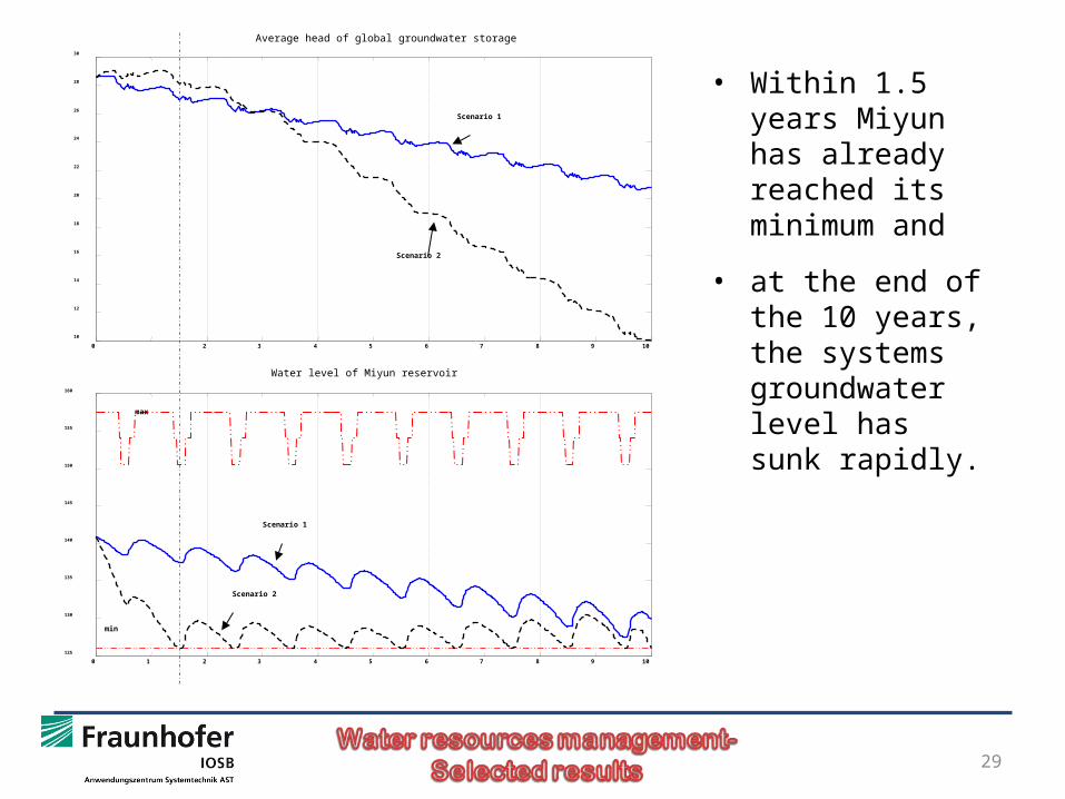
• Within 1.5 years Miyun has already reached its minimum and

• at the end of the 10 years, the systems groundwater level has sunk rapidly.

29

0 2 3 4 5 6 7 8 9 10

10

12

14

16

18

20

22

24

26

28

30

Average head of global groundwater storage

0 1 2 3 4 5 6 7 8 9 10

125

130

135

140

145

150

155

160

Water level of Miyun reservoir

Scenario 1

Scenario 2

Scenario 1

Scenario 2

max

min

30

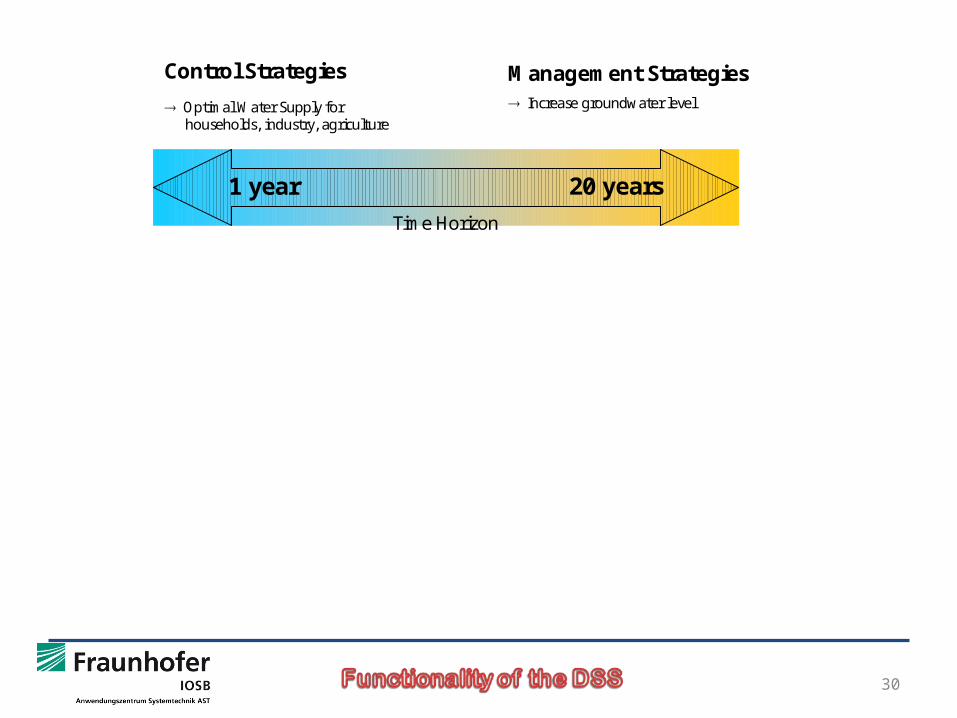
Control Strategies

Optimal Water Supply for households, industry, agriculture

1 year 20 years

Time Horizon

Management Strategies Increase groundwater level

• Management of water supply based on optimization

– optimized management of water resources

– optimized supply in periods of increased demand

– priority management in water scarcity periods

• Emergency management and water resources protection in case of

– natural disasters, terroristic attacks, accidents,

– water resources pollution

• Optimized adaptation of the water supply system to trends and changes

– evaluation and implementation of political decisions

– adaptation to changes in economy, population and agriculture

– handling climate changes and water quality degradation

– evaluation of increased waste water reuse

– strategies for sustainability of water use

• 4. Support for planning tasks

– simulation and optimization of future technical structures

– simulation and evaluation of resource recharge strategies

– simulation and evaluation of strategies of demand reduction

31

• Developed to meet the growing demands and pressures on water resources managers.

• Approach is state of the art and generic

• Based on a node-link network representation of the water resource system being simulated

• Include scenario planning in combination with state-of-the-art large-scale network flow optimization algorithm

• Places demand-side issues and water allocation schemes on an equal footing with supply-side topics

• Integrated approach to simulating both natural and man-made components of water systems

• Planner access to a more comprehensive view of the broad range of factors for sustainable water management

• GUI that facilitate user interaction and stresses out user sovereignty

32

Thank you for your attention !

Questions?

33