Embed Size (px)
Citation preview
Wesleyan University The Honors College
A Simulation of Circuit Creation in Tor
by
William Boyd
A thesis submitted to thefaculty of Wesleyan University
in partial fulfillment of the requirements for theDegree of Bachelor of Arts
with Departmental Honors in Computer Science
Middletown, Connecticut April, 2011

Acknowledgements
I would like to acknowledge my advisers, professors Norman Danner and Danny
Krizanc, for their help and guidance at all levels, from narrowing a huge range
of distance metrics to minor details of LATEX. Researching and writing this thesis
has been a formative experience, and you’ve been a major part of that; thank you.
I would also like to acknowledge my friends and family, for supporting me
through this whole process. It’s been rocky at times, but you were always there
when I needed you; thank you.
ii

Abstract
This thesis presents an accurate simulation of the circuit creation behavior of
the anonymity network Tor. Systems of all types are subject to attacks, which
must often be tested in simulation; many simulations do not accurately model
the behavior of the target network, making it difficult to discern which attacks
are of greatest concern. We simulate the circuit creation behavior of Tor using
hidden Markov models trained to the observed behavior of the real network. We
first observe the behavior of the network by probing individual routers; we then
cluster those observations into a few smaller observation sets, and train a hidden
Markov model from each cluster. We show by a probabilistic evaluation that our
model accurately simulates the behavior of Tor.
iii
Contents
List of Figures vi
List of Tables vii
Chapter 1. Introduction 1
1.1. Anonymity 1
1.2. Tor 3
1.3. Attacks on Tor 4
1.4. Contributions of this thesis 5
Chapter 2. Review of existing literature 7
2.1. Other simulations of Tor 7
2.2. Hidden Markov models 11
2.3. Clustering algorithms 13
2.4. Simulation credibility metrics 13
Chapter 3. Router lifecycles as a basis for circuit creation simulation 15
3.1. Observing router behavior 16
3.2. Router probe/circuit creation correlation 17
3.3. Router lifecycles 18
Chapter 4. Lifecycle clustering 19
4.1. Justification for clustering 19
4.2. Metrics on lifecycle sequences 20
iv

4.3. Clustering algorithms 23
Chapter 5. Hidden Markov models of lifecycles 27
5.1. Formal definition of hidden Markov models 27
5.2. Generation of hidden Markov models 28
Chapter 6. Model quality evaluation 34
6.1. Assumptions of our model 35
6.2. Numerical ratings 36
Chapter 7. Results 39
Chapter 8. Conclusion 42
Bibliography 44
v
List of Figures
4.1 Pseudocode for k-means approximation with Lloyd’s algorithm 24
4.2 Pseudocode for hierarchical agglomerative clustering 26
5.1 Pseudocode for the forward algorithm 30
5.2 Pseudocode for HMM generation 33
7.1 Expected model behaviors 40
vi

List of Tables
3.1 Results of router and circuit probes 17
7.1 Model ratings 41
vii
CHAPTER 1
Introduction
The modern Internet evolved from early experimental networks composed
mostly of small numbers of academic institutions. Early network engineers were
concerned primarily with ensuring that systems worked and were robust; privacy
and security were secondary concerns, if they received any consideration at all
[11]. The result of this evolution is that IP, the protocol over which the Internet
runs, is fundamentally non-anonymous; all the parties involved in any communi-
cation over IP know (down to network address) the identity of all other parties.
This makes the protocol simple and robust. However, the Internet has expanded
far beyond its open, academic origins. It is heavily used by parties such as polit-
ical dissidents, for whom being personally associated with their communications
is a dangerous liability, and other parties who value their privacy and anonymity.
Thus, a number of systems have been developed to sit on top of IP and anonymize
communications. These systems are subject to a variety of attacks; in lieu of ac-
tually attacking the system in question, it is often necessary to develop a suitable
simulation in order to test proposed attacks. This thesis develops such a sim-
ulation for one aspect of the behavior of a commonly-used anonymity system,
Tor.
1.1. Anonymity
Anonymity is the property of communications whereby they cannot be as-
sociated with a particular correspondent. In anonymity research, it is usually
1
1. INTRODUCTION 2
expressed as a degree in terms of the size of anonymity sets—that is, the smallest
set of potential correspondents an attacker can associate with a given message.
Anonymity systems were first seriously proposed by David Chaum in his sem-
inal 1981 paper [4]. Chaum proposed a series of computers termed “mixes” which
would use encryption to prevent attackers from correlating messages by the data
they contained and would reorder messages passing through them to prevent at-
tackers from correlating messages by time or order of entry into the network.
Chaum’s hypothetical mixes used layered public-key encryption to ensure that
messages would remain unintelligible to all but the last mix in a series: the client
would encrypt the message with the last mix’s public key, and then the second-
to-last’s, et cetera, until the outer layer of encryption could only be decrypted by
the first mix in the series. Each mix would then remove its layer of encryption,
until the last mix removed the last layer and revealed the original message, to be
passed to the recipient.
Nearly all modern anonymity systems are based on Chaum’s mix model,
though the specifics often vary widely. High-latency remailers such as Mixminion
[6] behave very similarly to Chaum’s proposed mixes: they collect, batch and
reorder messages before sending them on to the next mix in a series. These sys-
tems introduce a great deal of latency in the batch step as they wait for enough
messages to fill the batch; Mixminion, for example, has an average latency of ap-
proximately four hours [18]. This is clearly unsuitable for the interactive activities
which make up a significant portion of activity on the Internet.
Because of this unsuitability, much recent research and development has gone
into low-latency systems which forgo the batching step (and thus much of the
resistance to timing correlation attacks) in order to deliver average latencies on the
order of hundreds of milliseconds. Such systems may be used for web browsing,
1. INTRODUCTION 3
interactive remote shells, or other activities which require low latencies. One
widely-used decentralized low-latency anonymity system is Tor.
1.2. Tor
Tor is a low-latency anonymizing mix network [9]. As with Chaum’s proposed
mix networks, it sends client messages on a client-selected route through a network
of routers, layering encryption such that the origin and destination of a message
cannot be determined by any single participant other than the client. The goal
of Tor is to provide relatively strong anonymity while being easy to both use as
a client and support by running a router. In particular, it does not try to pro-
tect against global adversaries which can monitor or intercept all communications
through the network.
Tor consists of a network of onion routers which forward connections, and
is accessed by users using an onion proxy. Directory servers maintain a list of
routers which are currently in the network; there are few (as of this writing, nine)
authoritative directories which vote to form a consensus list of the routers in the
network. When users wish to send a connection through Tor, their proxy selects
three routers (an entry, middle, and exit router in that order) from the consensus
and builds a Tor circuit through them. Circuits are stateful and persistent; that
is, each router remembers the circuits passing through it. Stateful circuits pro-
vide several benefits over traditional onion routing as described by Chaum: they
eliminate the routing onion from messages, which allows the size of each message
to be normalized, and they allow individual segments to negotiate fast tempo-
rary symmetric encryption keys, rather than maintaining persistent but slow and
expensive public keypairs. All the data within a circuit is encrypted such that
only the router intended to receive a particular message can decrypt and read it.
1. INTRODUCTION 4
Additionally, the stateful routing means that each router knows only the routers
before and after it in a sequence, and so no single router can determine both the
start and endpoints of a circuit.
Once the proxy has built a circuit, it multiplexes TCP streams over the circuit.
The proxy sends instructions through the circuit to the last router to open a TCP
connection to the desired host. TCP packets traveling in both directions are then
grouped into fixed-length Tor cells and forwarded through each router; the last
router in the sequence unpacks data from the cells into TCP packets and sends
it to the corresponding host. Individual circuits have a relatively long default
persistence time of ten minutes.
1.3. Attacks on Tor
There are a wide variety of attacks on Tor, though most fall into one of two
categories. Short-term correlation attacks attempt to correlate messages going
into and out of the network based on patterns in traffic metadata, particularly
timing patterns in the delays between messages. This exploits the fact that Tor
attempts to minimize internal latency and thus may tend to preserve timing pat-
terns. It is generally assumed that Tor is vulnerable to timing attacks, and there
has been research which suggests this is in fact the case [16]; however, research
to confirm this is currently lacking. Most other attacks are variations on the
long-term anonymity set intersection attack which identifies a particular pair of
correspondents in multiple anonymity sets and takes the intersection of all those
sets to confirm that that particular pair is corresponding. Several articles pre-
senting varied attacks are presented in Chapter 2.
1. INTRODUCTION 5
1.4. Contributions of this thesis
Most proposed attacks on anonymity systems are demonstrated using a sim-
ulation of the target system. These simulations tend to be ad-hoc and often of
dubious veracity or correlation to the behavior of the real-world systems they are
meant to model. They tend to make sweeping simplifications, and the choice of
model is seldom justified. The simulations used in several articles are examined
in Chapter 2. There has been no work specifically on creating a high-quality,
valid simulation of any particular real-world anonymity system. Thus, we have
limited knowledge of how potentially dangerous any particular proposed attack
is, and consequently relatively little indication of the most productive directions
for future research.
The purpose of this thesis is to present and justify a robust and valid simulation
of circuit creation in Tor, upon which can be built simulations of other aspects
of the extant network; stream behavior and latency are obvious next targets for
simulation. We produce our model as follows:
(1) We observe router uptime/downtime behaviors.
(2) We cluster these observations into a few distinct categories.
(3) We simulate each category with a hidden Markov model.
This thesis is organized as follows. In Chapter 2, we provide a review of exist-
ing literature relevant to our subject. In Chapter 3, we discuss and justify router
lifecycles and our mechanism for observing them. In Chapter 4, we discuss clus-
tering lifecycles and various distance metrics and clustering algorithms used to
do so. In Chapter 5, we examine hidden Markov models and the algorithms to
manipulate and generate them. In Chapter 6, we consider techniques for com-
parison of our model to the real network it simulates. In Chapter 7, we give the

1. INTRODUCTION 6
results of our comparison of our model and Tor, and in Chapter 8, we present our
conclusions.
CHAPTER 2
Review of existing literature
Little literature has yet been written specifically about simulating any par-
ticular aspect of the Tor network, and none of it attempts to model the extant
network, instead modeling certain aspects of the Tor software’s behavior. Most
attack and defense papers test their proposed procedures on simulations of vary-
ing complexity; several standout examples are surveyed here. More useful to us,
however, are papers describing and justifying the techniques we use. To that end,
we will briefly review some literature on hidden Markov models, their use and
techniques for manipulating them; a survey of clustering algorithms; and several
papers on generalized simulation credibility criteria.
2.1. Other simulations of Tor
Most papers which propose an attack on Tor, some other real system, or even
a generalized system, simulate their attack on some sort of model to confirm
that the attack is practicable. These models are generally ad-hoc, and range
from simple random distributions of traffic and connections to more sophisticated
models taking into account assumptions about or measurements of likely actual
behaviors. We review the simulations used by three papers which use relatively
sophisticated models.
2.1.1. Danner et al. in an unpublished work produced a simulation of circuit
creation in Tor [7] to test the defense against active denial-of-service attacks they
proposed in a published version [8]. The attack they defend against, proposed by
7
2. REVIEW OF EXISTING LITERATURE 8
Borisov et al. [3], is an improvement on passive timing correlation by selectively
dropping uncontrolled connections. The authors showed that this attack can be
detected in a small number of circuit-testing probes, and tested their detection
algorithm both on the actual Tor network (concluding that the attack was not in
use at that time) and a simulation.
The simulation forms both the basis of and motivation for this thesis. The au-
thors attempted to create a circuit through each router in the consensus, recording
if the router succeeded or failed in the circuit creation, and tracked when routers
entered and exited the consensus with repeated probes over a period of time. This
forms the basis of the lifecycle model of router behavior we use. The authors as-
sumed that the distribution of states for a given router was probably time-based,
so they simulated router behavior by taking each state sequence for a given router
and rotating it by a random number of observations. Then the simulated router’s
behavior was determined by the lifecycle state at that time: if the observation
was a successful circuit creation, the simulated router would succeed in creating
the circuit; if the observation was a failed circuit creation, the simulated router
would fail; otherwise the simulated router would be out of the consensus.
This model of circuit creation matches the actual behavior of the Tor network
quite well. It obviously precisely matches the gross statistical behavior of the
network when the observations were actually made, and it preserves temporal
non-uniformities in router behavior (e.g., routers which go down every night).
However, we may expect that independent rotations are unrealistic; furthermore,
the simulation also has relatively fixed behavior (for instance, every router is up
the same fraction of the time), and so is subject to analyses that the more complex
behavior of the actual network defies; and it is incapable of producing more data
than was originally recorded.

2. REVIEW OF EXISTING LITERATURE 9
2.1.2. Levine et al. in 2004 presented a generalized timing attack on low-
latency mix-based anonymizing systems [13]. They describe an attack in which
the attacker measures the number of packets which pass through a given link in a
given period of time and then attempt to correlate that with similar measurements
of another link. The also propose a defense against the attack by selectively
dropping packets to obfuscate the timing signatures. They then implement their
attack and defense on a simulated network.
Their model is of a general low-latency mix system, rather than specifically
Tor, but they make reasonable assumptions about the structure of such a system.
In particular, they produce two general models of individual nodes: a low-latency
server mix model in which the mixes are assumed to be dedicated servers, and a
high-latency peer mix model in which the mixes are assumed to be low-bandwidth,
inconsistent network peers. Packet drop rates follow a normal distribution, with
low mean and small standard deviation for server mixes and high mean and large
standard deviation for peer mixes. Latencies were selected uniformly from a small
range for servers and by following an experimentally derived distribution for peers.
Paths through the network were selected randomly, with a length selected uni-
formly from a range.
This network model is unusually sophisticated and is particularly notable for
justifying most of the parameters it uses with observations and experiments. How-
ever, the model fails to account for the behavior of the mixes themselves, rather
than the links between them. Thus, every mix is active and accepting traffic at
all times, which we observe later is an unrealistic assumption for Tor. Routing of
data through the mix is also handled in a very generalized way which does not
match Tor’s behavior.
2. REVIEW OF EXISTING LITERATURE 10
The model of user traffic over the network was also particularly well-considered,
though less relevant to our problem. The authors used a variety of models, in-
cluding recordings of actual user activity, random normally-distributed activity,
and some others; they noted that some of their models did not match reasonable
assumptions about user behaviors, but wanted a variety of gross behaviors on
which to test their attacks and defenses.
2.1.3. Mathewson and Dingledine in 2004 extended an earlier proposed long-
term intersection attack called the statistical disclosure attack [5] to more effec-
tively cope with realistic assumptions about user behavior [15]. The attacker
accumulates data about the victim’s possible correspondents over a given period
of time, and uses these data to restrict the set of possible correspondents until she
can confirm the victim’s correspondent set.
To test the attack, the authors produced a variety of models of increasing
complexity. The initial model took the entire mix as a black box and a single round
of observation as atomic; thus, the network itself was entirely hypothetical (for
example, there was no latency). Only the behavior of the users of the network was
modeled, as a uniform selection of correspondents out of some set. Later models
increased the complexity of the simulated user behavior (for example, by selecting
correspondents according to a simulated social network rather than uniformly).
The most complex models used a pool mix, where some messages are main-
tained in the mix over observation rounds, rather than a simple threshold mix
in which every message is forwarded in the batch in which it is received. This
network model is still unrealistic; real mix networks drop messages and behave in
other unpredictable and non-ideal ways.

2. REVIEW OF EXISTING LITERATURE 11
This sort of model, with the network itself taken to be unrealistically ideal, is
common among simulations of proposed attacks. Indeed, the prevalence of such
models serves to motivate this thesis.
2.2. Hidden Markov models
Hidden Markov models (HMMs) are widely used in a variety of fields to model
probabilistic processes. Rabiner’s 1989 tutorial [17] is still considered to be the
definitive introduction to the topic.
Rabiner opens with a description of HMMs. An HMM is a Markov process
in which states emit observations according to a probability distribution, rather
than deterministically; that is, the actual states are hidden. Hence we have a set
of states, a state transition probability distribution, an observation probability
distribution for each state, and a starting state probability distribution. From
this, it is straightforward to generate sample observation strings; we just prob-
abilistically select a start state, follow a state sequence and select observations
from each given state in the sequence.
Rabiner presents three basic problems for handling HMMs. These are problems
which must be solved to manipulate HMMs in useful ways; in particular, they deal
with transitioning from observed strings to HMMs. The problems are:
(1) Given an observed sequence and a preexisting model, what is the proba-
bility that the model generated the observation?
(2) Given an observed sequence and a preexisting model, what is the most
likely sequence of states within the model to have generated the observa-
tion?
(3) Given an observed sequence, what HMM is most likely to have generated
the observation?
2. REVIEW OF EXISTING LITERATURE 12
These three basic problems build on each other. We are particularly interested in
solutions or approximations of the third problem, since we wish to produce HMMs
to serve as models of actual systems giving observed sequences.
Rabiner first gives an exact solution to the first problem, of calculating the
probability of a given sequence from a given model. The probability is derived
as the sum of the probability of a given observation sequence from a given state
sequence over all possible state sequences. Calculating this directly is infeasible,
as there are an exponential number of possible state sequences of a given length,
but Rabiner describes the forward algorithm, an efficient dynamic programming
algorithm to find the exact probability.
The second problem is similarly intractable when approached naıvely; since
there are an exponential number of state sequences of a given length, enumerat-
ing them all and selecting the one most likely to produce the given sequence is
infeasible. Instead, Rabiner presents the Viterbi algorithm, which builds on the
forward algorithm to efficiently determine the most probable state sequence.
The third problem has no known efficient exact solution. Rabiner describes
a particular optimization method based on work of Baum et al. [2] to search for
high quality models of a particular sequence; however, given the solutions to the
first and second problem, this problem is likely subject to analysis by a variety of
general optimization heuristics.
Rabiner goes on to describe some particular special cases of HMMs, such as
models which do not allow state regression, models for continuous observed phe-
nomena, and some other cases which are not relevant to our problem. The tutorial
then presents a basic similarity measure for HMMs which compares observation
sequences generated by one model against another; it goes on to describe the
2. REVIEW OF EXISTING LITERATURE 13
use of HMMs in the particular case of speech recognition, which is again largely
irrelevant to us.
2.3. Clustering algorithms
As with HMMs, clustering algorithms have wide applicability across a vari-
ety of fields. Xu and Wunsch in 2005 produced a definitive survey of clustering
algorithms [19] which we use. The authors describe a wide variety of cluster-
ing algorithms for data ranging from numbers, vectors, strings, up to clustering
bodies of literature. We are interested primarily in simple and robust clustering
algorithms for relatively small strings of observations; Xu and Wunsch describe in
particular k-means and hierarchical clustering, two such algorithms that we use.
2.4. Simulation credibility metrics
In the field of simulation studies, the validity of models is a subject of consid-
erable concern. Significant recent research has gone into analyzing the method-
ologies and metrics used to assess the credibility and validity of simulations [14].
Unfortunately, there is little work yet to validate a mathematical model as a
preferable (or even “good”) simplification of a poorly-understood system. We use
the handbook edited by Banks [1] as our reference; the handbook discusses all
aspects of simulation studies, in particular the credibility-determining process of
verification, validation and accreditation (VVA).
Verification is the process of ensuring that the model is implemented correctly;
validation is the process of ensuring that the model is a good choice at all; and
accreditation is gained through third-party oversight. Verification and accredita-
tion are well-understood and developed; unfortunately, validation is not, and it

2. REVIEW OF EXISTING LITERATURE 14
is this aspect of simulation credibility which mostly concerns us. Banks’s hand-
book describes validation as a process of qualitatively examining assumptions and
selecting statistical tests which seem applicable. We wish to avoid this level of
subjectivity in validity assessment, and so believe further research in the field is
warranted.

CHAPTER 3
Router lifecycles as a basis for circuit creation simulation
We wish to model the behavior of Tor with respect to circuit creation. There
are many possible circuits; at any given time, there are approximately 2500 routers
in the Tor consensus, of which approximately 1000 are exit routers, so there are in
excess of 6 billion possible three-router circuits. This is far too many to reasonably
test directly, especially since the set of routers in Tor itself is constantly changing
and so we may expect the set of possible circuits to change significantly while we
are examining it. Thus, we simplify the problem: we demonstrate that circuit
creation behavior is strongly correlated with the behavior of individual routers
within each circuit, and then reduce our problem to one of simulating router
behavior. Since there are many fewer routers than possible circuits, this problem
is tractable.
We model routers as either successfully creating a circuit or failing to create
a circuit when requested1. Thus, we produce a binary alphabet describing the
circuit creation behavior of routers:
• Success. This router will successfully allow circuits to be built through
it.
• Failure. The router will not allow circuits to be built through it; it may
have fallen out of the Tor consensus, it may be unreachable from the
onion proxy’s perspective, it may have gone offline and not yet timed out
of the consensus, or it fails circuit creation for some other reason.
1More complex simulations, such as dealing with latency, may want to differentiate betweendifferent failure conditions.
15

3. ROUTER LIFECYCLES AS A BASIS FOR CIRCUIT CREATION SIMULATION 16
Thus for any given router at any given point, we may succinctly describe its
behavior according to a particular known alphabet.
Given observations of three routers g, m and e at a particular time, we wish to
predict that the circuit 〈g,m, e〉 through those three routers will succeed exactly
when each of g, m and e exhibit success at that time; if any router in a circuit
fails, we predict that the circuit will also fail.
To examine this model, we first probe each router in the Tor consensus once
to acquire an observation of its behavior. We then attempt to build a number of
circuits, observing whether the circuit creation succeeds or fails.
3.1. Observing router behavior
We observe the routers over the entire network through the following proce-
dure:
(1) Determine the consensus, that is, the set R of routers reported to cur-
rently be accepting connections.
(2) For each router r in R, attempt to construct a circuit 〈g, r, e〉 through r
from an entry node g we control to an exit node e we also control (we
call this a probe of r).
(3) If the circuit construction succeeds, record success for r; otherwise record
failure.
Since we control g and e, we may be sure that any failures are due to the behavior
of r. This gives us an observation of the behavior of each router in the consensus
at a particular time. We then examine circuit creation behavior:
(1) Determine the consensus R.
(2) Attempt to build a circuit 〈g,m, e〉 using three routers g, m and e selected
at random from R.
3. ROUTER LIFECYCLES AS A BASIS FOR CIRCUIT CREATION SIMULATION 17
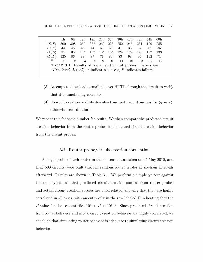
1h 6h 12h 18h 24h 30h 36h 42h 48h 54h 60h〈S, S〉 300 308 259 262 269 226 252 245 231 199 255〈S, F 〉 44 46 48 44 55 56 41 33 32 47 35〈F, S〉 31 60 105 107 105 135 124 124 143 122 139〈F, F 〉 125 86 88 87 71 83 83 98 94 132 71P −49 −26 −13 −14 −9 −6 −11 −16 −12 −12 −14Table 3.1. Results of router and circuit probes. Labels are〈Predicted, Actual〉; S indicates success, F indicates failure.
(3) Attempt to download a small file over HTTP through the circuit to verify
that it is functioning correctly.
(4) If circuit creation and file download succeed, record success for 〈g,m, e〉;
otherwise record failure.
We repeat this for some number k circuits. We then compare the predicted circuit
creation behavior from the router probes to the actual circuit creation behavior
from the circuit probes.
3.2. Router probe/circuit creation correlation
A single probe of each router in the consensus was taken on 05 May 2010, and
then 500 circuits were built through random router triples at six-hour intervals
afterward. Results are shown in Table 3.1. We perform a simple χ2 test against
the null hypothesis that predicted circuit creation success from router probes
and actual circuit creation success are uncorrelated, showing that they are highly
correlated in all cases, with an entry of x in the row labeled P indicating that the
P -value for the test satisfies 10x < P < 10x−1. Since predicted circuit creation
from router behavior and actual circuit creation behavior are highly correlated, we
conclude that simulating router behavior is adequate to simulating circuit creation
behavior.

3. ROUTER LIFECYCLES AS A BASIS FOR CIRCUIT CREATION SIMULATION 18
3.3. Router lifecycles
Since we wish to model the behavior of Tor over a period of time, it is necessary
to observe each router over a period of time. We call a single observation of each
router in the consensus a trial; in order to collect observations over time, we repeat
trials until we have the desired duration of data. If a router is in the consensus
only for some probes, it is considered to fail at all other probes. We call a series
of observations for a single router a lifecycle for that router.
We have now described and justified the procedure for observing network life-
cycles. We will next describe our methods for clustering lifecycles, and then
discuss the generation of hidden Markov models from lifecycle clusters.
CHAPTER 4
Lifecycle clustering
Clustering algorithms are used in a wide variety of contexts. They are often
used for exploratory analysis or to group large or complex datasets into meaningful
subsets for further study. We use clustering to group our observed router lifecycle
data into a manageable number of categories, in order to simplify the process of
generating the model and simplify the model itself with minimal impact on the
quality of generated outputs.
4.1. Justification for clustering
We expect routers to fall into a number of relatively well-defined categories;
for example, there are many routers which exhibit perfect uptime over the course
of an observation run, and some which exhibit regular uptime/downtime cycles
as their administrators take them offline at night or over weekends. Clustering
router lifecycles allows us to simplify our representation of the overall network
while remaining accurate to the behavior of the real Tor network. Furthermore,
we can perform some analysis of the state of the real network based on the clusters
we observe, and we can easily modify the network model to provide insight into
the behavior of the real network under various assumptions. If, for example,
we wanted to observe network behavior when high-profile router operators are
attacked or their routers blocked from access, we could reduce the proportion of
several high-uptime clusters in our overall model.
19

4. LIFECYCLE CLUSTERING 20
4.2. Metrics on lifecycle sequences
Clustering algorithms depend on some notion of “distance” between objects be-
ing clustered; thus, we need such a notion for sets of equal-length binary sequences
S. We use a distance metric, which is defined to be a function D : S × S → R
satisfying the following constraints:
• Symmetry; that is, D(x, y) = D(y, x).
• Positivity; that is, for all x, y we have D(x, y) ≥ 0.
• The triangle inequality; that is, for all x, y, z we have
D(x, y) +D(y, z) ≤ D(x, z).
• Reflexivity; that is, D(x, y) = 0 if and only if x = y.
Additionally, k-means clustering requires that we calculate a center of a set
of sequences under any given distance metric. We define this according to the
metric in question, since calculating a center according to a particular definition
may not be feasible under some metrics. In general, we wish for the center of a set
of sequences to minimize the sum of squared distances over the entire set, but we
will select centers according to reasonable, efficient behavior, not how well they
satisfy this criterion.
There are a number of reasonable candidate metrics for binary sequences.
We will present the ones we use here, and compare the results of using each in
Chapter 7.
4.2.1. Hamming distance. The simplest sequence distance metric, and one
that is very well understood and commonly used, is Hamming distance, defined to
be the number of characters at which two sequences differ [10]. Hamming distance
is simple and fast to calculate and is well-known to be a metric on same-length
sequences, so we will concern ourselves only with center-finding under it.
4. LIFECYCLE CLUSTERING 21
We define the center c of a set S of sequences under Hamming distance to be
the sequence which minimizes the sum of squared distances to all the sequences
in S. This is the sequence which agrees with the majority of the sequences in S
at each position independently, which may be easily shown by contradiction; if c
were the center but disagreed with the majority of the sequences in S at some
position, the sequence c′ which agreed with the majority at that position and with
c at all other positions would have lower total distance (because it agrees with
more sequences at that position without disagreeing with any others at any other
position) and thus a lower sum of squared distances, contradicting the centrality
of c.
4.2.2. Edit distance. Edit distance describes a number of related metrics,
such as Levenshtein distance [12], which indicate the minimum number of “ed-
its” to one sequence it would take to reach another. The different metrics have
different permissible edits. Levenshtein distance, for instance, allows insertion of
characters, deletion of characters, and changing one character into another (sub-
stitution). This is inappropriate for our purposes, since insertion and deletion of
observations from a lifecycle sequence is not meaningful; hence we use an alter-
nate edit distance metric in which the permitted operations are substitution and
characterwise rotation, to capture routers which have similar behavior but are
time-offset. We define characterwise rotation to be either left or right rotation,
where left rotation by d characters transforms each character si in a sequence S
into the character si+d (mod |S|), and right rotation transforms it into si−d (mod |S|).
We will consider three variations on this distance metric, depending on the
cost assigned to rotation.
(1) Rotation has zero cost. We call this distance metric E0. In this case,
distinct sequences are equivalent if they are rotations of one another;

4. LIFECYCLE CLUSTERING 22
thus, E0 is a metric on equivalence classes of sequences under rotation,
not on sequences themselves.
(2) Any degree of rotation has unit cost, so rotated sequences are not equiv-
alent but there is no difference between rotating by one character or by
arbitrarily many. We call this distance metric E1.
(3) Each character of rotation has unit cost. We call this distance metric E2.
We will call the class of all three edit distance variations E.
These edit distances can be shown to be distance metrics as follows.
• E is symmetric; if E(x, y) = n then there is some sequence of edit opera-
tions needed to transform x to y with total cost n. Since each operation
is reversible for the same cost, the reverse sequence of inverse edit oper-
ations will transform y to x also with total cost n, and will be minimal;
thus, E(y, x) = n.
• E is positive; it is the sum of the costs of a sequence of nonnegative-cost
edit operations.
• E obeys the triangle inequality. Consider three sequences x, y and z of
equal length. Let E(x, y) = n and E(y, z) = m. Then there is a sequence
of edit operations that can transform x to y with cost n and one that
can transform y to z with cost m. Thus, the combination of these two
sequences of edit operations can transform x through y to z with cost at
most n+m, so E(x, z) ≤ n+m.
• E is reflexive; if x and y are equal, then no edits are needed to go between
them, and so E(x, y) = 0; similarly, if E(x, y) = 0 then no edits are
needed to go between them and so they are equal (or equivalent in the
case of E0)
Hence E is a distance metric.
4. LIFECYCLE CLUSTERING 23
There is no clear way (under any of our costs for rotation) to efficiently de-
termine the sequence which minimizes the sum of squared distances over a set of
sequences under any of the edit distance metrics. Since k-means depends on a
stable center to converge, we cannot feasibly approximate the center of a set of ob-
servations; any variation in the approximated center would prevent the algorithm
from converging. Thus, we select centers by median: the center is the element
already present in the set which minimizes the sum of squares of distances to all
other elements in the set.
4.3. Clustering algorithms
There is a variety of clustering algorithms with differing behaviors, properties
and applications. In general, clustering algorithms seek to partition a set of ele-
ments into some number of clusters, minimizing the value of some discrimination
criterion function within each cluster. Under this broad umbrella, there are many
variations: hierarchical clustering algorithms which produce nested cluster hier-
archies, for example, or fuzzy clustering algorithms which assign elements degrees
of presence in each cluster, rather than discrete assignment. We wish to produce
discrete clusters of similar sequences and select an exemplar sequence from each.
We will consider two reasonable discrete clustering algorithms, k-means clustering
and hierarchical clustering, and compare the results of using each in Chapter 6.
We use these two clustering algorithms because they are simple, robust, and match
our needs.
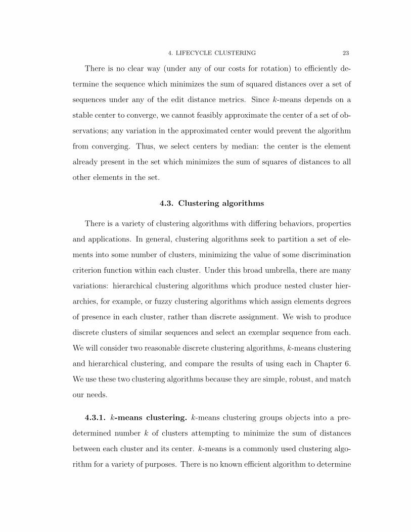
4.3.1. k-means clustering. k-means clustering groups objects into a pre-
determined number k of clusters attempting to minimize the sum of distances
between each cluster and its center. k-means is a commonly used clustering algo-
rithm for a variety of purposes. There is no known efficient algorithm to determine
4. LIFECYCLE CLUSTERING 24
function kmeans (X : set of binary sequences, k : integer) :list of sets of binary sequencesbeginZ: list of k binary sequencesC: list of k sets of binary sequencesfor i← 0 to k − 1 doZ(i)← a random unique element from X
end forfor x ∈ X doi← the i which minimizes D(x, Z(i))add x to C(i)
end forC ′: list of k sets of binary sequenceswhile C 6= C ′ do
for i← 0 to k − 1 doZ(i)← the center of C(i)
end forC ← C ′
for x ∈ X doi← the i which minimizes D(x, Z(i))add x to C ′(i)
end forend whilereturn C
end
Figure 4.1. Pseudocode for k-means approximation withLloyd’s algorithm
the optimal arrangement of items into clusters for k-means; however, the stan-
dard approximation algorithm, Lloyd’s algorithm, gives good results. In Lloyd’s
algorithm, initial centers are selected, and then items are assigned to the cluster
with the nearest center. New centers are selected for each cluster, items are again
assigned to the cluster with the nearest center, and the process is repeated until
it converges. Pseudocode for an implementation of Lloyd’s algorithm for binary
sequences under distance metric D is given in Figure 4.1.
4.3.2. Hierarchical clustering. Hierarchical clustering produces a nested
hierarchy of cluster membership; at the root of the hierarchy is a single cluster
4. LIFECYCLE CLUSTERING 25
containing every element, while the leaves are single-element clusters. We can
select arbitrary numbers of clusters by cutting the hierarchy tree at an appropriate
depth.
There are two main methods to generating a hierarchical clustering tree. Be-
ginning from the top with a single all-inclusive cluster and splitting to give smaller
clusters is termed divisive clustering; beginning from the bottom with unit clusters
and merging those which are close to give larger clusters is termed agglomerative
clustering. Divisive clustering tends to be very expensive (since there are an expo-
nential number of potential divisions of a given cluster to evaluate); agglomerative
clustering algorithms are more common in practice [19], and we use one.
It is necessary with agglomerative clustering to have a definition for some
notion of distance (not generally a metric) between two clusters. Many suitable
definitions exist; we use complete linkage distance, in which the distance between
any two clusters is the maximum distance of any two elements in them. That is,
given clusters X and Y , the complete linkage distance DC under distance metric
D is
(1) DC(X, Y ) = maxx∈X,y∈Y
D(x, y)
Complete linkage distance is simple and fast, and tends to result in dense, localized
clusters, a behavior we consider desirable.
Since we wish for only a particular number of clusters and do not need the
hierarchy above or below the tree at the point it has that many clusters, we
simply agglomerate clusters, discarding information about prior clusters until we
have reached the desired number of clusters. Pseudocode for the agglomerative
hierarchical clustering algorithm we use is given in Figure 4.2.

4. LIFECYCLE CLUSTERING 26
function hierarchical (X : set of binary sequences, k : integer) :set of sets of binary sequencesbeginC ← partition of singleton sets of Xwhile len(C) > k do
(c0, c1)← the unequal pair in C × C minimizing DC(c0, c1)remove c0, c1 from Cadd c0 ∪ c1 to C
end whilereturn C
end
Figure 4.2. Pseudocode for hierarchical agglomerative clustering
We have now described router lifecycle lifecycle observation and clustering.
In the next chapter, we will describe procedures for generating hidden Markov
models from lifecycle clusters.

CHAPTER 5
Hidden Markov models of lifecycles
Hidden Markov models are a commonly used statistical model for temporal
processes. They are a compact way to represent Markov processes, that is, discrete
processes which obey the Markov property: the behavior of the process at any
given point in time depends on at most a constant, finite amount of its past
state. Markov processes are the most complex stochastic processes easily analyzed,
and they can encompass most behaviors we expect to need (see Chapter 6). For
the complexity of the Markov processes we expect to work with, hidden Markov
models are the most reasonable representation.
5.1. Formal definition of hidden Markov models
Formally, an HMM consists of the following:
• A set Q of states with size N .
• An alphabet Σ of output symbols with size M .
• A state transition probability distribution function A : Q × Q → [0, 1]
giving the probability of a transition from one state to another. Since A
is a probability distribution, it must satisfy that for each q in Q we have∑x∈QA(q, x) = 1.
• An output symbol emission probability distribution function
B : Q× Σ→ [0, 1] giving the probability of a given symbol being ob-
served from a given state. B must satisfy that for each q in Q we have∑σ∈Σ B(q, σ) = 1.
27

5. HIDDEN MARKOV MODELS OF LIFECYCLES 28
• A start state probability distribution function π : Q → [0, 1] giving the
probability that a given state is selected as the first state in a sequence.
π must satisfy∑
q∈Q π(q) = 1.
An HMM may be used to generate an output string by selecting a sequence of
states according to π and A and from that generating an output according to B.
5.2. Generation of hidden Markov models
Generating a hidden Markov model is a heuristic optimization procedure.
There is no known algorithm for finding an optimal HMM of a given number
of states for a given string. We instead use local optimization to find a relatively
good local maximum of the model space for probability of generating the given
string.
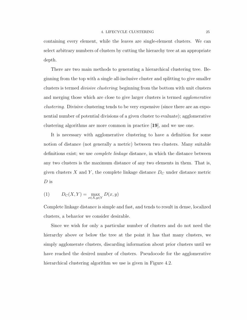
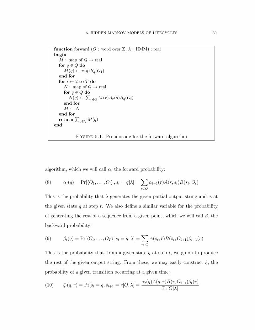
5.2.1. The forward algorithm. The forward algorithm is a dynamic pro-
gramming algorithm to determine the probability that a given HMM produces a
given output string. We take a given observation sequence O = 〈O1, O2, . . . , OT 〉
and a given HMM λ = 〈Q,Σ, A,B, π〉 and wish to calculate Pr[O|λ]. If we are
given a state sequence S = 〈s1, s2, . . . , sT 〉 over Q, then we may calculate the
probability of O given this state sequence:
(2) Pr[O|S, λ] =T∏i=1
B(si, Oi)
Furthermore, the probability of a given state sequence S is
(3) Pr[S|λ] = π(s1)T−1∏i=1
A(si, si+1)
Thus, the probability of O given only the model λ is then
(4) Pr[O|λ] =∑
all S of len T
Pr[O|S, λ] Pr[S|λ]
5. HIDDEN MARKOV MODELS OF LIFECYCLES 29
There are |Q|T such possible state sequences, so calculating this directly is infeasi-
ble for large models or observation sequences. Fortunately, since transition events
are independent, the probability of generating O depends only on the probability
of generating the first T − 1 letters of O ending with each possible state. That is,
for some given state q,
(5) Pr[O, sT = q|λ] =∑r∈Q
Pr[〈O1, . . . , OT−1〉 , sT−1 = r|λ] · A(r, q) ·B(q, OT )
and so
(6) Pr[O|λ] =∑q∈Q
Pr[O, sT = q|λ]
which suggests a dynamic programming algorithm to find Pr[O|λ], which we call
the forward algorithm. We use the inductive identity above and define the base
case:
(7) Pr[〈O1〉 , s1 = q|λ] = π(q)B(q, O1)
Pseudocode is given in Figure 5.1. This algorithm runs in time Θ(T · |Q|2).
5.2.2. The Baum-Welch algorithm. The Baum-Welch algorithm takes an
HMM and an output string and returns a nearby HMM which is more likely to
have generated that string, if the given HMM is not already at a local maximum in
the model space. The Baum-Welch algorithm was first presented and verified by
Baum et. al in 1970 [2]; we wish to generate HMMs which match sets of sequences
as well as possible, so we extend Baum-Welch to serve this purpose.
The algorithm produces a statistical re-estimation of the model parameters.
We first consider the inductive probability in Equation 5 used for the forward
5. HIDDEN MARKOV MODELS OF LIFECYCLES 30
function forward (O : word over Σ, λ : HMM) : realbeginM : map of Q→ realfor q ∈ Q doM(q)← π(q)Bq(O1)
end forfor i← 2 to T doN : map of Q→ realfor q ∈ Q doN(q)←
∑r∈QM(r)Ar(q)Bq(Oi)
end forM ← N
end forreturn
∑q∈QM(q)
end
Figure 5.1. Pseudocode for the forward algorithm
algorithm, which we will call α, the forward probability:
(8) αt(q) = Pr[〈O1, . . . , Ot〉 , st = q|λ] =∑r∈Q
αt−1(r)A(r, st)B(st, Ot)
This is the probability that λ generates the given partial output string and is at
the given state q at step t. We also define a similar variable for the probability
of generating the rest of a sequence from a given point, which we will call β, the
backward probability:
(9) βt(q) = Pr[〈Ot, . . . , OT 〉 |st = q, λ] =∑r∈Q
A(st, r)B(st, Ot+1)βt+1(r)
This is the probability that, from a given state q at step t, we go on to produce
the rest of the given output string. From these, we may easily construct ξ, the
probability of a given transition occurring at a given time:
(10) ξt(q, r) = Pr[st = q, st+1 = r|O, λ] =αt(q)A(q, r)B(r, Ot+1)βt(r)
Pr[O|λ]

5. HIDDEN MARKOV MODELS OF LIFECYCLES 31
And from this, we construct γ, the probability of the model being in a given state
at a given time:
(11) γt(q) =∑r∈Q
ξt(q, r) or∑r∈Q
ξt(r, q)
These variables provide the building blocks to produce a re-estimation of the model
parameters based on the expected fractions of starts, transitions and emissions.
We produce our new model parameters:
π(q) = γ1(q) = the likelihood q is the start state(12)
A(q, r) =
T−1∑t=1
ξt(q, r)
T−1∑t=1
γt(q)
= the fraction of transitions from q to r(13)
B(q, σ) =
T∑t=1, Ot=σ
γt(q)
T∑t=1
γt(q)
= the fraction of emissions of σ at q(14)
It has been proven by Baum et al. that this re-estimation converges to a local
maximum of the model space with respect to probability of generating O [2].
Thus, we have a new model λ =⟨Q,Σ, A, B, π
⟩which is more likely to have
produced O than λ unless λ is already locally optimal.
In order to train an HMM over a set of observation sequences, we concatenate
the sequences and apply the Baum-Welch algorithm to this extended sequence.
This has the effect of generating an HMM likely to have generated the concatena-
tion of all our observation sequences. We then modify the start state reestimation:
(15) π′(q) =1
`
∑r∈R
γr(q)
where ` is the number of subsequences in the concatenation and R is the set of
indices in the concatenation which correspond to the start of each subsequence.

5. HIDDEN MARKOV MODELS OF LIFECYCLES 32
Thus, we now have an HMM likely to generate the observation sequences in our
training set proportionally to their occurrence. This is slightly suboptimal (in
particular, the ` − 1 transitions over subsequence boundaries are an artifact of
the method and not an actual aspect of the sequence set), but the effect is minor
and likely to be irrelevant over reasonable sequence sets. Over sequences of length
100, less than 1% of transitions considered will be spurious.
5.2.3. HMM generation. The HMM model space is unfortunately very
“hilly”, so it is necessary to optimize from many starting points in order to find
a relatively good model. We increment the number of states n from 1 to some
maximum permissible number of states k, and at each state count, generate a
number of random HMMs of that many states. Each HMM is trained to a local
maximum by iterating application of the setwise Baum-Welch algorithm until no
further improvement is observed, and then the optimal HMM of that state count
is selected. We then select the optimal HMM over all tested state counts, giving
a relatively optimal HMM corresponding to that sequence. Pseudocode for our
HMM generation algorithm is given in Figure 5.2

5. HIDDEN MARKOV MODELS OF LIFECYCLES 33
function hmm-gen (S : set of words over Σ) : HMMbeginp← 0B : HMMfor n← 1 to k doM ← a random HMM of n statesK : HMMδ ←∞while δ > ε doK ←MM ← baum-welch(S,M)δ ← Pr[S|M ]− Pr[S|K]
end whilev ←
∏O∈S Pr[O|M ]
if v > p thenB ←Mp← v
end ifend forreturn B
end
Figure 5.2. Pseudocode for HMM generation
CHAPTER 6
Model quality evaluation
The field of simulation studies must deal with evaluation of the effectiveness
of a model. This is done through a procedure known as verification, validation
and accreditation (VVA). Validation is the step of ensuring that the model is an
acceptably accurate description of the phenomena being simulated; verification
is the step of ensuring that the implementation matches the formal model; and
accreditation is acquired to ensure third-party oversight of the entire procedure
[1]. We are interested primarily in validation; that is, showing that our model
accurately simulates circuit creation behavior in Tor.
Unfortunately, existing validation methodologies are extremely subjective. Mod-
els are evaluated according to “soft” metrics (i.e., the designers or accreditors de-
cide that the model makes few unreasonable assumptions and behaves reasonably)
and statistical tests selected by the designers or accreditors [1]. We would like
to be able to choose validation criteria demonstrably suitable to the purposes of
our simulation ourselves. Such a criterion selection process is outside the scope of
this thesis, however; we are limited to selecting criteria we believe to be suitable
and attempting to justify our selection. We encourage future research to examine
demonstrably applicable validation criteria.
The purpose of our simulation is to provide a model of the Tor network against
which to test existing but also novel attacks. Thus, we are concerned with how
similar our model is to the real network under the parameters of currently unknown
attack vectors. This is obviously impossible to specify; thus, we are limited to
34

6. MODEL QUALITY EVALUATION 35
ensuring that we make as few unreasonable assumptions as possible, and choosing
tests which capture as many details of the behavior of the real network as is
feasible.
6.1. Assumptions of our model
Our model makes two major simplifying assumptions about the behavior of
Tor. The first is that hidden Markov models can suitably capture router behavior;
that is, that router behavior obeys the Markov property, or is dependent on only
at most a constant, finite amount of past state. The second is that clustering
routers is reasonable and does not discard important distinguishing information
about routers.
The assumption that router behavior obeys the Markov property is obviously
a simplification; router behavior could depend on such complex, arbitrary parame-
ters as the state of the electrical distribution system serving the router, the router
operator’s finances, et cetera. However, this simplification is common in statis-
tical analyses and in its absence, many statistical problems become intractable.
Furthermore, we believe that attacks will not depend on more complex properties
of the Tor network, and so simulation of more complex properties is not needed
for our purposes.
Simple correlation attacks of all types, including timing correlation, website
fingerprinting, etc. depend only on the state of the network at the single point (or
very brief period) during which correlated activities are occurring. This clearly
does not assume behavior outside the Markov property; in fact, it does not really
assume behavior at all, instead taking quantities such as latency and circuit success
rate as constants.1 Longer-term attacks such as intersection attacks do depend
1This assumption is one of the ones we consider unreasonable in the proposal of attacks.
6. MODEL QUALITY EVALUATION 36
on the behavior of the system under attack, but typically make few assumptions
about the behavior of the system: they are interested in observing it, not in
predicting it. Thus, these attacks do not depend on more complex behavior of the
network.
The second major assumption is that routers which behave similarly may
be grouped together. Clearly we may rationalize certain router behaviors (e.g.,
routers with regular 24-hour uptime/downtime cycles are being shut down by
their operators at night); it seems reasonable to conclude that routers with similar
behaviors will continue to have similar behaviors, and we do not expect routers
which behave similarly while being observed to abruptly diverge in behavior later.
Thus, assuming adequate numbers of clusters and a distance metric which can
distinguish routers which behave differently relative to attack behaviors, clustering
routers is unlikely to discard important distinguishing information.
We also make minor assumptions about the number of router clusters and
the maximum necessary model complexity to capture all patterns of interest.
Adjusting these assumptions is extremely straightforward, however, and so they
are of relatively limited concern.
6.2. Numerical ratings
Any measure of model quality should satisfy the following properties:
• The best possible model of a system is the system itself.
• Any model which is incapable of duplicating the behavior of a system is
the worst possible model.
Our goal, then, is to find suitable methods for ranking models between these
two extremes. We wish to somehow rank models such that those which model
the potentially unknown properties of behavior that attacks depend upon are

6. MODEL QUALITY EVALUATION 37
selected preferentially. As mentioned, universal criteria which can select such
models are currently unknown; thus, we use a quality rating which we believe
captures adequately complex behavior to encompass reasonable attacks. We will
define our rating of model quality in terms of the the log probability of that model
precisely matching the continued behavior of the Tor network.
We define a modelM in generality to be any object which can generate a set
of sequences S with some probability; that is, any object for which the quantity
Pr[S|M] is meaningful. Then given a model M and a set of sequences S, we
define the log-probability rating R of M the natural log of this quantity:
(16) R(M) ≡ ln(Pr[S|M])
If for some model Z we have Pr[S|Z] = 0, for convenience we will conventionally
define R(Z) = −∞.
We will call our particular model X = 〈M,α〉 where M is a set of hidden
Markov models and α is the model selection probability distribution over M , as
determined by the proportion of the number of sequences in the cluster which
generated a particular HMM to the total number of sequences considered. Now
for any particular sequence s and modelm ∈M , we may use the forward algorithm
to calculate Pr[s|m]; the probability that we select m is αm, and so
(17) Pr[s|X ] =∑m∈M
Pr[s|m]αm
The probability of generating the entire set S is then
(18) Pr[S|X ] = ζ∏s∈S
Pr[s|X ]
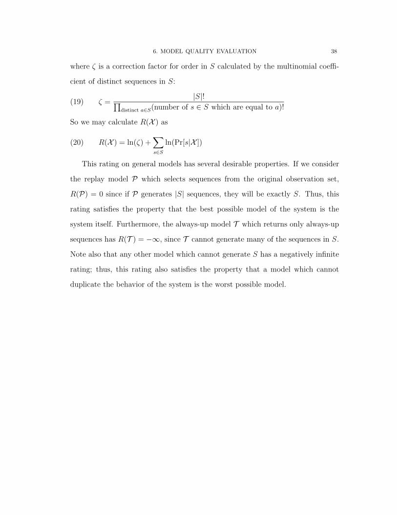
6. MODEL QUALITY EVALUATION 38
where ζ is a correction factor for order in S calculated by the multinomial coeffi-
cient of distinct sequences in S:
(19) ζ =|S|!∏
distinct a∈S(number of s ∈ S which are equal to a)!
So we may calculate R(X ) as
(20) R(X ) = ln(ζ) +∑s∈S
ln(Pr[s|X ])
This rating on general models has several desirable properties. If we consider
the replay model P which selects sequences from the original observation set,
R(P) = 0 since if P generates |S| sequences, they will be exactly S. Thus, this
rating satisfies the property that the best possible model of the system is the
system itself. Furthermore, the always-up model T which returns only always-up
sequences has R(T ) = −∞, since T cannot generate many of the sequences in S.
Note also that any other model which cannot generate S has a negatively infinite
rating; thus, this rating also satisfies the property that a model which cannot
duplicate the behavior of the system is the worst possible model.
CHAPTER 7
Results
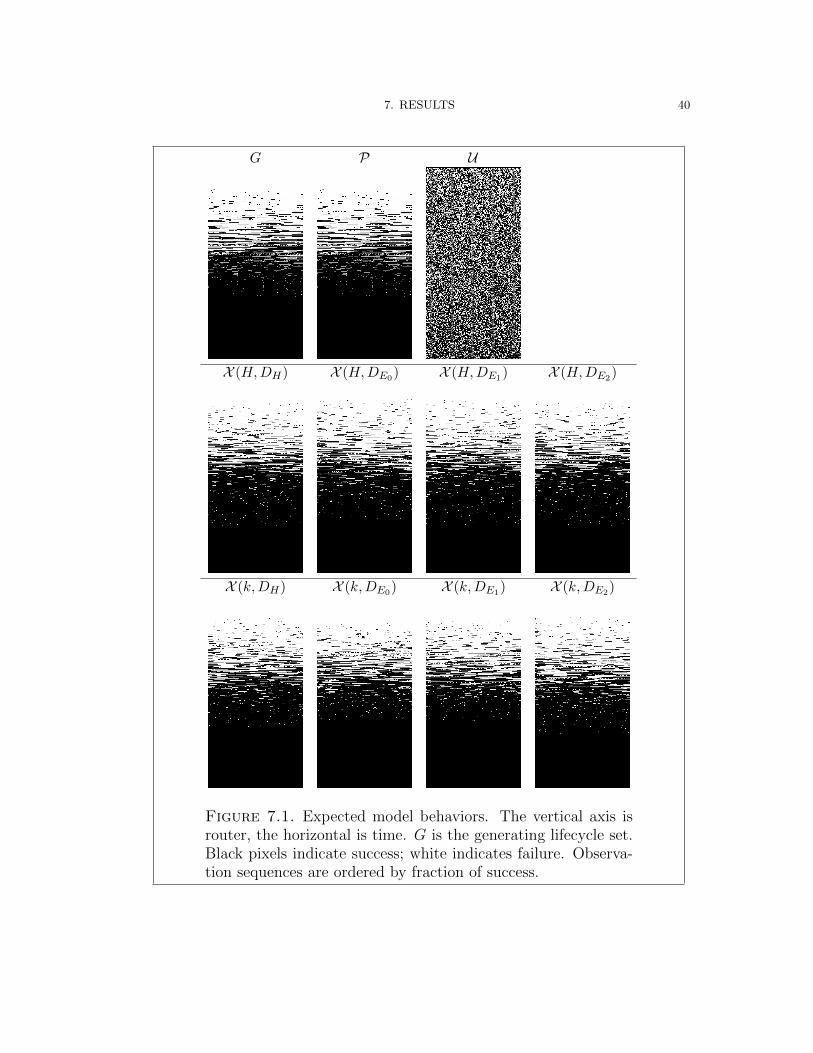
We generate models from a set G of 100 observations from each router gathered
from the Tor network from 17:18 UTC on March 23, 2011 to 11:27 UTC on March
25, 2011. These lifecycles were clustered with hierarchical and k-means clustering
according to Hamming distance and each of the three edit distance variants into
41 clusters1, and HMMs with up to 10 states were generated from each of these
clusters; the average was approximately eight states. Given clustering algorithm
c according to distance metric d, we call the resulting model X (c, d).
For comparison, we also consider the simple binomial model U which generates
sequences according to a binomail probability distribution given by the fraction
of observations in G which indicate success or failure. Of the 344500 total obser-
vations in G, 209644 were successful; thus, U at any given observation succeeds
with probability 0.6085; otherwise it fails.
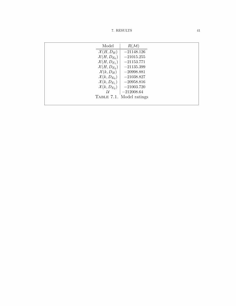
We rate each of these models against G. The ratings of each X (c, d) and U
are listed in Table 7.1. Typical model behaviors, along with G, are plotted in
Figure 7.1.
1The cluster count was selected by a rule-of-thumb calculation of√n/2 clusters from a set of n
elements.
39
7. RESULTS 40
G P U
X (H,DH) X (H,DE0) X (H,DE1) X (H,DE2)
X (k,DH) X (k,DE0) X (k,DE1) X (k,DE2)
Figure 7.1. Expected model behaviors. The vertical axis isrouter, the horizontal is time. G is the generating lifecycle set.Black pixels indicate success; white indicates failure. Observa-tion sequences are ordered by fraction of success.
7. RESULTS 41
Model R(M)
X (H,DH) −21148.126X (H,DE0) −21015.255X (H,DE1) −21153.771X (H,DE2) −21135.399X (k,DH) −20998.881X (k,DE0) −21038.827X (k,DE1) −20958.816X (k,DE2) −21003.720U −212008.64
Table 7.1. Model ratings
CHAPTER 8
Conclusion
This thesis presents a model of circuit creation in Tor which uses HMMs to
simulate router behavior. Our model simulates the behavior of Tor significantly
more accurately than the example more simplistic binomial probability model,
which is typical of models used to examine proposed attacks. This provides a
solid simulation basis for attacks which depend on the circuit creation behavior
of Tor, and upon which more detailed simulations (e.g., of latency) may be built.
Further research in some areas is needed. We have proposed and used the
probability rating to validate our model, but this is not a universally applicable
criterion, and may not always be feasible to calculate. Demonstrably applicable
validation criteria is a virtually unexplored field, and one which would be broadly
valuable.
We would like to evaluate our model against the continued behavior of Tor, by
producing an independent observation set against which to rate our model. Addi-
tionally, we would like to examine in more detail the effects of varying parameters
such as the duration of our generating observations, the number of clusters gen-
erated, or the number of states we allow in our model.
Our model was built a number of times with a small collection of clustering
algorithms and distance metrics. The behavior was similar, but not identical,
over these; examination of additional clustering algorithms and distance metrics
could be used to refine the model’s behavior. In particular, we believe that some
information-theoretic distance metrics such as mutual information could yield
42

8. CONCLUSION 43
interesting results by selecting clusters which are easy for an HMM to simulate,
rather than which demonstrate sequence similarity.
Bibliography
[1] J. Banks. Handbook of Simulation : Principles, Methodology, Advances, Applications, and
Practice. Wiley, 1998.
[2] L. E. Baum, T. Petrie, G. Soules, and N. Weiss. A maximization technique occurring in the
statistical analysis of probabilistic functions of Markov chains. The Annals of Mathematical
Statistics, 41(1):164–171, 1970.
[3] N. Borisov, G. Danezis, P. Mittal, and P. Tabriz. Denial of service or denial of security? In
Proceedings of the 14th ACM conference on Computer and communications security, CCS
’07, pages 92–102, New York, NY, USA, 2007. ACM.
[4] D. Chaum. Untraceable electronic mail, return addresses, and digital pseudonyms. Com-
munications of the ACM, 24(2):84–90, February 1981.
[5] G. Danezis. Statistical disclosure attacks: Traffic confirmation in open environments. In
Proceedings of Security and Privacy in the Age of Uncertainty (SEC2003), pages 421–426.
Kluwer, 2003.
[6] G. Danezis, R. Dingledine, and N. Mathewson. Mixminion: Design of a Type III Anonymous
Remailer Protocol. In Proceedings of the 2003 IEEE Symposium on Security and Privacy,
pages 2–15, May 2003.
[7] N. Danner, S. Defabbia-Kane, D. Krizanc, and M. Liberatore. Detecting denial of service
attacks in Tor. Unpublished version of Danner et. al., 2009.
[8] N. Danner, D. Krizanc, and M. Liberatore. Detecting denial of service attacks in Tor. In
R. Dingledine and P. Golle, editors, Financial Cryptography and Data Security, volume
5628 of Lecture Notes in Computer Science, pages 273–284. Springer Berlin/Heidelberg,
2009.
[9] R. Dingledine, N. Mathewson, and P. Syverson. Tor: The second-generation onion router.
In Proceedings of the 13th USENIX Security Symposium, August 2004.
44
BIBLIOGRAPHY 45
[10] R. W. Hamming. Error detecting and error correcting codes. Bell System Technical Journal,
29(2):147–160, April 1950.
[11] B. M. Leiner, V. G. Cerf, D. D. Clark, R. E. Kahn, L. Kleinrock, D. C. Lynch, J. Pos-
tel, L. G. Roberts, and S. Wolff. A brief history of the Internet. SIGCOMM Computer
Communications Review, 39(5):22–31, October 2009.
[12] V. I. Levenshtein. Binary codes capable of correcting deletions, insertions and reversals.
Soviet Physics Doklady, 10:707, February 1966.
[13] B. N. Levine, M. K. Reiter, C. Wang, and M. Wright. Timing attacks in low-latency mix
systems. In A. Juels, editor, Financial Cryptography, volume 3110 of Lecture Notes in
Computer Science, pages 251–265. Springer Berlin / Heidelberg, 2004.
[14] F. Liu, M. Yang, and Z. Wang. Study on simulation credibility metrics. In WSC ’05:
Proceedings of the 37th Winter Simulation Conference, pages 2554–2560, 2005.
[15] N. Mathewson and R. Dingledine. Practical traffic analysis: Extending and resisting statis-
tical disclosure. In Proceedings of Privacy Enhancing Technologies workshop (PET 2004),
volume 3424 of LNCS, pages 17–34, May 2004.
[16] S. J. Murdoch and P. Zielinski. Sampled traffic analysis by internet-exchange-level adver-
saries. In Proceedings of the 7th international conference on Privacy enhancing technologies,
PET’07, pages 167–183, Berlin, Heidelberg, 2007. Springer-Verlag.
[17] L. R. Rabiner. A tutorial on hidden Markov models and selected applications in speech
recognition. In Proceedings of the IEEE, volume 77, pages 257–286, February 1989.
[18] A. Serjantov and S. Murdoch. Message splitting against the partial adversary. In G. Danezis
and D. Martin, editors, Privacy Enhancing Technologies, volume 3856 of Lecture Notes in
Computer Science, pages 26–39. Springer Berlin / Heidelberg, 2006.
[19] R. Xu and D. Wunsch. Survey of clustering algorithms. IEEE Transactions on Neural
Networks, 16(3):645–678, May 2005.
![Tor's Been KIST: A Case Study of Transitioning Tor ... uses the circuit scheduling algorithm of Tang and Goldberg [18] to determine circuit priority. Their algorithm is based on an](https://img.pdfslide.us/doc/110x75/5b1e61b57f8b9a901f8b8f9b/tors-been-kist-a-case-study-of-transitioning-tor-uses-the-circuit-scheduling.jpg)