Embed Size (px)
Citation preview
A Simulation-based Approach to Dynamic Pricing
Joan MorrisSc.B. Applied MathematicsBrown UniversityMay 1995
Submitted to theProgram in Media Arts & Sciences,School of Architecture and Planning,In Partial Fulfillment of the Requirements for the Degree ofMaster of Science in Media Arts & ScienceAt theMassachusetts Institute of Technology
May, 2001
@ Massachusetts Institute of Technology, 2001.All rights reserved.
AuthorJoan Morris
Program in Media Arts & Sciences \0
May 11, 2001
Certified byPattie Maes
Associate Professor of Media Arts & SciencesMIT Media Laboratory
Accepted byStephen Benton
Chair, Departmental Committee on Graduate StudiesProgram in Media Arts & Sciences
MASSACHUSETTS INSTITUTEOF TECHNOLOGY
JUN 13 2001
LIBRARIES POT

MITLibrariesDocument Services
Room 14-055177 Massachusetts AvenueCambridge, MA 02139Ph: 617.253.5668 Fax: 617.253.1690Email: [email protected]://Iibraries.mit.edu/docs
DISCLAIMER OF QUALITY
Due to the condition of the original material, there are unavoidableflaws in this reproduction. We have made every effort possible toprovide you with the best copy available. If you are dissatisfied withthis product and find it unusable, please contact Document Services assoon as possible.
Thank you.
The scanned Archival thesis contains grayscaleimages only. This is the best copy available.

A Simulation-based Approach to Dynamic Pricing
Joan MorrisSc.B. Applied MathematicsBrown UniversityMay 1995
Submitted to theProgram in Media Arts & Sciences,School of Architecture and Planning,In Partial Fulfillment of the Requirements for the Degree ofMaster of Science in Media Arts & ScienceAt theMassachusetts Institute of Technology
May, 2001
Abstract
By employing dynamic pricing, the act of changing prices over time within amarketplace, sellers have the potential to increase their revenue by selling goods tobuyers "at the right time, at the right price." Software agents have been used inelectronic commerce systems to assist buyers, but there is limited use of selling agents intoday's markets. As dynamic pricing systems become necessary as a competitivemaneuver and as market mechanisms become large scale and more complex, there is agrowing need for pricing agents to be used to automate dynamic pricing, whichchallenges sellers to improve their understanding of what are the best agent pricingstrategies for their marketplaces.
This thesis addresses these issues by presenting the Learning Curve Simulator, a marketsimulator designed for analyzing agent pricing strategies for a market in which a sellerhas a finite time horizon to sell its inventory. Through an analysis of several pricingstrategies using the simulator, I demonstrate how the Learning Curve Simulator can beused as a tool for understanding the relevant factors in determining an effective dynamicpricing strategy. This simulation-based approach to dynamic pricing demonstrates atechnique which can lead to the implementation of dynamic pricing strategies in real-world markets.
Thesis Supervisor: Pattie MaesTitle: Associate Professor of Media Arts & Sciences
This research was funded in part by Mastercard International, the e-markets SpecialInterest Group, and the Digital Life Consortium.

4

A Simulation-based Approach to Dynamic Pricing
Joan Morris
The following people served as readers for this thesis:
Department o
ReaderAmy Greenwald
Assistant ProfessorF Computer Science
rown y niversitv
ReaderDan Ariely
Associate ProfessorSloan School of Management & the Media Laboratory
Massachusetts Institute of Technology
I

6

Abstract
By employing dynamic pricing, the act of changing prices over time within a marketplace, sellers
have the potential to increase their revenue by selling goods to buyers "at the right time, at the
right price." Software agents have been used in electronic commerce systems to assist buyers, but
there is limited use of selling agents in today's markets. As dynamic pricing systems become
necessary as a competitive maneuver and as market mechanisms become large scale and more
complex, there is a growing need for pricing agents to be used to automate dynamic pricing,
which challenges sellers to improve their understanding of what are the best agent pricing
strategies for their marketplaces.
This thesis addresses these issues by presenting the Learning Curve Simulator, a market
simulator designed for analyzing agent pricing strategies for a market in which a seller has a
finite time horizon to sell its inventory. Through an analysis of several pricing strategies using
the simulator, I demonstrate how the Learning Curve Simulator can be used as a tool for
understanding the relevant factors in determining an effective dynamic pricing strategy. This
simulation-based approach to dynamic pricing demonstrates a technique which can lead to the
implementation of dynamic pricing strategies in real-world markets.

8
Contents
1 INTROD U CTION .............................................................................................. 13
1.1 Finite M arkets ...................................................................................... 14
1.2 The Ballpark Exam ple............................................................................ 15Using the Simulator.............................................................................. 16Exploring M arket Scenarios................................................................... 16
1.3 Overview ................................................................................................ 19
2 E-M ARKETS & D YNAM IC PRICIN G ............................................................ 21
2.1 Today's Exam ple: Revenue M anagem ent.............................................. 22
2.2 Buyers in Electronic M arkets................................................................ 23
2.3 Theoretical Studies................................................................................ 24
2.4 Sim ulation-based Approach .................................................................. 25
2.5 M y Approach......................................................................................... 26
3 THE
3.1
3.2
3.3
LEA RN IN G CURVE SIM U LA TO R ........................................................... 29
Sim ulator Interaction D esign ................................................................ 29The Sim ulation Cycle ........................................................................... 29M arket Scenario ..................................................................................... 30Buyer Behavior...................................................................................... 32Seller Strategies..................................................................................... 33Sim ulator Output ................................................................................... 37
Sim ulator Code D esign ......................................................................... 39
Sim ulator Strategies .............................................................................. 42Goal-D irected........................................................................................ 42D erivative-Following ........................................................................... 43
4 STRATEGY ANALYSIS .................................................................................. 45
4.1 Analysis Process..................................................................................... 45
4.2 Monopoly: One Seller in the Market..................................................... 47
4.3 Competition: Two Sellers in the Market ................................................ 52
4.3.1 Further Market Variation: Buyer Segmentation..................................... 57
4.4 Strategy Analysis Conclusions.............................................................. 61
5 U SA GE A N A LY SIS......................................................................................... 65
5.1 Sim ulator as an Interface....................................................................... 65
5.2 Sim ulator as a Tool ................................................................................ 66
6 CO N CLU SIO N ................................................................................................ 69
6.1 Further Strategy D evelopm ent .............................................................. 69
6.2 M ore Realistic Buyer Behavior.............................................................. 70
6.3 Buyer Response..................................................................................... 70
6.4 M arket Types.......................................................................................... 71
REFEREN CES..................................................................................................................73
10

Acknowledgements
I would like to thank, first, Pattie Maes, a great advisor and advocate during my two years at the
lab and through the Master's thesis process. Simply put, she has inspired not just my research, but
me!
Thank you to my thesis readers, Amy Greenwald and Dan Ariely, who both offered challenging
perspectives on this work. I particularly want to thank Amy for her enthusiasm for the simulator
and for the success of my research.
Thank you to all the Agents, past and present, especially Jim Youll and Sybil Shearin. It has been
great to be part of an active research community and I hope we continue to collaborate through
the years.
I'm indebted to my UROP, Kaska Dratewska, who ran countless simulation trials in the late night
hours for the sake of my paper deadlines! The simulator interface also benefited from her bug
testing and feedback.
Finally, thanks to my family and to Mike DiMicco, for your loving support and for all those
important things you've taught me over the years.

12

1 Introduction
Today, when a ballpark sells baseball tickets, the park charges the same price for the tickets
throughout the season. Yet the demand for tickets changes over time depending on the length of
time before the game, the team's success over the season, and unpredictable factors such as the
weather. In a best-case scenario, a park sells all of its seats for every game at an optimal fixed
ticket price. In a more realistic scenario, some days the park has empty seats and on other days
the park is filled with buyers willing to pay more. Nonetheless, today ballparks leave the practice
of dynamic pricing to scalpers.
Dynamic pricing, defined as the changing of prices in a marketplace, can be implemented in
several different ways. Price discrimination, or personalized pricing, is an intriguing area of
dynamic pricing in which sellers charge different segments of customers different prices. While
this area is rich with potential, it also has greater risks of customer rejection, as exhibited when
Amazon.com experimented with charging customers different prices [2]. In contrast to this
approach to dynamic pricing, this body of work focuses on the changing prices over time in a
market that makes no assumptions or attempts to segment the buyer population into sub-groups.
This perspective on dynamic pricing focuses on how a seller can take advantage of the
fluctuations in cumulative buyer demand over time, taking into account a finite time horizon. In
this thesis, I refer to this type of changing of prices over time as dynamic pricing.
Cost is perhaps the greatest factor precluding the widespread use of dynamic pricing by ballparks
and other markets. In traditional markets, it is expensive to continuously re-price goods, but in
digital markets, the costs associated with making frequent, instantaneous price changes are
greatly diminished [25]. Moreover, in markets under a finite time horizon, such as ballparks,
theaters, seasonal retail stores, rental cars, and other perishable good markets, a clear benefit to

changing prices over time is that one can ensure all inventory is sold. Thus, it seems likely that in
the near future, dynamic pricing will become a common competitive maneuver, particularly in
markets under a finite time horizon.
A remaining obstacle that hinders widespread dynamic pricing is the difficulty in understanding
the complexities price changes introduce into a market. Now that sellers can easily implement
frequent adjustments to price, how should they do so? What are the most effective dynamic
pricing strategies, and how do they behave in specific markets? I propose that sellers should
analyze dynamic pricing algorithms using a market simulator that is capable of simulating many
different market scenarios with realistic models of buyer behavior. Using a market simulator, a
seller could model its market's characteristics and the behavior of its customers, to develop a
pricing strategy that could capture more profit than fixed-price policies.
To illustrate my proposed approach, I present in this thesis the Learning Curve Simulator, a
platform for running dynamic pricing algorithms in simulated markets. Through an analysis of
different pricing strategies under varying market conditions, I demonstrate how, by observing
market conditions, a seller can take advantage of fluctuations in buyer demand to earn more
revenue and sell more inventory.
1.1 Finite Markets
My investigation of dynamic pricing strategies focuses on an extremely common market type,
which I call a finite market -- a market with a finite time horizon, seller inventory, and buyer
population. Examples of finite markets include event tickets, airlines, hotels, perishable goods,
and seasonal retail.
Facing the need to liquidate inventory, sellers in finite markets often choose to sell remaining
inventory in a side market where it is referred to as "distressed inventory." Examples of such
markets on-line are LastMinuteTravel.com [24] for airline tickets and FairMarket's
AutoMarkdown [19] for retail. AutoMarkdown runs as a multi-unit Dutch auction [19] in which
items are initially offered at a high price and then offered at a progressively lower price, down to
a specified minimum, or until all inventory is sold. While AutoMarkdown's pricing strategy is
basic and does not respond to demand in the marketplace, it is a good example of how dynamic
pricing can achieve a finite market's seller's goal of selling all of the inventory.
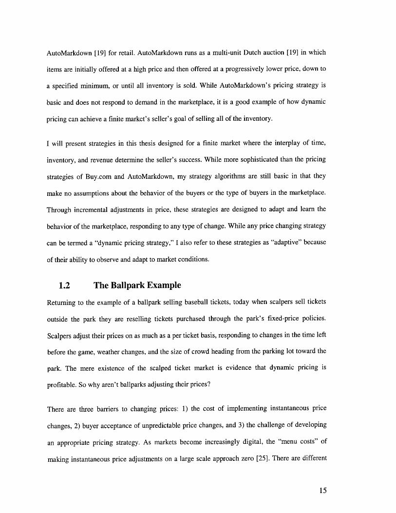
I will present strategies in this thesis designed for a finite market where the interplay of time,
inventory, and revenue determine the seller's success. While more sophisticated than the pricing
strategies of Buy.com and AutoMarkdown, my strategy algorithms are still basic in that they
make no assumptions about the behavior of the buyers or the type of buyers in the marketplace.
Through incremental adjustments in price, these strategies are designed to adapt and learn the
behavior of the marketplace, responding to any type of change. While any price changing strategy
can be termed a "dynamic pricing strategy," I also refer to these strategies as "adaptive" because
of their ability to observe and adapt to market conditions.
1.2 The Ballpark Example
Returning to the example of a ballpark selling baseball tickets, today when scalpers sell tickets
outside the park they are reselling tickets purchased through the park's fixed-price policies.
Scalpers adjust their prices on as much as a per ticket basis, responding to changes in the time left
before the game, weather changes, and the size of crowd heading from the parking lot toward the
park. The mere existence of the scalped ticket market is evidence that dynamic pricing is
profitable. So why aren't ballparks adjusting their prices?
There are three barriers to changing prices: 1) the cost of implementing instantaneous price
changes, 2) buyer acceptance of unpredictable price changes, and 3) the challenge of developing
an appropriate pricing strategy. As markets become increasingly digital, the "menu costs" of
making instantaneous price adjustments on a large scale approach zero [25]. There are different

ways of managing buyer expectations when implementing dynamic pricing, and these issues will
be addressed in this thesis's Conclusion. To address the third challenge, of making instantaneous
strategic changes in price, I propose a ballpark, or similar seller, use a market simulator to model
their market and analyze which pricing strategy is best for their marketplace. And in the next
pages, I demonstrate how this approach would work.
Using the Simulator
A ballpark stands to earn more revenue if it can change its prices in such a way as to take
advantage of the fluctuations in buyer demand over time. To understand how this can be done, a
ballpark would use the Learning Curve Simulator to model its market and the behavior of its
buyers. The market conditions: the number of potential game attendees, ticket sellers, seats in the
park, and days in the market, define the 'finite' nature of the ballpark's market. The behavior of
the buyers is described in the Learning Curve Simulator in terms of how the buyer population
varies on an individual day and over time. Over time, the amount buyers are willing to pay,
referred to as their valuation, can fluctuate. The user can choose different shaped curves to
express different valuation over time changes. On a single day, the dispersion between the
individual buyers is expressed through several variables, including a variance and distribution of
the buyers' demand (buyers vs. price curve). The ballpark sets up these parameters in the
simulator to begin an analysis of dynamic pricing in its market.
Exploring Market Scenarios
After setting up the basic ballpark market parameters, the ballpark can compare different
combinations of strategies in the simulator. Choosing to compare one fixed price seller against
one of the simulator's adaptive pricing strategies allows the ballpark to analyze today's situation
where the ballpark offers a fixed price and scalpers adjust their ticket prices over time.
The way the ticket buyers' valuation changes over time is hard to predict when it depends on

external market conditions such as weather and the success of the baseball team. Thus it is
important to test the success of any pricing strategy under a variety of unpredicted valuation
fluctuations. To do this, the ballpark would run multiple simulation trials under different
valuation/time curve shapes, for example decreasing, increasing, mid-dipping, or mid-peaking
valuation over time.
The charts in Figure 2.4 present the pricing, revenue and sales results of four different trials, as
they would be presented in the simulator's interface. Under the first three trials, the adaptive
pricing strategy earns more revenue and sells all the ballpark tickets in the park. The fixed-price
strategy sells tickets at a price point that could not sell all the seats in the park. In trial four, the
fixed price was at a level that did sell all the tickets and the two strategies performed equally well.
After running a batch of such simulations, a ballpark could adjust different market parameters and
continue to run exploratory simulations. In addition to adjusting different market parameters, the
ballpark could try different dynamic pricing strategies and fine-tune their behaviors. By also
adjusting the price offered by the fixed-price seller, different fixed-prices could be found that
earned more revenue than the pricing strategies, but as the ballpark would discover, many of the
possible adjustments in market parameters, such as changing the valuation/time curves, would
reverse the fixed-price seller's success.
Through working with the simulator, the ballpark would see that using an adaptive pricing
strategy ensures a certain amount of success, regardless of the market's behavior. If a perfect
prediction of buyer valuation over time could be made, then an optimal fixed price could be
chosen, but when that optimal price cannot be chosen, an adaptive pricing strategy, demonstrates a
better performance under most conditions.
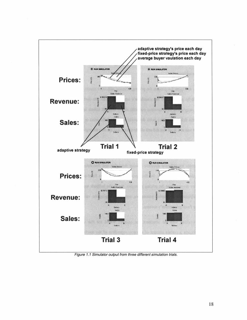
adaptive strategy's price each dayfixed-price strategy's prie, each dayaverage buyer vaulation each day
Prices:
Revenue:
Sales:
Trial 1 Trial 2adaptive strategy fixed-price strategy
.9 A6A o ^%Aen
Prices:
Revenue:
Sales:.
Trial 3 Trial 4
Figure 1.1 Simulator output from three different simulation trials.
One of the goals of this research is to develop a tool that a ballpark, or similar seller in a finite
market, could use to explore and understand the conditions for which an adaptive or other
dynamic pricing strategy works. By working with the Learning Curve Simulator, a ballpark can
model its market and test different strategies, to determine an optimal pricing strategy for its
specific market conditions. Once an optimal strategy has been determined, a ballpark could take
its algorithm and further customize it for the real-world market and eventually deploy the strategy
to perform automated price changes in the baseball ticket market.
1.3 Overview
In the following chapter, I will discuss the theoretical underpinnings for this research, with a
presentation of related work done in the area of dynamic pricing. In the following chapter, I
present the design and implementation of the Learning Curve Simulator, from the perspective of
the user-interface interaction as well as the backend code design, highlighting how aspects of the
simulator are designed to be flexible enough to facilitate future development.
The next two chapters, Strategy Analysis and Usage Analysis, I evaluate the simulator from two
perspectives: the simulator as a tool for evaluating pricing strategies and the simulator as a tool to
assist real-world sellers in understanding dynamic pricing. My analysis of pricing strategies
includes an in-depth analysis of two adaptive pricing strategies termed Goal-Directed and
Derivative-Following. These strategies are basic learning algorithms which demonstrate a high
amount of success over a fixed-pricing policy. My hope is that in addition to demonstrating the
power of a simulation-based approach to strategy analysis, these specific strategies will lay the
groundwork for designing more complex algorithms to be deployed in real-world markets. My
evaluation analysis of the simulator as a tool for real-world sellers consists of conclusions from
meetings with different sellers planning on implementing dynamic pricing. The feedback on the
simulator and information about these different sellers' markets highlights some of the challenges
in building a general simulator for multiple marketplaces.

This thesis proposes a way of approaching the problem of pricing strategy implementation. We
believe dynamic pricing is a powerful idea for increasing revenue in an electronic marketplace,
but how should a seller implement effective pricing strategies? In the business strategy magazine
Darwin Online, the difficulty and risks of dynamic pricing are summarized with a warning to
sellers: "poorly implemented pricing schemes create the potential for competitive price wars and
lowered profitability for all" [16]. The Learning Curve Simulator is designed to alleviate these
risks of dynamic pricing by providing a mechanism and approach for understanding dynamic
markets and analyzing pricing strategies.

2 E-Markets & Dynamic Pricing
Before exploring the details of the Learning Curve Simulator, it is important to understand the
state of today's electronic markets and the previous work done in the area of dynamic pricing.
Electronic markets have dramatically reduced the cost of making changes to price [25], so for the
first time sellers are able to realistically make immediate and timely adjustments to price. As
evidence of this, several on-line businesses today make automated adjustments in price, as much
as every hour.
An example of one such on-line business is Buy.com. As described by [25], Buy.com uses
software agents to search competitor's web sites for competing prices, and in response, Buy.com
lowers its price to match or beat these prices. Their simple pricing strategy is based on the
assumption that their customers are extremely price sensitive and will choose to purchase from
the seller offering the lowest price. Not surprisingly, Buy.com has managed to garner enormous
sales, but their profits are extremely low, or even negative.
The example of Buy.com highlights two things. First, automated dynamic pricing is a feasible
option for companies today. Second, an overly simplistic or incorrect model of buyer behavior
can produce undesirable results. Today's economy is ready for dynamic pricing on a more
complex scale: more complex in its understanding of buyer behavior and its pricing algorithms.
With these changes, sellers stand to increase profits through dynamic price adjustment.

2.1 Today's Example: Revenue Management
The airline industry provides a more sophisticated example of dynamic pricing in today's
economy. The airlines use the technique of revenue management to dynamically adjust prices
over time by adjusting the number of seats available in each pre-defined fare class, or booking
class [5, 21, 24]. Commercial revenue management systems forecast demand, monitor booking
activities and, in response, adjust the number of tickets available at each fare level. This method
is extremely profitable for the airlines and practiced in other industries such as hotel rooms, the
cruise industry, and rental cars. Its success is based on these industries' ability to segment their
buyers into different groups with different levels of willingness to pay. Some claim a distinct
difference between revenue management and dynamic pricing [4] because of this buyer
segmentation, which is not a necessary aspect of dynamic pricing. My investigation of dynamic
pricing does not focus on buyer segmentation, or price discrimination, but the airline industry's
adjustment of prices over time still demonstrates the potential of earning more revenue by
charging "the right customer, the right price, at the right time."
The techniques of revenue management require sellers to make sophisticated assumptions and
predictions about the behavior of the marketplace. This limitation was addressed by Gallego &
van Ryzin [12] in their discussion of the need to merge the ideas of revenue management with
dynamic adjustment of prices, where pricing is determined in response to consumer demand. As
the revenue management industry exists today, the prices in each fare class are fixed, yet these
price levels influence the market. For example, when the lowest fare class is sold out, the demand
for the second-lowest fare class increases. In their work, Gallego & van Ryzin propose a model
for blending revenue management, or dynamic programming, with price adjustments based on
observed demand, and suggest that this model of price adjustment be applied to new industries,
such as the fashion and retail industries.
2.2 Buyers in Electronic Markets
While methods exist for using historical data to predict market behavior [21], the potential
problem with using previous data to make assumptions about the future, is the risk of being
wrong. For example, marketers have made assumption about the behavior of buyers on-line
which have been shown to be incorrect.
There is increasing evidence that while the search costs of finding products on the Internet are
lower than in the off-line world, there is not a corresponding increase in buyers' sensitivity to
prices [10]. Even with tools such as shopbots performing the task of locating goods and
comparing prices, buyers seldom purchase from the lowest priced seller, revealing that they have
a more complex utility function for that good or vendor. Additionally, when buyers have more
information about a product, as they can more easily find in an electronic market, they become
even less price sensitive [8]. Another interesting observation of on-line markets is that price
dispersion, traditionally thought to be caused by high search costs, can still be high in an
environment of low search costs, presumably when buyers have preferences for certain products
and sellers [7].
The new purchasing environment created by electronic markets has revealed new and somewhat
unpredicted buyer behavior. Initial attempts at providing buyers with shopping assistance
(shopbots) and initial use of software agents to adjust prices (Buy.com) both assumed that buyers
were extremely price sensitive. Because this has been shown to not be the case, there is a need for
more complex tools for buyers [15, 22] and for sellers. I propose the Learning Curve Simulator as
a tool that will allow sellers to deploy dynamic pricing in an electronic marketplace filled with
complex buyers.

2.3 Theoretical Studies
Earlier work of Gallego & van Ryzin [13] built a theoretical model for calculating optimal prices
for finite markets. This model addresses the challenge of dynamic pricing in finite markets, but
from a theoretical standpoint. They examine a deterministic version of the problem of pricing
under finite time horizons by making the assumption that consumers' demand curves do not
change over time. Under these conditions, they conclude that the optimal pricing strategy is
"jittery" and requires constant price adjustments, something they considered to be infeasible at
their date of publication (1994). They concluded that a fixed-price strategy works "surprisingly
well" when the demand curve is known. A "nearly optimal solution" is to have a fixed set of
tiered prices that the seller oscillates between, and this is proposed as a more feasible solution
than the optimal solution (of continual, incremental price adjustment).
These results can be easily duplicated in the Learning Curve Simulator. When the demand curve
is known, a best fixed price can be selected to nearly optimize revenue, even under cases of
changing demand curves over time. But what my analysis of pricing strategies emphasizes is that
one cannot assume perfect knowledge of the demand curve, something to which Gallego and van
Ryzin concede is more realistic.
In a recent analysis of the automotive industry [4], Biller et al. designed a theoretical model for
applying dynamic pricing to a marketplace with unknown changing demand levels. They
demonstrate that under fluctuating demand there is always an optimal dynamic pricing strategy
which is successful over a fixed-price strategy. The degree of success of the strategy increases
depending on the amount of variance among the buyer population and the number of times the
seller adjusts prices. Their model [9], focuses on a market with no limits on production, so not
"finite," but these results are similar to the results we have found in the simulator.
2.4 Simulation-based Approach
While a theoretical approach to agent pricing strategies could be taken, a theory-based solution is
often difficult to apply to a real-world marketplace because of the overly simplifying assumptions
that typically need to be made in developing a theoretical model. Simulated marketplaces are able
to model more diverse and complex scenarios, rather than the general case. By producing
tangible, numerical results, the Learning Curve Simulator can be used as a tool for understanding
real-world scenarios.
Researchers at IBM have made significant headway [14, 17, 18] in examining the results of buyer
and seller agent-driven markets, focusing on markets of information goods. Their analysis of
agent-driven markets highlights through simulation some of the potential pitfalls of automated
dynamic pricing, such as price wars. In their analysis, they introduced four different agent pricing
strategies: game theoretic, derivative following, myopically optimal (dynamic programming), and
Q-learning (reinforcement learning). Their game theoretic strategy was used as a benchmark,
under the assumption of rational behavior of all buyers and sellers. The complexity of buyer
behavior in the Learning Curve Simulator prevents the ability to make this assumption of
rationality in strategy analysis. Their specific algorithm for the derivative following strategy was
adapted for finite markets and will be analyzed in the Learning Curve Simulator. Their work has
provided a strong background for this investigation of successful strategy development.
Brooks et al. [6] also performed analysis of pricing agents in a simulated market environment and
discussed the trade-offs between "exploitation" and "exploration" pricing techniques on the part
of the seller. They conclude that when a pricing agent is interested in maximizing revenue over a
longer period than the immediate purchase period, a simple learning algorithm works best for
markets with high levels of uncertainty. While Brooks examines markets of information goods
with no constraints on time or inventory, their use of a simulator to demonstrate the strength of
different strategies provides a useful guideline for our analysis.

2.5 My Approach
The McKinsey Quarterly [2], a quarterly publication on business strategy, recommends sellers
pursue dynamic pricing on-line and start by running different pricing experiments. They state that
by making small adjustments in price, sellers can discover the demand levels of their buyers.
Despite the abundance of the theoretical studies and optimal pricing strategy conclusions found in
the literature, for the real-world seller, making predictions about buyer demand and implementing
this as a strategy is far from straightforward, and yet McKinsey's overly simplistic
recommendation addresses this difficulty. I propose that the Learning Curve Simulator be a
model for a practical tool sellers can use to study different pricing strategies, so their exploratory
pricing schemes can be more strategic and informed, both by the literature and through first hand
experience with a simulated market environment.
As discussed in this chapter, the use of a simulator is a powerful and practical approach to
dynamic pricing strategy analysis, and can serve as a platform for modeling the complex
behaviors of buyers on-line.
The Learning Curve Simulator, as a tool for sellers, addresses the complexities of on-line buyer
behavior by providing a rich set of behavior parameters. First, the buyer population in the
simulator can be divided into two groups, who each behave according to their own sets of
behavior parameters. This allows for the expression of different types of buyer populations within
the simulator. To express the dispersion within each group of buyers, the simulator allows for a
variance to be indicated for a chosen buyer/price distribution curve. Additionally, price sensitivity
is expressed with a selection of the percentage of buyers are comparison shoppers. Preference for
a particular type of good or seller is expressed in an option to select a seller as "preferred."
Although not a complete or exact model of real-world markets, especially because individual
markets contain their own idiosyncrasies, this is a more expressive set of variables than any
previous set of simulation-based work for dynamic pricing analysis.

In contrast to the strategies developed by other researchers, the strategies implemented in the
Learning Curve Simulator are based on machine learning concepts, and thus referred to as
'adaptive.' Each of the strategies makes no assumptions about the rationality of market players,
but instead makes basic observations and adjustments in price each day.
The following chapter presents the Learning Curve Simulator and two adaptive pricing strategies,
the Goal-Directed and Derivative-Following strategies, which will lay the groundwork for
demonstrating the simulator's ability to serve as a practical tool for dynamic pricing strategy
development.

28

3 The Learning Curve Simulator
To present the Learning Curve Simulator, this chapter first discusses the simulator's user
interface with a description of the user interaction. Next, this chapter covers a high-level
description of the back-end code, highlighting the structure of the underlying design. Finally, the
two pricing strategies implemented in the simulator are presented, along with their pricing
calculations.
3.1 Simulator Interaction Design
The Learning Curve Simulator's graphical interface is a Java Swing application, which can run as
either a client application or a web applet. It simulates a market based on user-supplied
parameters defining a Market Scenario, Buyer Behaviors, and Seller Strategies. The Learning
Curve Simulator's interface is shown in Figures 4.1 through 4.5. This series of screens illustrates
the steps a user takes to set up a model of his/her market and run simulations. Table 4.1 outlines
the input parameters collected on each input screen, as discussed below.
Figure 4.1 shows the initial screen of the simulator. At this screen the user selects from a defined
scenario to pre-fill the following input screens, or chooses to build a custom market scenario. The
first three selections are based on the real-world markets of airline tickets, a grocer selling
produce, and a ballpark selling tickets. The remaining selections are designed to illustrate certain
strategic results.
The Simulation Cycle
Before detailing the exact simulator inputs, it is useful to first present how the simulator runs a
simulated marketplace based on the inputs. After a user has progressed through the screens in
Figures 4.2-4.5, he/she hits the "Run Simulator" button. At that moment, the simulator

sequentially runs through each "day," or time period, of the market. Each day, a random number
of buyers enter the market, based on a uniform distribution of buyer entrance over the entire
market. These buyers stay in the market until either they have purchased a good or their lifetime
has expired. On a single day, each buyer, in random sequence, searches through the available
sellers, in random sequence, and compares the seller's price with its own reservation price. If the
seller's price is less, a transaction occurs and the buyer leaves the market. If the seller's price is
more, the buyer continues looking. The day ends when each buyer has completed its search
through the sellers. At the end of the day, a new reservation price for each buyer is calculated
based on the user-provided buyer behavior parameters, and each seller updates its price based on
its chosen pricing strategy. If the seller is using a Fixed-Price strategy, there is no change to the
price. If the seller is using an adaptive pricing strategy, the seller examines different results from
the market, such as how many goods it has sold or how much revenue it has made in the previous
day and uses this information to calculate a new price. In this manner, the market progresses until
the last day, stopping only if there are no more buyers or no more goods in the market.
The speed of each simulation run depends on the number of buyers in the market who need to
search through the sellers. A simulation with 4000 buyers runs in approximately three seconds
and the same simulation with 40,000 buyers runs in approximately 30 seconds.
Market Scenario
Now that the process of providing the simulator input parameters is presented. The first series of
simulator inputs are the Market Scenario inputs, shown in Figure 4.2. The Market Scenario is
used to set the parameters of the finite market: the number of days, buyers, sellers, and goods. It
also sets the market mechanism, buyer population segmentation, the costs of the market (cost of
production and marginal cost per good), and the initial price offered by the sellers.
The number of days defines the number of periods the sellers can change their prices and the

number of instances buyers can enter the marketplace. The number of sellers in the market
determines whether or not this is a monopoly or competitive environment. The number of goods
per seller, as compared with the number of buyers, determines which parameter constrains the
market: buyers or goods. The choice of constraining parameter effects the outcome of different
strategies as will be shown in the analysis section.
The buyer population can be segmented or divided into two groups, either into a 50/50 split or a
75/25 split. By segmenting the buyers, the user then will define separate buyer behavior
parameters for each of these groups and they will be joined in one population for the market
simulation. The purpose of segmenting the population is to allow for users to express different
sub-groups within their customer population.
The sellers' costs are defined as the cost of production and the marginal cost per good. Many
finite markets, such as a ballpark, have a marginal cost of zero per good, so the major cost of the
market is the initial cost of production. Although an overly simplistic assumption, the costs for
each seller in the simulator are considered to be identical. Because it is assumed that margin costs
are low (i.e. negligible) and because there is no distinction made between each seller's costs, the
results of the simulation are reported in terms of revenue (price * units sold), not profit (revenue -
costs).
The "initial price" input value is the price offered by each of the sellers on the first day of the
market. This value can be adjusted on a per seller basis on the Seller Strategies screen.
When setting the market mechanism, the user chooses between Posted-Price and First-Priced
Auction. A Posted-Price market is the typical market consumers face today in which sellers
publicly post prices and buyers view the prices and choose to purchase for that price, or not. The
other choice for market mechanism is a very basic auction, termed a First-Price Auction. In this
auction, there is one bidder per seller at each instance. When a buyer places a bid equal to its

reservation price, it is compared to the seller's reserve price and if it is higher, then the buyer pays
the bid price for the good. There is no competition between the bidders and the bidders do not
know the sellers' prices in the marketplace. The purpose of building this auction mechanism was
to test different strategies designed for an auction scenario.
Buyer Behavior
After defining the Market Scenario, the user then defines the behavior of the buyers in the market,
both in terms of their behavior on a per day basis and their behavior over time. These parameters
are shown in the screenshots in Figures 3.3 and 3.4.
The behavior of the buyers on a single day of the market is defined in several ways. First, the
buyer population can be segmented into two groups, defined by the Market Scenario on the
previous screen, in a ratio of either 50/50 or 75/25. When the buyer population is segmented,
there are two tabs in the interface for these two groups, and each of the buyer parameters can be
defined for these separate groups. The results of the market simulation will present the
combination of the two buyer segments as one population.
For each buyer segment, the dispersion among the buyers' reservation prices each day is defined
by the variance and daily buyer/price distribution. The variance sets the range for the spread
along the chosen distribution curve. The distribution curves model different types of demand
curves: the common decreasing curve, an increasing curve which could apply to a luxury item
where more buyers are willing to pay more for the good, a double peaked curve which applies to
markets with two-tiers of buyers (such as leisure and business travelers), and a mid-peaking curve
which applies to a market in which there is a commonly understood average value for the item.
In addition to modeling the dispersion among buyers each day, the user has the choice of how
many buyers will be comparison shoppers. Comparison shoppers are defined as buyers who look
at the prices of each seller and buy from the seller with the highest percentage discount below

their reservation price. When a buyer is not a comparison shopper, it will check multiple sellers'
prices only until a match and will then immediately purchase.
The final parameter determining the daily behavior of buyers is the designation of certain sellers
in the market as "preferred." A preference for a seller can express real-world differentiation
among products and sellers, due to higher quality, better product features, and brand loyalty.
When a seller is selected as preferred, buyers are willing to pay 20% more for that seller's
products. While this percentage mark-up is configurable in the back-end of the simulator, it was
designed in this basic form to simplify the interaction with the simulator.
The behavior of the buyers over time is defined by four variables: the lifetime, the minimum and
maximum prices, and the valuation curve, each shown in the bottom half of the Buyer Behavior
screens, in Figures 3.3 and 3.4. The lifetime parameter indicates how "patient" the buyers are:
how many days they are willing to wait in the market, continuously looking for the right price. If
the buyer is still looking at the end of its lifetime, it leaves the market without purchasing. The
valuation curve choice determines how the buyers' average reservation prices, or valuation,
changes over time, by either a flat, decreasing, increasing, mid-dipping, or mid-peaking curve.
The minimum and maximum prices define the minimum and maximum values on this
valuation/time curve. The buyers' valuation on a single day is a significant factor in how many
sales a seller makes, and the more successful sellers are the ones that can effectively follow the
changes in the buyers' valuation over time.
Seller Strategies
The final step to setting up the market is to specify which pricing strategy each seller uses, shown
in the left pane of the final screenshot, Figure 3.5. The simulator is designed to allow multiple
strategies to work within the same market, so a user can compare how a strategy performs
compared with other strategies in the marketplace. For simplicity of comparison, a maximum of

four strategies can be presented at one time in the simulator, and only three are shown in Figure
4.5. The three strategies available are Fixed-Price, Goal-Directed, and Derivative-Following.
Each of these strategies are discussed and evaluated in the Strategy Analysis chapter.
The user can adjust each strategy by changing the initial price offered by the seller and by
choosing to limit the number of goods sold in a single day for each seller. Changing the initial
price effects the first day of sales, and of course, every day after in the case of a Fixed-Price
strategy. Some of the strategies use this initial price in the pricing calculation, so this initial price
also effects the behavior of these strategies over time. Sales can be limited each day to represent
actual market limitations to selling an entire inventory in a single day. When the user chooses to
limit the sales, that seller can only sell three times the ratio of goods to days. In practice, this
constricts the behavior of the sellers, producing less drastic changes in prices because there are
less drastic discrepancies in sales between days.
L..i-g x,"Fite
Welcome
Choose a pre-defined market or define a custom marketscenario:
() Airline Scenario (IC-Al)
O Grocer Scenario (EC'01)
O Ballpark selling tickets
O Derivative Following wins under large buyer population
O Derivative Following wins under comparison shoppers
C Goal Directed wins with a higher initial price
O Goal Directed wins with increasing demand
O Goal Directed-Quantity wins with a first-price auction
OD Custom market scenario...
) NEXT
Learning Curve
Figure 3.1: Learning Curve Simulator - Choose from a pre-defined scenario

Market
Nurmber of Days: 60
Number of Buyers: 5000
Market Mecharm Postedr-i
Segment Buyer Population? Yes,50%-50%
Sellers
Number of Sellers 5
Number of Goods per Seller: 1000
Fixed Cost F$) 5000
Marginal Cost per Good ($): 10
initial Price
NEXT
SIMULATOR OUTPUTS
Figure 3.2: Learning Curve Simulator - Defining a market scenario
I earnnmo (ur ve S)imulator PIER E3
Buyer Behavior Each Day
Price Variance Each Day (+/-$) 25
Price Distribution (Buyers/Price): 0 012 0 - @
% Comparison Shoppers:0 25 50 75 100
Preference for Certain Sellers:
_j SellerA 0 Seller B E Seller C
El Seller D 0 Seller E
Buyer Behavior Over Time -
Buyers' Lifetime in Market:
Buyers' Min Price ($): 100 Buyers' Max Price($): 300
Change in Buyers'Prices overTime:
SIMULATOR OUTPUTS
Figure 3.3: Learning Curve Simulator - Defining the behavior of buyer population segment A

F. .. ._3i~~~ eanrgCreSmltru]1
SIMULATOR OUTPUTS
Figure 3.4: Learning Curve Simulator - Defining the behavior of buyer population segment B
:rt eaining Curve Simulator P~i r
SelrStrategIes,
Strategies Sellers
A B C D E
Fixed Price 0 0 0 0 @Derivative Following a 0 @ @ 0Goal Directed @ 0 0 0Goal Directed Quantity 0 0 0 0 0
Limit Goods Ea Day? [ Fd F ji P:lInitial Offer Price ($) F0011 001130011 F12
o RUN SIMULATOR
o RUN 100 SIMULATIONS
U Average Buyer U Seller AU Seller B U Seller C2 Seller D 0 Seller E
Figure 3.5: Leaming Curve Simulator - Choosing the pricing strategies and viewing simulator results

Simulator Inputs: DescriptionMarket Scenario:Number of Days Number of periods in the market. Each seller can change its price at the end of a day.Number of Buyers The size of the buyer population over the entire market.Market Mechanism Posted-Price or First-Price Auction.Buyer Segmentation The buyer population can optionally be divided into two groups, either in a 50-50 or 75-25 ratio.Number of Sellers Number of sellers.Number of Goods Initial inventory for each seller.Fixed Cost Cost of producing the inventoryMarginal Cost per Good The additional cost of selling each good. This is often zero in a finite markets.Initial Price Offered The initial price all the sellers will offer in the market. This parameter can be adjusted on a per
seller basis on the Seller Strategies screen.Buyer Behavior:
Daily Price Distribution The demand distribution of buyers on a single day. Available choices are normal distribution,positive slope, negative slope, or segmented into a high and low grouping.
Price Variance Per Day The buyers' reservation prices vary ± the variance in a single day. The variance determines therange for the daily price distribution.
Percentage Comparison The percentage of the buyer population (0-100%) who compare each seller's offer price andShoppers purchase from the seller with the greatest % discount below its reservation price for that seller.Preference for Certain Sellers The entire buyer population can have a preference for one or more of the sellers, which is
represented by a higher reservation price for that individual seller. This is a method forexpressing product and seller differentiation.
Lifetime Number of days a single buyer will be in market, actively looking for seller. Regardless oflifetime, once a buyer purchases, it leaves the market.
Buyer Valuation over Time Over the course of the market, the buyers' demand curve will change, and the valuation/timecurve expresses how the demand will change over time. The shape of the curve can be either flat,increasing, decreasing, mid-peaking, or mid-dipping over time.
Minimum/Maximum Buyer The range of prices for the buyer valuation curve. These values are the minimum and maximumPrices over Time reservation prices over the market.Seller Behavior:Seller Strategies The different pricing strategies sellers use in the market, either Goal-Directed or Derivative-
Following. .Initial Prices The different prices sellers offer on the first day of the market, before adjusting price through the
chosen strategy.Available Inventory per Day Amount of inventory a seller can sell in one day. This can be limited to represent shelving costs
and to prevent 100% inventory sell-off in a single day.Table 3.1: Leaming Curve Simulator Inputs
Simulator Output
After the simulator runs, the results are presented in the right pane of the interface, as shown in
Figure 3.5. These results summarize the market in terms of pricing, revenue, and sales. Additional
output detailing each day and each transaction is also saved to a tabbed-delimited file on the
user's machine. If the user had clicked 'Run 100 Simulations,' after 100 identical simulations ran,
an output file would be created for each simulation, and a summary file would be generated that
reported the final revenue and sales of each seller per simulation.
Returning to the visual output presented in the interface, the top chart in Figure 3.5 shows the
pricing behavior of each seller on each day in relation to the average reservation price of the
buyers. The next two charts report the revenues and sales of each seller. Revenue is the sum of

the sale prices of each good sold. The total sales amount is the amount of inventory sold per
seller. The success of the individual strategies is measured by the amount of revenue and sales
and the pricing chart is used to understand how the sellers priced their goods and achieved their
revenue and sales results. As shown in these results, it is straightforward to see which strategy
earned the most revenue and sold more inventory, which makes the pricing chart the most
interesting to watch between simulations.
The interface of the Learning Curve Simulator allows it to act as a tool for exploring and
learning how competitive pricing strategies and buyer behaviors effect the success of dynamic
pricing in different markets. To support an exploration process, the simulator's interface is built
so that any input parameter in the Market Scenario, Buyer Behaviors, and Seller Strategies can be
adjusted and from that input screen, the simulator can be run again. The ease of running,
adjusting, and then running again, allows for experimentation and exploration. By producing
immediate visual results, this interface is an effective way of exploring and testing different agent
strategies.

3.2 Simulator Code Design
After outlining the simulator's functionality from the perspective of the interface, the code design
is presented here as an overview of the underlying workings of the simulator.
The Learning Curve Simulator is built in three tiers: a general market framework, a detailed
framework for the "learning curve" aspects of the market, and the graphical user interface. These
three tiers are built in Java 1.3, forming the three Java packages: 'marketplace,' 'lc,' and 'gui,'
respectively.
Simulator's Java Packages Core Package Classes
gui LearningCurveIOlc SimulationDrivermarketplace Engine
Table 3.2: Core Simulator Classes, within each simulator package
The interaction between these three functional tiers is directed by the communication between the
core Java classes: 'gui.LearningCurvelO,' 'lc.SimulationDriver,' and 'marketplace.Engine,' as
outlined in Table 3.2. When a user interacts with the simulator, he/she interfaces with the Swing
interface, the Java object named LearningCurveIO. When the simulator inputs have been
gathered, LearningCurvelO passes the inputs to the class SimulationDriver. The SimulationDriver
manages the creation of the Learning Curve buyers and sellers, and then sends these market
players to the core of the simulator, the Engine class. The Engine iterates through each day of the
market simulation, managing the matching of buyers and sellers. At the end of each day, the
Engine stores information about each successful market transaction and informs the sellers and
buyers to update their prices. At the end of the market, the Engine reports the market's results to
the SimulationDriver, which sends the results the LearningCurvelO which visually presents these
results to the user.
The marketplace and the lc packages contain several additional classes, which are outlined below
in Tables 3.3 and 3.4. The classes in each package are categorized by their role in the simulator,

according to whether they are framework pieces, utilities, or players in the market. The
'marketplace' classes provide a structure for any type of marketplace, because it assumes nothing
about the characteristics or behaviors of the buyers or the sellers. The classes in 'marketplace'
outline the structure of a market by defining Java interfaces for buyers and sellers which are then
implemented in detail in the 'lc' package. If another type of market were to be implemented, the
'marketplace' package could serve as a starting point and the designer would implement the Java
interfaces in the 'marketplace' package and any additional classes deemed necessary.
MARKETPLACE PACKAGEJava Class Functional DescriptionMarket FrameworkSimulationState Framework piece which coordinates the state of the simulator: the current
day and which buyers and sellers are actively looking for transacting.Engine Framework piece which runs the simulated market. Based on information
from the SimulationState, locates buyers and sellers and pairs them fornegotiation.
Market PlayersTransactionParty A generic player in the market (Java interface).Buyer A generic buying player (Java interface).Seller A generic selling player (Java interface).Good The object that is exchanged between market players.Market UtilitiesSellerStrategy A generic interface for a seller strategy.Strategy A generic strategy of any player.Lifetime Gives a player a random lifetime (beg and end date), based on a duration
value.Negotiation Mechanism for matching up buyers and sellers based on different market
mechanisms. It returns the sale price or 0, depending on the result of thenegotiation.
Distribution Generic utility for generating numbers in a specified distribution, based on ahistogram distribution model.
Results Utility for storing the results of the simulation.Receipt Utility for storing each sale's receipt. Receipts are created by sellers and
contain all information a seller knows about its sale.Day Utility for organizing simulation results by the events of each day.
Figure 3.3: marketplace Java classes
The 'lc' package defines the specific behavior of the buyers and sellers by implementing Buyer
and Seller classes in the 'marketplace' package as the LCBuyer and LCSeller classes. The 'lc'
package is designed so that many different seller strategies can be implemented in the simulator.
This is accomplished by defining each strategy as a class which implements the
'marketplace.SellerStrategy' interface. This design makes the addition of new strategies trivial.

Table 3.4 lists the classes in the 'lc' package, including a complete list of the strategies
implemented in the simulator.
LC PACKAGEJava Class Name Functional DescriptionLearning Curve PlayersLCBuyer LCBuyer is the specific implementation of a buyer in the Learning Curve
Simulator. Each buyer object has different characteristics, such as: anarray of reservation prices for each seller, a beginning and ending day inthe market, a preference for certain buyers, a designation as a comparisonshopper or not. The buyer's reservation price is calculated each day basedon all of its characteristics.
LCSeller LCSeller is the specific implementation of a seller in the Learning CurveSimulator. Each seller has a certain amount of inventory, a designatedstrategy, an initial offer price, and its receipts from its sales. Each day, theseller uses its sales receipts and its strategy to calculate a new offer price.
Learning Curve UtilitiesSimulationDriver The SimulationDriver initializes the simulator by directing the
InputVariables to the marketplace.Engine and creating the populations ofbuyers and sellers.
LearningCurve This utility is for running the simulator from a command line (vs. theGUI).
InputVariables This class coordinates all of the input variables for the simulator,gathering them either from the GUI or the command line.
DemandCurve This utility calculates the average reserve price for the buyer populationon a given day, provided the specified shape of the valuation/time curve.
SStrategyFP, Each of these classes implements the SellerStrategy interface. These sellerSStrategyDF, strategies determine the reserve price offered by a seller on a given day.SStrategyDFA, The strategies use the sales receipt information of the seller to calculate aSStrategyGO, new offer price.SStrategyGOA, FP = Fixed-PriceSStrategyGOQ DF = Derivative-Following
DFA = Derivative-Following, adjusted for market dayGO = Goal-Directed (or Goal-Oriented)GOA = Goal-Directed, adjusted for market dayGOQ = Goal-Directed, Quantity.
Table 3.4: Ic Java classes

3.3 Simulator Strategies
The Learning Curve Simulator is designed to accommodate any dynamic pricing strategy. The
initial analysis of dynamic pricing focuses on adaptive pricing strategies - strategies which make
basic observations within a market and respond with basic price adjustments. Presented here are
two such strategies, the Goal-Directed and Derivative-Following strategies. They each execute
dynamic pricing by making incremental, exploratory adjustments to price each day in an attempt
to learn the demand in the marketplace. The key characteristics of these strategies are their
relative computational simplicity and the lack of assumptions about the behavior of competitors
or buyers.
Goal-Directed
The Goal-Directed (GD) strategy adjusts its price by attempting to reach the goal of selling the
entire inventory by the last day of the market, and not before. By lowering prices when sales are
low and raising prices when sales are high, this strategy paces its sales over the market, with the
plan of selling to the highest paying buyers on each individual day. Equation 1 presents this
strategy calculation.
X goodsSoldn-expGoodsSoldipricei+1 =priceo +priceo * n=1 (expGoodsSoldi) *scalei
expGoodsSold =i (nitiallnventory daysinMarket
scalej=daysInMarket /*2(daysinMarket-i)
Figure 3.6: Goal-Directed Calculation
The GD calculation has been modified from my previous work [23] with the addition of a scaling
factor (scale;, in Figure 3.6). This scaling improves the strategy's ability to make price
adjustments at the end of the market. By incorporating in knowledge of the progress through the
market, the strategy now has the ability to make dramatic price changes during the last days,

when sales are most important. As presented in [23] and as will be demonstrated below, the GD
strategy performs best under high variance among the buyer population and when sales are less
critical during the first days of the market.
Derivative-Following
The Derivative-Following (DF) strategy adjusts its price by looking at the amount of revenue
earned on the previous day as a result of the previous day's price change. If yesterday's price
change produced more revenue per good than the previous day, then the strategy makes a similar
change in price. If the previous change produced less revenue per good, then the strategy makes
an opposing price change. Revenue per good is equivalent to the sale price, except in the case
when no goods are sold, so following this calculation, the seller will always sell at the highest
price that generates sales.
pricei+1 = price, ± change +
changei+1 = price, * p daysInMarket-i(daysinMarket+i)*a
Equation 3.7: Derivative-Following Calculation
This strategy calculation, shown in Equation 3.7, is an adjustment of the strategy analyzed by
Kephart, et al in [17]. I tailored the DF's performance for a finite market by incorporating a
scaling factor which takes into account the day of the market, much like the scaling factor in the
GD strategy. Instead of adjusting the price each day by a fixed percentage, the change (changel-,,
in Figure 3.7) is scaled by a ratio based on the progress through the market. As will be shown in
the analysis sections, the DF strategy performs best in the initial days of the market and reacts
most strongly to competitive factors. When a market has a high percentage of comparison
shoppers, DF sellers generate price wars, particularly when competing with other DF sellers.

44

4 Strategy Analysis
To evaluate the impact of the Learning Curve Simulator as a tool for evaluating strategies and as
a tool for sellers to understand dynamic pricing, the evaluation consists of two distinct parts. The
first evaluation of the simulator, found in this chapter, takes the form of an in-depth analysis of
the behavior of the different strategies within the simulator. This analysis compares two
strategies, the Goal-Directed (GD) and the Derivative-Following (DF), under different buyer
behavior conditions, with the purpose of demonstrating the relevant factors to their success. The
second evaluation is a less formal analysis towards understanding how effective the simulator is
as a tool for real-world sellers. This analysis follows in the next chapter, Usage Analysis.
The Goal-Directed and Derivative-Following strategies demonstrate just two approaches to
dynamic pricing within finite markets, based on the concepts of adaptive learning. Other strategy
approaches, such as dynamic programming [3], could be applied to the simulator and the potential
of alternative strategy approaches will be addressed in the Conclusion chapter. My hope is that
these two strategies will lay the groundwork for designing more complex strategies designed to
be deployed in real-world markets.
4.1 Analysis Process
The following pages present an analysis of the GD and DF strategies under a small set of
changing buyer behavior parameters, presenting the conditions which were found to be most
influential over the success of each strategy. Based on the input parameters detailed in Chapter 3
(see Table 3.1), Table 4.1 presents the values used in each evaluation simulation. The values
shown in italics varied between simulation trials.

Number ot DaysNumber of Buyers
Values
100Four times as many as the number of goods (4000) orEqual to the number of Roods (1000 or 2000)
Market Mechanism Posted-PriceBuyer Segmentation NoneNumber of Sellers 1 (monopoly) or 2 (competition)Number of Goods 1000/sellerBuyer Behavior:Daily Price Distribution Mid-peaking distributionPrice Variance Per Day $0 or ±$50Percentage Comparison Shoppers 0% or 100%Preference for Certain Sellers No seller preference or one seller preferenceLifetime 1 or 5 daysBuyer Valuation over Time Increasing, decreasing, mid-peaking, and mid-dipping curvesMinimum/Maximum Buyer Prices over Time Minimum: $100
Maximum: $300Seller Behavior:Seller Strategy GD or DFInitial Price $200Available Inventory per Day 3*(initial inventory/days)
Table 4.1: Simulator Input Values used in my AnalysisThe parameter values in italics varied between different trial simulations.
The two strategies are first analyzed under monopoly conditions, next under competitive
conditions and third under buyer segmentation. In every trial presented, the market contained 100
days and each seller had 1000 goods. For each market trial, the strategies were tested under four
different buyer valuation/time curves. The success of the strategies is examined under different
types of buyer populations (number of buyers and variance among buyers) in a monopoly setting.
Then, an analysis of the strategies under competition is conducted, examining the effect of
comparison-shopping and buyer preference for certain sellers.
The simulation results are shown in Tables 4.2-4.8. For each of the pricing charts shown in the
tables, the vertical axis represents price - both the price offered by the seller and the price the
average buyer is willing to pay - and the horizontal axis plots time across the market. On each
chart, the vertical axis ranges from $0 to $350 and the horizontal axis ranges from 0 to 99 days.
The darkest curve is always the average buyer reservation price and the lighter curves are the
prices offered by the sellers. The revenue and sales results below each chart report the averaged
results over 100 simulations ± one standard deviation.

4.2 Monopoly: One Seller in the Market
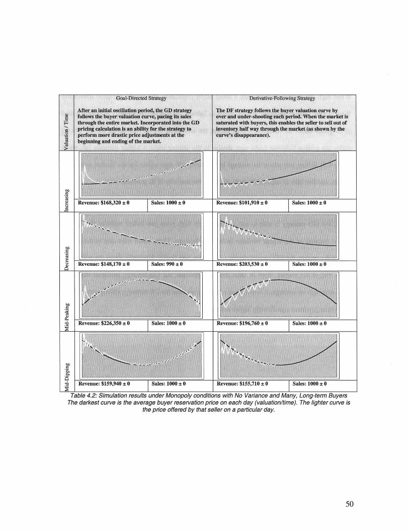
To provide a baseline for analysis, Table 4.2 contains the results of eight simulations with one
seller in the market, first using the GD strategy and then the DF strategy. In each simulation, there
is zero variance within the buyers' daily price distribution and many, long-term buyers in the
market. The charts illustrate the characteristic behavior of the GD and DF strategies under each of
the buyer valuation curves. In these trials, the standard deviations are zero because there is no
randomness to the results when there are numerous buyers in the market and there is no variation
between the buyers.
Shown in the left column of Table 4.2, the GD strategy follows each buyer valuation curve very
closely after a brief oscillation period. If the seller still has inventory to sell on the last days of the
market, the GD strategy results in another period of price oscillation in order to sell the remaining
inventory. While the strategy succeeds in finding and following the demand curve, this is not
always the best approach to the market. For example, in the case of constantly decreasing
valuation over time, the GD seller paces its sales to include sales on the worst days of the market.
Reflecting this poor behavior, this is the only case in which the GD strategy earned less revenue
than the DF strategy.
The DF strategy also successfully follows each buyer valuation curve, but in a pattern of over-
and under-shooting, shown in the right column of Table 4.2. When there is no variance in a large
buyer population, the DF strategy sells its entire inventory at the halfway point through the
market, and depending on the valuation curve, this is often not to the strategy's benefit. Only in
the case of decreasing buyer valuation over time, where it is to the seller's advantage to sell
during the first half of the market, did the DF strategy out perform the GD strategy.
The effect of variance within the buyer population is shown in Table 4.3. In the sample pricing
chart, both strategies adjust their pricing curves to be higher than the average buyer price, thereby

capturing the buyers who are willing to pay the highest prices each day. Again, the DF strategy
prevails on the decreasing valuation curve because it does not sell goods at the last, i.e. worst,
days of the market, unlike the GD strategy. Comparing these results to the initial case with no
price dispersion between the buyers, both strategies produce significantly more revenue for the
sellers under each valuation curve because they are able to raise their prices to meet the demand
of the buyers willing to pay higher prices on a single day.
Table 4.4 presents the simulation results when there are the same number of buyers in the market
as goods (1000) and the buyers each have a lifetime of one day, limiting the number of
opportunities a seller has to make a sale. As the results show, under most curves, the GD strategy
sells a significantly larger amount of inventory than the DF strategy, but this does not always lead
to higher total revenue. The sample pricing chart demonstrates the behavior of the two strategies
under the mid-peaking valuation curve. The GD strategy falls far below the buyer valuation curve
when sales are slow, and near the end of the market drops the price down to $1 in an attempt to
sell the remaining inventory. While it does manage to sell inventory, it does not do so at the best
price! Conversely, the DF strategy follows the curve closely as it has during the previous trials
and manages to maximize revenue per seat over the course of the market. Shown in the mid-peak
valuation curve, the DF strategy has achieved almost perfect matching of the valuation curve.
Examining the revenue results, the DF strategy produces more revenue than the GD strategy
except in the case of mid-peaking where the GD strategy managed to sell almost its entire
inventory at a mediocre price, while the DF strategy only sold two-thirds of its inventory.
When the market is severely limited in the number of buyers, the contrasting approaches of the
strategies demonstrate strengths and weaknesses. The GD overcompensates for the shortage of
buyers and sacrifices daily revenue for daily sales. If it can manage to sell its entire inventory,
then the total revenue makes up for the sacrifice. The DF strategy, by focusing on revenue per
good, consistently makes sales on each day of the market, at the highest possible price which can

eliminate lower-paying buyers. When it is able to sell a large percentage of its inventory, the total
resulting revenue is high.
When high variance is coupled with a small buyer population, the results are quite interesting.
What is most notable about the results shown in Table 4.5 is that the DF strategy sells only a third
of its goods under all valuation curves except the increasing curve. Examining the DF pricing
curve, the pricing behavior looks very similar to the pricing under a higher variance (shown in
Table 4.3), falling just above the average buyer curve. DF does adjust for the limited number of
buyers, and this lack of adjustment costs the seller the majority of its potential sales.
Contrast this result with the performance of the GD strategy. Referring to the sample pricing
curve, the GD strategy is able to sell at a relatively high price just before midway through the
market because of the higher variance in buyer valuations. Then, when sales slip in the second
half of the market, the GD strategy keeps a low price, and finally drastically drops the price to $1
at the end of the market. Both in sales and total revenue, the GD strategy performs extremely
well. Although on average, it is selling at a lower price than the DF strategy, selling over 90% of
its revenue produces significantly higher revenue.
Revenue: $168,320:* 0 Sales: 1000:* 0 Revenue: $101,910t* 0 Sales: 1000t* 0
Revenue: $148,170 * 0 Sales: 990 t 0 Revenue: $203,530 t 0 Sales: 1000 * 0
RRRevenue: $226,350:t 0 Sales: 1000:t 0 Revenue. $196,760 t 0 Sales: 1000t± 0
~_
Revenue: $159,940 ± 0 Sales: 1000 ± 0 Revenue: $155,710 ± 0
Cu
U
U
Table 4.2: Simulation results under Monopoly conditions with No Variance and Many, Long-term BuyersThe darkest curve is the average buyer reservation price on each day (valuation/time). The lighter curve is
the price offered by that seller on a particular day.
Sales: 1000 ± 0
oo

ValuationCurve:
Revenue: Sales: Revenue: Sales:
Increasing $199,680 ± 149 1000 ± 0 $149,036 ±1089 1000 ± 0Decreasing $208,673 ± 847 994 ± 7 $228,689 ±1078 1000 ± 0Mid-Peaking $275,052 ± 601 991 ±2 $243,633 ± 1228 1000 ± 0Mid-Dipping $202,006 ±198 1000 ± 0 $189,358 ± 739 1000 ± 0
Table 4.3: Monopoly with High Variance and Many, Long-term BuyersThe darkest curve is the average buyer reservation price on each day (valuation/time). The lighter curve is
the price offered by that seller on a particular day.
Sample PricingChart
ValuationCurve:
Revenue: Sales: Revenue: Sales:
Increasing $79,176 ± 4598 814 ±16 $123112 ±2690 790 ±13Decreasing $107,441 ± 2642 811 ± 13 $111,492 ± 2759 710 ±15Mid-Peaking $162,147 ± 5530 955 ± 7 $144,724 ± 3497 641 ±14Mid-Dipping $66,936 ± 2788 $740 ±16 $120,720 ± 2398 782 ± 12
Table 4.4: Monopoly with No Variance and Few, Short-term BuyersThe darkest curve is the average buyer reservation price on each day (valuation/time). The lighter curve is
the price offered by that seller on a particular day.
ValuationCurve:
neverlue: aates. Ievenue:
Increasing $141,958 ± 4619 999 ± 3 $189,63 ± 4114 977 ± 22Decreasing $127,302 ± 2107 889 ± 13 $67,333 ± 4180 328 ± 21Mid-Peaking $207,286 ± 2036 972 ± 5 $85,747 ± 5860 335 ± 24Mid-Dipping $102,601 ± 4409 907 ± 17 $75,253 ± 4669 372 ± 25
Table 4.5: Monopoly with High Variance and Few, Short-term BuyersThe darkest curve is the average buyer reservation price on each day (valuation/time). The lighter curve is
the price offered by that seller on a particular day.
Iaates:-

4.3 Competition: Two Sellers in the Market
In a competitive marketplace when sellers compete for market share, adaptive pricing strategies
react to the other strategies in the marketplace, not just the buyers' demand. Initially a market
scenario is presented in which none of the buyers compare prices across sellers or treat the sellers
different. Next the effects of comparison-shopping and seller-preference are presented. As in the
monopoly setting, each of the pricing charts in the following tables are based on a 100 day
simulation with the buyer valuation ranging from $100 to $300, depending on the valuation/time
curve. In each of the competitive simulations, there were 2000 buyers, the same number of total
goods in the marketplace.
Table 4.6 presents three different competitive pairings: Goal-Directed vs. Fixed-Price,
Derivative-Following vs. Fixed-Price, and Goal-Directed vs. Derivative-Following. The actual
success of a fixed-price seller depends on the fixed price it chooses. When used as a pricing
policy, a "fixed-price strategy" should be optimized based on the predicted behavior of the market
[12, 13]. The success of fixed-price strategies are not examined here, so the fixed-price has been
chosen to be $200, the average valuation over time, across all the valuation curves. The fixed-
price seller is presented as a way of demonstrating the interplay between the adaptive and fixed-
price strategies.
When the Fixed-Price seller is able to sell goods (when its price is below the buyer valuation
curve), the GD strategy stops adjusting its price and appears to mimic the Fixed-Price seller,
particularly under the increasing and decreasing valuation curves (Table 4.6, left column). The
reason the GD strategy stops changing its price is that when the Fixed-Price seller enters the
market, the sales are split between the two sellers, and in this case with 2000 buyers (1000 per
seller), the GD strategy sells the exact amount it aims to sell each day, making it unnecessary to
change the price. If there were more or less buyers in the market, the GD strategy would result in
a flat price curve at a higher or lower price point, respectively. Having a Fixed-Price seller in the

market prevents the GD strategy from finding the highest price the buyers are willing to pay, yet
in spite of this drawback, under every curve, the GD strategy produces a high amount of revenue
and sells almost its entire inventory.
When a DF strategy is paired with a Fixed-Price seller, center column of Table 4.6, it has
difficulty finding the buyer demand curve because of the low number of buyers and thus resorts
to more frequent, higher oscillations in price. When the Fixed-Price seller is not making any
sales, the DF strategy closely follows the buyer curve. This results in the DF strategy selling a
much higher percentage of its goods, but at much lower prices than the Fixed-Priced seller. Under
some curves this results in higher revenue for DF than for a Fixed-Price seller.
When DF and GD strategies are combined into the same marketplace, they do not respond to each
other in a dramatic way. In fact, the individual strategies in the right column of Table 4.6 look
much like when these strategies compete against a Fixed-Price seller, except because both
strategies are actively selling every day, the strategies never behave as they would with numerous
buyers in the marketplace. Each strategy is responding to the lack of buyers in the marketplace -
the GD strategy starts to drop prices as sales drop off and the DF strategy keeps raising the price
until it no longer makes sales and then dramatically lowers the price again.
When a population of comparison shoppers is added to the marketplace, there is much more
interaction between the two strategies. Table 4.7 compares the competitive effects of pairing two
Goal-Directed strategies, two Derivative-Following strategies, and one Goal-Directed strategy
with one Derivative-Following strategy when 100% of the buyer population compares the prices
of the two sellers and purchases from the lowest priced seller. When this trial was run with 75%,
50% and 25% comparison shoppers, the results linearly approached those with no comparison-
shopping.
Across the results, the amount of revenue earned by each seller has been dramatically reduced.
Examining the results of the two GD strategies, they behave much as they did in a monopoly
setting with limited buyers (Table 4.4), except they do not respond to the high variance in the
buyer population. The center column shows the two DF strategies, and as shown most
dramatically by the sample pricing curve, when they are paired together, they produce a price
war. Especially for the case of increasing valuation over time, the DF strategies drop their prices
to $1. When one GD competes with one DF, there is a modified price war, where prices don't
drop as dramatically, but are still forced down by the DF strategy. The DF strategy sells
approximately the same amount of inventory as GD, yet earns more revenue than the GD strategy
under all valuation curves and increases its revenue as compared to the DF-DF competition. This
occurs because the DF strategy does not limit the amount of inventory it sells at the beginning of
the market when prices are higher, while the GD strategy spreads out its sales, including selling
on the last days of the price war when prices approach zero.
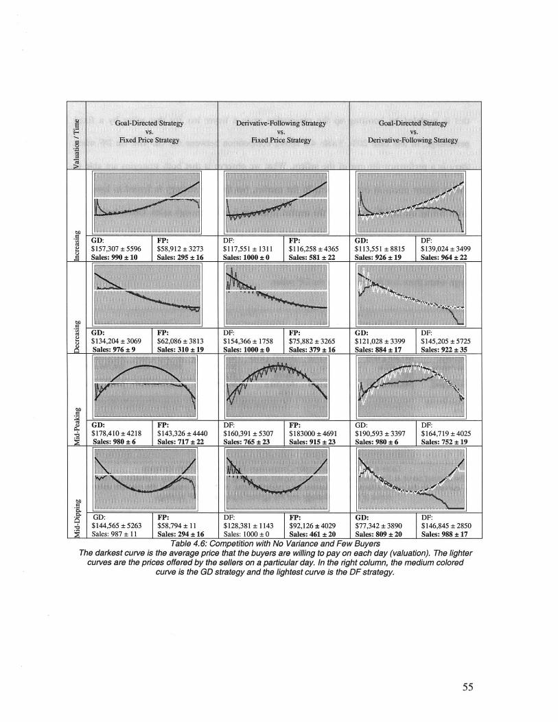
GD:$157,307 ± 5596Sales: 990:t 10
$134,204 ± 3069
GD:$178,410 ± 4218Sales: 980 ± 6
GD:$144,565 ± 5263Sales: 987 ± 11
FP:$58,912 ± 3273Sales: 295 *16
FP:$62,086 3813Sales: 310 ± 19
FP:$143,326 ± 4440Sales: 717 ± 22
FP:$58,794 ± 11Sales: 294 ± 16
DF:$117,551 ± 1311Sales: 1000* 0
$154,366 ± 1758Sales: 1000 + 0
DF:$160,391 ± 5307
DF:$128,381 ± 1143Sales: 1000 ± 0
FP:$116,258 ± 4365Sales: 581 * 22
FP:$75,882 ± 3265Sales: 379 * 16
FP:$183000 ± 4691qnIP- 91 ; + 23
FP:$92,126 ± 4029Sales: 461 ± 20
GD:$113,551 ± 8815Sales: 926± 19
$121,028 ± 3399Sales: 884 ±17
GD:$190,593 ± 3397
GD:$77,342 ± 3890Sales: 809 ± 20
DF:$139,024 ± 3499Sales: 964 ±22
DF:$145,205 ± 5725Sales: 922 ± 35
DF:$164,719 ± 4025Sales: 752 ± 19
DF:$146,845 ± 2850Sales: 988 ± 17
Cu
-I
Table 4.6: Competition with No Variance and Few BuyersThe darkest curve is the average price that the buyers are willing to pay on each day (valuation). The lighter
curves are the prices offered by the sellers on a particular day. In the right column, the medium coloredcurve is the GD strategy and the lightest curve is the DF strategy.
2
5

When buyers have a preference for a certain seller, the population of buyers considers that seller's
product to be more valuable, perhaps because of brand, quality, or reputation. In the simulator,
this is modeled by boosting up the reservation price a buyer has for that seller by a fixed
percentage, in this case 20%. Table 4.8 shows competition between the GD and the DF when
there is a preference for one of the sellers. What we observe is that both strategies are able to
charge higher prices at certain points in the market, but the GD strategy is forced to lower its
price during the middle portion of the market to ensure it made enough sales. Under both trials,
the sellers sold approximately 70-80% of their inventory. While the preferred seller earns more
revenue under the different trials, the earnings spread between the two sellers is not nearly as
large when there is a preference for the DF seller.
GD vs. GD DF vs. DF GD vs. DFWith Comparison-Shopping With Comparison-Shopping With Comparison-Shopping
Valuation GD Revenue: D Revenue: DF Revenue: DF Revenue: GD Revenue: F Revenue:Curve:Increasing $57,881 ± 2220 $57,881 ± 2220 $40532 ± 8211 $40532 ± 8211 $35,639 ± 2831 58,713 ± 1856Decreasing 87,058± 1875 $87,058 ±1875 $86512 ±6549 $86512 ±6549 71,826 ± 3564 117,151±4074Mid-Peaking 143,472 $143,472± $53,273 * $53,273 * 57,763 ± 4968 96,786 ± 3833
2837 2837 28,02 28,092Mid-Dipping
Sample PricingChart
$63,595 * 1664 $63,595 * 1664 $63,595 *I AM
$63,595 ±1 Ag
$50,765 ± 3939
Table 4.7: Competition under Comparison Shopping and High VarianceThe darkest curve is the average price that the buyers are willing to pay on each day (valuation). The lighter
curves are the prices offered by the sellers on a particular day. In the right column, the medium coloredcurve is the GD strategy and the lightest curve is the DF strategy.
Goal-Directed vs. Derivative-Following Goal-Directed vs. Derivative-FollowingWith Preference for GD With Preference for DF
ValuationCurve:Mid-PeakingSample PricingChart
GD Revenue: DF Revenue: GD Revenue: DF Revenue:
tInR R77+ -10. 1 r47 A7 + ATA10EA + 1% 4011 AA7 + A.
I aueI '1+.0. Lu"PLI/Iruon unaer a ouya r D IWfr r lor uIIterenL OersThe darkest curve is the average price that the buyers are willing to pay on each day (valuation). The
medium colored curve is the GD strategy and the lightest curve is the DF strategy.

4.3.1 Further Market Variation: Buyer Segmentation
Up until now the analysis of the strategies has been very controlled with the purpose of
discovering which market conditions effect a strategy's success. Now, both to continue the
strategy analysis and to demonstrate the richness to which the buyer behavior can be defined, an
analysis of the effect of buyer segmentation is presented. Buyer segmentation, or the dividing of
the simulator's buyer population into sub-groups, allows for different types of buyers to co-exist
in the market. As will be shown, the Goal-Directed strategy is better able to handle this type of
market diversity. To further illustrate the use of the simulator as an interface for analysis, the
results of this analysis are shown as screenshots from the simulator.
Strategies Sellers
A B
Fixed Price 0 0Goal Directed @ 0Goal Directed Quantity 0 0Derivative Following o @
Figure 4.9: Seller Strategies used in Trials 1 and 2.
Two trials were run, one with buyer segmentation, Trial 2, and one without, Trial 1. -The market
scenario for Trial 1 is presented in Figure 4.10. This is very similar to the market scenario
analyzed in the previous sections of this chapter: there are two sellers, 100 days, 1000 goods per
seller, and 4000 buyers. In the first trial, there is no buyer segmentation. In Trial 2, there is a
75/25 split to the buyer population, selected from the pull-down menu on the Market Scenario
screen (Figure 4.11). The two sellers in the trials each used the Goal-Directed and Derivative-
Following strategies, as shown in Figure 4.9.
Figure 4.12 shows the input screens for the two segments of the buyer population. Segment A, on
the left side of Figure 4.12, is the buyer segment present in both trials. Segment B, on the right
side of Figure 4.12, is 25% of the buyer population in Trial 2. Segment A could be described as
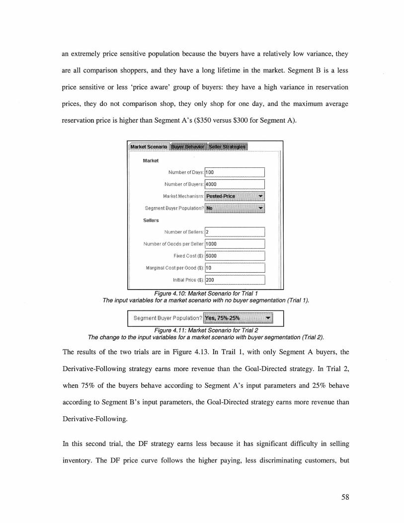
an extremely price sensitive population because the buyers have a relatively low variance, they
are all comparison shoppers, and they have a long lifetime in the market. Segment B is a less
price sensitive or less 'price aware' group of buyers: they have a high variance in reservation
prices, they do not comparison shop, they only shop for one day, and the maximum average
reservation price is higher than Segment A's ($350 versus $300 for Segment A).
market scenario
Market
Number of Days: 100
Number of Buyers: 4000
Market Mechanism: n Posted-Price
Segment Buyer Population? No
Sellers
Number of Sellers: 2
Number of Goods per Seller: 1000
Fixed Cost ($) 5000
Marginal Cost per Good ($) 10
Initial Price ($) 200
Figure 4.10: Market Scenario for Trial 1The input variables for a market scenario with no buyer segmentation (Trial 1).
Segment Buyer Population? Yes, 75%-25% |
Figure 4.11: Market Scenario for Trial 2The change to the input variables for a market scenario with buyer segmentation (Trial 2).
The results of the two trials are in Figure 4.13. In Trail 1, with only Segment A buyers, the
Derivative-Following strategy earns more revenue than the Goal-Directed strategy. In Trial 2,
when 75% of the buyers behave according to Segment A's input parameters and 25% behave
according to Segment B's input parameters, the Goal-Directed strategy earns more revenue than
Derivative-Following.
In this second trial, the DF strategy earns less because it has significant difficulty in selling
inventory. The DF price curve follows the higher paying, less discriminating customers, but
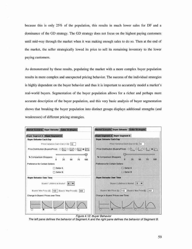
because this is only 25% of the population, this results in much lower sales for DF and a
dominance of the GD strategy. The GD strategy does not focus on the highest paying customers
until mid-way through the market when it was making enough sales to do so. Then at the end of
the market, the seller strategically lowed its price to sell its remaining inventory to the lower
paying customers.
As demonstrated by these results, populating the market with a more complex buyer population
results in more complex and unexpected pricing behavior. The success of the individual strategies
is highly dependent on the buyer behavior and thus it is important to accurately model a market's
real-world buyers. Segmentation of the buyer population allows for a richer and perhaps more
accurate description of the buyer population, and this very basic analysis of buyer segmentation
shows that breaking the buyer population into distinct groups displays additional strengths (and
weaknesses) of different pricing strategies.
Figure 4.12: Buyer BehaviorThe left pane defines the behavior of Segment A and the right pane defines the behavior of Segment B.
Bver Behador
Buyer Behavior Each Day
Price Variance Each Day (+4$) 10Price Distribution (Buyers/Price): 0 L 0 L
% Comparison Shoppers:0 25 50 75 100
Preference for Certain Sellers:
EI Seller A
E3 Seller B
Buyer Behavior Over Time
Buyers'Lifetime n Market 5
C Buyers Prices BuyersMax Price($).
Change in Buyers Prices over Time:

Figure 4.13: Simulator OutputThe left pane is the output from Trial 1 (one buyer population) and the right pane is the output from Trial 2(two differing buyer populations in one market). The pink (on the left) is the Goal-Directed strategy and the
green (on the right) is the Derivative-Following strategy.

4.4 Strategy Analysis Conclusions
While the Goal-Directed and Derivative-Following strategies are computationally basic, they are
surprisingly robust under extremely different market conditions. Under every case presented,
excluding the situation of 100% comparison-shopping, the strategies managed to adjust prices in
the direction of learning the changing demand in the marketplace, without knowing the true buyer
demand or competitors' prices. These strategies point towards some general guidelines for
choosing and designing adaptive pricing strategies:
* The Goal-Directed strategy consistently sells all or the majority of its inventory, given
any combination of buyer behaviors and competition, at the expense of drastically over-
and under-shooting the buyer valuation curve early and late in the market.
e The Derivative-Following strategy consistently sells at the highest price it can on any
single day. When there is a relative peak in demand during the first days of the market
and there is an abundance of buyers, DF performs very well. If buyer demand peaks at
some later time, DF does not space out its sales so as to insure that it sells a large number
of goods.
* In a monopoly, the shape of the valuation/time curve has an enormous effect on the
success of an individual strategy. Variance among buyer reservation prices and a limited
number of buyers requires the adaptive strategies to be more agile. When designing an
optimal strategy for a monopoly setting, knowledge about the typical valuation/time
curve and the buyer population should be incorporated into the pricing algorithm.
" If buyers are extremely price sensitive (100% comparison-shoppers), adaptive strategies
can easily break down into price wars. In particular, the Derivative-Following strategy
generated a price war between itself and other adaptive strategies.
* When there is product and seller differentiation (a willingness to pay more for certain
seller's products), a carefully designed adaptive strategy can narrow or widen the
discrepancy between the sellers' earnings.
* Buyer segmentation introduces complexities which can reverse the successes of a given
strategy. This highlights the importance of accurate modeling of a buyer population.
As dynamic pricing is deployed in markets, it is important to understand the interplay of different
pricing strategies. Deck, et al. in [11] compared two simple pricing strategies, price matching and
price cutting, and combined them into one simulated market setting, demonstrating that both
strategies were weakened in a mixed strategy marketplace. The strategies presented here, while
neither price matching nor cutting, produced mixed results. When there was no comparison-
shopping, the DF and GD strategies did not significantly effect each other's behavior or success
because these algorithms are not tied to competitor prices. But in the market with comparison-
shoppers (Table 4.7), the two strategies began to affect each other. The presence of a DF strategy
hurt the success of the GD strategy while the presence of the GD strategy improved the success of
the DF strategy over when it competed with another DF strategy.
Returning to the scenario of a ballpark selling baseball tickets, what dynamic pricing strategy
should a ballpark apply to its market to sell tickets at the highest demand levels while still filling
the park? Based on the market conditions of a ballpark (monopoly, high variance among the
buyers, and a low marginal cost per seat in the park), I would recommend using a strategy similar
to the Goal-Directed strategy. The Goal-Directed strategy's strength is its focus on selling the
entire inventory, sometimes at lower prices, which is a good approach under low marginal costs.
The Goal-Directed strategy also adjusts easily under high buyer variance, as shown in Table 4.3.
Under the conditions in Table 4.3, the GD strategy performs well under each valuation/time
curve. Actual market data from ballparks could provide us an accurate valuation/time curve

estimate to further inform a strategy choice. If one assumes the baseball ticket valuation curve
does not continuously decrease over time, then selling all the inventory at the beginning of the
market is to the ballpark's disadvantage, which a Fixed-Price policy or Derivative-Following
strategy does not protect against.
While the Goal-Directed calculation used in this analysis has not been optimized for the baseball
ticket market, the process of modeling a market and determining which adaptive strategy is most
successful is a useful exercise. The Learning Curve Simulator provides a mechanism for
analyzing pricing strategies, making the process of understanding and modeling a market a
straightforward task rather than a highly elusive problem.

64

5 Usage Analysis
In addition to building the Learning Curve Simulator for analyzing specific dynamic pricing
strategies, a secondary goal of this research is to create a tool that real-world sellers can use to
understand the potential impact of dynamic pricing on their markets. To evaluate the Learning
Curve Simulator in terms of its effectiveness as a tool for sellers, I conducted two informal
workshops during the MIT Media Lab's ThingsThatThink Consortium meeting, held in May
2001. Between eight and ten lab industry sponsors attended each workshop. After demonstrating
the usage of the Learning Curve Simulator, the sponsors and I explored different market
scenarios with the simulator, comparing a Fixed-Price strategy, the Goal-Directed strategy, and
the Derivative-Following strategy. Afterward, we discussed specific issues relevant to their
markets and explored how those factors would affect the results in the simulator.
5.1 Simulator as an Interface
The simulator interface received lots of positive feedback, both from people who had used market
simulators before and those who had not. Sponsors described the simulator as "clear" and
"uncluttered," with a good "separation of inputs and outputs."
Suggested improvements for the interface comprised requests for additional features such as the
ability to save a specific scenario and to compare results across simulation runs. Although not
demonstrated during the workshop, both of these actions can be done with the current simulator
by accessing the output file generated during each simulation. Comparative analysis can then be
done by hand, outside of the simulator application, by accessing the output file from a
spreadsheet application.
Other users requested adding mouse-over tool tips or hyperlinks that would explain more about
each variable in the simulator. If the simulator were to be released for general use, this would be

an excellent additional feature.
5.2 Simulator as a Tool
About half of the sponsors I spoke to stated that the simulator would be useful to their companies,
as it exists today. Several of them plan to access the simulator on-line or install it at their
company. They plan for employees involved in pricing decisions to use the simulator as a
learning tool. This was an extremely positive response, but there was still a desire among these
sellers for changes to the simulator.
Each sponsor I spoke to said the simulator would require more buyer behavior parameters to
accurately describe their market. Two specific types of buyer behavior mentioned by sellers were
"brand loyalty" and "different types of buyers." The current buyer behavior parameter
"preference for a certain sellers" is meant to express brand loyalty, but based on this feedback,
perhaps it does not do so clearly or effectively enough. While the request for different types of
buyers is vague, after this workshop I attempted to create that feature by adding the ability to
segment the buyer population into two distinct populations. This feature allows for a richer
description of the buyer population by creating two separate groups, which behave according to
two sets of buyer behavior parameters.
From talking to these sellers about their markets, my conclusion is that a general market simulator
cannot accurately model a company's market, because of the unique factors and perspectives each
company has. Instead, a general simulator is able to offer a higher level of understanding about
the effects of dynamic pricing. For a simulator to be a true reflection of a market and thus be a
tool the company can use to accurately predict the effect of a dynamic pricing strategy in their
own market place, a domain expert would need to incorporate historical and other market data
into the simulator's modeling of buyer behavior.

What I found to be most interesting when talking with sellers were the barriers they described
towards deploying dynamic pricing in their market. While it was a goal of each company I met
with, it was not something that could be implemented in the near future. For example, I spoke
with American Greetings about their season card division. Dynamic pricing is of great interest to
them, but they currently have several obstacles to implementation. First, they print the retail price
on all of their cards and then sell the cards in lots to retail stores at fixed prices. It is part of their
sales practice to always oversell the cards to retail stores, with the agreement that these stores are
able to return any unsold inventory for a full refund after the card's season. American Greetings
then sorts through the returned cards and puts a portion of the cards into storage for next year's
season. To preserve brand equity, it is a priority of American Greetings to never sell out of the
seasonal cards (Valentine's Day cards, for example).
By implementing dynamic pricing, American Greetings would be able to fine-tune the amount of
cards shipped to each retail store and then adjust the cards' prices to ensure that all inventory was
sold by the last day, but not before the last day. A strategy similar to the Goal-Directed strategy
might work for them because of its emphasis on inventory control. The company's current
inefficiency of accepting returned inventory and storing cards for the next year could be
eliminated with an effective dynamic pricing strategy.
While American Greetings sees the potential of dynamic pricing, they identify barriers to
implementation as 1) the current printing of prices on cards and 2) the current arrangement where
retail stores control the retail price, not American Greetings.
As a final observation, none of the sellers I spoke to criticized the limitation of the simulator only
modeling finite markets or the constrained set of seller strategies. Real-world markets will have
constraints on their parameters, whether or not they are related to a finite time horizon, and a
finite market is a specific way of expressing these constraints. During the workshops, I presented

only two pricing strategies, explaining that any strategy could be designed and implemented in
the simulator. The two we evaluated generated enough discussion and interest that I would
suggest that, when a company is performing a similar analysis of dynamic pricing options, two
strategies allow for enough diversity to understand the factors of dynamic pricing, without
overwhelming the analysis process.

6 Conclusion
Dynamic pricing will likely become a common competitive maneuver in the near future and
because of this, sellers need to be equipped with an understanding of how different pricing
strategies will play out in their marketplaces. A common type of market is one with a finite time
horizon, and it is in this market type that a seller has great potential to gain through adjustments
to price over time. In this thesis, I have presented a tool, the Learning Curve Simulator, for
modeling finite markets and for testing dynamic pricing strategies. By using such a simulator,
sellers can gain an understanding of dynamic pricing and of the different factors contributing to
successful dynamic pricing strategies.
There are several open issues in the deployment of dynamic pricing, for which the Learning
Curve Simulator can contribute towards solving. The following sections highlight some of these
issues in electronic markets and how a simulation-based approach can facilitate their solution.
6.1 Further Strategy Development
The adaptive pricing strategies implemented in this body of work illustrate one type of approach
to designing pricing strategies. There are many potential approaches to strategy development and
the simulator can serve as a platform for testing such strategies.
An effective technique for optimal pricing is dynamic programming [3] which, like revenue
management, makes assumptions about the marketplace to forecast and make optimal decisions,
taking into account time and inventory constraints. By considering the problem of pricing in a
market to be a multi-armed bandit allocation problem [20] and simplifying the strategy decision
to a finite number of decision variables, a strategy could be developed and tested in the Learning
Curve Simulator which found an optimal pricing solution for each market scenario. Although, as
discussed earlier, a drawback to this approach is the number of required market behavior
assumptions, such as the shape of the buyer valuation/time curve. Another drawback is that to
deploy an optimal solution, the calculation is often times too computationally intense for a real-
world setting [21]. But these drawbacks do not preclude the benefit of understanding how
dynamic programming strategies perform in a market and the Learning Curve Simulator can
provide the mechanism to do that.
6.2 More Realistic Buyer Behavior
As requested by the sellers who worked with the simulator, to make the simulator more effective
it needs more parameters to describe the behavior of buyers. In addition to the behaviors these
sellers suggested, there are additional behaviors that will occur in markets in response to the
introduction of dynamic pricing, and these behaviors should be modeled in order to understand
the impact of different pricing strategies. Just as leisure travelers often purchase airline tickets
more than twenty-one days in advance to receive a discounted fare, when sellers implement
dynamic pricing into new markets, discount-seeking buyers will work within the pricing rules to
receive a lower price. If the pricing strategy is not easily decipherable, buyers may change their
behavior in response to seeing prices change. For example, buyers sensitive to changing prices
may wait on a purchase if prices are falling or choose to buy immediately if prices are increasing.
The effect of this type of behavior on a strategy's success could be evaluated in a simulator that
accurately modeled the different ways in which buyers respond to dynamic pricing.
6.3 Buyer Response
Amazon.com's foray into dynamic pricing illustrated, perhaps too clearly, the risk of a negative
buyer response to buyer pricing. Amazon.com charged new customers less for a DVD than loyal
customers, and this initiated a widely publicized negative response from their customers.
There are several theories as to how Amazon.com could have avoided this backlash. One
proposal is that Amazon.com could have customized the entire sales package, including delivery

time, to create a qualitatively, versus quantitatively, better package [16]. While this would help
disguise the dynamic pricing, this would not have changed the basic fact that Amazon.com gave
benefits to new customers, not old ones. Another suggestion is that Amazon.com practice better
customer relations, through better follow-up and explanation of their pricing [2]. Again, I see this
as a patch to the problem that customers are upset that Amazon.com is discriminating against
their loyal customers.
My proposed recommendation for sellers implementing dynamic pricing is to publish or make
known the parameters by which the sellers change prices. Airlines and other industries such as
hotels and rental cars employ complex pricing strategies - while the strategies themselves are not
revealed, the rule that prices change over time and over type of traveler is well understood by
consumers and does not raise objections. Personalized pricing, or price discrimination, is more
complex than simply changing prices over time (as shown by Amazon.com). But today, when
sellers offer a discount to customers who sign-up for a particular promotion, customers
understand this rule and either elect to put themselves in that discounted customer segment, or
not. When rules are public, strategies will have to take into account the movement of buyers from
the non-discounted segment to the other, but this can be accommodated for with accurate
modeling of the movement of buyers between segments. While the current version of the
Learning Curve Simulator is not designed to model different buyer reactions to dynamic pricing,
a market simulator can be useful in understanding the potential outcomes of a negative response
to a pricing strategy or of a shift of buyers between different population segments.
6.4 Market Types
This thesis focused on finite markets with posted-prices, only briefly covering an auction
implementation. This constraint on the analysis does not limit the impact of the simulator as a
tool for understanding markets and dynamic pricing strategies. The lessons learned from finite
markets can be extended to markets with non-perishable goods, such as the automotive industry

[4, 9]. Pricing strategies could be designed to have knowledge of production and distribution
decisions and by changing prices could improve the entire supply chain.
Electronic markets allow for geographically distributed markets, and a by-product of this
distribution and the ability to make instantaneous price changes, is that auctions have become an
extremely popular market mechanism for selling products. While tempting to enter auction
markets to sell goods, sellers should proceed with caution when deploying dynamic pricing
strategies in these markets. Consumers behave differently in markets in which they name their
own prices and affect the sale price of the item [1]. Before developing a pricing strategy for an
auction, a seller should gather an understanding of how their customers will behave within the
chosen auction type. The Learning Curve Simulator could serve as a platform for modeling this
buyer behavior and studying the effects of this behavior on different auction pricing strategies.

References
1. Ariely, D. and Simonson, I. "The Psychology of On-line Auctions (Working Paper)."
2001.
2. Baker, W.L., Lin, E., Marn, M.V. and Zawada, C.C. "Getting Prices Right on the Web."
The McKinsey Quarterly. (Number 2). 2001.
3. Bellman, R.E. Dynamic Programming. Princeton University Press, Princeton, 1957.
4. Biller, S., Chan, L.M.A., Simchi-Levi, D. and Swann, J. "Dynamic Pricing and the
Direct-to-Customer Model in the Automotive Industry." GM Research & Development
Center, 2000.
5. Boyd, E.A. "Airline Alliance Revenue Management." OR/MS Today. (October 1998).
1998.
6. Brooks, C.H., Fay, S., Das, R., MacKie-Mason, J., Kephart, J. and Durfee, E.
"Automated Strategy Searches in an Electronic Goods Market: Learning and Complex
Price Schedules." Proceedings of the ACM Conference on Electronic Commerce (EC
'99), Denver, CO (November 1999).
7. Brynjolfsson, E. and Smith, M. "The Great Equalizer? Consumer Choice at Internet
Shopbots (Working Paper)." July 2000.
8. Carmon, Z. and Ariely, D. "Focusing On The Forgone: How Value Can Appear So
Different To Buyers And Sellers." Journal of Consumer Research. (27 (3)). 360-370.
2000.
9. Chan, L.M.A., Simchi-Levi, D. and Swann, J. "Flexible Pricing Strategies to Improve
Supply Chain Performance (Working Paper)." Northwestern University, 2000.

10. Clay, K., Krishnan, R. and Wolff, E. "Pricing Strategies on the Web: Evidence from the
Online Book Industry." Proceedings of the 2nd A CM Conference on Electronic
Commerce (EC '00), Minneapolis, Minnesota (October 2000), 44-55.
11. Deck, C.A. and Wilson, B.J. "Interactions of Automated Pricing Algorithms: An
Experimental Investigation." Proceedings of the 2nd ACM Conference on Electronic
Commerce (EC '00), Minneapolis, Minnesota (October 2000), 77-85.
12. Gallego, G. and van Ryzin, G. "A Multiproduct Dynamic Pricing Problem and Its
Applications to Network Yield Management." Operations Research. vol. 45 (1). 24-41.
1997.
13. Gallego, G. and van Ryzin, G. "Optimal Dynamic Pricing of Inventories with Stochastic
Demand Over Finite Horizons." Management Science. vol. 40 (8). 999-1020. 1994.
14. Greenwald, A., Kephart, J.O. and Tesauro, G.J. "Strategic Pricebot Dynamics."
Proceedings of the ACM Conference on Electronic Commerce (EC '99), Denver, CO
(November 1999).
15. Guttman, R. and Maes, P. "Agent-mediated Integrative Negotiation for Retail Electronic
Commerce." Proceedings of the Workshop on Agent Mediated Electronic Trading
(AMET'98), Minneapolis, Minnesota (May 1998).
16. Kalin, S. "How Low Can You Go?" Darwin Online. (April 2001). 2001.
17. Kephart, J., Hanson, J. and Greenwald, A. "Dynamic Pricing by Software Agents."
Computer Networks. vol. 32 (6). 731-752. 2000.
18. Kephart, J.O. and Greenwald, A. "Shopbot Economics." Proceedings of the Fifth
European Conference on Symbolic and Quantitative Approaches to Reasoning with
Uncertainty, (July 1999).

19. Keskinocak, P. and Tayur, S. "Quantitative Analysis for Internet-Enabled Supply
Chains." Interfaces, Special issue on Operations Research in the e-Business Era. vol. 31
(March/April 2001). 2001.
20. Leloup, B. and Deveaux, L. "Dynamic Pricing on the Internet: Theory and Simulations."
ENS de Cachan, GRID, NR 00-14. 2000.
21. McGill, J.1. and van Ryzin, G. "Revenue Management: Research Overview and
Prospects." Transportation Science. vol. 33 (No. 2 (May 1999)). p. 233-256. 1999.
22. Morris, J. and Maes, P. "Sardine: An Agent-facilitated Airline Ticket Bidding System."
Proceedings of the Fourth International Conference on Autonomous Agents (Agents
2000), Barcelona, Catalonia, Spain (June 2000).
23. Morris, J., Maes, P. and Greenwald, A. "Learning Curve: Analysis of an Agent Pricing
Strategy Under Varying Conditions." Proceedings of the Conference on Artificial
Intelligence, Las Vegas, NV (June 2001).
24. Smith, B.C., Gunther, D.P., Rao, B.V. and Ratliff, R.M. "e-Commerce and Operations
Research in Airline Planning, Marketing, and Distribution." Interfaces, Special issue on
Operations Research in the e-Business Era. vol. 31 (March/April 2001). 2001.
25. Smith, M., Bailey, J. and Brynjolfsson, E. "Understanding Digital Markets: Review and
Assessment." in Understanding the Digital Economy, Brynjolfsson, E. and Kahin, B.
eds., MIT Press, Cambridge, MA, 2000.

![[5]Dynamic Pricing in the Presence of Strategic Consumers ...heuristic.kaist.ac.kr/cylee/xpolicy/TermProject/09/[5]Dynamic Pricing... · Dynamic Pricing in the Presence of Strategic](https://img.pdfslide.us/doc/110x75/5e69e77f03649e388952ac9f/5dynamic-pricing-in-the-presence-of-strategic-consumers-5dynamic-pricing.jpg)