Embed Size (px)
Citation preview
Research ArticleA Simplified Solution for Calculating the Phreatic Line andSlope Stability during a Sudden Drawdown of the ReservoirWater Level
Guanhua Sun1 Shan Lin12 Wei Jiang3 and Yongtao Yang 1
1State Key Laboratory of Geomechanics and Geotechnical Engineering Institute of Rock and Soil MechanicsChinese Academy of Sciences Wuhan Hubei 430071 China2University of Chinese Academy of Sciences Beijing 100049 China3College of Civil Engineering amp Architecture China Three Gorges University Yichang 443002 China
Correspondence should be addressed to Yongtao Yang scuhhc126com
Received 21 June 2017 Revised 6 September 2017 Accepted 8 January 2018 Published 6 February 2018
Academic Editor Qinghui Jiang
Copyright copy 2018 Guanhua Sun et al This is an open access article distributed under the Creative Commons Attribution Licensewhich permits unrestricted use distribution and reproduction in any medium provided the original work is properly cited
On the basis of the Boussinesq unsteady seepage differential equation a new simplified formula for the phreatic line of slopesunder the condition of decreasing reservoir water level is derived by means of the Laplacian matrix and its inverse transform Inthis context the expression of normal stress on the slip surface under seepage forces is deduced and a procedure for obtaining thesafety factors under hydrodynamic forces is proposed A case study of theThree Gorges Reservoir is used to analyze the influencesof the water level decreasing velocity and the permeability coefficient on slope stability
1 Introduction
During the normal operation of a dam a decrease in waterlevel is the main cause of bank slope failure [1] There aremany potential landslide sites that exist in the region of theThree Gorges Reservoir and these are generally triggered bychanges in the water level Landslides cause huge losses bothin terms of property and life For example the landslide thatoccurred on 13 July 2003 at Qiangjiangping on the ThreeGorges Reservoir claimed many lives and was responsible forconsiderable infrastructure losses The accident serves as aprofound warning [2 3] and strongly motivates further studyof this type of natural disaster Many studies have confirmedthat changing water levels are the main cause of landslideevents [2ndash9]
The Chinese government has invested considerableresources to ensure slope stability under normal operationand to prevent natural disasters such as landslides Duringthe landslide survey and design review of the Three GorgesReservoir some problems were identified and require fur-ther clarification First there is no scientific basis for thedetermination of phreatic lines A decrease in water level
is the most unfavorable situation in terms of slope stabilityand usually leads to landslides Furthermore a decreasein water level can cause seepage problems related to therate of water level decrease and the slopersquos permeabilitycoefficient Therefore the correct approach should focus onthe above-mentioned factors to determine the phreatic lineand on the seepage pressure to analyze the slope stabilityHowever most of the determination of phreatic lines isbased on the designerrsquos experience which may lead toincorrect stability calculations and safety risk assessmentThesecond problem is related to the calculation of water forceswhich is ambiguous For example both the seepage forceand the surrounding hydrostatic pressure are considered incalculations which cause repetition of the water forces inthe equations and hence introduce more uncertainty Thethird problem is related to the velocity of the decreasingwater level which is again not clearly defined in the slopestability calculation In the case of power generation orflood control the Three Gorges Reservoir releases water ina very short span of time Such action leads to a rapiddecrease in the water level and in some cases triggerslandslides
HindawiGeofluidsVolume 2018 Article ID 1859285 14 pageshttpsdoiorg10115520181859285
2 Geofluids
The determination of the phreatic line constitutes afree surface (unconfined) seepage problem in rock and soilmechanics In such a case the key calculation is to determinethe free surface that delimits the flow boundaries The freesurface can be found using nonlinear numerical techniquessuch as the finite difference method with adaptive mesh [10]and the finite element method with adaptive mesh [11] orfixed mesh [12] Among the proposed methods the extendedpressure (EP) method proposed by Brezis and Kinderlehrer[13] and further simplified by Bardet and Tobita [14] usingfinite differences is considered the simplest andmost efficientfor free surface calculation Through an extension of Darcyrsquoslaw the EP method substantially reduces the variationalinequalities which can then be applied for computation of thewhole domain By applying variational inequalities Zheng etal [15] and Chen et al [16] made significant contributionsin solving the slope and dam free surface seepage problemsTo improve the accuracy and computational efficiency of theEP method an iterative error analysis is used with the finitedifference equations [17] Considerable progress has beenmade in calculating the slope phreatic line especially throughnumerical analysis using the finite difference and finiteelement methods However such numerical methods arenot commonly used in engineering practice and are usuallyignored in soil mechanics as they are obtained throughcomplicated derivations and are challenging to implementTherefore there is a need for a simple and efficientmethod forpractical engineering applications and educational training
To explain the effects of water load on the slope stability toengineers and technicians the surrounding water pressure isintroduced by the Swedish Slice method calculated from thedrift properties Based on these experiments it is concludedthat the seepage force water weight on the soil slices and thesurrounding hydrostatic pressure act as balancing forces foreach other [18]
In slope stability analysis under a changingwater level theconventional slice method is the limit equilibrium methodThe uncertainty is usually applied to the interslice forcesafter eliminating the slice bottom normal compressive forceby the two equilibrium equations of a single slice [19]Afterwards the statically indeterminate problem of the slopelimit safety factor can be solved using methods such as theMorgenstern-Price method [20] Spencerrsquos method [21] theSwedish method [22] the Bishop simplified method [19]or the Janbu simplified method [23] Many slice methodshave demonstrated that the interslice force is importantin calculating the slope stability in statically indeterminateproblems [24] Such traditional slice methods are categorizedas local analysis methods
Alternatively other limit equilibrium methods can becategorized as global analysis methods including the graphicmethod [25] the variational method [26] and Bellrsquos globalanalysis method [24] In contrast to the other limit equi-librium methods Bellrsquos method considers the entire systeminstead of using a single slide bar as a research objectTherefore the interslice force is not required in this methodwhich offers a new way to solve the strict slice method The-oretically the distribution of the slip surface normal stress inglobal analysis methods should be easier to understand than
the distribution of interslice force in the Morgenstern-Pricemethod However this method has not received sufficientattention even in the summary provided by Duncan [27]Until 2002 researchers in many studies [4 28ndash30] have usedsimilar methods For example in Bellrsquos derivation processZhu et al [29] and Zhu and Lee [28] used quadratic inter-polation to solve the slip surface normal stress distributionand derive one variable cubic equation with an unknownsafety factor Zheng and Tham [30] used the Green formulato convert the relevant domain integral calculus to boundaryintegral calculus
Firstly this paper applies the Boussinesq unsteady seep-age basic differential equations and boundary conditions forderivation of the expression for the phreatic line duringdecreasing water level conditions The polynomial fittingmethod is used to simplify the formula because of its lowercomplexity For solving the effects of water load on the slopestability the surrounding water pressure is calculated fromthe drift property Finally the global analysis method isproposed to analyze the slope stability under seepage forcesA typical landslide in theThreeGeorges Reservoir is used as acase study to analyze the influential factors for slope stabilityduring conditions of decreasing water level
2 Phreatic Line Calculations
21 Fundamental Assumptions
(1) The aquifer is homogeneous and isotropic with infi-nite lateral extension
(2) The phreatic flow parallel to slope surface is causedby water level fluctuation and the rainfall infiltrationcauses the phreatic flow to be perpendicular to slopesurface
(3) The reservoir water level is decreasing at a constantspeed of 1198810
(4) The reservoir bank is considered as a vertical slopeThe reservoir bank within the declining amplitudeis much smaller than the ground and in order tosimplify this it is considered as vertical reservoir bank[5]
As shown in Figure 1 based on the Boussinesq equationand following the above-mentioned assumptions the differ-ential equation of diving unsteady motion can be expressedas
120597ℎ1015840120597119905 = 119870120583 1205971205971199091015840 (119867
120597ℎ10158401205971199091015840) (1)
where 1199091015840 and ℎ1015840 are two directions of local coordinates asshown in Figure 1 119867 is the aquifer thickness 119905 is time 119870 isthe permeability coefficient and 120583 is the specific yield whichis defined as the amount of water released as a result of gravityin a unit volume of saturated rock or soil and can be expressedas the ratio between the water volume released by the gravityand the rock or soil volume in saturated conditions
Eq (1) is a second-order nonlinear partial differentialequation with no general analytical solution however it can
Geofluids 3
x
h
Initial water level
Water level aer fluctuation
Initial phreatic line
Phreatic line aer fluctuation
Slope surface
Impervious surface or slip surface
ℎ
u(xt)
ℎxt
x
u (x t)
Figure 1 Calculation sketch of phreatic surface
be simplified into a linear problem The simplified methodassumes the aquifer thickness 119867 to be a constant and thevalue is selected as the mean value of the initial and enddiving thickness Therefore the simplified one-dimensionalunsteady seepage flow equation can be rewritten as
120597ℎ1015840120597119905 = 1198861205972ℎ101584012059711990910158402 (2)
where 119886 = 119870119867119898120583 the value of 119867119898 will be discussed inSection 23
22 Models Used in This Study As shown in Figure 1 at theinitial time 119905 = 0 and by assuming the change of water levelof the position 1199091015840 at time 119905 the water level of each point1199061015840(1199091015840 119905) can be calculated as
1199061015840 (1199091015840 119905) equiv ℎ101584000 minus ℎ10158401199091015840 119905 = Δℎ10158401199091015840 119905 (3)
where 1199061015840(1199091015840 119905) is the reservoir water level change at time 119905 andposition 1199091015840 in local coordinates ℎ101584000 is the water level slope inlocal coordinates and ℎ10158401199091015840 119905 is the reservoir water level in localcoordinates The change of water level at 119905 = 0 is 1199061015840(1199091015840 0) =ℎ101584000 minus ℎ10158401199091015840 0 = 0
The reservoir water level decreases at a speed1198810 After thelateral seepage at 1199091015840 = 0 1199061015840(0 119905) = ℎ101584000 minus ℎ10158400119905 = 1198810119905 cos120572 as1199091015840 rarrinfin 1199061015840(infin 119905) = 0
From (3) the above semi-infinite aquifer groundwaterunsteady flow during the decreasing water level can besummarized by the following mathematical equations
1205971199061015840120597119905 = 1198861205972119906101584012059711990910158402 0 lt 1199091015840 lt infin 119905 gt 0
1199061015840 (1199091015840 0) = 0 0 lt 1199091015840 lt infin1199061015840 (0 119905) = 1198810119905 cos120572 119905 gt 01199061015840 (infin 119905) = 0 119905 gt 0
(4)
By applying the Laplace transform to (4) solving theequations and applying the inverse transform [31 32] the
10908070605040302010
252151050
M(
)
Figure 2 The curve of the function119872(120582) with 120582 (Formula (9))
solution of the differential equation can be mathematicallyexpressed as
1199061015840 (1199091015840 119905) = 1198810119905 cos120572 [(1 + 21205822) erfc (120582) minus 2radic120599120582119890minus1205822] (5)
where 120582 = 11990910158402radic119886119905 = (11990910158402)radic120583119870119867119898119905 and erfc(120582) =(2radic120587) intinfin
120582119890minus119909101584021198891199091015840 is the residual error function
By assuming (6) and following Figure 1 and (7) theequation can be rewritten as (8)
119872(120582) equiv (1 + 21205822) erfc (120582) minus 2radic120599120582119890minus1205822 (6)
119906 (119909 119905) = 1199061015840 (1199091015840 119905)cos120572 (7)
ℎ119909119905 = ℎ00 minus 1198810119905119872 (120582) (8)
which is the formula of the phreatic line of the slope whenthe reservoir water level declines at a constant speed 1198810 Thefunction 119872(120582) can be calculated by (6) and its curve isshown in Figure 2 According to (6) integral calculation isrequired which is difficult to perform and not convenient forengineering applications To obtain a practical expression for
4 Geofluids
x
h
Initial water level
Water level aer fluctuation
Initial phreatic line
Phreatic line aer fluctuation
Impervious surface or slip surface
Slope surface
o
a
b
c
R
Figure 3 Calculation sketch of aquifer thickness
engineering applications a polynomial fitting of (2) is usedas shown in Figure 2 which is simplified to [18]
119872(120582)=
01091205824 minus 07501205823 + 19281205822 minus 22319120582 + 1 (0 le 120582 lt 2)0 (120582 ge 0)
(9)
Afterwards the simplified formula of the phreatic lineunder a constant declining speed can be obtainedThe resultsfrom this formula are consistent with those from the finiteelement method under the same conditions which verifiesthe accuracy of this formula The expression can be writtenas
ℎ119909119905 = ℎ00 minus 1198810119905 (01091205824 minus 07501205823 + 19281205822 minus 22319120582 + 1) (0 le 120582 lt 2)ℎ00 (120582 ge 0) (10)
where 120582 = (119909cos1205722)radic120583119870119867119898119905 119870 is the permeabilitycoefficient (md) 119867119898 is the aquifer thickness (m) 120583 is thespecific yield 119905 is the time of the water level decrease (d) andℎ00 is the reservoir water level before it began to decline
23 Determination of the Aquifer Thickness For solving (1)the value 119867119898 is selected as the mean value of the initialand final diving flow thickness to replace 119867 during thelinearization and 119867119898 is referred to as the aquifer thicknessof the diving streamThis assumption is reasonable when thedrop height is relatively small but causes larger error whenthe drop height is relatively largeThus the followingmethodis used to determine the aquifer thickness For the irregularimpermeable layer as shown in Figure 3 the average aquiferthickness is not as simple as above and this often causes aproblem in engineering practice As a result it is necessary topropose a method that is convenient for use in engineeringapplications
For depicting the geological conditions of the ThreeGorges Reservoir the land surface component usually con-sists of weathered soils and collapsed accumulated bodiesoverlying rock Such geological conditions lead to gravellysoil forming in the upper part and a geological rock structurein the lower part The permeability coefficient of the rockis very small compared to the soil Thus the former can beneglected and the combined surface between the rock andsoil can be used as an impermeable layer The cross-sectionis shown in Figure 3 The calculation area is restricted by
the rock (impermeable layer) however when the reservoirwater level drops the influential area cannot be used asthe horizontal impermeable layer In this case the followingmethod is promising for determining the average thicknessof the aquifer
Actual landslides do not have vertical slopes but ratherslope gradientsWhen the reservoir water level decreases theoverflow points are usually located on the steep slope surfaceand the flow follows the slope gradient In contrast thephreatic line on the slope is relatively flat In such situationsthe initial water level and slope line can replace the phreaticline in the calculation of the average aquifer thickness whichcan be calculated by the following equation
119867119898 = 119878119900119886119887119888119877 (11)
where 119878119900119886119887119888 is the area consisting of the slope surface 119900119886 theinitial water level 119886119887 the bedrock surface 119887119888 and the crosspoint between the water level drop and the slope surface 119900119888and 119877 is the intersection of the initial water level with thebedrock surface The geological section is often drawn usingCAD software [5 18]
24 Specific Yield Specific yield is an important hydroge-ological parameter that should be obtained through actualmeasurements It is defined as the amount of water releasedas a result of gravity in a unit volume of saturated rock orsoil and can be expressed as the ratio between the water
Geofluids 5
volume released by the gravity and the rock or soil volumein saturated conditions
In rock and soil only some pores are filled by water andmovement is possible through connected pores Such poresare generally termed as effective pores in hydrogeology Inhydrology or groundwater dynamics the effective porosityis the ratio between the pore volume filled by water andthe water released from gravitational pull and the total porevolume of these pores The effective porosity is generallycontrolled by the physical properties of the rocksoil It isoften expressed in terms of percentage
According to the test data of gravel and clayey soil [33]the empirical formula of specific yield is
120583 = 1137119899 (00001175)0067(6+lg119870) (12)
where 119899 is the porosity and 119870 is the permeability coefficient(cms) In the absence of experimental data (12) can be usedto calculate the specific yield
3 The Normal Stress in the Slip SurfaceInduced by Hydrodynamic Forces andSurface Water Forces
31 Seepage Force Calculation The drag force on the soilby water under seepage is known as the seepage force andis often described as a dynamic water force in engineeringSeepage force calculation is the key factor for evaluatingthe slope stability under seepage Thus the accuracy of theseepage force calculation strongly influences the results Itappears that engineers are often conceptually confused aboutthe seepage force and the surrounding hydrostatic forcecalculations in which the equation of the water forces isrepeated and the influence of the void ratio on seepageforce calculations To clarify these issues the calculationof the seepage forces can be studied in terms of thewater forces using the boundary of each differential slicethis is the most direct way to analyze the seepage forces[18]
The force diagram of a single soil slice is presented inFigure 4 In the diagram 1198891198821 and 1198891198822 are the saturatedsoil gravity components above and below the phreatic linerespectively The force 119875119886 is the hydrostatic force at the 119860119861border 119875119887 is the hydrostatic force at the 119862119863 border 119880 is thehydrostatic force at the 119861119862 border 119873 is the normal forceat the base which is also known as the effective force 120572is the angle between the bottom surface and the horizontaldirection and 120573 is the angle between the phreatic line andthe horizontal direction
To determine the hydrostatic forces 119875119886 119875119887 and 119880 onthe 119860119861 119862119863 and 119861119862 borders the flow grid properties basedon the nature of drift and flow lines perpendicular to theequipotential lines are used In Figure 5 119861119864 and 119862119866 areperpendicular to the phreatic line 119866119867 is perpendicular to119862119863 and 119864119865 is perpendicular to119860119861 Thus the hydraulic head119861119865 in 119861 and the hydraulic head 119862119867 in C can be expressedaccording to geometric relationships
A
B
C
D
x
y
T
ℎw
dW1
ℎu
Pa ℎa
N + U
dW2
ds
ds cos
Pbℎb
Figure 4 Calculation sketch of differential soil slice
A
B
C
D
E F
HG
M
N
x
y
ℎa
ℎb
ds cos
Figure 5 Calculation sketch of hydraulic grade
119880119861 = ℎ119886cos2120573119880119862 = ℎ119887cos2120573
(13)
6 Geofluids
The resultant force of the hydrostatic force on the119860119861 and119862119863borders can be represented by
119875119886 = 12120574119908ℎ2119886cos2120573119875119887 = 12120574119908ℎ2119887cos2120573
(14)
The hydrostatic force on the sliding surface 119861119862 is representedby
119880 = 120574119908 (ℎ119886 + ℎ119887) 1198891199042 cos2120573 (15)
The forces in the vertical and horizontal directions can berespectively expressed as
119880119910 = 120574119908 (ℎ119886 + ℎ119887) 1198891199042 cos120572 cos2120573119880119909 = 120574119908 (ℎ119886 + ℎ119887) 1198891199042 sin120572 cos2120573
(16)
The water weight in the soil is
1198822119908 equiv 120574119908 (ℎ119886 + ℎ119887) 1198891199042 cos120572 (17)
where1198822119908 is the water gravity below the phreatic line of thesoil slice
By assuming
ℎ119908 equiv ℎ119886 + ℎ1198872 (18)
we obtain
119875119886 minus 119875119887 = 120574119908ℎ119908 (ℎ119886 minus ℎ119887) cos21205731199082119908 = ℎ119908120574119908119889119904 cos120572119880119910 = 120574119908ℎ119908119889119904 cos120572 cos2120573119880119909 = 120574119908ℎ119908119889119904 sin120572 cos2120573
(19)
All the water loads below the phreatic line in the soil sliceare shown in Figure 6 The 119909-direction component of all thewater loads is
119875119886 minus 119875119887 + 119880119909 = 120574119908ℎ119908cos2120573 (ℎ119886 minus ℎ119887 + 119889119904 sin120572) (20)
The 119910-direction component of all the water loads is
1198891198822119908 minus 119880119910 = 120574119908ℎ119908119889119904 sin2120573 (21)
From the geometrical relationships as shown in Figure 6 theequation can be represented as
ℎ119886 minus ℎ119887 + 119889119904 sin120572 = 119889119904 cos120572 tan120573 (22)
Therefore the forces from all water loads become
119889119882119863 = 120574119908ℎ119908119889119904 cos120572 sin120573 (23)
A
B
C
D
x
y
N
T
dW1
dWD
dW1
Figure 6 Forces distributing diagrammatic sketch of differentialsoil slice
The geometrical interpretation of the full water immer-sion saturated area in the soil slice is that the water grav-ity and hydraulic gradient sin120573 are equal to the seepageforce and hydrodynamic force respectively The directionof this force is the same as the fluid flow direction andthe angle between the force and the horizontal direction is120573
This calculation demonstrates that the seepage force is thesame as the resultant forces of water gravity and surroundinghydrostatic force of the soil below the phreatic lineThereforewhen the seepage force is used to express the safety factor thenatural gravity is used above the phreatic line whereas thefloating gravity in this case is used below the phreatic lineTherefore the calculation diagram shown in Figure 2 can bereplaced by that in Figure 6 Additionally the water force andgravity of the soil slice can be replaced by the seepage force119889119882119863 As a result this type of problem is straightforward tosolve in practice
32 Normal Stress on the Slip Surface under the Water LoadsThe forces along the arc length ds in the antislide directionof the differential slice 119860119861119862119863 are shown in Figure 7 Theparameters 119889ℎ and 119889V are the interslice force incrementsin the horizontal and vertical slice respectively 119889119908 and 119889119902are the bar weight and seismic force respectively and 119889119891119909and 119889119891119910 are the components in the horizontal and verticaldirections on the outer contour line 119892 respectively Therelationship between the normal face force 119902119899 and tangentialforce 119902119905 is
119889119891119909 = 119902119905119889119909119892 minus 119902119899119889119910119892119889119891119910 = 119902119899119889119909119892 + 119902119905119889119910119892 (24)
where 119889119909119892 and 119889119910119892 are the 119909 and 119910 directional componentsalong the differential arc length 119889119904119892 in119892 as shown in Figure 7
Geofluids 7
A
B
C
D
dv
dh
ds
M
N
dW1
dW1
dWDx
dWDy
dsg
dfx
dfy
ds
ds
Figure 7 The schematic diagram of a loaded differential slice forderivation of normal stress on sliding surface
All the forces are projected on the normal direction of theslip surface thus the equation becomes
120590119889119904 = 1198891198821 cos120572 + 11988911988210158401 cos120572 + 119889119882119863119910 cos120572minus 119889119882119863119909 sin120572 + 119889119891119909 sin120572 minus 119889119891119910 cos120572+ 119889V cos120572 minus 119889ℎ sin120572
(25)
1198891198821 = 120574ℎ11990611988911990911988911988210158401 = 1205741015840ℎ119908119889119909 (26)
119889119882119863119909 = 119889119882119863 cos120573119889119882119863119910 = 119889119882119863 sin120573 (27)
where ℎ119906 is the bar height above the phreatic line 120574 is theaverage bar weight and 1205741015840 is the effective average weight
Substituting (24) (26) and (27) into (25) where 119889119909119892 =minus119889119909 we obtain120590 = 120590 (119909) = 1205900 + 120590119868 (28)
where 120590119868 and 1205900 are the contributions from the intersliceforces and external load to the normal stress in the slipsurface respectively and are generally expressed as a functionof 119909
120590119868 = cos120572( 119889V119889119909 cos120572 minus 119889ℎ119889119909 sin120572) (29)
The stress 1205900 is decomposed into
1205900 = 120590V0 + 1205901198920 (30)
where 120590V0 is the contribution from the slider body volumeforce to the normal stress in the slip surface
120590V0 = 120574ℎ119906cos2120572 + 1205741015840ℎ119908cos2120572 + 120574119908ℎ119908cos2120572 sin2120573minus 120574119908ℎ119908 sin 2120572 sin 21205734 (31)
Here 1205901198920 is the contribution from the water pressure of theouter contour slope slip surface to the normal stress in theslip surface
1205901198920 = cos120572 [119902119899 (cos120572 + 119896119892 sin120572)minus 119902119905 (sin120572 minus 119896119892 cos120572)]
(32)
where 119896119892 is the outer contour slope surface at point119872Usually the interslice forces V and ℎ at both ends of the
sliding surface are zero however their derivatives 119889V119889119909 and119889ℎ119889119909may not be zero Additionally from (28) and (29) theslip surface normal stress at both ends may not be zero eitherTherefore it is not necessary to satisfy the zero condition atthe slip surface ends when determining the normal stress atthe slip surface Hence the distribution of the slip surfacenormal stress approximation can be determined as shown in(33)
120590 = 1205900 + 119891 (119909 119886 119887) (33)
where 119891(119909 119886 119887) is the correction function for the slip sur-face normal stress and 119886 and 119887 are the two undeterminedparameters The reason for introducing two undeterminedparameters is that three equilibrium equations are used tosolve for three unknowns in which the safety factor 119865119904 is oneof the unknowns
In this study119891(119909 119886 119887) is defined as a linear function [30]119891 (119909 119886 119887) = 119886119897119886 (119909) + 119887119897119887 (119909)
119897119886 (119909) = minus 119909 minus 119909119887119909119887 minus 119909119886 119897119887 (119909) = 119909 minus 119909119886119909119887 minus 119909119886
(34)
where 119909119886 and 119909119887 are the 119909 coordinates of two endpoints onthe slip surface 119904 in this two-dimensional problem
4 Slope Stability Analysis Method underWater Loads
As shown in Figure 8 the slip body is defined as a planarregion Ω consisting of an outer contour line ACB and apotential slip surface ADB The background materials aregenerally formed by a variety of geotechnical movements atthe landslide sites The active forces of the landslide include
8 Geofluids
q
w
g
s
B
A
D
C
O
y
x
(x)
(x)
Ω
qn
qt
Figure 8 Schematic plot of a sliding body and system of forces on it
volume forces (eg weight and horizontal seismic forces) andthe concentrated force or surface force on the outer contourACB the constrained forces include the slip surface normalforce 120590(119909)119889119904 and the tangential force 120591(119909)119889119904
By taking any three points (119909119888119894 119910119888119894) which are not inthe same straight line as the moment center and with Ω inequilibrium the sum of the three moment centers is alwaysequal to zero and can thus be expressed as
int119878(Δ119909119888119894120590 minus Δ119910119888119894120591) 119889119909 + (Δ119909119888119894120591 + Δ119910119888119894120590) 119889119910 + 119898119888119894= 0
(35)
where 119898119888119894 is the resultant moment of all active forces on thelandslide bodyΩ 119894 = 1 2 3 and Δ119909119888119894 and Δ119910119888119894 are the vectorcomponents on the slip surface at position (119909 119910)
Δ119909119888119894 = 119909 minus 119909119888119894Δ119910119888119894 = 119910 minus 119910119888119894 (35a)
If not specifically stated all subscripts 119894 in the equationsare free subscripts In the formula 119894 will take the value of1 2 and 3 and provide three moment centers (119909119888119894 119910119888119894)Additionally to simplify the expression and by assuming theslope is the right-side slope it is found that an increase inslope height occurs with an increasing 119909 coordinate value
By assuming that the sliding surface meets the Mohr-Coulomb criterion and the landslide body is in the limitequilibrium state the equation can be written as
120591 = 1119865119904 [119888119890 + 119891119890120590] (36)
where 119865119904 is the safety factor and 119888119890 and 119891119890 are the effectiveshear strength parameters
By substituting (36) into (35) the unknown functionintegral equations of the sliding surface normal stress can beobtained as
int119878119871119909119888119894120590119889119909 + 119871119910119888119894120590119889119910 + 119898119888119894119865119904 + 119889119888119894 = 0 (37)
where
119871119909119888119894 = 119865119904Δ119909119888119894 minus 119891119890Δ119910119888119894119871119910119888119894 = 119865119904Δ119910119888119894 + 119891119890Δ119909119888119894 (37a)119889119888119894 = int
119878119888119890Δ119909119888119894119889119910 minus 119888119890Δ119910119888119894119889119909 (37b)
By substituting (33) into (37) (38) can be derived
g (119865119904 119886 119887) equiv 119865119904 (119886u1 + 119887u2 + u3) + 119886u4 + 119887u5 + u6 (38)
where g 1198773 rarr 1198773 is the third-order nonlinear vectorfunction of 119886 and 119887 and u1simu6 are the six third-order vectorswhich can be defined as follows
1199061119895 = int119878Δ119909119888119894119897119886119889119909 + Δ119910119888119894119897119886119889119910 (38a)
1199062119895 = int119878Δ119909119888119894119897119887119889119909 + Δ119910119888119894119897119887119889119910 (38b)
1199063119895 = 119898119888119894 + int119878Δ1199091198881198941205900119889119909 + Δ1199101198881198941205900119889119910 (38c)
1199064119895 = minusint119878119891119890Δ119910119888119894119897119886119889119909 minus 119891119890Δ119909119888119894119897119886119889119910 (38d)
1199065119895 = minusint119878119891119890Δ119910119888119894119897119887119889119909 minus 119891119890Δ119909119888119894119897119887119889119910 (38e)
1199066119895 = minusint119878(119888119890 + 1198911198901205900) Δ119910119888119894119889119909 minus (119888119890 + 1198911198901205900) Δ119909119888119894119889119910 (38f)
Equation (38) can be used as a quasi-Newton method tosolve [34] The required Jacobian matrix of g(119865119904 119886 119887) in thesolution can be defined as119863g
119863g (119865119904 119886 119887) equiv [119863g119865119904 119863g119886 119863g119887] (39)
Geofluids 9
Qianjiangping Landslide
Woshaxi Landslide
Qinggan River
Yangtze River
ree Gorges Dam
Yangtze River
Figure 9 The geographical location map of Woshaxi Slope in theThree Gorges Reservoir
where the three column vectors are expressed as
119863g119865119904 equiv 120597g (119865119904 119886 119887)120597119865119904 = 119886u1 + 119887u2 + u3 (39a)119863g119886 equiv 120597g (119865119904 119886 119887)120597119886 = 119865119904u1 + u4 (39b)119863g119887 equiv 120597g (119865119904 119886 119887)120597119887 = 119865119904u2 + u5 (39c)
In this study the following condition can be used toterminate iteration during numerical simulations and can beexpressed as
Δ119865119904 lt 120576119865119904 (40)
where Δ119865119904 is the difference between the two consecutiveiteration steps and 120576119865119904 is the selected tolerance level
In the following examples 120576119865119904 = 10minus3 is used as a dampedNewtonrsquos method [34] The landslide border is dispersed intoseveral small segment grids In the smaller grid segments theslip surface normal stress is assumed to be constant
5 Influence Factors of Slope Stability
For ease of analysis the drop height of the reservoir water isassumed to be ℎ119905 = 119881119905 (8) can then be rewritten as follows
ℎ119909119905 = ℎ00 minus ℎ119905119872(120582) 120582 = 119909 cos1205722 radic 120583119881119870119867119898ℎ119905
(41)
These equations indicate that the factors influencing thephreatic line under a decreasing water level include thepermeability coefficient119870 the specific yield 120583 the decreasingspeed of the water level 119881 the aqueous layer thickness 119867119898and the decreasing height ℎ119905 From Figure 2 119872(120582) is adecreasing function inversely related to 120582 A higher 120582 valuecauses a reduction in the speed of the free surface water flow
and vice versa Therefore when 120582 = 0 119872(120582) = 1 and thespeed of the free surface water on the slope and the waterlevel become equal When 120582 rarr infin119872(120582) = 0 and the freesurface water on the slope and the water level are unchangedIt is clear from Figure 2 that when 120582 gt 2119872(120582) becomes 0
The higher water level on the slope causes an unfavorablecondition for the slope stability Based on the above analysisthe smaller 120582 is the faster the free surface water flow on theslope is which means the free surface water decreases withdecreasing water level and vice versa Similarly the larger 120582values cause unfavorable conditions for the slope stabilityThe favorable factors for the slope stability are the decreasein 120582 directly related to the decreasing rate of the water level119881 the permeability coefficient 119870 the specific yield 120583 andthe water thickness119867119898 Most engineers generally analyze theeffects of decreasing rate of water level 119881 and permeabilitycoefficient 119870 on the slope stability
The Woshaxi landslide occurred on 13 July 2003 at theright bank of Qinggan River a tributary of the YangtzeRiver The Qinggan River flows from west to east and passesin front of the landslide site The landslide was located6 km from the mouth of the river The distance from thedownstream Qinggan River to the Qianjiangping landslidesite is approximately 15 km (Yin et al 2012 Wang and Li2007Wand and Yang 2006Wen et al 2008Wu et al 2006Yin and Peng 2007 Zhang et al 2004 Jian et al 2014) [2ndash4 6]The distance to theThree Gorges dam site is 50 kmThegeographical position of the landslide is shown in Figure 9
The geological cross-section is shown in Figure 10 andthe geologicalmaterials are listed in Table 1TheThreeGorgesReservoir water level is found to be between 145m and 175mThis study evaluates the landslide stability associated with thedecreasing water level from the height of 175m Below thephreatic line the soil saturation density is used and for thenatural strength of slip the soil above the phreatic line is used
Using different decreasing water level speeds the otherrelated parameters are shown in Table 1 Figure 11 showsthe calculation process for the phreatic line under differentdecreasing water level rates Figure 11(a) indicates the changein the phreatic line for different water level conditions and a
10 Geofluids
Table1Parameterso
fWoshaxiSlop
e
Weightu
nit
120574(KNm3)
Shearstre
ngth
Perm
eability
coeffi
cient
119870(md)
Specificy
ield
120583Uncon
fined
aquifer
thickn
ess
119867 119898(m
)Saturated
cond
ition
Natural
cond
ition
Saturatedcond
ition
Naturalcond
ition
119888 119890(kPa)
120593(∘)
119888 119890(kPa)
120593(∘)
224
208
1815
2220
010
001
65
Geofluids 11
380360340320300280260240220200180160140120100
Elev
atio
n (m
)
380360340320300280260240220200180160140120100
Elev
atio
n (m
)175145
Landsliding mass
500 100
Bed rock
(m)
Figure 10 The geological section map of Woshaxi Slope
100 200 300 400 500 600 700(m)
100
150
200
250
300
350
(m)
145
175
(a) 119881 = 01md
100 200 300 400 500 600 700(m)
100
150
200
250
300
350
175
145(m
)
(b) 119881 = 04md
100 200 300 400 500 600 700100
150
200
250
300
350
175
145
(m)
(m)
(c) 119881 = 12md
Figure 11 Phreatic lines of reservoir drawdown height with different drawdown speed
decreasing water level rate (119881) of 01md Figure 11(b) showsthe phreatic line for differentwater levels at a decreasingwaterlevel rate of 119881 = 04md Figure 11(c) shows the phreatic linefor different water level conditions and a decreasing waterlevel rate of 119881 = 12md The safety factors under differentwater levels at different decreasing water level rates are shownin Figure 12When the decreasing water level rate is relativelysmall there is sufficient time for the water in the slope todischarge from the slope which causes a slow change in thephreatic line as shown in Figure 11(a) When the decreasingwater level rate is relatively high there is insufficient timefor the water on the slope to discharge causing a suddenchange in the phreatic line as shown in Figure 11(c) Thedecreasing water level rate has a profound effect on thephreatic saturation lines and therefore on the slope safetyfactors As shown in Figure 12 a more obvious change isobserved in the safety factors as the water level slightlydecreases however no significant changes are observed in thesafety factors when the water level decreases by a substantial
margin Overall as the decreasing water level rate increasesit causes a decrease in the safety factor It is further observedthat at a given decreasing water level rate the safety factortends to be more stable with an increase in water level Itis found that when the height of the reservoir water leveldecreases from 175m to 145m a 5 change is observed inthe safety factor at decreasing water level rates of119881 = 01mdand 119881 = 12md
In the current study the phreatic line is calculated byvarying the slope permeability coefficients at a constantwater level decreasing rate that is 119881 = 60md The otherparameters required for calculating the phreatic line are givenin Table 1 Figures 13(a)ndash13(c) and 14 show the phreatic lineand safety factors respectively under different water levelswhen the permeability coefficient 119870 is 001md 010mdand 100md respectively It can be observed that at thesame water level decreasing rate the variation in 119870 causesdifferences in phreatic line behavior With a relatively small119870 there is a sudden change in the phreatic line as sufficient
12 Geofluids
095
100
105
110
115
Safe
ty fa
ctor
s
172
5
170
167
5
165
162
5
160
157
5
155
152
5
150
147
5
145
175
Water level elevation (m)
01 md08 md02 md
12 md04 md
Figure 12 Effect of reservoir drawdown height on landslide stability with different drawdown speed
100 200 300 400 500 600 700100
150
200
250
300
350
175
145
(m)
(m)
(a) 119870 = 001md
100 200 300 400 500 600 700100
150
200
250
300
350
175
145
(m)
(m)
(b) 119870 = 010md
100 200 300 400 500 600 700100
150
200
250
300
350
(m)
(m)
175
145
(c) 119870 = 100 md
Figure 13 Phreatic lines of reservoir drawdown height with different permeability coefficient
time is not available for water to be transported down theslope (Figure 13(a)) However with increasing 119870 the changein the phreatic line is gradual because more time is availablefor the water to be transported down the slope (Figures13(b)-13(c)) The permeability coefficients have a profoundeffect on the phreatic lines and the slope safety factors Asshown in Figure 14 significant changes in the safety factorsoccur when the water level decreases slightly with differentslope permeability coefficients In contrast the safety factordoes not change substantially with large changes in the waterlevel Overall the slope permeability coefficient is inverselyproportional to the safety factor which indicates that an
increasing permeability coefficient can cause a decrease in thesafety factor A larger slope permeability coefficient impliesa higher safety factor It is also evident from this study thata decreasing water level leads to a more stable safety factorwhich can be ascribed to the slope permeability coefficientA larger slope permeability coefficient is associated witha greater probability of penetration with decreasing waterlevel which is favorable for slope stability It is clear fromthe results that when the height of reservoir water leveldecreases from 175m to 145m the difference in the safetyfactor is only approximately 6 at 119870 = 10md and119870 = 001md
Geofluids 13
095
1
105
11
115
Safe
ty fa
ctor
s
172
5
170
167
5
165
162
5
160
157
5
155
152
5
150
147
5
145
175
Water level elevation (m)
001 md010 md 100 md
050 md
Figure 14 Effect of reservoir drawdown height on landslide stabilitywith different permeability coefficient
6 Summary
(1) The expression of the phreatic line is based onthe Boussinesq unsteady seepage basic differentialequations and boundary conditions The polynomialfitting method is used to obtain a simplified formulathat is convenient to use in engineering applications
(2) To simplify the explanations and provide greaterunderstanding to engineers the flow grid propertiesare used to determine the water forces which demon-strates that the seepage and resultant force causedby the water weight in the soil and the surroundinghydrostatic forces balance each other
(3) The expression of the slip surface normal stress underthe dynamic water forces is derived and an equationfor solving the safety factor under different dynamicwater forces is proposed
(4) Combined with a practical project in the ThreeGorges Reservoir the effects of decreasing waterlevel rate and the slope permeability coefficient areanalyzed and presented to describe slope stability
Conflicts of Interest
The authors declare that they have no conflicts of interest
Acknowledgments
This study is supported by the National Natural ScienceFoundation of China [Grant no 11572009] and the CRSRIOpen Research Program [Program SN CKWV2015212KY]and the Youth Innovation Promotion Association CAS
References
[1] Y Zhao P Cui L Hu and T Hueckel ldquoMulti-scale chemo-mechanical analysis of the slip surface of landslides in theThree
Gorges Chinardquo Science ChinaTechnological Sciences vol 54 no7 pp 1757ndash1765 2011
[2] Y-P Yin B Huang X Chen G Liu and S Wang ldquoNumericalanalysis on wave generated by the Qianjiangping landslide inThree Gorges Reservoir Chinardquo Landslides vol 12 no 2 pp355ndash364 2015
[3] G Sun H Zheng Y Huang and C Li ldquoParameter inversionand deformation mechanism of Sanmendong landslide in theThree Gorges Reservoir region under the combined effectof reservoir water level fluctuation and rainfallrdquo EngineeringGeology vol 205 pp 133ndash145 2016b
[4] G Sun S Cheng W Jiang and H Zheng ldquoA global procedurefor stability analysis of slopes based on the Morgenstern-Priceassumption and its applicationsrdquo Computers amp Geosciences vol80 pp 97ndash106 2016a
[5] G Sun Y Yang S Cheng and H Zheng ldquoPhreatic line calcula-tion and stability analysis of slopes under the combined effectof reservoir water level fluctuations and rainfallrdquo CanadianGeotechnical Journal vol 54 no 5 pp 631ndash645 2017
[6] Q Jiang Z Zhang and W Wei ldquoResearch on triggeringmechanism and kinematic process of Qianjiangping landsliderdquoDisaster Advances vol 5 pp 631ndash636 2012
[7] Q Jiang C Yao Z Ye and C Zhou ldquoSeepage flow with freesurface in fracture networksrdquoWater Resources Research vol 49no 1 pp 176ndash186 2013
[8] Q Jiang Z Ye and C Zhou ldquoA numerical procedure for tran-sient free surface seepage through fracture networksrdquo Journal ofHydrology vol 519 pp 881ndash891 2014
[9] Q Jiang and C Zhou ldquoA rigorous solution for the stability ofpolyhedral rock blocksrdquo Computers amp Geosciences vol 90 pp190ndash201 2017
[10] C W Cryer ldquoOn the Approximate Solution of Free BoundaryProblems Using Finite Differencesrdquo Journal of the ACM vol 17no 3 pp 397ndash411 1970
[11] R L Taylor and C B Brown ldquoDarcy flow solutions with a freesurfacerdquo Journal of Hydraulics Division ASCE vol 93 pp 25ndash33 1967
[12] C Baiocchi ldquoSu un problema di frontiera libera connesso aquestioni di idraulicardquo Annali di Matematica Pura ed ApplicataSerie Quarta vol 92 pp 107ndash127 1972
[13] H Brezis and D Kinderlehrer ldquoStampacchia G Sur une nou-velleformulation du probleme de lrsquoecoulement a travers unedigue Serie AParisrdquoComptes Rendus de lrsquoAcademie des Sciences1978
[14] J-P Bardet and T Tobita ldquoA practical method for solving free-surface seepage problemsrdquo Computers amp Geosciences vol 29no 6 pp 451ndash475 2002
[15] H Zheng D F Liu C F Lee and L GTham ldquoA new formula-tion of Signorinirsquos type for seepage problems with free surfacesrdquoInternational Journal for Numerical Methods in Engineering vol64 no 1 pp 1ndash16 2005
[16] Y Chen C Zhou and H Zheng ldquoA numerical solution toseepage problems with complex drainage systemsrdquo Computersamp Geosciences vol 35 no 3 pp 383ndash393 2008
[17] C Ji Y Wang and Y Shi ldquoApplication of modified EP methodin steady seepage analysisrdquo Computers amp Geosciences vol 32pp 27ndash35 2005
[18] Y Zheng W Shi and W Kong ldquoCalculation of seepage forcesand phreatic surface under drawdown conditionsrdquo ChineseJournal of Rock Mechanics and Engineering vol 23 pp 3203ndash3210 2004
14 Geofluids
[19] A W Bishop ldquoThe use of the slip circle in the stability analysisof slopesrdquo Geotechnique vol 5 pp 7ndash17 1955
[20] N R Morgenstern and V E Price ldquoThe analysis of the stabilityof general slip surfacesrdquo Geotechnique vol 15 pp 79ndash93 1965
[21] E Spencer ldquoA method of analysis of the stability of embank-ments assuming parallel inter-slice forcesrdquoGeotechnique vol 17no 1 pp 11ndash26 1967
[22] L Berga J Buil E Bofill et al Dams and Reservoirs Societiesand Environment in the 21st Century Two Volume Set CRCPress 2006
[23] N Janbu ldquoSlope stability computationsrdquo in Embankment DamEngineering R C Hirschfield and S J Poulos Eds pp 47ndash86John Wiley New York NY USA 1973
[24] J M Bell ldquoGeneral slope stability analysisrdquo Journal of the SoilMechanics and Foundations Division vol 94 pp 1253ndash12701968
[25] S K Sarma ldquoA note on the stability analysis of earth damsrdquoGeotechnique vol 22 no 1 pp 164ndash166 1972
[26] R Baker ldquoVariational slope stability analysis of materials withnon-linear failure criterionrdquo Electronic Journal of GeotechnicalEngineering pp 1ndash22 2005
[27] J M Duncan ldquoState of the art limit equilibrium and finite-element analysis of slopesrdquo Journal of Geotechnical Engineeringvol 122 no 7 pp 577ndash596 1996
[28] D Y Zhu and C F Lee ldquoExplicit limit equilibrium solutionfor slope stabilityrdquo International Journal for Numerical andAnalytical Methods in Geomechanics vol 26 no 15 pp 1573ndash1590 2002
[29] D Y Zhu C F Lee D H Chan and H D Jiang ldquoEvaluation ofthe stability of anchor-reinforced slopesrdquo Canadian Geotechni-cal Journal vol 42 no 5 pp 1342ndash1349 2005
[30] H Zheng and L G Tham ldquoImproved Bellrsquos method for thestability analysis of slopesrdquo International Journal for Numericaland Analytical Methods in Geomechanics vol 33 no 14 pp1673ndash1689 2009
[31] Y XueTheory on Groundwater Dynamics Geology PublishingHouse Beijing China 1986
[32] J Li and Y Wang Groundwater Dynamics Geology PublishingHouse Beijing China 1987
[33] C Mao X Duan and Z Li Seepage Numerical Computing andIts Applications Hohai University Press Nanjing China 1999
[34] M T Heath Scientific Computing An Introductory SurveyMcGraw-Hill New York NY USA 2nd edition 2002
Hindawiwwwhindawicom Volume 2018
Journal of
ChemistryArchaeaHindawiwwwhindawicom Volume 2018
Marine BiologyJournal of
Hindawiwwwhindawicom Volume 2018
BiodiversityInternational Journal of
Hindawiwwwhindawicom Volume 2018
EcologyInternational Journal of
Hindawiwwwhindawicom Volume 2018
Hindawiwwwhindawicom
Applied ampEnvironmentalSoil Science
Volume 2018
Forestry ResearchInternational Journal of
Hindawiwwwhindawicom Volume 2018
Hindawiwwwhindawicom Volume 2018
International Journal of
Geophysics
Environmental and Public Health
Journal of
Hindawiwwwhindawicom Volume 2018
Hindawiwwwhindawicom Volume 2018
International Journal of
Microbiology
Hindawiwwwhindawicom Volume 2018
Public Health Advances in
AgricultureAdvances in
Hindawiwwwhindawicom Volume 2018
Agronomy
Hindawiwwwhindawicom Volume 2018
International Journal of
Hindawiwwwhindawicom Volume 2018
MeteorologyAdvances in
Hindawi Publishing Corporation httpwwwhindawicom Volume 2013Hindawiwwwhindawicom
The Scientific World Journal
Volume 2018Hindawiwwwhindawicom Volume 2018
ChemistryAdvances in
ScienticaHindawiwwwhindawicom Volume 2018
Hindawiwwwhindawicom Volume 2018
Geological ResearchJournal of
Analytical ChemistryInternational Journal of
Hindawiwwwhindawicom Volume 2018
Submit your manuscripts atwwwhindawicom
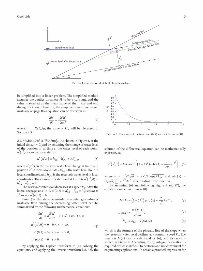
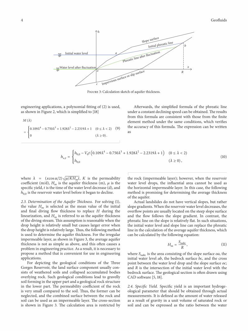
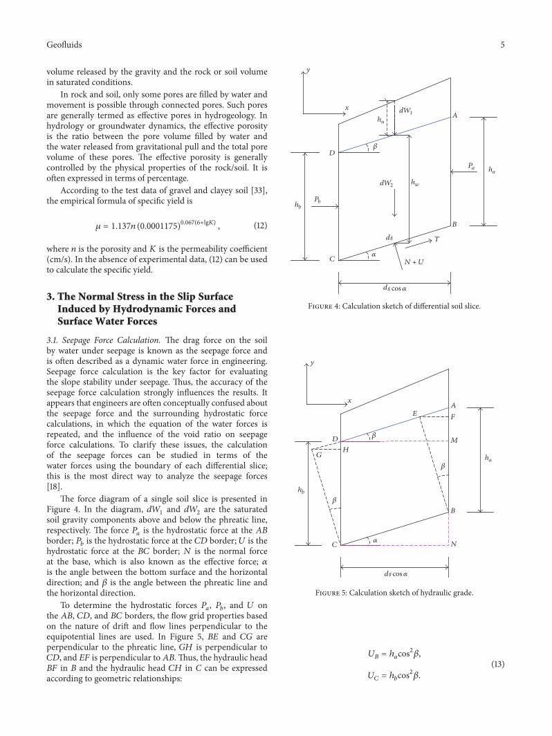
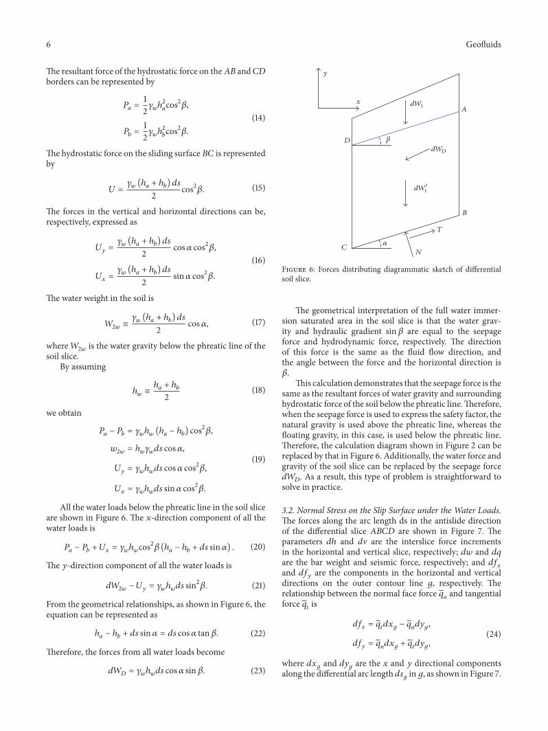
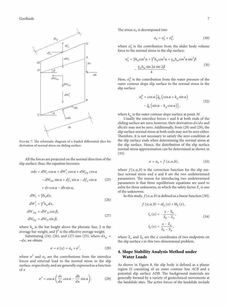
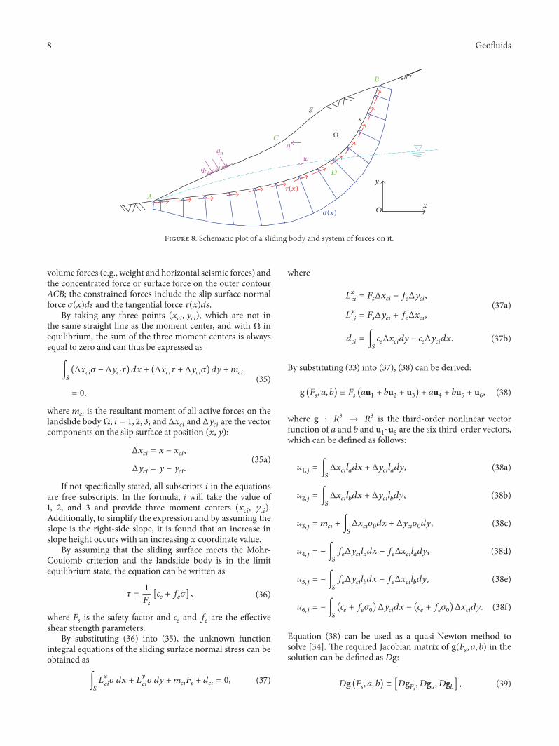
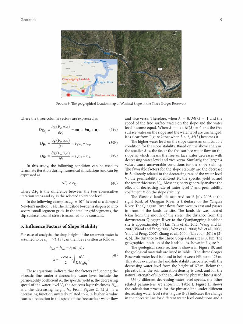
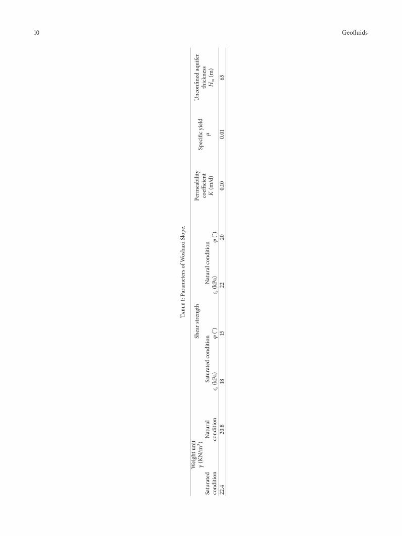
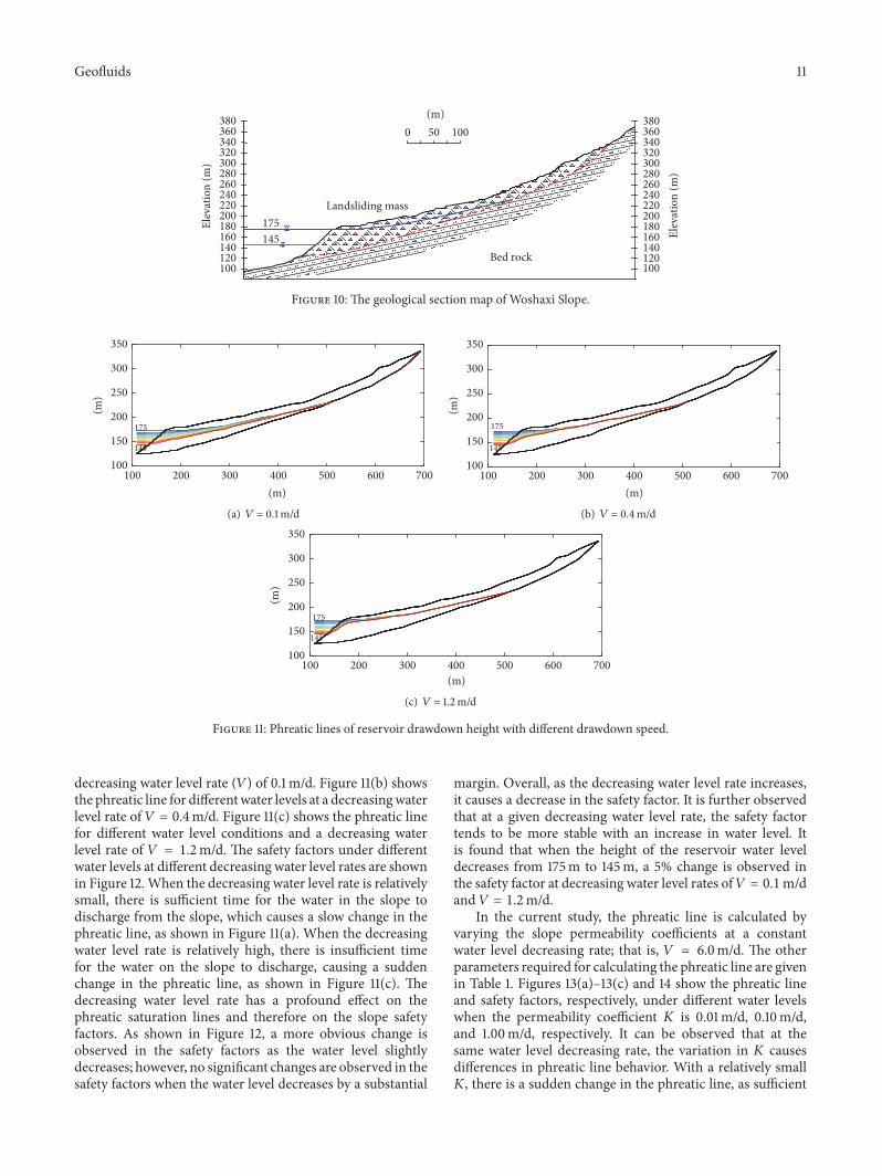
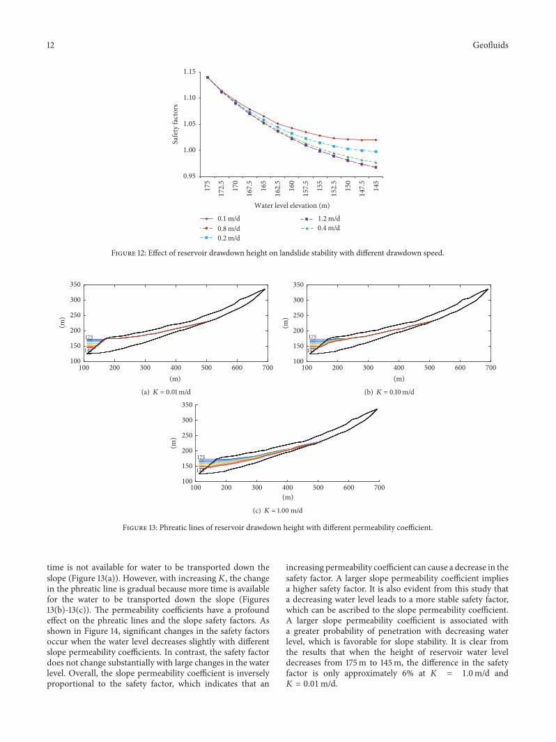
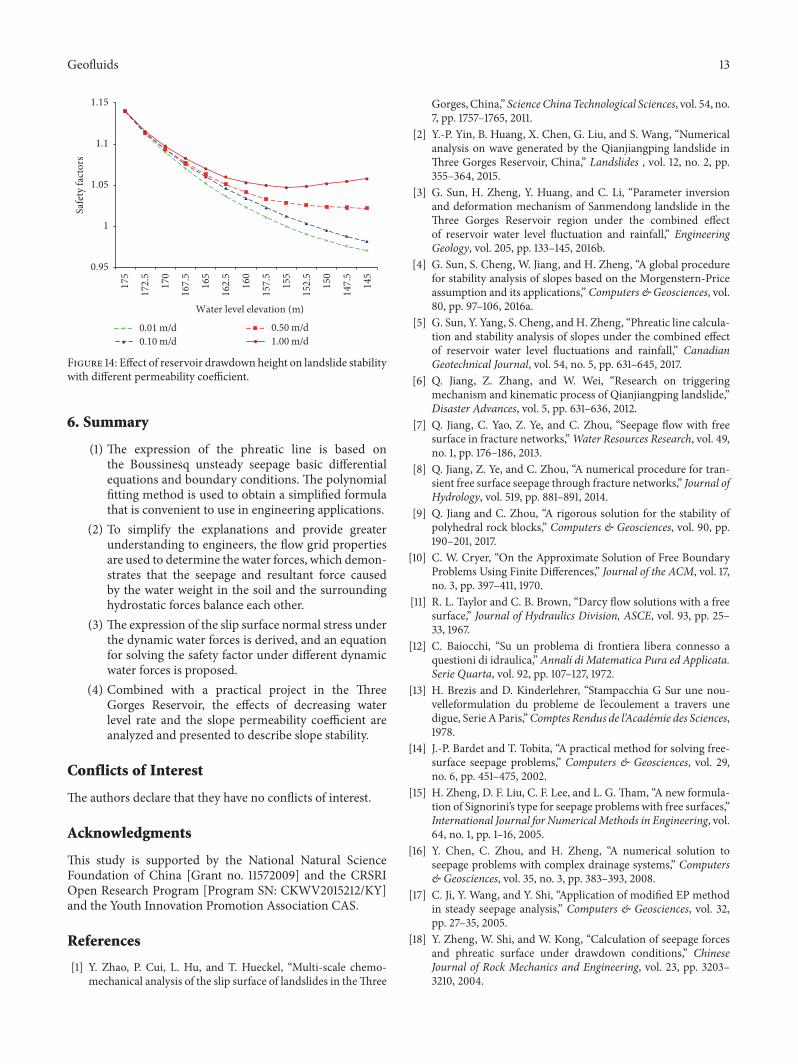
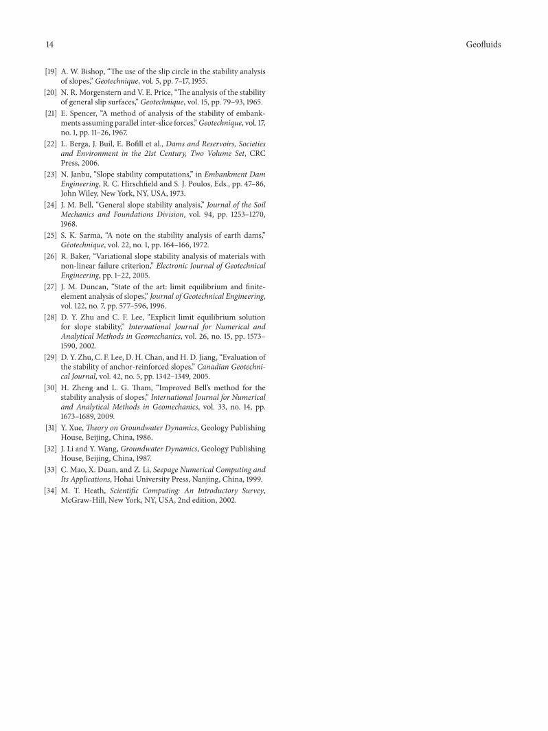

Hindawiwwwhindawicom Volume 2018
Journal of
ChemistryArchaeaHindawiwwwhindawicom Volume 2018
Marine BiologyJournal of
Hindawiwwwhindawicom Volume 2018
BiodiversityInternational Journal of
Hindawiwwwhindawicom Volume 2018
EcologyInternational Journal of
Hindawiwwwhindawicom Volume 2018
Hindawiwwwhindawicom
Applied ampEnvironmentalSoil Science
Volume 2018
Forestry ResearchInternational Journal of
Hindawiwwwhindawicom Volume 2018
Hindawiwwwhindawicom Volume 2018
International Journal of
Geophysics
Environmental and Public Health
Journal of
Hindawiwwwhindawicom Volume 2018
Hindawiwwwhindawicom Volume 2018
International Journal of
Microbiology
Hindawiwwwhindawicom Volume 2018
Public Health Advances in
AgricultureAdvances in
Hindawiwwwhindawicom Volume 2018
Agronomy
Hindawiwwwhindawicom Volume 2018
International Journal of
Hindawiwwwhindawicom Volume 2018
MeteorologyAdvances in
Hindawi Publishing Corporation httpwwwhindawicom Volume 2013Hindawiwwwhindawicom
The Scientific World Journal
Volume 2018Hindawiwwwhindawicom Volume 2018
ChemistryAdvances in
ScienticaHindawiwwwhindawicom Volume 2018
Hindawiwwwhindawicom Volume 2018
Geological ResearchJournal of
Analytical ChemistryInternational Journal of
Hindawiwwwhindawicom Volume 2018
Submit your manuscripts atwwwhindawicom