A Simplified Computer Vision System for Road Surface Inspection and Maintenance

Marcos Quintana, Juan Torres, and José Manuel Menéndez

Abstract—This paper presents a computer vision system whose aim is to detect and classify cracks on road surfaces. Most of the previous works consisted of complex and expensive acquisition systems, whereas we have developed a simpler one composed by a single camera mounted on a light truck and no additional illumination. The system also includes tracking devices in order to geolocalize the captured images. The computer vision algorithm has three steps: hard shoulder detection, cell candidate proposal, and crack classification. First the region of interest (ROI) is de­limited using the Hough transform (HT) to detect the hard shoul­ders. The cell candidate step is divided into two substeps: Hough transform features (HTF) and local binary pattern (LBP). Both of them split up the image into nonoverlapping small grid cells and also extract edge orientation and texture features, respectively. At the fusion stage, the detection is completed by mixing those techniques and obtaining the crack seeds. Afterward, their shape is improved using a new developed morphology operator. Finally, one classification based on the orientation of the detected lines has been applied following the Chain code. Massive experiments were performed on several stretches on a Spanish road showing very good performance.

Index Terms—Road safety, computer vision, pattern recogni­tion, image processing.

I. INTRODUCTION

T HE maintenance of roads is a critical problem to improve their sustainability and the security of the vehicles. Road

sections that contain a high density of cracks should be periodi­cally reviewed in order to avoid problems in the future. Their detection is critical, especially concerning some problematic cracks. Crack type, severity and size are important criteria to maintain and repair roads. Pavement distress refers to the visible imperfection of the pavement surface. Often the distress is noticeably expressed by various types of cracks at the surface.

Crack detection and classification in road surface analysis have experienced a great development over the last decades. These tasks are traditionally done by human experts using visual inspection along the monitored road. Nowadays, imaging technologies are chosen for many transportation applications, including automatic inspection and monitoring. That increasing

demand is partly driven by the evolution of imaging technolo­gies, especially regarding optics and sensors.

For crack detection we follow the definitions of PIARC [4]: 1) a crack has at least 0, 15 m of length and 1 mm of width; 2) a crack is longitudinal if its orientation is 1:3 minimum (1 parallel and 3 perpendicular to the road axis); otherwise it is considered as transversal; 3) Alligator cracks are those that form a grid having 3 pieces minimum in each direction, and the diameter of each piece is less than 300 mm; if the diameter is higher, the crack is classified as block type. The first two are just based on the orientation of the crack whereas the last two also take into account the crack density.

One of the greatest challenges for computer vision algorithms is the variability of the lighting conditions. Systems that require a high percentage of relevant instances retrieved, like the one presented here, usually include lighting devices to assure the appropriate illumination of the surfaces. Vehicles including a complex and expensive equipment like [29] or [30] have been de­veloped in the last years with commercial purposes. Both of them include a complex lighting system, relying on the coherence of different laser devices. They use linear cameras to capture the surface of the road, like the vehicle presented in Section III.

Nevertheless, the required lighting devices used for illumi­nating the field of view are expensive, and the daylight hours were enough in previous campaigns to capture the affected roads. In this paper, a simple-but-effective low cost computer vision in-vehicle system, able to detect and classify cracks in roads, is explained. The system works with no additional source of light apart from the Sun. This work demonstrates that weather conditions in some countries such as Spain, enable to achieve good results in tasks related to crack detection and classification without a great investment. The target of the system is offering a new method to evaluate the state of the roads under daylight illumination conditions.

A summary of the computer vision system is shown in Fig. 1. It included two phases: acquisition and analysis. The first one includes image acquisition and geo-localization data. The analysis step, performed offline, includes the Region Of Interest (ROI) delimitation, crack detection and classification.

The rest of the paper is organized as follows: Section II intro­duces the current state of the art of previous published systems. In Section III the components of the system and how they work together are detailed. Our approach to detect and classify cracks is explained in Section IV. Section V includes the specification of the tests performed. Section VI shows the results obtained in the different tests in order to validate the system performance. Finally, the conclusions and future research lines extracted from this work are discussed in Section VII.

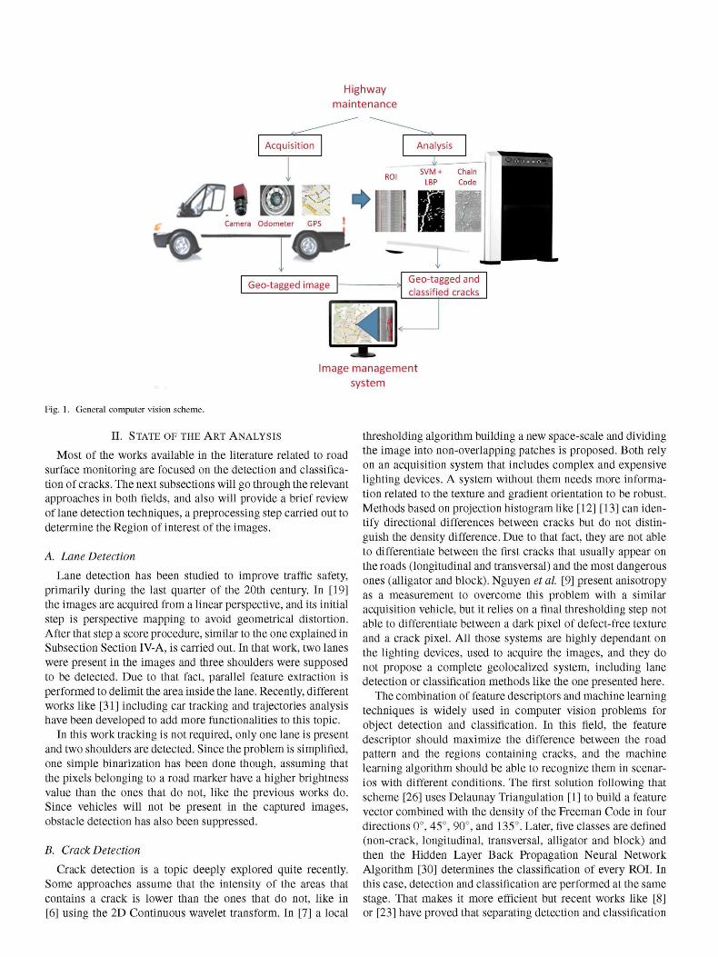
Highway

maintenance

Acquisition Analysis

Camera Odometer GPS

ROI SVM+ Chain

LBP Code

Geo-tagged ¡mage Geo-tagged and classified cracks

Image management

system

Fig. 1. General computer vision scheme.

II. STATE OF THE ART ANALYSIS

Most of the works available in the literature related to road surface monitoring are focused on the detection and classifica­tion of cracks. The next subsections will go through the relevant approaches in both fields, and also will provide a brief review of lane detection techniques, a preprocessing step carried out to determine the Region of interest of the images.

A. Lane Detection

Lane detection has been studied to improve traffic safety, primarily during the last quarter of the 20th century. In [19] the images are acquired from a linear perspective, and its initial step is perspective mapping to avoid geometrical distortion. After that step a score procedure, similar to the one explained in Subsection Section IV-A, is carried out. In that work, two lanes were present in the images and three shoulders were supposed to be detected. Due to that fact, parallel feature extraction is performed to delimit the area inside the lane. Recently, different works like [31] including car tracking and trajectories analysis have been developed to add more functionalities to this topic.

In this work tracking is not required, only one lane is present and two shoulders are detected. Since the problem is simplified, one simple binarization has been done though, assuming that the pixels belonging to a road marker have a higher brightness value than the ones that do not, like the previous works do. Since vehicles will not be present in the captured images, obstacle detection has also been suppressed.

B. Crack Detection

Crack detection is a topic deeply explored quite recently. Some approaches assume that the intensity of the areas that contains a crack is lower than the ones that do not, like in [6] using the 2D Continuous wavelet transform. In [7] a local

thresholding algorithm building a new space-scale and dividing the image into non-overlapping patches is proposed. Both rely on an acquisition system that includes complex and expensive lighting devices. A system without them needs more informa­tion related to the texture and gradient orientation to be robust. Methods based on projection histogram like [12] [13] can iden­tify directional differences between cracks but do not distin­guish the density difference. Due to that fact, they are not able to differentiate between the first cracks that usually appear on the roads (longitudinal and transversal) and the most dangerous ones (alligator and block). Nguyen et al. [9] present anisotropy as a measurement to overcome this problem with a similar acquisition vehicle, but it relies on a final thresholding step not able to differentiate between a dark pixel of defect-free texture and a crack pixel. All those systems are highly dependant on the lighting devices, used to acquire the images, and they do not propose a complete geolocalized system, including lane detection or classification methods like the one presented here.

The combination of feature descriptors and machine learning techniques is widely used in computer vision problems for object detection and classification. In this field, the feature descriptor should maximize the difference between the road pattern and the regions containing cracks, and the machine learning algorithm should be able to recognize them in scenar­ios with different conditions. The first solution following that scheme [26] uses Delaunay Triangulation [1] to build a feature vector combined with the density of the Freeman Code in four directions 0°, 45°, 90°, and 135°. Later, five classes are defined (non-crack, longitudinal, transversal, alligator and block) and then the Hidden Layer Back Propagation Neural Network Algorithm [30] determines the classification of every ROI. In this case, detection and classification are performed at the same stage. That makes it more efficient but recent works like [8] or [23] have proved that separating detection and classification

produces an important improvement in the efficacy of the algo­rithm, specially important in applications that require a high re­call, like this work. The former [23] includes an extensive study on the road materials and how they can get damaged. Based on that study, a multiclass Support Vector Machine (SVM) is implemented to parameterize the different weights and thresholds of the algorithm according to the nature of the pave­ment. It proposes a feature descriptor trying to exploit the texture features of the road, but it does not take into account the geometrical features of the detected cracks in order to classify the cracks and evaluate the damage of the road. In addition, the acquisition vehicle includes a very complex lighting system, however it does not propose any geo-localization method.

The solution proposed in [8] relies on the following crack description:

1) There is a considerable intensity contrast between the pixels that belong to a crack and those that do not.

2) The cracks are composed by a sum of lines. 3) The changes in the intensity around the two sides of

cracks can be considered as symmetric.

To express them in a feature vector, first the gradient is calculated in four orientations and then the Hough Transform (HT) [21] is applied to detect lines (cracks are composed by their composition). Finally a rotation invariant feature vector is obtained. After that, a SVM (previously trained) estimates the probability of every cell to contain or not a crack. The results of this proposal could be more robust by adding a more precise training step, able to characterize cracks on all feasible conditions that could be found in the different types of roads. In addition, this work is mainly focused on detection, and does not include any method to classify cracks.

Following the previous scheme, there are many methods based on the properties of the background (the road). Most of the roads can be characterized by a particular texture pattern. In [11] a multiresolution pyramid is built using morphologi­cal operators. Then the Co-Occurrence matrix and one local threshold are computed for every scale. This solution is highly dependant on the set of pairs chosen to build the Co-Occurrence matrix. In [23] Local Binary Pattern is combined with other techniques to classify the road pavement. A solution mostly based on that procedure is presented in [25]. In this case, the image is divided in ROIs and depending on the intensity values of its neighborhood, a binary pattern is built. The shape of that pattern is studied to determine which class each patch belongs to. But that solution is not able by itself, to define accurately the lines that compose the detected cracks.

Since local thresholding techniques are not robust enough for the acquisition proposed in this work, a fusion of the other two groups of techniques is considered the most reliable solution. For that aim, first points likely to belong to a crack feature are extracted using a feature descriptor and a machine learning algorithm on one side, and background modelization based on texture properties on the other. A statistical solution based on the distribution obtained with both of them should be chosen to improve previous results in this field. Mean-variance [27] is the most desirable solution, and an implemented evolution of this method will be further explained in Section IV.

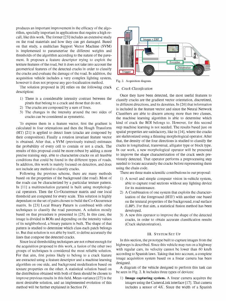
Fig. 2. Acquisition diagram.

C. Crack Classification

Once they have been detected, the most useful features to classify cracks are the gradient vector orientation, discretized, in different directions, and its densities. In [26] that information is included in the feature vector and since the Neural Network Classifiers are able to discern among more than two classes, the machine learning algorithm is able to determine which kind of crack the ROI belongs to. However, for this second step machine learning is not needed. The results based just on spatial properties are satisfactory, like in [14], where the cracks are skeletonized using a thinning morphological operator. After that, the density of the four directions is studied to classify the cracks in longitudinal, transversal, alligator type or block type. In our work, a new morphological operator will be presented to improve the shape characterization of the crack seeds pre­viously detected. That operator performs a preprocessing step needed to locate accurately the cracks before representing them using the chain code.

There are three main scientific contributions in our proposal:

1) A novel and simple computer vision in-vehicle system, able to capture road sections without any lighting device for its maintenance.

2) A Combination of one system that exploits the character­ization of the foreground (HTF) with another one based on the textural properties of the background, road surface (LBP). For that aim, a statistical fusion method has been developed.

3) A new thin operator to improve the shape of the detected cracks, in order to obtain accurate classification results (Crack skeletonization).

III. SYSTEM SET U P

In this section, the prototype built to capture images from the highways is described. Since this vehicle may run on a highway with regular cars, its velocity cannot be lower than 60 km/h according to Spanish laws. Taking that into account, a complete image acquisition system based on a linear camera has been designed.

A diagram of the vehicle designed to perform this task can be seen in Fig. 2. It includes three types of devices:

1) Image capturing system. A linear camera acquires the images using the CameraLink interface [17]. That camera includes a sensor of 4K. Since the width of a Spanish

<Crack> <Situat¡on/> <Type/> <Length/> <Area/>

</Crack>

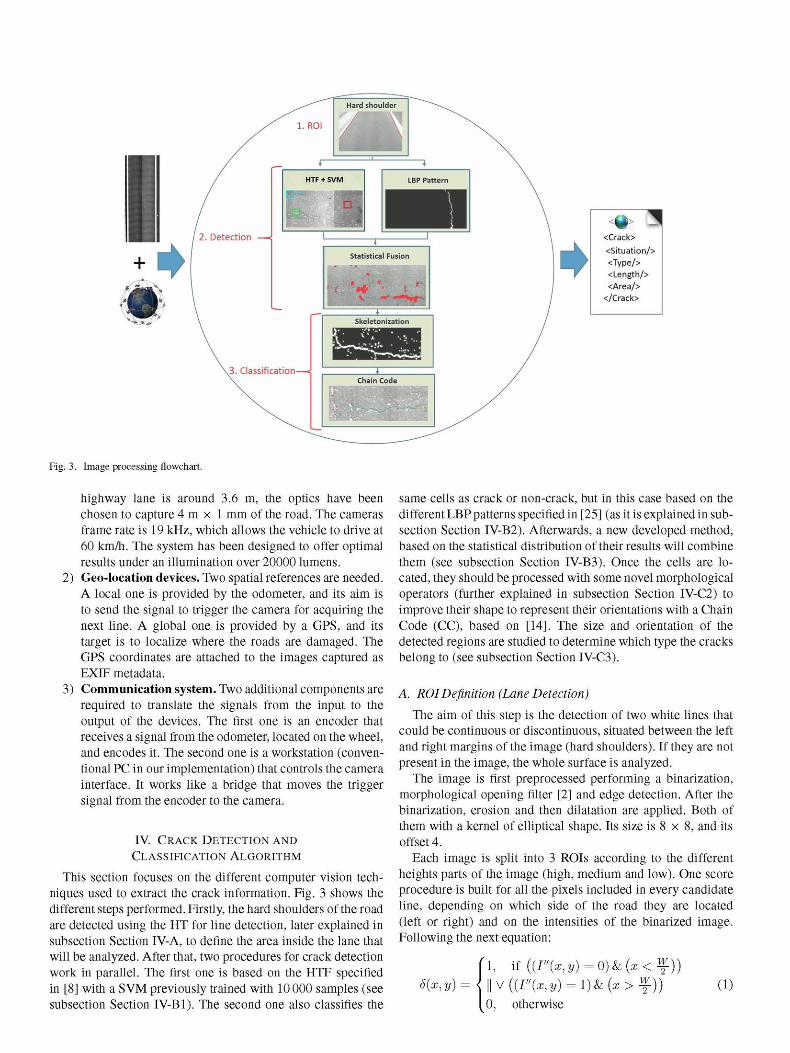
Fig. 3. Image processing flowchart.

highway lane is around 3.6 m, the optics have been chosen to capture 4 m x 1 mm of the road. The cameras frame rate is 19 kHz, which allows the vehicle to drive at 60 km/h. The system has been designed to offer optimal results under an illumination over 20000 lumens.

2) Geo-location devices. Two spatial references are needed. A local one is provided by the odometer, and its aim is to send the signal to trigger the camera for acquiring the next line. A global one is provided by a GPS, and its target is to localize where the roads are damaged. The GPS coordinates are attached to the images captured as EXIF metadata.

3) Communication system. Two additional components are required to translate the signals from the input to the output of the devices. The first one is an encoder that receives a signal from the odometer, located on the wheel, and encodes it. The second one is a workstation (conven­tional PC in our implementation) that controls the camera interface. It works like a bridge that moves the trigger signal from the encoder to the camera.

IV. CRACK DETECTION AND

CLASSIFICATION ALGORITHM

This section focuses on the different computer vision tech­niques used to extract the crack information. Fig. 3 shows the different steps performed. Firstly, the hard shoulders of the road are detected using the HT for line detection, later explained in subsection Section IV-A, to define the area inside the lane that will be analyzed. After that, two procedures for crack detection work in parallel. The first one is based on the HTF specified in [8] with a SVM previously trained with 10 000 samples (see subsection Section IV-B1). The second one also classifies the

same cells as crack or non-crack, but in this case based on the different LBP patterns specified in [25] (as it is explained in sub­section Section IV-B2). Afterwards, a new developed method, based on the statistical distribution of their results will combine them (see subsection Section IV-B3). Once the cells are lo­cated, they should be processed with some novel morphological operators (further explained in subsection Section IV-C2) to improve their shape to represent their orientations with a Chain Code (CC), based on [14]. The size and orientation of the detected regions are studied to determine which type the cracks belong to (see subsection Section IV-C3).

A. ROI Definition (Lane Detection)

The aim of this step is the detection of two white lines that could be continuous or discontinuous, situated between the left and right margins of the image (hard shoulders). If they are not present in the image, the whole surface is analyzed.

The image is first preprocessed performing a binarization, morphological opening filter [2] and edge detection. After the binarization, erosion and then dilatation are applied. Both of them with a kernel of elliptical shape. Its size is 8 x 8, and its offset 4.

Each image is split into 3 ROIs according to the different heights parts of the image (high, medium and low). One score procedure is built for all the pixels included in every candidate line, depending on which side of the road they are located (left or right) and on the intensities of the binarized image. Following the next equation:

1, if ((/"(*, y) = 0 ) & ( z < f ) ) d(x,y) = {\\V ((I"(x,y) = l)&z(x > f))

0, otherwise (1)

where: where:

1) / " is the binarized image after applying morphological operators.

2) W is the width of the image. 3) A is the logical operator AND. 4) V is the logical operator OR. 5) 6(x, y) is the score for every pixel.

The line whose pixels have the highest score will define the ROI boundary for the given image. The expression shown for the scoring procedure has been designed to define the hard shoulder on the left side of the image. The equation works as well for the right side of the image, just swapping 0 and 1. Finally two equations will define the margins of the ROI:

a,iX + hy + Ci = 0 (2)

where i G {'Left'/Right'}.

B. Crack Candidates

Once the ROI is defined, the algorithm will detect those pixels with a high probability of being located inside a crack. The first selected solution is based on the foreground properties (cracks) [8]. The second one is based on the background proper­ties (road pattern). Both of them will be joint in the fusion step developed for this system. That novel method is based on the statistical properties of the distribution obtained after applying the algorithms.

1) HTF Extraction and Machine Learning: This module splits up the image in non-overlapping small grid cells. In this work the size is set to 17 x 17 pixels, as justified later on. The first step is to extract the gradient in 4 different directions {x+, x~, y+, y~} for all the cells included in the ROI. The next equation shows the calculation for x+:

Gx+{x,y) I(x+ l,y) -I(x,y))

(3)

where I is the original image. Later, the HT is applied to the 4 images obtained from the

edge responses. The results will be quantized in an histogram with m bins for p, and n for 9. Four matrices are built (one for every direction) with the histograms values. Every one of them has a size of m x n. The values for p are calculated with the following equation for every bin of 6:

Pxy = (v ' cos(#m)) + (x • (sin(0m)) (4)

where:

1) ie { 0 , . . . , n - l } . 2) 6m is the mean value of 6 for every bin.

Since the histograms obtained can be considered as disperse, concentricity measurements are used to obtain more representa­tive values. For each bin with a different value of 6 (we assume that the summation of bins for each 9 is constant), the maximal concentricity measurement of r on that angle is stored.

1) r is the concentricity measurement vector. 2) ¿ € { 0 , . . . , n } . 3) j e { 0 , . . . , m } .

To be rotation invariant, we sort the r concentricity measures, and form an m elements vector v for every H. The measures with the largest p' and 6' concentricity are used as the main directions to calculate HTF, following the next equation:

maxCon(yO, #) = max(V+) • \ . ((w+(* + 1) — w+(*)) ' al) ¿=o

n

+ m a x ( V _ ) - ^ ((<;_(«+!) -v-(i)) -a1) (6) ¿=o

where:

1) v+ and v_ are the p concentricity measure vectors for all the values of 6 included in H+ and H- Hough matrices.

2) max(«±) indicates the largest p concentricity. 3) a is an empirically chosen attenuation factor (in our

implementation, we set it as 0.9). 4) i G 0..n - 1.

From now on just the Hough matrices of the main direction will be used to continue with the different calculations. In the end, a feature vector with the following elements has been obtained for every non-overlapping cell included in the ROI:

I The summation of H±'s column. Which measures the total strength of gradient responses.

FV[O] = Y^H[DDir-2][(j-0)] (7) ¿=o

n

FV[l] = Y.H KDDtr • 2) + !] 1(3 • binse)] (8) ¿=o

where: a) n e (O..,obins - 1). b) H Is an array containing the results for the Hough

Transform in four different directions. c) binse is the number of bins for 9. d) DDir is the dominant direction (+ or - ) based on the

concentricity measurements G (0, 1).

II The largest r concentricity. Defined as:

FV[2] = max(y+) + max(Vl). (9)

III The angle concentricity. Defined as:

FV[i + 2] =AC[i] = max(V+)

, ((v-(i+l)-v-(i))

r[i] = irmxConc(9[i][j]) (5)

max (VI)

where i e l . . r a - l (Number of 0 bins —1).

(10)

IV The difference in the measurements of '+' and '—' values. Defined as:

Support Vector Machine learning curve with HTF features

FV[m + 2] = Diff(v+,v-)

where || || is the g\ norm operator;

\v+ +V-

FV\ 3] =

± are the original vectors of v± before sorting;

FV[m + 4] = fr(G+,G.

(11)

(12)

(13)

where:

a) G± are the positive and negative values after the gradient operator of the original cell.

b) Equations (11) and (12) indicate the overall difference of the + and - channels for the p concentricity.

c) Equation (11) represents the correlation function of G+ and G—, and measures the inconsistency of shifts between the + and - gradient values.

d) Usually a crack cell has a high correlation between G+ and G_. For non-crack cells, the shifts are usually inconsistent. In our implementation m and n have been set to 24 and 15 respectively.

The implemented SVM has been trained with 10 000 pairs of positive and negative cells of 17 x 17 pixels. They have been classified determining which regions belong to a crack and which do not. The samples have been chosen in order to build a set that covers all the possible environmental conditions. Those cells far from the decision boundaries have been discarded. Dif­ferent values of the following properties have been combined for that aim:

(a) Pavement types. Following the specification in [23]. (b) Road age. From 5 to 50 years. (c) Road damage, from brand-new roads to roads with high

distress.

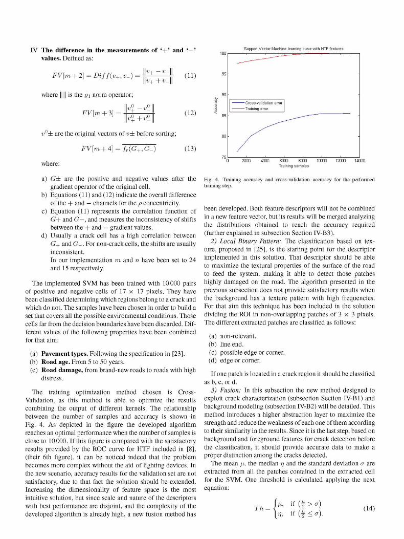
The training optimization method chosen is Cross-Validation, as this method is able to optimize the results combining the output of different kernels. The relationship between the number of samples and accuracy is shown in Fig. 4. As depicted in the figure the developed algorithm reaches an optimal performance when the number of samples is close to 10000. If this figure is compared with the satisfactory results provided by the ROC curve for HTF included in [8], (their 6th figure), it can be noticed indeed that the problem becomes more complex without the aid of lighting devices. In the new scenario, accuracy results for the validation set are not satisfactory, due to that fact the solution should be extended. Increasing the dimensionality of feature space is the most intuitive solution, but since scale and nature of the descriptors with best performance are disjoint, and the complexity of the developed algorithm is already high, a new fusion method has

•-i'-,

90

- ... .

1 1 1 1 1 1

2000 4000 6000 8000 Training samples

10000 12000 14000

Fig. 4. Training accuracy and cross-validation accuracy for the performed training step.

been developed. Both feature descriptors will not be combined in a new feature vector, but its results will be merged analyzing the distributions obtained to reach the accuracy required (further explained in subsection Section IV-B3).

2) Local Binary Pattern: The classification based on tex­ture, proposed in [25], is the starting point for the descriptor implemented in this solution. That descriptor should be able to maximize the textural properties of the surface of the road to feed the system, making it able to detect those patches highly damaged on the road. The algorithm presented in the previous subsection does not provide satisfactory results when the background has a texture pattern with high frequencies. For that aim this technique has been included in the solution dividing the ROI in non-overlapping patches of 3 x 3 pixels. The different extracted patches are classified as follows:

(a) non-relevant. (b) line end. (c) possible edge or corner. (d) edge or corner.

If one patch is located in a crack region it should be classified as b, c, or d.

3) Fusion: In this subsection the new method designed to exploit crack characterization (subsection Section IV-Bl) and background modeling (subsection IV-B2) will be detailed. This method introduces a higher abstraction layer to maximize the strength and reduce the weakness of each one of them according to their similarity in the results. Since it is the last step, based on background and foreground features for crack detection before the classification, it should provide accurate data to make a proper distinction among the cracks detected.

The mean p, the median r¡ and the standard deviation a are extracted from all the patches contained in the extracted cell for the SVM. One threshold is calculated applying the next equation:

Th = M, if (f > a)

V, i f ( f < a ) . (14)

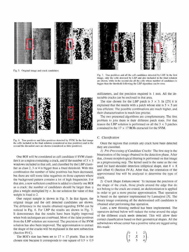
Fig. 5. Original image and crack candidates.

Fig. 6. True positives and false positives detected by SVM. In the first image the cells included in the final solution (considered as true positives) and in the second the discarded ones are shown (considered as false positives).

One ROI will be considered as cell candidate if SVM classi­fies it as a region containing a crack, and if the number of 3 x 3 windows included in that cell, and classified by the LBP classi­fier as class 2, 3 or 4 is bigger than a fixed threshold. With this combination the number of false positives has been decreased, but there are still some false negatives on those captures where the background pattern contains a lot of high frequencies. For that aim, a new sufficient condition is added to classify one ROI as a crack: the number of candidates should be larger than r\ plus a weight multiplied by a. In our solution the value of that weight is fixed to 2.

One output sample is shown in Fig. 5. In that figure, the original image and the cell detected candidates are shown. The difference in the results obtained regarding SVM can be noticed in Fig. 6. For LBP the results are shown in Fig. 7. It demonstrates that the results have been highly improved when both techniques are combined. Most of the false positives from the LBP solution are removed. The precision of the SVM solution has also been improved. The approximation to extract the shape of the cracks will be explained in the next subsection (Section IV-C).

The ROFs size has been set to 17 x 17 pixels. That is the chosen size because it corresponds to one square of 0.9 x 0.9

Fig. 7. True positives and all the cell candidates detected by LBP. In the first image, only the cells detected by LBP and also included in the final solution are shown, while in the second one all the cells whose number of candidates is bigger than the threshold following the LBP algorithm can be seen.

millimeters, and the precision required is 1 mm. All the de­tectable cracks can be enclosed in that area.

The size chosen for the LBP patch is 3 x 3. In [25] it is explained that the results with a patch whose size is 5 x 5 are less efficient: The possible combinations are much higher, and their characterization is much less precise.

The two presented algorithms are complementary. The first problem to join them is their different patch sizes. For that reason the LBP solution is performed on all the 3 x 3 patches contained in the 17 x 17 ROIs extracted for the SVM.

C. Classification

Once the regions that contain any crack have been detected they are classified.

1) Pre-Processing of Candidate Cracks: The first step is the binarization of the image obtained in the detection phase. After that, closure morphological filtering is performed on that image as a preprocessing step. The kernel used is the same as the one used for hard shoulder detection (elliptical shape, size 8 x 8 and offset 4) (Section IV-A). After that, the orientation of the approximated line will be analyzed to determine the type of crack.

2) Crack Shape Enhancement: To increase the precision of the shape of the crack, those pixels around the edge that do not belong to the crack are erased, an skeletonization is applied in order to get a more precise approximation. That operation is based on the operator implemented by Lantuejoul [5]. The binary image containing all the skeletonized cell candidates is obtained after performing that operation.

Later, a new thinning method has been implemented. The operators defined below will reduce the noise around the edge of the different crack seeds detected. This will allow their correct classification based on their geometrical shapes. All the subwindows whose center has a positive value are tagged using this mask:

(° * 2\ 7 X 3 . \ 6 5 A)

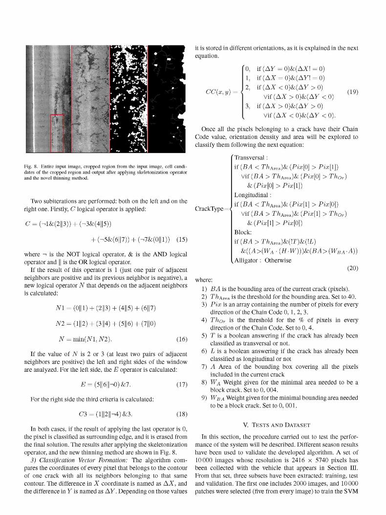
Fig. 8. Entire input image, cropped region from the input image, cell candi­dates of the cropped region and output after applying skeletonization operator and the novel thinning method.

Two subiterations are performed: both on the left and on the right one. Firstly, C logical operator is applied:

C=H&(2||3)) + h3&(4||5))

+ (-5&(6||7)) + (-7&(0||l)) (15)

where -• is the NOT logical operator, & is the AND logical operator and || is the OR logical operator.

If the result of this operator is 1 (just one pair of adjacent neighbors are positive and its previous neighbor is negative), a new logical operator N that depends on the adjacent neighbors is calculated:

N\ |1) + (2||3) + (4||5) + (6||7)

AT2=(1||2) + (3||4) + (5||6) + (7||0)

Ar = min(Ari,AT2). (16)

If the value of N is 2 or 3 (at least two pairs of adjacent neighbors are positive) the left and right sides of the window are analyzed. For the left side, the E operator is calculated:

£7=(5||6||-.0)&7. (17)

For the right side the third criteria is calculated:

C3 = (l | |2 |h4)&3. (18)

In both cases, if the result of applying the last operator is 0, the pixel is classified as surrounding edge, and it is erased from the final solution. The results after applying the skeletonization operator, and the new thinning method are shown in Fig. 8.

3) Classification Vector Formation: The algorithm com­pares the coordinates of every pixel that belongs to the contour of one crack with all its neighbors belonging to that same contour. The difference in X coordinate is named as AX, and the difference in Y is named as A y . Depending on those values

CC(x,y) (19)

CrackType=<

it is stored in different orientations, as it is explained in the next equation.

'0, if (Ay = 0)&(AX! = 0)

1, if(AX = 0)&(Ay! = 0)

2, i f ( A X < 0 ) & ( A y >0 )

vif(Ax >o)&(Ay <o) 3, if (AX > 0)&(Ay >0 )

vif(Ax <o)&(Ay <o).

Once all the pixels belonging to a crack have their Chain Code value, orientation density and area will be explored to classify them following the next equation:

Transversal:

if {BA < T/lArea)& {Pix[0\ > Pix[l\)

Vif {BA > T/lArea)& {Pix[0\ > Th0r)

& [Pix[0] > Pix[l\)

Longitudinal:

if {BA < T/lArea)& [Pix[i] > Pix[0])

Vif {BA > T/lArea)& {Pix[l\ > Th0r)

& {Pix[l\ > Pix[0])

Block:

if{BA>ThAiea)&i{\T)&i{\L)

¡k{{A>{WA • {H-W)))¡k{BA>{WBA-A))

Alligator : Otherwise (20)

where: 1) BA is the bounding area of the current crack (pixels). 2) T/iArea is the threshold for the bounding area. Set to 40. 3) Pix is an array containing the number of pixels for every

direction of the Chain Code 0, 1, 2, 3. 4) Thor is the threshold for the % of pixels in every

direction of the Chain Code. Set to 0, 4. 5) T is a boolean answering if the crack has already been

classified as transversal or not. 6) L is a boolean answering if the crack has already been

classified as longitudinal or not 7) A Area of the bounding box covering all the pixels

included in the current crack 8) WA Weight given for the minimal area needed to be a

block crack. Set to 0, 004. 9) WB A Weight given for the minimal bounding area needed

to be a block crack. Set to 0, 001.

V. TESTS AND DATASET

In this section, the procedure carried out to test the perfor­mance of the system will be described. Different season results have been used to validate the developed algorithm. A set of 10 000 images whose resolution is 2416 x 5740 pixels has been collected with the vehicle that appears in Section III. From that set, three subsets have been extracted: training, test and validation. The first one includes 2000 images, and 10000 patches were selected (five from every image) to train the SVM

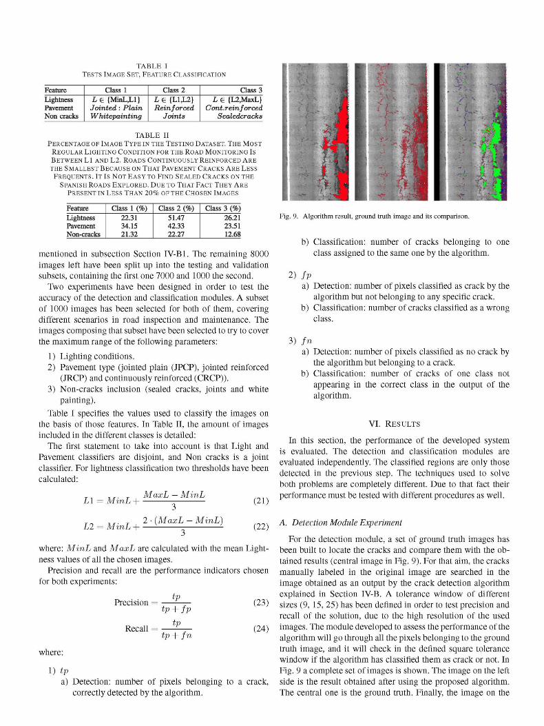
TABLE I TESTS IMAGE SET, FEATURE CLASSIFICATION

Feature Lightness Pavement Non cracks

Class 1 L £ {MinL,Ll) Jointed : Plain Whitepainting

Class 2 L e {L1,L2} Reinforced

Joints

Class 3 L e {L2,MaxL}

Cont.rein forced Sealedcracks

TABLE II PERCENTAGE OF IMAGE TYPE IN THE TESTING DATASET. THE MOST

REGULAR LIGHTING CONDITION FOR THE ROAD MONITORING IS BETWEEN L1 AND L2. ROADS CONTINUOUSLY REINFORCED ARE THE SMALLEST BECAUSE ON THAT PAVEMENT CRACKS ARE LESS

FREQUENTS. IT IS NOT EASY TO FIND SEALED CRACKS ON THE SPANISH ROADS EXPLORED. DUE TO THAT FACT THEY ARE

PRESENT IN LESS THAN 20% OF THE CHOSEN IMAGES

Feature Lightness Pavement Non-cracks

Class 1 (%) 22.31 34.15 21.32

Class 2 (%) 51.47 42.33 22.27

Class 3 (%) 26.21 23.51 12.68

mentioned in subsection Section IV-B1. The remaining 8000 images left have been split up into the testing and validation subsets, containing the first one 7000 and 1000 the second.

Two experiments have been designed in order to test the accuracy of the detection and classification modules. A subset of 1000 images has been selected for both of them, covering different scenarios in road inspection and maintenance. The images composing that subset have been selected to try to cover the maximum range of the following parameters:

1) Lighting conditions. 2) Pavement type (jointed plain (JPCP), jointed reinforced

(JRCP) and continuously reinforced (CRCP)). 3) Non-cracks inclusion (sealed cracks, joints and white

painting).

Table I specifies the values used to classify the images on the basis of those features. In Table II, the amount of images included in the different classes is detailed:

The first statement to take into account is that Light and Pavement classifiers are disjoint, and Non cracks is a joint classifier. For lightness classification two thresholds have been calculated:

LI = MinL-

L2 = MinL +

MaxL - Mini

3 2 • (MaxL - MinL)

3

(21)

(22)

where: MinL and MaxL are calculated with the mean Light­ness values of all the chosen images.

Precision and recall are the performance indicators chosen for both experiments:

tp Precision =

Recall =

tp + fp tp

tp + fn

(23)

(24)

where:

1) tp a) Detection: number of pixels belonging to a crack,

correctly detected by the algorithm.

Fig. 9. Algorithm result, ground truth image and its comparison.

b) Classification: number of cracks belonging to one class assigned to the same one by the algorithm.

2) fP

a) Detection: number of pixels classified as crack by the algorithm but not belonging to any specific crack.

b) Classification: number of cracks classified as a wrong class.

3) fn a) Detection: number of pixels classified as no crack by

the algorithm but belonging to a crack. b) Classification: number of cracks of one class not

appearing in the correct class in the output of the algorithm.

VI. RESULTS

In this section, the performance of the developed system is evaluated. The detection and classification modules are evaluated independently. The classified regions are only those detected in the previous step. The techniques used to solve both problems are completely different. Due to that fact their performance must be tested with different procedures as well.

A. Detection Module Experiment

For the detection module, a set of ground truth images has been built to locate the cracks and compare them with the ob­tained results (central image in Fig. 9). For that aim, the cracks manually labeled in the original image are searched in the image obtained as an output by the crack detection algorithm explained in Section IV-B. A tolerance window of different sizes (9, 15, 25) has been defined in order to test precision and recall of the solution, due to the high resolution of the used images. The module developed to assess the performance of the algorithm will go through all the pixels belonging to the ground truth image, and it will check in the defined square tolerance window if the algorithm has classified them as crack or not. In Fig. 9 a complete set of images is shown. The image on the left side is the result obtained after using the proposed algorithm. The central one is the ground truth. Finally, the image on the

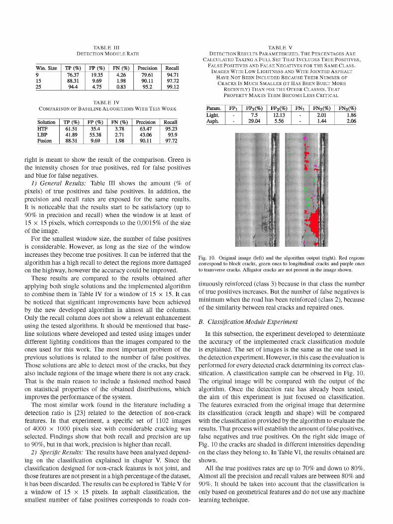
TABLE III DETECTION MODULE RATE

Win. Size 9 15 25

TP(%) 76.37 88.31 944

FP(%) 19.35 9.69 4.75

FN(%) 4.26 1.98 0.83

Precision 79.61 90.11 95.2

Recall 94.71 97.72 99.12

TABLE IV COMPARISON OF BASELINE ALGORITHMS WITH THIS WORK

Solution HTF LBP Fusion

TP(%) 61.51 41.89 88.31

FP(%) 35.4

55.38 9.69

FN(%) 3.78 2.71 1.98

Precision 63.47 43.06 90.11

Recall 95.23 93.9

97.72

right is meant to show the result of the comparison. Green is the intensity chosen for true positives, red for false positives and blue for false negatives.

1) General Results: Table III shows the amount (% of pixels) of true positives and false positives. In addition, the precision and recall rates are exposed for the same results. It is noticeable that the results start to be satisfactory (up to 90% in precision and recall) when the window is at least of 15 x 15 pixels, which corresponds to the 0,0015% of the size of the image.

For the smallest window size, the number of false positives is considerable. However, as long as the size of the window increases they become true positives. It can be inferred that the algorithm has a high recall to detect the regions more damaged on the highway, however the accuracy could be improved.

These results are compared to the results obtained after applying both single solutions and the implemented algorithm to combine them in Table IV for a window of 15 x 15. It can be noticed that significant improvements have been achieved by the new developed algorithm in almost all the columns. Only the recall column does not show a relevant enhancement using the tested algorithms. It should be mentioned that base­line solutions where developed and tested using images under different lighting conditions than the images compared to the ones used for this work. The most important problem of the previous solutions is related to the number of false positives. Those solutions are able to detect most of the cracks, but they also include regions of the image where there is not any crack. That is the main reason to include a fusioned method based on statistical properties of the obtained distributions, which improves the performance of the system.

The most similar work found in the literature including a detection ratio is [23] related to the detection of non-crack features. In that experiment, a specific set of 1102 images of 4000 x 1000 pixels size with considerable cracking was selected. Findings show that both recall and precision are up to 90%, but in that work, precision is higher than recall.

2) Specific Results: The results have been analyzed depend­ing on the classification explained in chapter V. Since the classification designed for non-crack features is not joint, and those features are not present in a high percentage of the dataset, it has been discarded. The results can be explored in Table V for a window of 15 x 15 pixels. In asphalt classification, the smallest number of false positives corresponds to roads con-

TABLE V DETECTION RESULTS PARAMETERIZED. THE PERCENTAGES ARE

CALCULATED TAKING A FULL SET THAT INCLUDES TRUE POSITIVES, FALSE POSITIVES AND FALSE NEGATIVES FOR THE SAME CLASS.

IMAGES WITH LOW LIGHTNESS AND WITH JOINTED ASPHALT HAVE NOT BEEN INCLUDED BECAUSE THEIR NUMBER OF CRACKS IS MUCH SMALLER (IT HAS BEEN BUILT MORE

RECENTLY) THAN FOR THE OTHER CLASSES. THAT

PROPERTY MAKES THEM BECOME LESS CRITICAL

Param. Light. Asph.

FPi -

FP2(%) 7.5

29.04

FP3(%) 12.13 5.56

FNi -

FN2(%) 2.01 1.44

FN3(%) 1.86 2.06

Fig. 10. Original image (left) and the algorithm output (right). Red regions correspond to block cracks, green ones to longitudinal cracks and purple ones to transverse cracks. Alligator cracks are not present in the image shown.

tinuously reinforced (class 3) because in that class the number of true positives increases. But the number of false negatives is minimum when the road has been reinforced (class 2), because of the similarity between real cracks and repaired ones.

B. Classification Module Experiment

In this subsection, the experiment developed to determinate the accuracy of the implemented crack classification module is explained. The set of images is the same as the one used in the detection experiment. However, in this case the evaluation is performed for every detected crack determining its correct clas­sification. A classification sample can be observed in Fig. 10. The original image will be compared with the output of the algorithm. Once the detection rate has already been tested, the aim of this experiment is just focused on classification. The features extracted from the original image that determine its classification (crack length and shape) will be compared with the classification provided by the algorithm to evaluate the results. That process will establish the amount of false positives, false negatives and true positives. On the right side image of Fig. 10 the cracks are shaded in different intensities depending on the class they belong to. In Table VI, the results obtained are shown.

All the true positives rates are up to 70% and down to 80%. Almost all the precision and recall values are between 80% and 90%. It should be taken into account that the classification is only based on geometrical features and do not use any machine learning technique.

TABLE VI CLASSIFICATION MODULE RATE. THE NUMBER OF FALSE POSITIVES

AND FALSE NEGATIVES FOR BLOCK AND ALLIGATOR CLASS ARE THE SAME. DUE TO THAT FACT THE PRECISION AND RECALL VALUES ARE

THE SAME FOR THEM. THE NUMBER OF LONGITUDINAL CRACKS Is MUCH HIGHER THAN THE NUMBER OF TRANSVERSAL ONES.

THAT EXPLAINS W H Y THE PRECISION IS HIGHER THAN THE RECALL IN THE FIRST ONES, AND IT IS THE OTHER WAY AROUND FOR THE SECOND ONES

consider heterogeneous classes like [24] based on sparse repre­sentation, or like [29] based on support vector data description could improve the results obtained in this field.

Type Block Alligat. Longit. Transv.

TP(%) 75

76.47 76.19 70.37

FP(%) 12.5 13.33 9.52 18.51

FN(%) 12.5

13.33 14.28 11.11

Precision (%) 85.71 86.66 88.88 79.16

Recall (%) 85.71 86.66 84.21 86.36

VII. CONCLUSIONS AND FUTURE WORK

In this paper, a complete and simple low cost computer vision system for crack detection and classification has been presented. Most of the previous developed systems in this topic contain complex lighting systems and do not present detection and classification ratios based on image features like the ones shown here.

The operator drives between 60 and 70 km/h with the work­station capturing images and geolocalization data during the daylight time. The workstation contains an acquisition interface and the driver only needs to turn the devices on and start up the application.

Since the lighting devices are not present in the acquisition module, machine learning techniques are required to train a system able to detect the cracks for all the possible scenarios. However, another solution based on the specific texture of the background (high frequencies) is required as well. To improve the results of previous works in this field both of them have been combined. Combining HTF (mostly focused on foreground properties) andLBP (mostly focused on background properties) a system whose response is invariant to illumination has been built. For their fusion, a technique with low computational cost supported by statistical features has been chosen.

The image processing step has been implemented to be run offline. The images have a high resolution, and computer vision techniques would require high hardware resources to work in real-time inside the acquisition designed vehicle. Since the crack detection and classification results could be obtained at a latter stage, the vehicle captures during the day and the images are processed over night. Daylight hours are enough to monitor the different roads included in the studied campaigns.

The asphalt characterization could be improved using an improved texture operator. In this case it is dependant on the window size. A multiscale operator could be designed to make it invariant to that parameter. Another possible modification could be performed on the classification, splitting the different regions that compose a crack and analyzing every one of them independently. Some long cracks have different properties depending on their parts. Afterwards, the local results would be gathered to determine the class of the crack.

With regard to the machine learning solution proposed, most of works focused on crack detection threat them like an homo­geneous class, but there exist several stress disorders that can be found in the asphalt of our roads. Therefore solutions that

[io;

[ii

[12

[13

[14

[15

[16;

[17

[18

[19

[2o;

[21

[22

[23

[24

[25

REFERENCES

M. De Berg, O. Cheong, M. van Kreveld, and M. Overmars, "Delaunay triangulation," in Computational Geometry: Algorithms and Applications. Berlin, Germany: Springer-Verlag, 2008, ch. 9, pp. 191-218. E. R. Dougherty, "Binary opening and closing," in An Introduction to Morphological Image Processing. Bellingham, WA, USA: SPIE, 1992, ch. 2, pp. 17-30. H. William et al, "Support vector machines," in Numerical Recipes: The Art of Scientific Computing, 3rd ed. New York, NY, USA: Cambridge Univ. Press, 1995, ch. 16, sec. 5, pp. 883-889. Technical Committee CT 4.2 on the Interactions Vehicle/Road, Evaluating the Performance of Automated Pavement Cracking Equipment, 2007. C. Lantuejoul, "Sur le modele de Johnson-Mehl generalise," Centre Morphol. Math., Fontainebleau, France, Tech. Rep., 1977. J. Dumoulin, P Subirats, V Legeay, and D. Barba, "Automation of pave­ment surface crack detection using the continuous wavelet transform," in Proc. IEEEICIP, Atlanta, GA, USA, 2006, pp. 3037-3040. S. Wang and W. Tang, "Pavement crack segmentation algorithm based on local optimal threshold of cracks density distribution," in Advanced Intelligent Computing, vol. 6838, ser. Lecture Notes in Computer Science. Berlin, Germany: Springer-Verlag, 2012, pp. 298-302. H. Hu, Q. Gu, and J. Zhou, "HTF: A novel feature for general crack detection," in Proc. IEEEICIP, Hong Kong, 2010, pp. 1633-1636. T. S. Nguyen et al, "Pavement cracking detection using an anisotropy measurement," in Proc. IASTED Int. Conf. Comput. Graph. Imag., Innsbruck, Austria, 2010, pp. 1-9. T. Ojala, M. Pietikainen, and D. Harwood, "Performance evaluation of texture measures with classification based on Kullback discrimination of distributions," in Proc. IEEE ICPR, Jerusalem, Israel, 1994, vol. 1, pp. 582-585. S. Paquis, V Legeay, and H. Konik, "Road surface classification by thresh­olding using morphological pyramid," in Proc. IEEE ICPR, Barcelona, Spain, 2000, vol. 1, pp. 1334-1337. E. Salari and G. Bao, "Pavement distress detection and classification using feature mapping," in Proc. IEEE Int. Conf. EIT, Normal, IL, ISA, 2010, vol. 1, pp. 1-5. N. T. Sy, M. Avila, S. Begot, J. C. Bardet, "Detection of defects in road surface by a vision system," in Proc. IEEE MELECON, Ajaccio, France, 2008, pp. 847-851. C. Wang, A. Sha, and Z. Sun, "Pavement crack classification based on chain code," in Proc. 7th Int. Conf. FSKD, Shandong, China, 2010, vol. 2, pp. 593-597. Erpug, AMAC Specifications. [Online]. Available: http://www.erpug. org/media/files/fórelas ningar_2013/12_Luc%20Amaruy %20George %20AMAC_more%20than%20a%20profiler.pdf Roadware's ARAN Specifications. [Online]. Available: http://www. roadware.com/related/General_Brochure_2014_2.pdf Specifications of the Camera Link Interface Standard for Digital Cameras and Frame Grabbers, ANSI/TIA/EIA-644, Ver. 1.1, Automated Imaging Association, 2004. Standard of the Camera & Imaging Products Association Exchangeable Image File format for Digital Still Cameras: Exif Version 2.3., CIPA DC-008-2012-Translation-2010, 2011. M. Bertozzi and A. Broggi, "GOLD: A parallel real-time stereo vision system for generic obstacle and lane detection," IEEE Trans. Image Process., vol. 7, no. 1, pp. 62-81, Jan. 1998. J. Canny, "A computational approach to edge detection," IEEE Trans. Pattern Anal. Mach. Intell, vol. PAMI-8, no. 6, pp. 679-698, Nov. 1986. R. O. Duda and P. E. Hart, "Use of the Hough transformation to detect lines and curves in pictures," Commun. ACM, vol. 15, no. 1, pp. 11-15, Jan. 1972. H. Freeman, "On the encoding of arbitrary geometric configurations," IRE Trans. Electron. Comput., vol. EC-10, no. 2, pp. 260-268, Jun. 1961. M. Gavilán et al., "Adaptive road crack detection system by pavement classification," Sensors, vol. 11, no. 10, pp. 9628-9657, Oct. 2008. Z. He and X. Zhao, "MSRC-based defective nanocrystalline soft mag­netic ribbon detection," Meas. Sci. Technol., vol. 26, no. 9, Jul. 2015, Art. ID. 095604. Y Hu and C. Zhao, "A local binary pattern based methods for pave­ment crack detection journal of pattern recognition research," J. Pattern Recognit. Res., vol. 1, no. 2013, pp. 140-147, 2010.

[26] M. S. Kaseko, Z. Lo, and S. Ritchie, "Comparison of traditional and neural classifiers for pavement-crack detection," J. Transp. Eng., vol. 120, no. 4, pp. 552-569, Jul./Aug. 1994.

[27] H. Levy and H. Markowitz, "Approximating expected utility by a function of mean and variance," Amer. Econ. Rev., vol. 69, no. 3, pp. 308-317, Jun. 1979.

[28] N. Otsu, "A threshold selection method from gray-level histograms," IEEE Trans. Syst., Man, Cybern., vol. SMC-9, no. 1, pp. 62-66, Jan. 1979.

[29] D. M. Tax and R. P. Duin, "Support vector data description," Mach. Learn., vol. 54, no. 1, pp. 45-66, Jan. 2004.

[30] J. de ViUiers and E. Barnard, "Backpropagation neural nets with one and two hidden layers," IEEE Trans. Neural Netw., vol. 4, no. 1, pp. 136-41, Jan. 1992.

[31] Y. Zhou, R. Xu, X. Hu, and Q. Ye, "A lane departure warning sys­tem based on virtual lane boundary," J. Inf. Sci. Eng., vol. 24, no. 1, pp. 293-305, Jan. 2008.