A Simple Theory of Why and When Firms Go Public

Sudip Gupta, Fordham Business School

John Rust, Georgetown University∗

December 7, 2017

Abstract

We introduce a simple model of a firm’s optimal investment, dividend, and debt and equity financ-ing decisions to address the key questions of why and when private firms choose to “go public” via aninitial public offering (IPO) of their shares on a public stock exchange. We characterize the optimalpolicy of a privately held firm and show how an owner’s desire to consumption smooth distorts thefirm’s investment and dividend policy, resulting in a loss of market value relative to a publicly ownedfirm with a comparable level of capital and debt. We introduce a new fixed point characterization ofthe level of new equity raised in a seasoned equity offering (SEO) or an IPO. We answer the questionof “why go public” by characterizing the conditions under which the owner of a private firm will wantto undertake an IPO relative to other options (such as borrowing from a bank or investment of retainedearnings, while keeping the firm private). When the owner decides to undertake an IPO, we charac-terize how much of the IPO proceeds the original owner cashes out, how much will be reinvested inthe firm, and how large of an ownership stake the owner retains in the newly formed public firm. Weaddress the question of when to go public by showing that only young firms of moderate size (not toosmall and not too big) have the highest gains from going public.

Keywords: IPOs, investment, finance, capital structure, theory of the firm, dynamic programming

JEL classification: C13-15

∗Direct questions to: John Rust, Department of Economics, Georgetown University, Washington, DC phone: (301) 801-0081,e-mail: jr1393@georgetown.edu.

1 Introduction

We introduce a simple dynamic model of the firm to provide a new theory of why and when the owner

of a private firm chooses to take their firm public by holding an initial public offering (IPO) where the

company’s shares are sold on a stock exchange. The model we consider is simple enough to provide an

analytical solution and full characterization of the optimal investment and dividend policy of a public firm

which invests in a single illiquid capital good k. We use the term “public firm” to distinguish it from a

“private firm” which we also analyze. The key difference is that a public firm’s objective is to adopt an

investment and borrowing policy to maximize a discounted stream of dividends, whereas a private firm

adopts an investment and financial policy to maximize a discounted stream of utilities.

A standard explanation of why firms go public is the need for capital to finance their growth. While

our model incorporates this key motive, we provide a different explanation of why private firms go public

that can be framed as an application of the classic separation theorem of finance. We show that the owner

of a private firm adopts an inefficient investment and dividend policy, owing to their desire to consumption

smooth which in turn leads to a corresponding incentive to dividend smooth. The separation theorem tells

us that if the private owner does not get a direct utility from controlling the firm, and if financial markets are

sufficiently complete, it is better to take his firm public and use financial markets to smooth consumption

rather than do this inefficiently and imperfectly by distorting investment policy to smooth dividends.

However a successful theory must also explain why some private firms choose not to go public, and

the agency problems associated with a separation of ownership and management of public companies is

a key explanation. The seminal paper by Jensen and Meckling [1976] emphasizes “why an entrepreneur

or manager in a firm which has a mixed financial structure (containing both debt and equity claims) will

choose a set of activities for the firm such that the total value of the firm is less than it would be if he

were the sole owner and why this result is independent of whether the firm operates in a monopolistic or

competitive product or factor markets.”

Our theory of IPOs stands the traditional agency theoretic explanation on its head. We abstract from

the agency problems of public ownership that Jensen and Meckling [1976] focused on since we agree with

Fama and Jensen [1983] that the separation of decision and risk-bearing functions observed in large cor-

porations “survives in these organizations in part because of the benefits of specialization of management

and risk bearing but also because of an effective common approach to controlling the agency problems

caused by separation and risk-bearing functions.” (p. 301-302). Thus, we follow Fama and Jensen [1983]

by assuming that to a first approximation corporations effectively solve their agency problems and operate

as discounted dividend maximizers. On the other hand, while private firms do not suffer from the agency

problems stemming from a separation of ownership and control, we show that private ownership leads to

other constraints and inefficiencies that have not received as much attention in the finance literature.

2

We frame the IPO decision in the context of a growth model where the owner of a private firm can

finance investment via retained earnings and via external debt. Of course, equity financing — via the

decision to go public — is a third way that a private owner can finance growth. We show that a private

owner can achieve “leverage” via an IPO that is similar in many respects to the leveraging effects of debt

finance. In fact, public firms can also finance growth by selling new shares of stock, and we characterize

conditions where existing owners of a public firm can be better off by issuing new shares rather than

borrowing, which is parallel to our analysis of how a private owner can be better off by taking his firm

public via an IPO.

Debt policy is complex but we analyze the model in the presence of “single period debt” where existing

debt can be “rolled over” and refinanced with another single period loan. We consider situations where a

firm uses both debt and retained earnings to finance its investment, but under our simplifying assumptions,

the firms we study will never find it optimal to hold cash balances, but rather will either invest all cash or

pay it out as dividends to shareholders.

We show how firms that start with little initial capital have a desire to borrow in order to accelerate

their accumulation of capital. Financing investment by debt significantly shortens the time it takes the

firm to achieve “optimal scale” compared to a firm that faces liquidity constraints and is unable to borrow.

Thus, access to credit markets significantly enhances the growth and value of sufficiently small firms, but

has little advantage for larger firms that have accumulated sufficient capital.

Although the earliest work on corporate finance theory date to Fisher [1930] and the work on capital

structure by Modigliani and Miller [1958], the theoretical literature on the decision to go public is com-

paratively small and recent including Pagano [1993], Zingales [1995], Chemmanur and Fulghieri [1999]

and Maksimovic and Pichler [2001]. The earliest analyses used two period models to explain both why

private firms go public (e.g. as a “result of a value-maximizing decision made by an initial owner who

wants to eventually sell his company.” Zingales [1995] p. 426), and when to go public, (e.g. “The equi-

librium timing of the going-public decision is determined by the firms trade-off between minimizing the

duplication in information production by outsiders . . . and avoiding the risk-premium demanded by ven-

ture capitalists.” (Chemmanur and Fulghieri [1999], p. 249). The model by Chemmanur and Fulghieri

[1999] follows the agency-theory tradition of Jensen and Meckling [1976] and predicts that “only firms

whose entrepreneurs have accumulated a significant track record for successful operation (and thereby a

reputation to lose if they engage in value-reducing actions) will find it optimal to sell shares in the public

equity market, while those without such a track record will raise capital from private equity investors.” (p.

273), whereas Maksimovic and Pichler [2001] relates the IPO decision to technological innovation in a

two stage framework where a firm acquires a technology and discovers if it is viable in the first stage and

decides how to finance and invest in the firm in the second stage.

3

In their survey on investment banking and securities issuance, Ritter and Welch [2002] wrote “There

are many tradeoffs, but the literature does not have a full model that can explain i) at what stage of a firms

life-cycle it is optimal to go public; and ii) why the volume of IPO varies dramatically across time and

across countries.” However in the years since the Ritter and Welch survey was written we have not seen

new and more satisfactory theoretical explanations of why and when private firms go public that address

these issues, especially in the context of multi-period models of firm growth where private owners have

several options for financing investment, and repeatedly face the discrete dynamic decision whether to take

their company public or not.

Our paper builds a dynamic, infinite horizon model of the lifecycle of a firm to explain the trade-

offs that private owners face about whether and when to go public in a rich setting with endogenous

investment dilution, dividends, and borrowing choice. However to keep our theory simple and tractable, we

abstract from a number of potentially important issues such as agency problems and the role of asymmetric

information. We do not explicitly model the role of financial intermediaries such as underwriters and

venture capitalists. Instead, we take the fixed and proportional costs of going public as given, without

attempting to build a competitive model of underwriting where these costs are determined endogenously,

as equilibrium outcomes. We refer readers to Ritter [1987], Ritter and Welch [2002], Draho [2004] and

Ljungqvist and Wilhelm [2002] for more detailed descriptions of IPOs and the underwiting process.

We model the IPO decision as an optimal stopping problem where the decision to “stop” corresponds

to the owner’s decision to stop operating as a private firm and instead to take the firm public via an IPO.1

While a private firm can finance its growth via retained earnings and borrowing, we characterize conditions

where raising new capital via an IPO can result in higher payoffs to the owner than borrowing, despite the

high fees that investment banks charge to underwrite an IPO, which can be higher than 30% of total IPO

proceeds when IPO “underpricing” is taken into account (Ritter [1987]).

The closest antecedents to our paper are the dynamic models of firm investment, financing and growth

of Whited [1992] and Cooley and Quadrini [2001], and the dynamic models of IPOs in the unpublished

working paper of Clementi [2002] and the published papers of Benninga et al. [2005] and Pastor et al.

[2009]. The latter three papers develop dynamic models of firm behavior in which the decision to go

public is modeled explicitly. Clementi’s model is motivated by empirical evidence that firm operating

performance falters in the years after an IPO, and his model “predicts that the operating performance

reaches its peak in the period before the offering and experiences a sudden decline at the IPO date.” The

model of Benninga et al. [2005] and Pastor et al. [2009] focus on the tradeoff between the option value of

remaining private and the liquidity and diversification value to the founder from going public. However

1Technically, the decision to go public is not necessarily an absorbing state, since it is possible for a public firm to go privatesuch as Henry Ford did in 1919 via a $125 million buy-out of minority shareholders after initially taking Ford Motor Companypublic in 1903, according to Wikipedia.

4

their models abstract from investment and borrowing choices. Our dynamic model also has the trade-off

between diversification gains and private benefits of control, but we endogenize investment and borrowing

choices via an explicit model of financing and growth similar to Whited [1992] and Cooley and Quadrini

[2001]. We introduce a new fixed point condition determining the amount of funds raised in a seasoned

equity offering (SEO) or an IPO that we believe is a new contribution to the literature.

Our theory is also motivated by a separate structural empirical analysis of the IPO decision using panel

data on Indian firms, Gupta and Rust [2018]. Their dynamic, stochastic model of the IPO decision is quite

rich and has the potential to explain several different features and puzzling aspects of IPOs that we see

in the data, but the identification of the model is challenging. In particular, there are multiple ways to

rationalize why some private firms go public relatively soon after they are founded, while others never

do. One explanation for these different outcomes is that some private owners have more optimistic beliefs

about their future growth prospects than others. However the costs of IPOs and the regulatory and reporting

burdens on public firms are also important factors that can convince even highly successful and profitable

private firms to remain private.

In section 2 we review the empirical literature on the decision of why and when to go public to provide

a set of “stylized facts” to motivate the formulation of our theoretical model. In section 3, we start out

with the simplest context by deriving the optimal investment and financial policy of a public firm that has

access to perfect, frictionless financial markets (i.e. no borrowing limits and no transactions costs on debt

or equity finance). We characterize the conditions under which a public firm would choose to finance its

growth via issuance of more shares versus debt. In section 4 we consider the case of a private firm where

we initially rule out the option to go public. We characterize the optimal investment and financial policy of

a private owner and show that the owner chooses to dividend smooth. We prove a separation theorem that

shows that the private owner can more effectively smooth his consumption and achieve a higher level of

consumption by selling the firm and using annuities to achieve a perfectly flat consumption profile. This

provides a first explanation of why private firms go public. In section 5 we formulate the private owner’s

decision of whether and when to go public. This includes as a subproblem the owner’s decision about

what ownership share to retain in the post-IPO firm and what share of the IPO proceeds to re-invest in

the newly formed public firm. In section 6 we consider various extensions of the basic model to allow

for a) non-concave production functions, b) stochastic production shocks and Bayesian learning about the

productivity of the firm, and c) single period debt with borrowing constraints. As we add these extensions

that analysis becomes progressively more realistic but also progressively more complex. Finally, in section

7 we provide some conclusions and discuss how the insights from this simple model of the IPO decision

can help guide and illuminate structural empirical studies of the IPO decision based on more realistic but

also more complex versions of the model introduced in this paper.

5

2 What we know empirically about the decision to go public

There is a relatively large empirical/applied literature studying the decision to go public. A good starting

point is the book Draho [2004], who notes that “Few events in the life of a company are as great in

magnitude and consequence as an initial public offering (IPO).” (p. 1). When we use the term “going

public” we refer to a decision by a private firm to list and trade their company stock on a public stock

exchange, such as the New York Stock Exchange.2 According to Johnson et al. [2017], the vast majority,

94%, of US firms that went public in 2016 are incorporated in Delaware and 64% of them choose to

list their stock on NASDAQ and the remaining 36% list on the New York Stock Exchange (NYSE). The

finance literature has documented a number of empirical regularities related to IPOs and we summarize

the findings that are relevant to our theory below.

2.1 Size distribution of IPOs

Johnson et al. [2017] provide an annual report on IPOs based on Security and Exchange (SEC) filings. In

2016 there were 98 IPOs in the US, with a median value IPO proceeds was $94.5 million. The distribution

of proceeds is right skewed with a long upper tail: 21.4% of IPOs in 2016 yielded proceeds less than $50

million, and only 9.2% yielded more than $500 million. The largest IPOs in history include Alibaba in

2014 which raised $25 billion, Visa in 2008 ($17.9 billion), and Facebook in 2012 ($12 billion).

2.2 The high cost of IPOs

IPOs almost always require the support of an underwriter such as an investment bank that manages the

process of selling a large block of newly issued shares for the new public venture for the first time. A large

IPO is typically managed by a lead underwriter who forms a syndicate of investment banks that attempt to

sell large blocks of the newly issued shares to pension funds, insurance companies, while holding residual

shares themselves in an attempt to manage the market impact of the IPO to avoid depressing the share

price by avoiding selling too many shares too soon.

Draho [2004] illustrates the advisory and listing fees associated with a typical IPO using information

from NASDAQ and NYSE. The biggest of these is the underwriting spread (commission), and for an

illustrative $100 million IPO, the total costs range from $8.4 to $8.8 million and consist mainly of a 7%

underwriting spread plus additional fixed costs such as legal, accounting, and due diligence costs to prepare

a prospectus for the IPO and various filing and listing fees. As Draho [2004] notes, “The fixation on a 7

2Thus, an IPO is distinct from sale of private equity shares that can be accomplished much more cheaply and informally, butwith the drawback that there is likely no secondary market that enables shareholders to trade their shares unlike in the case of apublicly listed company whose shares are traded on a stock exchange.

6

percent spread has led many observers to suggest that collusion might be behind underwriter compensation.

Adding fuel to the fire is the fact that spreads in Europe and Asia average between 2.5 and 4 percent. Even

underwriters admit that spreads are high (Chen and Ritter [2000]).” (p. 194).

The total costs of an IPO are significantly higher once the implicit cost of IPO underpricing is taken

into account. Ths term refers to situations where the underwriter’s early sales of the new shares tend to be

at below market prices, resulting in higher than normal returns for the investors who agree to buy blocks of

shares in the IPO shortly after they are offered. We do not focus on the details of the underwriting process

or the issue of underpricing. Instead, we we regard underpricing as a temporary phenomenon that can be

regarded as a component of the underwriting cost — an excess return to initial investors to compensate

them for the higher risk and investment costs due to the limited track record available for companies that

are just going public for the first time.

As Ritter [1987] notes, there are two main types of underwriting contracts: 1) firm commitments and

2) best efforts.3 The issuing firm and the underwriter face risk under either contract, but to the extent that

the underwriter fully or partially insures the amount IPO proceeds to an issuer, part of the high underwrit-

ing costs may be justified as a compensation for the underwriter’s risks, especially in firm commitment

contracts. Ritter [1987] also includes underpricing as part of the total cost of an IPO, and finds that “Both

components are economically significant, with total costs, expressed as a percentage of the realized market

value of the securities issued, averaging 21.22% for firm commitment offers and 31.87% for best efforts

offers.”4

2.3 Why do firms go public?

This is the first question rasied in the survey by Ritter and Welch [2002] who conclude that “In most

cases, the primary answer is the desire to raise equity capital for the firm and to create a public market

in which the founders and other shareholders can convert some of their wealth into cash at a future date.”

They assert that non-financial reasons, such as publicity associated with going public, “play only a minor

role for most firms: absent cash considerations, most entrepreneurs would rather just run their firms than

concern themselves with the complex public market process.” These conclusions are consistent with the

subsequent survey by Brau [2012] who reports reasons for going public obtained from direct opinion

3In the former, the underwriter guarantees the net of commission proceeds from the IPO, whereas a best efforts contractspecifies a mininum and maximum number of shares to be sold, an offer price, and the underwriter’s promise to make a best effortto sell the minimum number of shares at the offer price. However if the underwriter fails to do so “within a specified period oftime, usually 90 days, the offer is withdrawn, the investors’ money is refunded, with the issuing firm receiving no money.” (p.270).

4One might expect that the firm commitment contracts would be more expensive to reflect the value of the insurance theyprovide issuers, but Ritter [1987] speculates that the higher cost of best effort IPOs may reflect adverse selection “if there isenough uncertainty about the value of the firm, an issuing firm is better off using a best efforts contract because the requiredunderpricing if it used a firm commitment contract would be so severe.” (p. 280).

7

surveys of a sample of 984 CFOs of private companies in an original study by Brau et al. [2006] “Only

three survey questions received at least 75% agreement as an advantage of conducting an IPO: to gain

financing for long-term growth (86.8%), to gain financing for immediate growth (86.8%), and to increase

liquidity (82.5%).” Nearly 69% of the surveyed CFOs strongly agreed with the statement “A disadvantage

of the IPO was that it made our company suddenly open to public scrutiny.”

However lack of data on private firms has been a problem hindering our understanding of why firms go

public. Brau [2012] notes that “Without private firm data, it is difficult to compare private and public firms

to isolate the factors determining why firms go public.” Ritter and Welch [2002] note that “formal theories

of IPO issuing activity are difficult to test” because of a standard selection bias: “researchers usually only

observe the set of firms actually going public. They do not observe how many private firms could have

gone public.”

Pagano et al. [1998] and Kim and Weisbach [2008] are among the few large scale econometric analy-

ses of the decision to go public. The former study follows a panel data set of 2,181 private firms in Italy

to “analyze the determinants of initial public offerings (IPOs) by comparing the ex ante and ex post char-

acteristics of IPOs with those of private firms” (p. 27). They find that while there are very large private

firms that have not gone public, the probability of going public is increasing in the size of the company.

However they note that “the Italian stock market is very small relative to the size of its economy” and

their conclusions for Italian firms do not generalize to other countries: “The typical Italian IPO is 8 times

as large and 6 times as old as the typical IPO in the United States. As the fixed component of the direct

listing costs does not differ significantly, this raises the question of why in Italy firms need such a long

track record before going public.” However a more surprising conclusion is that“companies do not go

public to finance subsequent investment and growth, but rather to rebalance their accounts after a period

of high investment and growth.” (p. 61).

Contrary evidence was provided a decade later by Kim and Weisbach [2008] in an econometric analysis

of a sample of 17,226 initial public offerings and 13,142 seasoned equity offerings from 38 countries

between 1990 and 2003. They conclude that “Our results suggest first that equity offers are used to raise

investment capital. Specifically, our estimates imply that R&D expenditures increase by 18.5 cents per

marginal dollar of capital raised in the first year following an IPO, and by 17.8 cents per marginal dollar

raised in the first year following an SEO. These figures increase to 78.0 cents per dollar raised if the

changes are computed over the four-year period following IPOs and 64.3 cents for the four-year period

following SEOs. These estimated expenditures are substantially, and statistically significantly, larger than

the comparable numbers for a marginal dollar of internally generated cash. They also appear to be similar

over alternative legal regimes. These results strongly suggest that one motive behind equity offers is to

raise capital to finance investment.” (p. 301).

8

The conflicting findings regarding the effect of IPOs on firm performance is one of puzzles in the IPO

literature that we will discuss in more detail below. Overall, there seems to be agreement that IPOs are

motivated by the need for capital and do spur investment and growth, but there is conflicting evidence on

whether this growth is associated with greater profitability.

There has been comparatively little work studying the extent to which IPOs and SEOs are motivated by

financial constraints such as binding borrowing constraints imposed by banks or other lenders. Bergbrant

et al. [2017] provide recent time series evidence that greater availability of credit has a strong negative

effect on the propensity to go public. “Using residual lending standards as a clean measure of aggregate

loan supply and a VAR framework to aid identification, we find that a one-standard-deviation shock to

lending standards results in 15% fewer IPOs. Shocks elicit strong responses from IPO-firms that are highly

dependent on external capital and increase the number of withdrawals, strengthening the interpretation

that the above is driven by changes in the supply of equity. Our results suggest that credit conditions are

important to a well-functioning IPO market.” (p. 32).

2.4 When do firms go public?

Generally it is younger, “startup” firms that go public. Jay Ritter maintains a large dataset of 8,249 US IPOs

between 1980 and 2016 on his website https://site.warrington.ufl.edu/ritter/ipo-data/. Over

this entire time span the median age of firms that went public is 8 years, and there seems to be an upward

trend in the mean age over time: in 1980 the median age for the 71 IPOs was 6 whereas in 2016 the median

age for the 74 IPOs in that year was 10.

Johnson et al. [2017] report that the median annual revenue of US companies that went public in 2016

was $66 million. Approximately 50% of these had venture capital (VC) investments prior to their IPOs

and the median such company received $98 million in VC funding for a median of 7.7 years before going

public. Surprisingly, Johnson et al. [2017] report that only 36% of the companies going public in 2016

were “profitable” (i.e. reporting positive accounting profits). Thus, perhaps not surprisingly, firms that go

public are not only young, but they are also generally small. This seems to be a consistent finding in the

US. For example Weinberg [1994] notes that “While the size distribution of firms undertaking IPOs varies

from year to year, it typically includes many small firms (assets less than $10 million). In 1984, virtually

all IPOs were by small firms, while in 1985 and 1986, small firms conducted about half of all offerings.”

(p. 22).

However the conclusion that mainly “young and small” companies go public may not apply to all

countries. For example the study by Pagano et al. [1998] found that the average age of the very small

number (68) of Italian companies that chose to go public out of they study universe of 19,817 initially

private companies was 33 years. Further the firms that went public were “twice as large as the median

9

potential IPO in terms of sales, employees and total assets. By contrast, the median IPO is not more

profitable than the media potential IPO and is more highly levered.” (p. 36).

Of course, we should not forget the other major conclusion about when most private companies go

public: never. Some of the world’s largest and oldest firms have always been private and are likely to

remain so. Examples include Cargil and Koch Industries which each have over $100 billion in annual

revenue. So any theory of when firms go public must explain why only a small fraction of all firms go

public and why the vast majority of firms choose to stay private, including very large firms.

2.5 IPO cycles

A related aspect of when firms go public are the rather pronounced cycles in the aggregate number of IPOs,

which exhibit significant year to year time series variability. In the US the number of IPOs ranged from a

high of 845 IPOs in 1996 to a low of 27 in 2008, and peaks in IPOs generally occur during peaks in the

overall value of the stock market (such as measured by the Shiller PE ratio). Thus, Ritter [2013] concludes

that “IPO volume is higher when stock prices are higher.” (p. 128).

The existence of IPO cycles has long been recognized in the finance literature “Clustering of initial

public offerings (IPOs) is a well-documented phenomenon. Starting with Ibbottson and Jaffe [2005] sev-

eral studies have shown that IPOs tend to cluster both in time and in industries.” (Alti [2005], p. 1105).

Lowry and Schwert [2002] find that “Both IPO volume and average initial returns are highly autocorre-

lated. Further, more companies tend to go public following periods of high initial returns.” (p. 1171).

Chemmanur and He [2011] provide empirical evidence in favor the hypothesis that competition for mar-

ket share prompt firms with enough sufficient internal capital to go public, which can lead to IPO cycles.

Chemmanur and Fulghieri [1999] analyzed the trade-off between firms choice of going public to sell shares

to numerous investors versus remaining private and funding its investments by venture capital in an asym-

metric information setting. They showed that an entrepreneur with private information about the value of

the firm will decide when to go public based on the magnitude of the cost of information production by

investors. When sufficient amount of information about the firm has been accumulated in the public do-

main, it reduces outsiders information production costs and can lead to a clustering of IPOs. They showed

that “hot issue markets” can occur when there is a sudden unanticipated productivity shock in an industry

that cause many firms in the industry go public at the same time.

2.6 The effect of IPOs on operating performance

As we noted above, one of the major puzzles around IPOs is the possible tendency of firm operating per-

formance to peak right before the IPO and fall thereafter. One of the first studies to document this was Jain

10

and Kini [1994] who found a delcine industry adjusted post IPO operating performance (return on assets,

operating cash flow etc.) relative to their pre-IPO level even though they also documented significantly

higher growth rates of sales and investment after the IPO. They also found a positive relationship between

the operating performance of the post-IPO company and the ownership share retained by the original own-

ers. Though this could be evidence in favor of the agency theory of Jensen and Meckling [1976], because

they do not observe the ownership stake of the post-IPO managers, they conclude “It is not possible,

however, to determine whether the relatively superior operating performance occurs as a result of lower

agency conflicts when there is higher ownership retention, as a result of entrepreneurs signaling quality

with ownership retention, or for other reasons.” (p. 1725).

Subsequent studies such as Mikkelson et al. [1997] also found deterioration in certain measures of the

operating performance of firms that go public, but is unrelated to the change in post-IPO ownership stake

held by managers: “We conclude that the changes in equity ownership that result from going public do not

lead to changes in incentives that affect operating performance.” (p. 306). Thus, the empirical evidence

for the agency theoretic explanation of Jensen and Meckling [1976] on firm performance is mixed.

However the finding that growth accelerates before an IPO and declines afterward is puzzling and

seems more robust. We would expect the opposite after an IPO, i.e. a spurt of growth from the new

investment financed by IPO proceeds. It may be possible that the decline in post-IPO performance is

more of a measurement issue than a real issue. In their studies of the IPO decisions of banks Rosen et al.

[2005] also find that “profitability of IPO banks may decline relative to their peers after the IPO” and

“evidence of rapid growth and high profitability leading up to the IPO” however they note that “since we

use accounting measures of profitability, it possible that we are capturing the effects of banks manipulating

their accounting data to inflate pre-IPO profit at the expense of future profitability.”

However it appears that the consensus is the decline in operating performance after an IPO is not just

an artifact of accounting mismeasurement or manipulation. For example the model of Clementi [2002] is

devoted specifically to explaining this puzzle. He cites a number of other studies including Degeorge and

Zeckhauser [1993] and Fama and French [2004] and concludes that “These studies present evidence that,

for IPO firms, measures of operating performance such as ratios of Operating Earnings and Cash Flows

over Book Value of Assets exhibit a sudden decline in the fiscal year in which the offering takes place, and

keep on worsening for a few more years.”

2.7 IPOs and dilution of ownership

Dilution refers to the decision on how large a share of the post-IPO company the original owner chooses to

retain after an IPO. Levtov [2016] used data on 71 IPOs of tech sector companies between 2000 and 2008

to study the amount of equity they held just after the IPO: “On average, all founders combined owned 15%

11

of the company, which was worth $100 million.” Founders’ share of the post-IPO company ranged from

a high of 75% for Atlassian to a low of 0% for Zipcar. Another report by Bort [2014] notes that for many

recent tech IPOs “Often they own less than 10% of their own companies. For instance, among the tech

industry’s most recent S1 forms, Aaron Levie, founder of Box, will own about 6% after the IPO. Zendesk

co-founder and CEO Mikkel Svane will own about 8% after the IPO.” This article looks into reasons why

these founders retain such a low fraction of the company and notes that “As founders raise more funds,

their share gets diluted — meaning the percentage of the company they own gets smaller and smaller. But

the dollar value of the stake should be worth more: a smaller piece of a growing pie.”

One might expect that the founder’s share declines with the size of the IPO proceeds, but this is

frequently not the case. Though most IPOs are relatively small (raising $100 million or less) there is a thin

upper tail of IPOs that raise billions of dollars, such as Facebook’s IPO in 2012 which raised $17 billion

in current dollars, and the founder, Mark Zukerberg, owned approximately 30% of the company after the

IPO. Another recent example is the IPO by Snap, Inc. which raised approximately $21 billion, and the two

co-founders held approximately 35% of the shares after the IPO.

There are fewer academic studies that we are aware of about dilution in shareholdings after an IPO.

Foley and Greenwood [2010] study the evolution of ownership of companies in 34 countries that did

IPOs between 1995 and 2006 and found that blockholdings (i.e. large blocks of shares owned both by

the founders and other large shareholders who invested in the IPO such as mutual funds, pension funds,

insurance companies, etc) are high right after the IPO (constituting on average 60% of the shareholdings)

but “experience decreases in ownership concentration; these decreases occur in response to growth oppor-

tunities, and they are associated with new share issuance.” (p. 1231). Pagano et al. [1998] find that Italian

firm shareholders retain an average of 69% ownership at the IPO and 64% three years after the IPO. Using

US data, Mikkelson et al. [1997] report 44% ownership retention, and using UK data, Brennan and Franks

[1997] report a 35% ownership retention.

There is even a less studied question of what share of the IPO proceeds the private owner takes out

in cash rather than reinvests in the new founded public company. When we use the term “cash out” it is

important to distinguish from a direct use of the IPO proceeds for consumption or other investment, versus

a subsequent decision by the owner to sell some of his shares after the IPO. For example CNN.Money

reported in 2012 that Mark Zuckerberg planned to sell 30.2 million of the 534 million shares he owned

after the Facebook IPO. Technically, we do not consider such subsequent stock sales by the owner to be

part of the “cash out” which we assume can only occur at the time of the IPO.

Wahba [2008] notes that “Paying off debt has always been part of what many IPO proceeds have

been earmarked for. But with the credit crisis making borrowing more expensive, it has become even

more pronounced and more crucial.” This article noted examples where founders took large shares of IPO

12

proceeds in cash: “the Blackstone Group, which floated shares last year, took some cash out, including

the co-founder and senior chairman, Peter Peterson, who got $1.92 billion in IPO proceeds. The firm

said its IPO included raising about $3 billion in fresh capital and imposed some restrictions on vesting.

Blackstone’s shares are currently trading about half of their IPO price.” Overall, the success of an IPO

depends on the credibility of the firm’s signals about how it will use the IPO proceeds, since as Das [2008]

notes “If a company does not adequately explain how it is going to use the money in its regulatory filings,

the chances are investors will not touch the stock.”

Academic studies such as Brau et al. [2007] find that insider selling after an IPO is related to poorer

long-run performance suggesting that these sales may indicate agency issues or adverse selection problems.

Ang and Brau [2003] documented that when insiders objective is to cash out in the IPO, they retain less

of their shares at the original filing, and increase secondary shares through amendments, which may be

part of a confounding/concealment strategy to prevent outside shareholders from drawing an unfavorable

impression about the post IPO value of the firm.

There are also studies that focus on the diversification of the owner prior to undertaking an IPO to

see if the increased liquidity and potential for diversification is a motivation for going public. Bodnaruk

et al. [2008] used data from Swedish IPOs to show that less diversified owners have higher incentives to go

public; a one-standard-deviation increase in the diversification measure above its mean results in a 2.28%

reduction in the probability of going public. They also documented that less diversified shareholders are

more willing to sustain higher costs of doing an IPO (including via underpricing) in exchange for the

enhanced ability to diversify their wealth by going public.

2.8 IPOs and product market

IPO may have competitive effects, such as enabling a firm to raise funds for investments that may be

helpful in deterring entry in imperfectly competitive product markets. Several studies have documented

the role of the product market competition on the decision to go public. Chemmanur et al. [2009] used the

Longitudinal Research Database from the US census bureau to track firms before and after going public.

They conclude that “First, firms with larger size, sales growth, total factor productivity (TFP), market

share, capital intensity, access to private financing, and high-tech industry membership are more likely to

go public. Second, firms operating in less-competitive and more capital-intensive industries, and those in

industries characterized by riskier cash flows, are more likely to go public. Third, firms with projects that

are cheaper for outsiders to evaluate, operating in industries characterized by less information asymmetry,

and having greater average liquidity of already listed equity, are more likely to go public. We also show

that, as more firms in an industry go public, the concentration of that industry increases in subsequent

years.” They also find that “that although TFP and sales growth exhibit an inverted U-shaped pattern (with

13

peak productivity and sales growth occurring in the year of IPO), sales, capital expenditures, employment,

total labor costs, materials costs, and selling and administrative expenses exhibit a consistently increasing

pattern in the years before and after the IPO.” (p. 1905).

Chod and Lyandres [2011] hypothesized that a strategic benefit of being a public and diversified firm

is that it helps management to take more risky product market strategies that can boost their competitive

position. They find empirical support for this prediction, and that the decision to go public is related to the

degree of competitive interaction and demand uncertainty.

2.9 IPOs, financial constraints, and firm growth

Despite the conflicting results about post-IPO operating performance, there is general agreement that IPOs

do lead to substantial capital infusions that enable firms that go public to invest and grow. For example

Kenney et al. [2012] follows 2,766 US companies that went public between 1996 and 2010. They compare

sales and employment before and after the IPO and find the employment is 36% higher and sales is 65%

higher 3 years after the IPO and 5 years after the IPO employment and sales have increased by 60%

and 85%, respectively. These appear to be high returns to investment given the average per firm IPO

proceeds were $162 million: “on average every [new] job [created] required an investment of $200,000.”

Collectively they find that the companies that went public over this period added “2.272 million employees

after the IPO, a post-IPO average increase of 822 employees per firm. In dollars of 2011 purchasing power,

their combined annual revenue grew from $1.32 trillion prior to the IPOs to $2.58 trillion in fiscal 2010.”

(p. 20).

There has a huge amount of research on the negative effect of financial constraints on firm growth

in the finance and economics literature. The earliest work was based on neoclassical investment models

and the “Tobin-q” theory of investment that largely ignored financial constraints. However Whited [1992]

notes that “tests of the q-theory of investment have found little explanatory power for q, have implied im-

plausibly slow capital stock adjustment speeds, and have been outperformed by simple ad hoc accelerator

models.” (p. 1425). She develops and empirically estimates a dynamic model of finance and investment

that recognizes “that small firms with low liquid asset positions have limited access to debt markets, pre-

sumably because they lack the collateral necessary to back up their borrowing.” (p 1426). Whited [1992]

structurally estimates an Euler equation model of optimal investment by firms and finds that “Including the

effect of a debt constraint greatly improves the Euler equation’s performance in comparison to the stan-

dard specification. When the sample is split on the basis of two measures of financial distress, the standard

Euler equation fits well for the a priori unconstrained groups, but is rejected for the others.” (p.1925). She

concludes “that any attempt to understand investment in the aggregate must account for firms’ differential

access to capital markets-in particular, debt markets.” (p. 1450).

14

In the industrial organization literature, there are two broad empirical regularities of the firm as noted

in Cooley and Quadrini [2001]: dynamics of firms (growth, job reallocation, and exit) are negatively cor-

related with the initial size of the firm and its age. Their paper provides a dynamic model of firm growth

that incorporates financial frictions that can provide qualitative explanations for some of the observed em-

pirical regularities. Financial frictions arise in their model in the form of costs of issuing equity and default

costs that cause the Modigliani-Miller Theorem to fail, so that debt and equity are no longer perfect sub-

stitutes and the investment choice of the firm depends on the amount of equity it owns. They conclude that

“Existing models of industry dynamics that abstract from financial-market frictions are unable to account

simultaneously for the dependence of the firm dynamics on size and age.” but their model constitutes “a

first step toward the study of the importance of financial-market frictions for the dynamics of the firm.” (p.

1303).

To our knowledge, there there has been limited work on extending the structural empirical approaches

pioneered by Whited [1992] and Cooley and Quadrini [2001] to consider whether IPOs represent an al-

ternative means of financing firm growth when firms face binding borrowing constraints in debt markets.

We have already noted recent reduced-form evidence by Bergbrant et al. [2017] that shows that tighten-

ing in the credit market does significantly spur the rate of IPOs. However we are unaware of theoretical

or structural econometric models that provide a micro-level underpinning for these reduced-form correla-

tions other than Clementi [2002], who formulated a dynamic model of going public decision where the

firm is subject to productivity shocks. However the focus of his model is to explain the post-IPO decline

in profitability and rates of return that we summarized in section 2.6.

2.10 The secular decline in IPOs in the US: excessive regulation?

Though we noted that the cyclic behavior of IPOs is well known, there is more recent concern about a

possible secular decline in IPOs, at least in the US. For example a recent article by Macey [2017] notes

that “The number of public companies has shrunk by more than one-third during a time when the U.S.

economy has more than doubled in size. In 1997, there were 9,113 public companies in the U.S. At

the end of 2016, there were fewer than 6,000.” Ritter [2013] notes that despite year to year variation in

IPOs, there seems to be a permanent decline in the number of new IPOs “From 1980-2000, an annual

average of 310 operating companies went public in the United States. During 2001-12, on average, only

99 operating companies went public. This decline occurred in spite of the doubling of real gross domestic

product (GDP) during this 33-year period. The decline was even more severe for small-company initial

public offerings (IPOs), for which the average volume dropped 83 percent, from 165 IPOs a year during

1980-2000 to only 28 a year during 2001-12.” (p. 123, 125).

If this secular decline does exist, there is further debate was to how much we should be concerned

15

about it and whether a decline in IPOs is only symptomatic of larger structural issues with the US economy

that Decker et al. [2016] and Decker et al. [2017] refer to as “declining dynamism” “Evidence of declining

entrepreneurship and labor market fluidity has captured wide interest among researchers and policymakers.

Startup rates and other measures of young firm activity have declined since the 1980s, with accelerated

slowdowns in high-growth young firm activity since 2000. Gross job and worker flows have declined over

the same period including marked drops since the early 2000s. These patterns are particularly notable in

the High Tech sector, which saw rising dynamism during the 1990s before declining sharply after 2000.”

According to Decker et al. [2017] we should be concerned about this trend, since “declining business

dynamism has not been benign for American living standards but, instead, is closely related to slowing

productivity growth.”

Others have suggested that at least for the narrower question of the decline in IPOs, excessive reg-

ulation may be responsible: “The conventional wisdom is that the main culprits are a combination of

heavy-handed regulation, especially the Sarbanes-Oxley (SOX) Act of 2002, a decline in analyst coverage

of small firms, and lower stock prices since the 2000 technology bubble burst.” (Ritter [2013], p. 125).

This view has stimulated policy responses such as the Jumpstart Our Business Startups (JOBS) Act passed

in 2012, which facilitates startups in a number of ways by easing various securities regulations as well as

calls to repeal or roll back the SOX act, which “requires external audits of the internal control systems of

publicly traded companies to ensure that their financial reports are accurate.” However Ritter [2013] notes

that small firms were exempted from SOX regulations in 2007, yet “small-company IPOs should have

rebounded after 2007” and “evidence from Europe suggests that heavy-handed regulation has not been

the prime deterrent of small-company IPOs.” and this leads him to conclude that “SOX has not been the

primary reason that the volume of small-company IPOs has been low for more than a decade in the United

States, although this does not mean that heavy-handed regulation has had no effect on IPO volume” (p.

126).

Thus, Ritter [2013] suggests that “lack of profitability of small companies” (perhaps due to greater

market power exercised by increasing concentration of very large firms, which is part of the decreasing

dynamism that Decker et al. [2017] highlight) may have more to do with the decline in IPOs than excessive

regulation. Further, he speculates that “I do not think that the JOBS Act will result in a flood of companies

going public. The main reason why fewer small companies have been going public is that they are finding

it difficult to earn a profit. The JOBS Act does little to solve this problem. Nor do I think that noticeably

higher economic growth and job creation will result from the JOBS Act.” (p. 142). Thus, Ritter [2013]

is not excessively concerned about the secular decline in IPOs, if this trends really exists: “In summary,

I do not know what the optimal level of IPO activity is in the United States or any other country, nor do

I think that it should necessarily be the same now as it once was. I believe that a long-term change has

16

been occurring in which getting big fast is now more important than was once the case, at least in certain

industries. Because merging is sometimes the most efficient way of getting a successful new technology

to market quickly, I do not view the increase in trade sales and the decrease in IPO activity as necessarily

alarming.” (p. 143).

2.11 Dividend smoothing by private and public firms

Finally, we summarize a significant literature on “dividend smoothing” by public firms, since it is relevant

to our theory of IPOs, which suggests that public firms, to the extent that they should be maximizing the

equity value of shareholders and thus maximizing expected dividend, should not be engaging in dividend

smoothing. However Wu [2015] states that “Dividend smoothing is one of the oldest and most puzzling

phenomena in corporate finance” (p. 1). The earliest work by Lintner [1956] provided survey evidence

from managers of public companies that they believe their shareholders put a high value on stable dividend

payments. Brav et al. [2005] also used interviews with CFOs to conclude that public firms are willing

to raise external capital or defer or forego attractive investments to avoid cutting dividends. Leary and

Michaely [2011] in a cross-sectional econometric analysis using CRSP data from 1985 to 2005 “find

that younger, smaller firms, firms with low dividend yields and more volatile earnings and returns, and

firms with fewer and more disperse analyst forecasts smooth less. Firms that are cash cows, with low

growth prospects, weaker governance, and greater institutional holdings, smooth more.” (p. 3197). Using

a second time series data set on CRSP data going back to 1925 they find that “over the past 80 years,

dividend smoothing has been steadily increasing, even before firms began using share repurchases in the

mid-1980s.” (p. 3243).

In an international study using 2219 firms from 24 countries, Javakhadze et al. [2014] find that “firms

with highly-concentrated ownership structure and strong corporate governance smooth dividends less.” (p.

200). This result is also puzzling since we might intuitively expect public firms with highly concentrated

ownership structures to behave more like privately owned firms.

Our theory is based on the hypothesis that private firms have a much greater incentive to dividend

smooth than public firms, since we model private firms as discounted expected utility maximizers and

we will show in sections 4 and 6 that this causes private firms to value smoothed dividend streams more

highly than variable dividend streams. Michaely and Roberts [2011], using accounting data from approx-

imately 2.1 million public and private firms in the UK from 1993 to 2002, compare the dividend policies

of public and private firms and find “a great deal of heterogeneity in dividend policies across public and

private firms.” (p. 741). However rather surprisingly, they conclude that “private firms smooth dividends

significantly less than their public counterparts” and speculate “the scrutiny of public capital markets plays

a central role in the propensity of firms to smooth dividends over time. Public firms pay relatively higher

17

dividends that tend to be more sensitive to changes in investment opportunities than otherwise similar

private firms.” (p. 712).

These puzzling and counterintuitive empirical findings have given rise to several theories to explain

why public firms find it so important to smooth dividends for their shareholders, including Fudenberg and

Tirole [1995] who treat dividend smoothing as a type of manipulation by firm managers due to “concern

about keeping their position or avoiding interference” (p. 75) and Guttman et al. [2010] who posit that

“The manager cares about the short-term stock price in addition to its long-term (intrinsic) value” and

“Linking the managers compensation to short-term stock price induces her to raise the dividends in order

to signal higher earnings, resulting in underinvestment relative to the first-best level.” (p. 4457).5

2.12 Comments

This short survey represents our understanding of the relevant empirical literature on IPOs. It summarizes

the “empirical facts” that we want the reader to keep in mind when evaluating the predictions of our theory

of why and when firms go public. Of course any theory is a vast simplification of reality and not all of

our assumptions will be empirically “realistic”. In particular, we make assumptions about the objectives

of owners of private firms and managers of public firms that may or may not be consistent with empirical

findings on dividend smoothing discussed above. After presenting the theory and making clear the nature

of its qualitative predictions and implications, in the conclusion we will discuss which of these predictions

are consistent with the empirical facts that we have summarized above and which are not. We will argue

that the simple theory we provide below can be extended, though at the risk of additional complexity, to

accomodate many of the empirical facts of IPOs that we have summarized in this section, and provide a

framework for evaluating policies that affect IPOs such as innovations that reduce the high cost of IPOs

and regulatory changes such as SOX and the JOBS Act discussed in section 2.10.

3 Investment and Financial Policy for a Publicly Held Firm

We start our theoretical analysis by deriving the investment and financing strategy of a public firm using

backward induction. This analysis will yield formulas for the stock market valuation of a public firm that

provides the continuation value that plays a key role in the private firm owner’s decision of whether to

remain a private firm or go public via an IPO that we study in section 4. We assume that being public is

5Recent structural econometric work by Zakolyukina [2017] also provides evidence in favor of the hypothesis that a CEO’s“compensation and career path depend on the stock price, thus inducing him to work hard but also to misstate earnings tomanipulate the stock price”. Using data on on financial accounting restatements she concludes that “although the probabilityof manipulation being detected is low, the perceived penalty upon detection for sizable mis- statements is substantial” and “theaverage magnitude of manipulation is higher for small firms and firms with low leverage.”

18

an absorbing state: a more complex analysis would be required if we allow a firm to transit back and forth

between public and private ownership status.

We start our analysis assuming the firm does not have access to capital markets, that is, it is not

allowed to borrow. In this case, the only way for the firm to finance its desired investments is via retained

earnings. Then we successively introduce perfect debt and equity markets and show how this affects the

investment and financial policy of the firm. By “perfect” we mean debt and equity markets where there

are no constraints on the amount the firm can borrow or transactions costs in raising additional equity

capital via issuance of additional shares. Finally, we assume that equity markets obey the efficient markets

hypothesis, so that the firm’s stock market valuation equals the expected present value of its dividend

stream.

To illustrate these points in the simplest possible dynamic setting, we ignore labor and material inputs

to production, managerial “effort” and other details of the firm’s operations such as marketing and research

and development, and assume the net cash flow that a firm generates is a strictly concave function f (k)

of its capital stock k, where this capital could either be physical capital (e.g. plant and equipment) or

intellectual capital (e.g. patents and technological know-how). We assume that capital is of the “putty-

clay” variety so that once the capital is installed, the firm cannot liquidate or resell it. We make the standard

assumption that the capital stock depreciates at a constant rate of δ ∈ (0,1) per period, and the firm can

replenish or grow its capital stock via investment at a constant price of $1 per unit of new capital installed.

Let V (k) denote the value of a publicly held firm when its capital stock is k ≥ 0. We assume that a

publicly held firm’s objective is to maximize the value of its equity, which in an efficient capital market is

the discounted value of dividend payments to its shareholders. The Bellman equation for the firm is given

by

V (k) = max0≤I≤ f (k)

[ f (k)− I+βV(k(1−δ)+ I)] , (1)

where β = 1/(1+ r), and r is the market rate of return at which the firm’s dividend stream is discounted.

If f (0) = 0, then it is clear that V (0) = 0, since when the firm has no capital investment, it generates no

cash returns, and thus it cannot invest any more funds, and therefore will not receive any future cash flows

from which it can pay out dividends in the future. Implicit in the formulation (1) is a one period lag before

new investment is operational.

Assume that the “Inada condition” holds for f (k), so the marginal return to investment f ′(k) ap-

proaches infinity, limk↓0 f ′(k) = ∞ and limk↑∞ f ′(k) = 0. Since the return to investment becomes unbound-

edly high when the capital stock is sufficiently small, it is reasonable to conjecture that the firm’s optimal

investment policy has three different regions: 1) an initial region [0,k) where the firm pays no dividends

and devotes all cash flows to investment, 2) an intermediate region [k,k] where the firm invests and pays

dividends, and 3) a final region (k,∞) where the firm has “excess capital” and so it does not invest and

19

pays out all cash flow in the form of dividends.

In the intermediate zone where the firm invests and pays dividends, the firm invests just enough to

immediately jump to an optimal target or “steady state” capital stock k∗, which is the solution to problem

k∗ = argmaxk≥0

βf (k)−δk

(1−β)− k (2)

Thus k∗ is the optimal steady state capital stock that maximizes the discounted present value of the firm,

net of the cost of the initial investment k. From the first order condition to (2) we see that k∗ is given by

k∗ = f ′−1(1/β−1+δ) . (3)

where f ′−1is the inverse of the marginal return function, f ′(k), which is invertible due to our assumption

that f is strictly concave, which implies that f ′′(k)< 0. Since β = 1/(1+ r) where r > 0 is the one period

market interest rate, then we can rewrite the first order condition for the optimal steady state capital stock

k∗ as follows

f ′(k∗) = r+δ (4)

and observe that this is identical to the equation for the Golden rule steady state capital stock in the

neoclassical growth model, see Phelps [1966]. The intuition for condition (4) is that a necessary condition

for the steady state capital stock k∗ to be optimal is that the marginal return to capital must equal the sum

of the 1) depreciation of capital, δ, and 2) the opportunity cost of investment, r.

We can show that starting from any initial capital stock k0 > 0, the dynamical system for the capital

stock given by the the law of motion kt+1 = kt(1−δ)+ I(kt) is globally stable with a single limit point k∗.

However the dynamical system also has a second steady state solution k∗ = 0, since it is easy to see that if

we start with initial capital k0 = 0 then, since I(0) = 0 it follows that kt = 0 for all t ≥ 1. Thus, the firm

needs positive initial capital investment to get started.

These results follow from the form of the optimal investment rule I(k) from the firm’s dynamic pro-

gramming problem (1).

I(k) =

f (k) if k ∈ [0,k)

k∗− (1−δ)k if k ∈ [k,k]

0 if k ∈ (k,∞).

(5)

It is easy to see that k is given by

k =k∗

(1−δ)(6)

and k is given by

f (k) = k∗− (1−δ)k (7)

20

These values of k and k ensure that the optimal investment function I(k) is a continuous function of k.

Since there is no borrowing or other cash holdings in the model, the optimal dividend function is given by

D(k) = f (k)− I(k). (8)

We now introduce an additional assumption on the production function and then summarize these results

in Theorem 0 below.

Assumption 0 The production function f (k) is strictly increasing, concave and satisfies f (0) = 0 and the

Inada Condition, i.e. limk↓0 f ′(k) = +∞. In addition the following finite period reachability condition

holds

limk↓0

inft{t|g(k, t) > k}< ∞ (9)

where the sequence of functions g(k, t) is defined recursively by g(k,0) = k and

g(k, t) = g(k, t −1)(1−δ)+ f (g(k, t −1)), t = 1,2, . . . (10)

Thus, g(k, t) is the amount of capital the firm could accumulate if it started with initial capital stock k

at period t = 0 and reinvested all profits in periods 1,2, . . . , t. The finite period reachability condition

guarantees that the firm can reach the capital threshold k in a finite amount of time from an arbitarily small

initial capital investment.

Theorem 0: Suppose Assumption 0 holds. Consider the optimal investment and dividend policy of a

publicly held firm that does not have the option of borrowing, the solution to which is given by the Bellman

equation (1). The optimal investment policy is given by the function I(k) in equation (5) and the optimal

dividend policy is given in equation (8) where the constants k∗, k and k are given in equations (4), (7) and

(6), respectively. Under the optimal policy, the firm will reach the optimal steady state capital stock k∗ in

a finite number of periods starting from any positive initial capital stock k, so limk↓0V (k) > 0. However

if k = 0 and f (0) = 0, the firm will remain forever in a non-investment, no-dividend absorbing state, so

V(0)=0.

The proof of Theorem 0 is provided in the appendix. A key to the proof is to show that V is almost

everywhere differentiable so that in the intermediate region k ∈ [k,k] in (5) where the firm both invests and

pays dividends, its optimal investment I(k) satisfies the following first order or Euler equation

1 = βV ′(k(1−δ)+ I(k)). (11)

Substituting the optimal investment rule I(k) into the right hand side of the Bellman equation (1) and

differentiating with respect to k, making use of the Envelope Theorem, we have

V ′(k) = f ′(k)+ (1−δ)βV ′(k(1−δ)+ I(k))

= f ′(k)+ (1−δ)

21

where we used the fact that the Euler equation (11) holds for k ∈ [k,k]. The Envelope Theorem (12) implies

that in the unconstrained region where k ∈ [k,k] and investment is in the interval (0, f (k)), V (k) is given

by

V (k) = f (k)+ (1−δ)k+C (12)

for some constant C when k ∈ [k,k]. Notice that at k = k∗ the firm generates a perpetual dividend stream

of f (k∗)−δk∗ so this implies that

V (k∗) =f (k∗)−δk∗

(1−β). (13)

So using the other formula for V (k) from equation (12), this implies that the unknown constant C is

given by

C =β [ f (k∗)−δk∗]

(1−β)− k∗. (14)

Thus, we can see that C equals the optimized right hand side of the net gain from initial investment in

equation (2) which determined the optimal steady state capital stock value k∗. Thus, the value of the firm

in the interval [k,k] is this optimized value, plus f (k)+(1−δ)k. The intuition for this formula is that once

the firm is in the interval [k,k], its investment I(k) = k∗ − (1− δ)k will enable it to achieve the optimal

steady state capital level k∗ in the following period. So it follows that V (k) equals the net dividends this

period, D(k) = f (k)− I(k) = f (k)− k∗ + (1 − δ)k plus the present value of all future dividends in all

subsequent periods β[ f (k∗)−δk∗]/(1−β) where this period’s investment has enabled the firm to achieve

the optimal steady state capital stock k∗.

Now we need to verify that the optimal investment rule I(k) for k ∈ [k,k] really is the formula we

conjectured to hold in region 2, I(k) = k∗− (1−δ)k. To show that this is correct, we need to show that this

satisfies the Euler equation (11). Using the closed form solution for V (k) in equation (12) we can rewrite

the Euler equation as

1 = β[

f ′(k(1−δ)+ I(k))+ (1−δ)]

(15)

Solving this equation for I(k) we can see that

I(k) = f ′−1(1/β− (1−δ))− (1−δ)k

= k∗− (1−δ)k

which does indeed match the formula we conjectured in equation (5). In the appendix we verify that the

formulas for optimal investment in the other two regions also hold and derive closed-form expressions for

the value function V (k) in these regions.

Theorem 0 tells us that the optimal investment policy is for the firm to invest all profits back into the

firm and pay no dividends when the firm is sufficiently small, i.e. for k ∈ (0,k), where k < k∗ is the lower

boundary of the “linear investment region” where the firm has enough accumulated capital to jump to the

22

Figure 1: Optimal investment and dividend policy for f (k) =√

k

Capital stock, k0 5 10 15 20 25 30 35 40 45 50

0

1

2

3

4

5

6

7

8

k kk∗

Optimal Investment for f(k) =√

k

Production functionOptimal investmentReplacement investment

Capital stock, k0 5 10 15 20 25 30 35 40 45 50

0

1

2

3

4

5

6

7

8

k kk∗

Optimal Dividends for f(k) =√

k

Production functionDividends

optimal steady state capital stock k∗ in a single period. In addition, as long as k > k, the firm also has

enough surplus profits to also pay dividends to its shareholders. This implies that there are zero dividends

until the first period where k exceeds k, then a “partial dividend” in that period equal to f (k)+(1−δ)k−k∗,

followed by an infinite stream of dividends equal to f (k∗)−δk∗.

Now consider a firm that starts out with an arbitrarily small initial investment in capital k0. The firm

will reinvest all the cash flow from this very small initial investment and keep doing that until the capital

stock first exceeds k. How long will this take as a funcion of k0? The finite period reachability condition

(9) guarantees that the time required to reach k will be finite, no matter how small k0 is, provided k0 is

positive. This implies that the right hand limit of the value function is positive

limk↓0

V (k)> 0. (16)

whereas if f (0) = 0, we know from Theorem 0 that V (0) = 0. Thus, we conclude that there is a disconti-

nuity in the value function at k = 0 and this discontinuity arises naturally from the restriction that the firm

is not able to “get off the ground” until at least some arbitrarily small initial investment is made in it.6

Figure 1 plots the optimal investment and dividend rules for the case f (k) =√

k. We see that optimal

investment intersects the black “replacement investment” line (i.e. the line δk) exactly at k∗, the optimal

steady state capital stock level, which equals 25 in this example. The level of optimal investment at the

steady state is δk∗ = 1.25, which of course is just enough to offset the corresponding depreciation in

capital.

6Of course, the finite period reachability condition may not be a particularly realistic assumption in practice: there may befixed setup costs that must be incurred to get a firm “off the ground” and in such cases, we would expect that V (k) = 0 for all kbelow the minimal fixed costs that are necessary to get the firm off the ground. However the theoretical interest this is an exampleof a continuous state dynamic programming problem where the value function has a discontinuity. Normally we expect that smallchanges in “initial conditions” should only lead to small changes in payoffs, but when the finite period reachability condition issatisfied, an arbitrarily small initial investment in the firm leads to a discontinuous jump in the value of the firm — i.e. it resultsin an abitrarily high rate of return from this initial investment.

23

Figure 2: Simulated growth of a public firm, k0 = 0.00001, f (k) =√

k

2 4 6 8 10 12 14 16 18 20 22

Simulation period

5

10

15

20

Cap

ital,

inve

stm

ent,

outp

ut, d

ivid

ends

Simulated Growth Path for a Public Firm

Capital stockProfitsInvestmentDividends

Figure 2 illustrates the dynamics for investment, dividends and the capital stock for a public firm

starting with a tiny initial endowment of capital, k0 = 0.00001. For the first 19 periods the firm invests all

of its cash flow and pays no dividends in order to reach the steady state capital stock k∗ = 25 as quickly as

possible. As soon as k exceeds k, in period 20, the firm starts to pay dividends and reduce its investmena.

In period t = 20 the firm undertakes a final investment that enables it to reach the steady state capital stock

k = k∗ and thereafter investment equals δk∗ and dividends equal f (k∗)−δk∗.

3.1 Extending the model to allow non-concave production functions

In the previous section we were able to derive essentially a closed form solution for the optimal investment

strategy of the firm for a general case of concave cash flow production functions f (k). In this section

we extend the model to consider non-concave production functions. Figure 3 plots a pair of non-concave

production functions formed by grafting logistic “S-curves” on to the basic concave production function

we considered in the previous section. That is, the figure plots production functions of the form

f (k) =√

k+θ1

[

exp{(k−θ2)/θ3}1+ exp{(k−θ2)/θ3}

]

, (17)

where θ2 = 80 is a “location parameter”, θ3 = 10 is a “scale parameter” that determines how steep the

S-curve is, and θ1 is a “height parameter” that determines the overall productivity. Figure 3 plots two

production functions, one is for a “productive firm” where θ1 = 10 and the other is for a “less productive

firm” with θ1 = 2.

The reason we believe non-concave production functions are potentially interesting is because they

can enable us to model growth stages of firms. We can imagine a firm starting out with little initial capital

and investing in a “first stage technology” that is concave, such as f (k) =√

k. However after it makes

24

Figure 3: Non-concave production functions f (k)

0 20 40 60 80 100 120 140 160 180 200

Capital Stock, k

5

10

15

20

Net

Cas

h F

low

Non-Concave Production Functions

Productive firmLess productive firm

its investment in its first stage technology and grows sufficiently large, the firm may be able to continue

to invest in a “second stage” technology that could potentially be far more productive than its first stage

technology. This second stage technology is represented by the second additive S-curve component in the

production function in equation (17) and in figure 3. To reach this higher level of production and cash flow,

the firm may need to undertake signficant, large fixed investments that initially do not have high returns

(high marginal product of capital, f ′(k)) but after sufficient investment the firm can enter an increasing

returns to scale region where f ′′(k) > 0 before again returning to a concave region after sufficient capital

has been invested and the firm has more or less fully mastered and exploited its second stage technology.

As we noted in the previous section, the simple theory with concave production functions leads the

firm to grow until it reaches the Golden rule capital stock k∗ satisfying equation (4). When the production

function f is concave, it is evident that there is only one steady state, Golden rule solution. However

it should be clear from figure 3) that if the firm’s production function is no longer concave, there is the

possibility of multiple steady state Golden rule solutions. Which of these Golden Rule steady states will

firm end up at? In addition, will the firm’s investment still retain the form given in equation (5) if its

production function is not concave?

Figure 4 provides the answer to this question. It plots the numerically calculated optimal investment

strategies corresponding to the two production functions plotted in figure 3. The first observation is that

despite the non-concavity of the production functions, the optimal investment rules I(k) still take the three

region form that we illustrated in equation (5) in the concave case. That is, there are still a pair of thresholds

(k,k) such that: a) the firm reinvests all of its cash flow for k ≤ k, b) the firm does no further net investment

25

Figure 4: Optimal investment strategies for non-concave production functions f (k)

0 20 40 60 80 100 120 140 160 180 200

Capital stock, k

0

5

10

15

20

25

Production functionOptimal investmentReplacement investment

0 20 40 60 80 100

Capital stock, k

0

2

4

6

8

10

12

14

Production functionOptimal investmentReplacement investment

if k > k, and c) in the interval [k,k] investment decreases linearly. Further, there is an optimal steady state

capital stock, k∗, where the Golden rule relation (4) is satisfied.

The left hand panel of figure 4 plots the optimal investment rule for the firm with the productive second

stage technology (i.e. θ1 = 10). In this case the optimal steady state capital stock k∗ = 108 is in fact the

largest steady state Golden rule solution. Comparing this to figure 1, we see that the steady state size

of the firm is more than four times larger due to the presence of this attractive second stage investment

opportunity. However the right hand panel of figure 4 shows that for the firm with the less productive

second stage investment opportunity, it determines that the additional cash flow is not sufficiently high

to justify investing to reach it, given that approximately the same level of capital investment would be

required. This firm decides to forgo the second stage investment opportunity and thus it ends up at an

optimal steady state capital stock k∗ that is very near the value k∗ = 25 that was optimal for the firm with

the concave√

k production function. Thus, for this firm the optimal steady state capital stock k∗ is the

lowest of the steady state Golden rule solutions.

Figure 5 presents simulated trajectories for the two firms, with each starting from an initial capital

stock of k0 = 0.1. The qualitative features of the growth in capital and output and the trajectories for

investment and dividends are the same in both cases. Both firms pay no dividends and reinvest all cash

flows back into the firm to grow the capital stock as quickly as possible when k < k, and only begin to pay

dividends when k ≥ k as they steadily reduce investment as they approach their respective optimal steady

state capital stocks, k∗. As we noted above, k∗ is more than four times larger for the firm with the more

productive second stage investment opportunity than the one with the less attractive opportunity, and thus

it takes the former firm twice as long to reach its steady state capital stock k∗. However the delay is worth

it as the the steady state output (plotted by the green curves in the figures) is more than 4 times as large,

and so are its steady state dividends.

26

Figure 5: Simulated growth paths for firms with non-concave production functions f (k)

0 5 10 15 20 25 30

Simulation period

0

20

40

60

80

100

120

Cap

ital,

inve

stm

ent,

outp

ut, d

ivid

ends

Simulated Growth Path for a Public Firm

Capital stockProfitsInvestmentDividends

0 2 4 6 8 10 12 14 16

Simulation period

0

5

10

15

20

25

30

Cap

ital,

inve

stm

ent,

outp

ut, d

ivid

ends

Simulated Growth Path for a Public Firm

Capital stockProfitsInvestmentDividends

From figure 4 it is tempting to conjecture that the general form of the optimal investment rule is

the same for a non-concave production function f as the general characterization for concave f that we

established in Theorem 0 in the previous section in equation (5). Unfortunately in the non-concave case

things are more complicated as illustrated in figure 6. We see that in this case there are two “optimal”

steady state Golden rule capital stocks k∗. There is a low steady state at k∗ = 24.9797 (nearly the same

as for the concave example in the previous section where f (k) =√

k), as well as a high steady state

k∗ = 222.24. The domain of attraction for the low steady state k∗ is (0,83), whereas the domain of

attraction for the high steady k∗ is [83,∞). That is, if the firm starts out with sufficiently little initial

capital, it will not be optimal for the firm to invest enough to reach the high steady state Golden rule

capital stock at k∗ = 222.24, and instead it is optimal for the firm to converge to the low steady state value

at k∗ = 24.9797. Essentially, the level of delay and investment necessary to reach the higher steady state

k∗ (which is also significantly more profitable with a value of v(k∗) = 381 compared to a value at the low

steady state of v(k∗) = 79) makes it uneconomic for the firm to try to reinvest its retained earnings to grow

enough to reach this higher steady state capital stock and profitability level.

However if the firm were endowed with sufficient initial capital, k > 83, then there is far less delay

in reaching the higher optimal steady state capital stock and it is optimal for such a firm to reinvest all

of its profits and pay no dividends until it reaches this higher steady state capital stock k∗ = 222.24.

This example highlights an interesting paradox and constraint on growth created by the firm’s inability to

borrow. Further, suppose the firm could borrow any amount it desired at the time the firm was initially

established. As we will show in section 3.2, the firm will want to borrow an amount that will immediately

put it at one of the steady state capital stocks, k∗. Suppose that the firm can borrow at the market rate of

interest rm = 1/β− 1 = 0.05. Then if the firm borrowed enough to reach the low steady state, its equity

27

Figure 6: More complex optimal investment policy for a non-concave production function f (k)

0 50 100 150 200 250 300

Capital stock, k

0

5

10

15

20

25

30

35

Production functionOptimal investmentReplacement investment

0 50 100 150 200 250 300

Capital stock, k

0

5

10

15

20

25

30

35

Production functionDividends

value is

E(k∗) =V (k∗)− k∗(1+ rm) = 79−24.9797∗ (1.05) = 52.77 (18)

whereas if the firm borrowed 222.24 to reach the higher steady state k∗ its equity value would be

E(k∗) =V (k∗)− k∗(1+ rm) = 381−222.24(1.05) = 149.75. (19)

Thus, this provides a stark illustration of how borrowing constraints and the lack of initial capital can lead

an optimizing firm to converge to lower “suboptimal” steady state outcome. We put this in quotes since

the lower steady state is fully optimal for the firm that has insufficient initial capital and faces borrowing

constraints, but it not optimal compared to a firm that does have the option to borrow. Roughly speaking,

the inability to borrow causes the firm with limited initial capital to forgo undertaking an investment

opportunity that could nearly triple the net of debt return to a firm that did have access to capital markets.

In addition, we will see that even if firms can borrow, if they still face borrowing constraints they may

still forgo attractive investment opportunities. It will become a key part of our explanation for why firms

choose to go public via an IPO.

It is possible to extend the model in other directions to allow for other types of realistic non-convexities

in the model such as the case where investment projects are lumpy — i.e. ones that require fixed initial

downpayments or can only be undertaken in discrete chunks. Our model so far has assumed that capital is

a perfectly divisible commodity — the firm is free to choose any level of investment it desires subject to its

budget constraint. However once we allow for additional nonconvexities we need to pay closer attention

to the method by which the firm finances its investments, especially in situations where the firm must

come up with a fixed downpayment such as to acquire a patent or new technology that will enable it to

proceed and undertake further continuous investments in what we have called a “second stage technology”

especially if the firm’s level of cash flow in any given period is insufficient to pay this fixed investment fee.

28

To handle this situation, we need to introduce an additional state variable into the model, liquid capital,

that represents cash holdings that the firm must acquire to finance large lumpy fixed investment costs. The

liquid capital can be considered a type of “savings” that the firm must carry due to a cash in advance

constraint that new investment must be financed by cash payments in situations where the firm is unable

to borrow. Liquid capital is also important as a “buffer stock” against unexpected productivity shocks, so

we will defer further discussion of this case until we extend the model to allow for stochastic productivity

shocks, where there will be an obvious role for liquid capital.

3.2 Debt financing with perfect capital markets

Intuitively, a sufficiently small firm can accelerate its growth and market value if it has access to capital

markets that allow it to borrow any desired amount. We can see from the solution to the firm’s problem

where the firm does not have the option to borrow that there is a liquidity constrained region k ∈ [0,k)

where the firm pays no dividends and invests all of its cash flow. Suppose that the firm can borrow

unlimited amounts b at an interest rate r, the same interest rate at which the market discounts the firm’s

dividend stream to determine its market value. How much would the firm borrow in this situation?

First, assume that the firm can borrow amount b ≥ 0, how does this affect its investment and dividend

policy? Let E(k,b) be the shareholders’ equity stake in the firm if it borrows b. This is given by

E(k,b) = max0≤I≤ f (k)+b

[ f (k)+b− I+β[V (k(1−δ)+ I)−b/β]] . (20)

Thus, if the firm borrows amount b at time t = 0 its total cash for investment is f (k)+b, but the firm must

pay back the loan next period, which reduces its equity value by amount b(1+ r) = b/β at t = 1. We

assume that if the firm’s cash flow at t = 1, f (k(1− δ)+ I) is less than the principal and interest coming

due, b/β. If not, there are various ways to deal with the problem. One option is for the firm to borrow

via a consol which is debt that is repaid via an infinite stream of future debt payments of size bβ(1−β)

in periods t = 1,2, . . . which has present value at time t = 0 of b. Another possibility is that some of the

firm’s shares could be sold to generate the cash necessary to repay the principal and interest to the lender.

Let I(k,b) be the solution to the optimal investment to problem (20). It is easy to see from the previous

analysis that if k > k∗/(1−δ) optimal investment is zero and if the firm borrowed any amount b it would

just use this to pay current dividends, but in this perfect market scenario, borrowing will not increase the

firm’s market value. So we assume that the firm will not borrow in this case and we focus instead on the

case where k < k∗/(1−δ). Then it is easy to see that I(k,b) is given by

I(k,b) =

f (k)+b if f (k)+b < k∗− (1−δ)k

k∗− (1−δ)k if f (k)+b ≥ k∗− (1−δ)k

(21)

29

and this implies an equity value E(k,b) given by

E(k,b) =

βV (k(1−δ)+ f (k)+b)−b if f (k)+b < k∗− (1−δ)k

f (k)− [k∗− (1−δ)k]+βV(k∗) if f (k)+b ≥ k∗− (1−δ)k.

(22)

Now we define E(k) = maxb≥0 E(k,b), the firm’s maximized equity value when it chooses the optimal

level of borrowing. It is easy to see from (22) that the optimal level of borrowing is the function b∗(k)

given by

b∗(k) =

k∗− (1−δ)k− f (k) if f (k)< k∗− (1−δ)k

0 otherwise.

(23)

However note that the condition f (k) < k∗− (1− δ)k is equivalent to the condition k < k where k is the

lower bound defining the liquidity constrained region in equation (7). Thus we can summarize this by

E(k) = maxb≥0

E(k,b) =

f (k)+βV (k∗)− k∗− (1−δ)k if k < k

V (k) if k ≥ k.

(24)

We summarize this result in

Theorem 1 If the firm has access to perfect capital markets with no borrowing constraints, then it will

borrow enough in order to reach the optimal steady state capital stock k∗ if it is in the liquidity constrained

region k ∈ [0,k] but not borrow otherwise. We have E(k) ≥ V (k), where V (k) is the value of the firm’s

equity given in (1) when it cannot borrow, and E(k) > V (k) for k ∈ [0,k). Thus, a sufficiently small,

liquidity-constrained firm is strictly better off when it has the option to borrow in a perfect capital market.

Figure 7 illustrates the effect borrowing has on the value of the firm. The gain in value from debt

finance decreases rapidly in the size of the initial capital stock k. Clearly the maximum effect occurs at

k = 0, since a firm that has no initial capital stock and does not have the ability to borrow cannot get off

the ground and has a value of zero. However if firm has access to perfect capital markets, it can borrow

the optimal amount b∗(0) = k∗ = 25 and jump to the optimal steady state capital stock in just a single

period, resulting in an equity valuation of E(0) = 50. Note that since we have limk↓0V (k) = 30.3275, the

gain in value from access to credit markets is smaller, i.e. less than 20, if the firm has even an arbitrarily

small amount of initial capital k. This gain from debt financing quickly decreases as the initial capital

stock grows, and is negligible once k ≥ 15. The reason is clear: when the firm has sufficient capital, it

produces enough cash flow to finance the bulk of its investment via retained earnings. For example, a firm

with initial capital k0 = 15 can reach the optimal steady state capital in just t = 5 periods and has only a

single period where it cannot pay dividends to its shareholders. Though borrowing b = k∗−15 = 10 does

accelerate the firm’s growth and enable it to reach k∗ in period 2 and pay higher dividends in periods 1

30

Figure 7: Effect of borrowing on equity value, f (k) =√

k

0 5 10 15 20 25 30

Capital stock, k

30

35

40

45

50

55

60

65

70

75

80

Equ

ity v

alue

of t

he fi

rm

Effect of borrowing on the equity value of a public firm

to 5, when we net out the cost of repaying the debt, the gain in value to the initial shareholders is only

E(15)−V (15) = 0.0647.

It is also important to consider the incentive compatibility of debt financing. That is, would a firm

prefer to run off the with loan and consume it rather than investing the loan proceeds as promised to

increase the value of the firm? It is easy to see that in the example in figure 7 the firm is better off investing

the loan proceeds and paying off the loan than “taking the money and run” and defaulting. For a firm with

no initial equity the value of the latter option is k∗ = 25 whereas the value to the shareholders to investing

the loan proceeds in the firm and paying off the loan is E(0) = 50, so the unlimited borrowing limit is

incentive compatible in this example.

We also note that the firm has no incentive to borrow in order to pay its shareholders dividends assum-

ing it pays off the loan. Clearly, if the firm borrows an amount b and pays this in dividends, the present

value of future dividends must fall by an equal amount leaving the firm no better off. However borrowing

to pay dividends does create an incentive to default if there are no limits on the amount the firm can borrow.

If the firm can borrow a sufficiently large amount today and then default, even if the shareholders’ equity

value is wiped out in the ensuing bankruptcy, the shareholders can be better off. In our subsequent analy-

sis we will impose restrictions on the purpose and the amount the firm can borrow to ensure the incentive

compatibility of debt financing, though there is ample evidence from numerous large defaults and firm

bankruptcies in the real world that suggest that many actual debt contracts are not incentive compatible.

31

3.3 Equity financing with perfect capital markets

In the previous section we allowed public firm to finance investment and growth via debt and retained

earnings but not via issue of new shares of equity, often referred to as a seasoned equity offering (SEO).

In this section we will consider the conditions under which existing shareholders might prefer to issue

more equity rather than borrow to finance investment. Initially, for simplicity, assume that the firm cannot

borrow but the firm can issue new equity with no transactions costs. As we noted in section 2, this is

an empirically unrealistic assumption since in reality, there are substantial costs to SEOs and IPOs with

both a variable cost of ρ times the amount of equity raised as well as fixed costs F . We will subsequently

consider the case where ρ and F are positive and the firm faces borrowing constraints to provide a richer,

more realistic analysis, but at first it is useful to consider what the firm would do if ρ = 0 and F = 0.

When a firm issues new shares, we will show the inflow of new capital from the new shareholders acts

similar to debt in that it constitutes a form of leverage that can increase the value of existing shares. When a

firm raises new capital, the existing shareholders much choose how much new equity to raise. Let α∈ (0,1)

denote the ownership share of the initial shareholders after the new equity is issued. Existing shareholders

also have a choice about how much of the new equity that is raised in the SEO to pay dividends and how

much of it to reinvest to finance new investment and growth. Let ω ∈ (0,1) denote the share of the SEO

proceeds that the firm pays out to the existing shareholders as dividends.

Let P(k,α,ω) denote the total proceeds from an SEO by a public firm with initial capital k that issues

enough new shares that its post-SEO ownership share is α and it pays out a fraction ω of these proceeds in

dividends. We assume that these intentions are common knowledge and indicated in the prospectus avail-

able to new shareholders considering buying shares in the company. We derive this function as follows.

First, let P denote the net proceeds that result from the SEO that the original shareholders decide to

reinvest in the firm. Let E(k,P) denote the equity of the total firm (i.e. both new and existing shareholders)

after the management makes a decision about how to optimally allocate these proceeds between investment

and dividends. In the absence of debt, we have

E(k,P) = max0≤I≤ f (k)+P

[ f (k)+P− I+βV(k(1−δ)+ I)] , (25)

and let I(k,P) be the optimal investment level by the firm when it has capital k and proceeds P. Following

the analysis of the previous section where we derived the optimal investment function I(k,b) when the

firm had access to debt financing, we have

I(k,P) =

f (k)+P if f (k)+P < k∗− (1−δ)k

k∗− (1−δ)k if f (k)+P ≥ k∗− (1−δ)k

0 if k > k∗/(1−δ).

(26)

32

Using the formula for I(k,P) in equation (26) we obtain the following expression for E(k,P)

E(k,P) =

βV (k(1−δ)+ f (k)+P) if f (k)+P < k∗− (1−δ)k

f (k)+P− k∗+(1−δ)k+βV(k∗) if f (k)+P ≥ k∗− (1−δ)k

V (k) if k ≥ k∗/(1−δ).

(27)

From equation (27) we see that when the net proceeds from the SEO are sufficiently small (so that the

total cash available for investment, P+ f (k) is below the incremental investment k∗− (1− δ)k necessary

to reach the optimal steady state capital k∗, the company invests all cash flow and net SEO proceeds and

pays no dividends. However when the cash available for investment exceeds k∗− (1−δ)k, the firm diverts

all of the excess cash, f (k)+P− [k∗− (1− δ)k] into paying dividends to all shareholders (i.e. both the

existing shareholders and the new shareholders who bought a stake in the firm via the SEO).

Let P(k,α,ω) denote the amount of SEO proceeds raised for a firm with initial capital k and where the

initial owners choose to retain ownership of a fraction α of the company after the SEO, and use a fraction

ω of the net SEO proceeds to cash out (i.e. pay cash to themselves, but not to the new shareholders).

Under the assumption of efficient markets and rational expectations, P(k,α,ω) must be a solution to the

following fixed point problem

P(k,α,ω) = (1−α)E(k,P(k,α,ω)(1−ρ)(1−ω)−F). (28)

Equation (28) requires the total value of the SEO proceeds on the left hand side equals the expected present

value of new investors’ equity stake in the post-SEO firm on the right hand side. We assume that the fixed

costs F for the IPO are paid up front by the existing shareholds. New investors anticipate that the variable

costs of the SEO will be deducted from the proceeds, so at most P(k,α,ω)(1− ρ) in net SEO proceeds

will be available to be reinvested in the firm, given that the fixed costs F were already paid before the

SEO. If existing shareholders choose to cash out a fraction ω of these net proceeds, then P(k,α,ω)(1−ρ)(1−ω)−F represents the amount of the original gross SEO proceeds that are actually reinvested in the

firm. It follows that the total value of equity after the SEO is E(k,P(k,α,ω)(1−ρ)(1−ω)−F), and the

new shareholders own (1−α) of this total equity. In equilibrium, the gross SEO proceeds P(k,α,ω) must

equal the value of the post-SEO equity in the firm owned by the new shareholders, which is given on the

right hand side of equation (28).

An arbitrage argument can be used to justify equation (28). If the left hand side of (28) is lower than

the right hand side, then the SEO is “underpriced” and arbitrageurs can make profits by buying the newly

issued shares and then selling them. Conversely, if the left hand side of (28) is larger than the right hand

side, then the SEO is “overpriced” and arbitrageurs (or existing shareholders) can profit by selling their

existing shares to the new shareholders.

33

Before we consider the optimal level of an SEO (i.e. the optimal choice of α and ω) by existing

shareholders, we first establish some properties of P(k,α,ω) which is an implicitly defined function arising

from the fixed point condition (28).

Theorem 2 Consider a public firm with capital stock k and no debt or access to debt financing. Assume

that the firm has sufficient capital to pay the up-front fixed cost of the SEO out of current cash flow,

F < f (k). Then for any such F, ρ, α and ω not all simultaneously equal to 0, there is a unique fixed point

to equation (28) which defines the SEO proceeds as an implicit function of (k,α,ω,ρ,F) (we suppress the

last two parameters to keep the notation compact). The SEO proceeds function P(k,α,ω) has the following

properties:

1. Symmetry Let V (k,α,ω) be the total market value of the firm after the SEO. We have V (k,α,ω) =

P(k,α,ω)/(1−α) for α ∈ (0,1). Then V (k,α,ω) is symmetric in its last two arguments. That is, for

any fixed k, ρ and F we have:

V (k,α,ω) =V (k,ω,α), ∀α ∈ (0,1), ω ∈ (0,1). (29)

2. Monotonicity P(k,α,ω) is almost everywhere differentiable in its arguments and satisfies

∂

∂ρP(k,α,ω) < 0 (30)

∂

∂αP(k,α,ω) < 0 (31)

∂

∂ωP(k,α,ω) < 0 (32)

∂

∂kP(k,α,ω) > 0. (33)

3. Boundary limits For all (α,ω,ρ) sufficiently close to 0, we have

P(k,α,ω) =(1−α)E(k)

1− (1−ω)(1−α)(1−ρ)(34)

where E(k) is the maximal equity value of a firm that in a perfect capital market, equation (24).

The reason we impose the condition that not all of (α,ω,ρ) are zero in Theorem 3 is that no fixed point

exists to (28) when k > 0. This can be seen from equation (34) which shows that P(k,α,ω) tends to +∞ as

α, ω and ρ tend to 0. The case where (α,ω) = (0,0) is not one we would ordinarily encounter in any case:

it would be a situation where the existing shareholders decide to sell out 100% of their interest in the firm,

but at the same time invest all of the SEO proceeds back into the company, which would be 100% owned

by new shareholders. This is tantamount to the existing shareholders bequeathing their interest in the firm

to complete strangers, which is not a situation we would ever expect to see in reality.

To our knowledge, our definition and characterization of the function P(k,α,ω) for SEO proceeds is a

new contribution to the corporate finance literature. Existing theories of SEOs that we are aware of (see,

34

e.g. Lucas and McDonald [1990] or the real options model of Murray Carlson and Giammarino [2006]) do

not have an analog of the fixed point condition (28) determining the value of the SEO proceeds P(k,α,ω)

as a function of the firm’s capital k, and the parameters (α,ω) describing the ownership (dilution) and

investment decisions made by existing shareholders when they decide to undertake an SEO. The closest

antecedent to Theorem 2 that we are aware of is the main theorem of Jensen and Meckling [1976] which

states “For a claim on the firm of (1−α) the outsider will pay only (1−α) times the value he expects the

firm to have, given the induced change in the owner-manager.” However their theory is not specific about

the “induced change in the owner-manager” whereas our fixed point condition (28) is explicit about this

induced change and increase in the investment in the company following the SEO.

Now we consider a public firm’s decision whether to conduct an SEO or not. Besides the discrete

decision of whether to do the SEO, the firm also faces a continuous choice over the α (dilution) and ω

(cash out) parameters. This problem can be summarized mathematically as

max

[

V (k),maxα,ω

W (k,α,ω)

]

. (35)

where W (k,α,ω) is the total value of existing shareholders after the SEO, equal to the sum of the anount

of the SEO proceeds cashed out plus the value of the existing shareholders’ shares in the post-SEO firm

given by

W (k,α,ω) = [ω(1−ρ)+α/(1−α)]P(k,α,ω). (36)

Thus, the second term in the expression (35) represents the total value to the existing shareholders from

conducting an “optimal” SEO.

Theorem 3 The function W (k,α,ω) has the following properties:

1. Symmetry If ρ = 0, then for all k ≥ 0 and all ω ∈ (0,1) and α ∈ (0,1) we have

W (k,α,ω) =W (k,ω,α). (37)

2. Monotonicity W (k,α,ω) is almost everywhere differentiable in its arguments and satisfies

∂

∂ρW (k,α,ω) ≤ 0 (38)

∂

∂kW (k,α,ω) > 0. (39)

3. Boundary limits If ρ = 0 and F = 0, then for all (α,ω,ρ) sufficiently close to 0, we have

W (k,α,ω) = E(k), (40)

where E(k) is the maximal equity value of a firm that can be achieved in a perfect capital market,

given in equation (24).

35

Figure 8: Value of initial shareholders’ wealth for different (α,ω) values

000

10

0.20.2

20

0.40.4

Cas

h fr

om IP

O p

lus

orig

inal

ow

ner's

sha

res

0.6

30

0.6

0.80.8

40

11

50

As a consequence of the symmetry of W (k,α,ω) in its last two arguments, there will always be at

least two distinct optimal solutions (ω∗,α∗) and (α∗,ω∗) that maximize the symmetrical formulations of

the optimal post-SEO wealth of the existing shareholders. However, result 3 of Theorem 3 implies that

in a perfect capital market, any pair (α,ω) sufficiently close to the origin maximizes W (k,α,ω) since this

function is flat in this region. This implies that existing shareholders are indifferent between equity and

debt financing when capital markets are perfect, and we can frame this as consequence of the Modigliani

Miller Theorem.

Theorem 4 (Modigliani Miller) If capital markets are perfect and there are no taxes or transactions

costs, the existing shareholders of a public firm are indifferent between debt and equity finance, but ei-

ther is strictly preferred to financing investment via retained earnings if the firm’s initial capital stock is

sufficiently small, i.e.

maxα,ω

W (k,α,ω) = E(k) = maxb≥0

E(k,b)≥V (k), (41)

with strict inequality if k is sufficiently small. In particular, E(0)> 0 whereas V (0) = 0.

Figure 8 plots the function W (k,α,ω) for all possible (α,ω) combinations for a firm with initial capital

k = 0 under the assumption that there are zero transactions costs involved in doing a SEO (i.e. ρ = 0 and

F = 0). As indicated in result 3 of Theorem 3, W (k,α,ω) is maximized for any combination of (α,ω) that

is sufficiently close to zero, and we see this visually in the flat region near the origin in figure 8.

The fact that W (k,α,ω) = E(k) for so many different combinations of (α,ω) is another manifestion of

the Modigliani-Miller Theorem in a world with perfect capital markets. For example W (0,0,1/3) = 50,

and this corresponds to a decision by existing shareholders to sell out their shares (α = 0) but take ω = 1/3

36

of the SEO as cash diviends, reinvesting the remainder in the firm. The SEO proceeds are P(0,0,1/3) =

150, and so the original shareholders get E(0) = 50 and invest 100 back into the firm. The post-SEO firm

invests I(0,100) = k∗ = 25 of these proceeds and pays out the remaining 75 as cash dividends to the new

shareholders. Thus, the value of the post-SEO firm equals the immediate dividend payment of 75 plus the

present value of future dividends net of the investment of k∗ = 25, or equal to βV (k∗)− k∗ = 75, which

totals 150, which is the total proceeds from the SEO.

On the other hand, by symmetry we also have W (0,1/3,0) = 50. In this case the SEO proceeds are

equal to 100, and 100% of these proceeds are invested in the company. After the SEO the company invests

k∗ = 25 in new capital and pays 75 in immediate cash dividends. But this total investment of 75 is a “gift”

by the existing shareholders, not incurred by the new shareholders. The total value of the firm equals the

sum of the immediate dividend of 75 plus the present value of future dividends equal to βV (k∗) = 75, or

a total value of 150. Since the original shareholders own α = 1/3 of the post-SEO company, the value of

their shareholdings is W (0,1/3,0) = 50 as claimed. In addition, the new shareholders own (1−α) = 2/3

of the post-SEO company, which equals the 100 for the SEO as claimed.

Consider a final case where α= 0 and ω = 2/3. Here we can calculate that P(0,0,2/3) = 75, and since

the original shareholders sell out and consume ω= 2/3 of the SEO proceeds, their payoff is W (0,0,2/3) =

50. The other (1−ω)P(0,0,2/3) = 25 are invested in the firm and no immediate cash dividends are paid

to the post SEO shareholders. However since the previous shareholders made the investment of k∗ = 25,

the firm’s value to the new shareholders (who now own 100% of the firm since α = 0) equals βV (k∗) = 75,

and this is exactly the amount of the SEO proceeds.

Recalling the discussion of the case of debt financing in figure 7, we showed that if the firm borrowed

b∗(0) = 25 it would be able to attain a value of E(0) = 50 despite starting out with no initial capital, which

lead to a valuation of zero, V (0) = 0 if the firm could only finance its growth via retained earnings. Thus

the firm can attain the same value using debt financing or equity financing, and in the latter case, it can

achieve this value with a continuum of different combinations of (α,ω) parameters.

It is easy to extend the definition of SEO proceeds to the case where the firm already has debt. As

should be clear from the foregoing discussion, if the firm faces perfect capital markets, there is no addi-

tional gain to doing additional equity financing if the firm has already done debt financing or vice versa.

Once the firm has reached its optimal steady state capital stock k∗, there is no gain to any additional debt

or equity financing since we have E(k∗) =V (k∗) by equation (24) and Theorem 1.

Finally, we discuss the issue of incentive-compatibility of equity financing. Unlike debt financing,

where debt holders have the rights to residual control of the company in the case of default, there is an

inherent conflict between existing shareholders and new shareholders in an SEO, and the lower the stake

of the existing shareholders in the post-SEO firm (i.e. the lower the value of α) the higher the temptation

37

for the existing shareholders to “take the money and run”. For example, in the case where α = 0 and

ω = 1/3 discussed above, it is not incentive-compatible for the existing shareholders to invest 100 back

in the firm. Since they have no stake in the post-SEO firm, they are better off by taking the 150 in SEO

proceeds, leaving the new shareholders with nothing.

Or consider the case where α = 1/3. This is not a high enough post-SEO ownership stake to give the

existing shareholders enough “skin in the game” to avoid the temptation to take the money and run. In

the case analyzed above, the SEO proceeds are 100 and the original shareholders promise to invest 100%

of these proceeds back into the company, causing its value to rise to 150. However it is clear that the

existing shareholders are still better off taking the 100 in SEO proceeds and leaving the new shareholdes

with nothing and forfeiting their 1/3 stake in the post-SEO company.

However if α= 2/3, existing shareholders do have enough “skin in the game.” For example P(0,2/3,0)=

25, it is incentive-compatible for the existing shareholders to invest 100% of these proceeds back into the

firm since this leads to a post-SEO firm value of 75, and the existing shareholders’ 2/3 stake in is worth

more than consuming the 25 in SEO proceeds as cash dividends.

Thus, in our subsequent analysis, we will impose the following incentive-compatibility constraint on

SEO and IPO financing:

P(k,α,ω)+αV (k)≤W (k,α,ω). (42)

The left hand side of inequality (42) is the sum of the SEO proceeds plus the original shareholders’ share

of the post-SEO company in the event that the initial shareholders renege and do not invest a share ω of

the SEO proceeds back in the company but instead consume the entire SEO proceeds as cash dividends.

Note that inequality (42) is satisified in the example given above where k = 0, α = 2/3 and ω = 0, but is

violated in the other two examples where (k,α,ω) = (0,0,1/3) and (k,α,ω) = (0,1/3,0), respectively.

4 Investment and Financial Policy for a Privately Held Firm

In this section we consider the problem faced by a privately owned firm to contrast how its optimal invest-

ment and dividend policy differs from that of a public firm. We will show that the behavior of a private

firm depends both on the wealth and preferences of the firm’s owner (which we assume to be a single

individual) as well as the degree of “completeness” of the financial markets in which the firm operates. We

start by presenting a “best case” result: a private owner who has access to complete financial markets will

operate his firm exactly the same as a publicly held firm that has access to perfect capital markets. This

is an instance of Fisher’s Separation Theorem and in this case, there is no reason for a private firm to go

public: the smallest transactions cost involved in taking his firm public would induce the private owner to

keep his company private.

38

Next we consider deviations from this best case result: 1) a worst case scenario where the owner does

not have any financial wealth beside his ownership of the firm, financial markets are incomplete and the

owner cannot borrow, and 2) a scenario similar to case 1 except that the owner has access to capital markets

but faces binding borrowing constraints.

Consider first the case of a wealthy individual who has financial wealth w and owns the production

technology represented by the cash flow production function f (k), though initially we assume that the

firm is not yet “founded” in the sense that the owner has not yet purchased any capital in order to get the

firm started and producing income. We consider the owner’s decision at t = 0 where the owner faces two

choices: a) how much to invest in his firm, and b) how much of his remaining wealth to use to purchase

an annuity. We assume that financial markets are complete and thus annuities are offered that enable

individuals to smooth their consumption streams. Thus, if an individual invests amount w in an annuity at

time t = 0, he receives a perpetual annuity payment of a=w(1−β) per period in time periods t = 0,1,2, . . .

where β = 1/(1+ r) and r is the market interest rate.

Assume that firm’s owner has utility function u(c) which is strictly increasing, continuously differ-

entiable and strictly concave. Also assume the owner is a discounted utility maximizer who discounts

future utility at rate βp = 1/(1+ rp) where rp is the owner’s personal interest rate, which may or may not

equal the market rate of interest r. If this owner devoted all of his wealth to purchasing an annuity, his

discounted utility would be u((1−β)w)/(1−βp). We now consider whether the owner would be better

off by investing some of his wealth in his firm rather than using all of it to buy an annuity.

The owner’s problem can be written as follows

maxa,k≥0

a+k≤w

[

u(w− k−a)+βp

(1−βp)u( f (k)−δk+a(1/β−1))

]

. (43)

Some comments on problem (43) before we present the solution to it. First, we have assumed that the

owner is sufficiently wealthy to be able to afford to make a large initial investment of amount k in his firm

at time t = 0 but in periods t > 0 the owner will not make additional large investments, but instead only

invest enough to cover depreciation of the capital stock δk so that his initial investment will determine a

steady state capital stock for the firm equal to the amount of his initial investment k at t = 0. Second,

we assume that the owner will choose a level of wealth to annuitize, a, but designates that the annuity

payments will start in period t = 1 rather than in period t = 0. This implies that if the owner annuitizes

wealth a in period t = 0 he will receive annuity payments of a(1/β− 1) in periods t = 1,2, . . . since the

present value of this infinite stream of annuity payments at time t = 0 equals the amount annuitized, a.

The first order conditions to problem (43) imply the following solution for (k∗,a∗)

k∗ = f ′−1(r+δ)

r

rp

=u′(w− k∗−a∗)

u′( f (k∗)−δk∗+ ra∗).(44)

39

Notice that the first equation in (44) is the same as the “golden rule” optimal steady state capital stock for

the public firm, given in equation (3) of section 3. Second, notice that if r = rp then the owner chooses an

annuity that results in a constant optimal consumption level c∗ in every period equal to

c∗ = (w− k∗)(1−β)+β[ f (k∗)−δk∗]. (45)

Notice this optimal consumption stream equals the value of an annuity purchases from the owner’s wealth

after investing k∗, (w− k∗)(1−β) plus the stream of dividends that the owner receives from investing k∗

in his firm, f (k∗)−δk∗. Note that these dividends are discounted by β because these dividends start after

a one period lag, and are received in periods t = 1,2, . . . and so they must be discounted by β to produce

an equivalent annuity stream that is paid out in periods t = 0,1,2, . . ..

The fact that the optimal capital stock that a private owner chooses is the same as the one a public firm

chooses when there are perfect capital markets is striking: the owner’s preferences (βp,u) have no impact

on his production decisions when financial markets are perfect and complete. The owner’s preferences only

affect how he annuitizes, in order to best smooth the resulting dividend stream and his initial endowment

of wealth at t = 0. As we noted above, if r = rp, then the owner chooses to have a flat consumption profile

given by equation (45).

In our solution (44) we assumed that the private owner’s initial endowment of wealth is sufficiently

large that w ≥ k∗. However if w < k∗ the owner can use financial markets to finance any shortfall and reach

the desired capital stock k∗ via a consol with an infinite stream of interest payments equal to rb where b is

the amount borrowed in period t = 0, which is paid off in a level stream of repayments starting in period

t = 1 and continuing in perpetuity. It is easy to see that if unlimited borrowing is allowed, the owner can

achieve the same solution, so the optimal solution is the same as given above, but with b∗ =−a∗.

Theorem 5 (Fisher’s Separation Theorem) Suppose financial markets are perfect and complete. An

owner of a private firm will choose the same production policy as the owner of a public firm, independent

of his preferences. Preferences only affect how the private owner chooses to smooth his consumption

stream using financial markets.

Theorem 5 can be viewed as an analog of the Modigliani-Miller Theorem. The latter theorem states

that when financial markets are perfect and there are no taxes or transactions costs, then capital structure

is irrelevant. That is, the firm’s investment policy and the total value of a public firm is independent of how

it is financed. Theorem 5 tells us that under the same conditions, ownership structure is irrelevant. That is,

a private and public firm will make exactly the same investment decisions, regardless of the preferences of

a private owner. We call Theorem 5 “Fisher’s Separation Theorem” since it is a special case of a general

principle that Irving Fisher [1930] noted in The Theory of Interest, namely the owner of a private company

“has, therefore, two kinds of choice: first, the choosing one from many optional income streams, and

secondly, as under the first approximation, the choosing of the most desirable time shape of his income

40

stream by exchanging present income against future.” (II.VI.2). Fisher argued that the owner’s utility

maximization problem can be decomposed into two subproblems: 1) choose an investment strategy that

maximizes the expected present value of dividend streams, and 2) use financial instruments to choose the

most desirable time shape of his consumption stream, subject to the constraint that the expected present

value of his consumption stream equals the expected present value of his dividend (income) stream.

As we noted above, when financial markets are complete and frictionless, there is no gain to the owner

of a private firm in taking his company public. The owner can simultaneously maximize and smooth

his consumption and obtain the same consumption stream he could obtain by taking his company public

and selling his shareholdings to purchase an annuity. Thus, the slightest transaction cost involved taking

a private firm public would induce the owner of a private firm to stay private. We now relax the com-

plete, frictionless financial market assumption that Fisher’s Separation Theorem to better understand the

conditions under which a private firm might want to go public, even in the presence of transactions costs.

Now consider the opposite extreme: assume the owner cannot borrow and does not have access to

annuities. Assume the owner has invested all of his initial wealth w to buy an initial capital stock k.

Let W (k) represent the present discounted utility of an owner of a private firm with capital stock k. The

Bellman equation for the privately held firm is given by

W (k) = max0≤I≤ f (k)

[u( f (k)− I)+βpW (k(1−δ)+ I)] . (46)

Note that we use the notation W (k) instead of V (k) since W (k) represents the welfare of the private owner

who has initial capital k and is measured in utility units, whereas V (k) represents the value of a public

company with capital k and is measured in dollars. The first order condition for optimal investment is

given by

u′( f (k)− I(k)) = βpW ′(k(1−δ)+ I(k)). (47)

From the “Inada condition” i.e. that limc↓0 u′(c) = +∞, it is easy to see that the optimal investment policy

will always entail paying some positive level of dividends, i.e. I(k)< f (k) for all k. However it may still

be the case that if the firm had sufficient capital, it may be optimal not to invest, i.e. I(k) = 0 for k ≥ k,

though the value of k may be different than the value k = k∗/(1−δ) at which a public firm stops investing.

Using the Envelope theorem, we have

W ′(k) = u′( f (k)− I(k)) f ′(k)+βpW′((1−β)k+ I(k))(1−δ), (48)

but using the first order condition (47) we have

W ′(k) = u′( f (k)− I(k))[ f ′(k)+ (1−δ)], (49)

and substituting this back into the first order condition (47) we can derive the Euler equation characterizing

41

the private investor’s optimal investment policy I(k)

u′( f (k)− I(k)) = βpu′ ( f (k(1−δ)+ I(k))− I(k(1−δ)+ I(k)))[

f ′(k(1−δ)+ I(k))+ (1−δ)]

. (50)

This is a non-linear functional equation for I and it is ordinarily not an easy one to solve via numerical

methods. It is not clear there there is a closed form solution in this case, unlike the one we found for the

optimal investment policy of a publicly held firm.

Howeer in steady state we have I(k∗) = δk∗ and substituting this for I(k) in the Euler equation above

we obtain

u′( f (k)−δk) = βpu′ ( f (k)−δk))[

f ′(k)+ (1−δ)]

, (51)

or f ′(k) = 1/βp −1+δ = rp+δ, for which the only solution is k = k∗p. Similar to the case of a public firm,

if a private owner does not have sufficient initial wealth to invest in the firm at the optimal level k∗p and

cannot borrow, he can finance growth via retained earnings and the firm will gradually accumulate capital

and converge to the optimal steady state k∗p asymptotically.

Note that if βp = β (and thus r = rp) then k∗p = k∗: the steady state capital stock for a privately owned

firm is the same as a public firm. However if rp > r, then it is easy to see from the Golden rule condition

(4) that k∗p < k∗, and vice versa. That is, when the private owner is more impatient than the the market

as a whole, the private firm will have a smaller scale and value in steady state than a public firm. Thus,

there are two key differences between the behavior of a private and public firm when financial markets are

incomplete: 1) the owner of a private firm always pays positive dividends, and accepts slower growth as

a necessary price for “dividend smoothing”, and 2) if r 6= rp, the steady state size of the firm differs from

the steady state size of a public firm.

Figure 9 plots the optimal investment and dividend policy functions for a privately held firm where

r = rp = 0.05 and compares them to the ones chosen by a publicly held firm.7 We see that except for

the steady state, the investment and financial policy of a private and public firm are quite different from

each other. The top left panel shows the optimal investment policies for the two firms plus the level of

replacement investment necessary to keep the capital stock from declining. The intersection of the optimal

investment curves and the black replacement investment line defines the optimal steady state capital stock

level k∗ and as predicted by our analysis above, we see that it is the same for both the public and privately

held firm.

Away from the steady state, investment and dividends are quite different from each other. Investment

by the privately held firm is less than investment by the public firm for k ∈ (0,k∗], but investment by the

privately held firm is greater than investment by the public firm for k > k∗. The pattern for dividends is the

7The solutions for the privately held firm were calculated numerically using the discrete policy iteration algorithm describedin the appendix.

42

Figure 9: Optimal investment and dividend policy and value function for f (k) =√

k

Capital stock, k0 5 10 15 20 25 30 35 40 45 50

0

0.5

1

1.5

2

2.5

3

3.5

4

4.5

k kk∗

Optimal investment policies for f (k) =√

k

Privately held firmPublic firmCapital depreciation

Capital stock, k0 5 10 15 20 25 30 35 40 45 50

0

1

2

3

4

5

6

7Optimal dividend policies for f (k) =

√

k

Privately held firmPublic firmAnnuity payment

Capital stock, k0 5 10 15 20 25 30 35 40 45 50

0

10

20

30

40

50

60

Optimal value functions f (k) =√

k

Invest in private firmConsume annuity

Time0 5 10 15 20 25 30 35 40 45 50

Cap

ital s

tock

k

0

5

10

15

20

25Evolution of investment and capital for public and private firm

k, privatek, publicI(k), privateI(k), public

opposite: the private firm pays higher dividends than the public firm for k ∈ (0,k∗], but lower dividends

for k > k∗, unless capital is sufficiently high that both the public and private firm stop investing, and in this

region the dividend payments coincide. The dividend functions also intersect at the steady state capital

stock k∗, so that asymptotically as t → ∞ the behavior (i.e. investment and dividends) of the two firms

coincide.

The lower left panel of figure 9 plots the value of the privately held firm V (k) and compares it to the

utility the investor would have obtained if they invested all of their wealth in an annuity earning the market

rate of return. We see that at least if investment is framed as an all or nothing choice, it is always preferable

for the investor to invest their wealth in the private firm rather than in an annuity. Investing in their own

firm generates much higher returns, dominate the r = .05 return that the person can obtain from an annuity.

Another way to see this is to look at the black line in the right hand top panel of figure 9. This plots the

annuity income the investor would receive each period if they invested all of their wealth into an annuity.

We see that the dividend income from investing in a private firm dominates the annuity income they would

receive at all levels of initial investment k.

Finally, the lower right hand panel of figure 9 compares the evolution of investment and capital stock

for a public and a private firm that each begin life with an initial capital stock of k = 1. We see that due

43

Figure 10: More complex optimal investment/dividend policy for non-concave f (k)

0 50 100 150 200 250 300

Capital stock, k

0

5

10

15

20

25

30

35

Production functionOptimal investmentReplacement investment

0 50 100 150 200 250 300

Capital stock, k

0

5

10

15

20

25

30

35

Production functionDividends

to the higher early investment, the public firm reaches the steady state capital stock k∗ = 25 after only 15

periods, whereas the privately held firm approaches k∗ only asymptotically. We summarize our analysis of

the private firm in Theorem 6 below.

Theorem 6 (behavior of a private firm in imperfect financial markets) Consider a privately owned

firm where the owner has a concave utility function u(c) and production function f (k) where u satisfies the

Inada condition. Assume the firm cannot borrow and does not have the option to do an IPO in the future.

Then the optimal dividend policy is to pay positive dividends for any positive level of the capital stock.

The privately owned firm adopts an inefficient investment policy (i.e. a policy that does not maximize its

market valuation) due to the owner’s desire to use dividends to consumption-smooth, resulting in a slower

rate of accumulation of capital. The steady state capital stock of a privately owned firm, k∗p, is the same as

a publicly owned firm if and only if r = rp, i.e. the private owner’s rate of discount rp is the same as the

market discount rate, r.

We conclude this section by illustrating the non-concave case, where the owner has a concave utility

function but the production technology f (k) is non-concave for the reasons explained in section 3. Figure

10 illustrates the optimal investment and dividend policy for the owner of a private firm who faces the same

non-concave production technology that we solved for a public firm in section 3 (see figure 6). Similar to

the concave case analyzed above, the owner of a private firm distorts his investment in order to generate

positive dividends in all circumstances. We also see that the private firm has the same two Golden Rule

steady state values of k∗ that we computed for the public firm, but with different domains of attraction.

The owner of a private firm needs substantially more initial capital, more than k = 125, to be willing to

invest and grow to reach the higher steady state value of k∗ = 222, whereas a public firm only needs k in

excess of 80 to reach this higher Golden Rule capital stock k∗.

We can see from the right hand panel of figure 10 that when k is around 150 the private owner is willing

44

to get by on very little dividend income in order to rapidly invest and reach the higher steady state k∗ in

order to enjoy a permanent dividend stream of D(k∗) = 18.12 net of depreciation expenses of δk∗ = 11.

However the main message is that similar to the case of a public firm, borrowing constraints can create

“liquidity traps” that cause firms to forgo attractive investment opportunities and remain a small. Though

the private owner is behaving optimally given his financial constraints, the behavior is suboptimal relative

to a world where the owner could borrow enough to reach the higher steady state k∗ right away, instead of

facing the delay of having to slowly build up enough capital by financing investment via retained earnings.

In the next section we will study how borrowing can help the firm avoid this globally suboptimal outcome.

5 Modeling the IPO Decision

We now extend our model of a privately owned firm to give the owner the option of “taking the firm public”

via an IPO. Once the firm is public, we assume it is run by a manager who maximizes the present value of

dividends. By selling off his 100% stake in the firm, the owner no longer has any operating control, but he

can take the proceeds raised by the IPO to start a new company, buy an annuity, or invest the proceeds in

financial securities and live happily ever after on the interest and principal income. What will the owner

decide to do: sell his firm in an IPO, or keep it private?

We start by considering the simplest case where neither the private or public firm have the option to

borrow. This is a relevant point of departure since by assuming the neither firm can borrow we remove any

motive for the private owner to go public in order for gain access to credit markets (which is a typically

cited reason for going public as discussed in section 2). Thus, after selling out the newly created public

firm will have the same level of capital and will continue to have to rely on retained earnings to finance

investment. We show that if the costs of undertaking an IPO are not too high, the private owner owner will

be better off by selling out rather than continuing to operate his firm privately.

To see why, note from section 4 that the owner of a private firm adopts an inefficient investment policy

as a result of his desire to consumption smooth. This leads to the owner to “dividend smooth” which comes

at a cost in terms of firm growth and the market value of the company. We can quantify this inefficiency

in terms of forgone market value. Consider the case where neither a public or private firm can borrow. Let

Ip(k) be the optimal investment policy adopted by the owner of a private firm, and let Dp(k) = f (k)− Ip(k)

be the corresponding dividend, from the solution to the private owner’s problem in the Bellman equation

(46). Define Vp(k) as the market valuation of a firm that adopts the investment and dividend policy of a

private firm, i.e. (Dp, Ip). Vp is the unique solution to the equation

Vp(k) = Dp(k)+βVp(k(1−δ)+ Ip(k)). (52)

Let (D, I) be the dividend and investment policy from the solution to the public firm’s problem in the

45

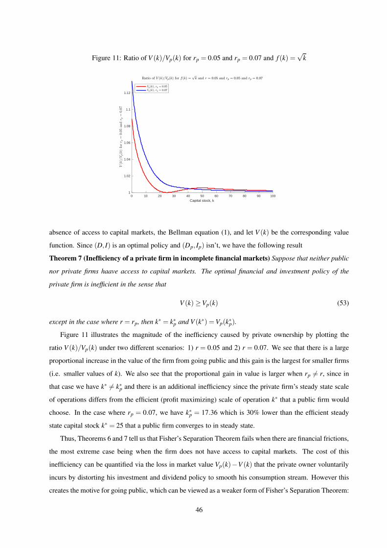
Figure 11: Ratio of V (k)/Vp(k) for rp = 0.05 and rp = 0.07 and f (k) =√

k

0 10 20 30 40 50 60 70 80 90 100

Capital stock, k

1

1.02

1.04

1.06

1.08

1.1

1.12

absence of access to capital markets, the Bellman equation (1), and let V (k) be the corresponding value

function. Since (D, I) is an optimal policy and (Dp, Ip) isn’t, we have the following result

Theorem 7 (Inefficiency of a private firm in incomplete financial markets) Suppose that neither public

nor private firms haave access to capital markets. The optimal financial and investment policy of the

private firm is inefficient in the sense that

V (k)≥Vp(k) (53)

except in the case where r = rp, then k∗ = k∗p and V (k∗) =Vp(k∗p).

Figure 11 illustrates the magnitude of the inefficiency caused by private ownership by plotting the

ratio V (k)/Vp(k) under two different scenarios: 1) r = 0.05 and 2) r = 0.07. We see that there is a large

proportional increase in the value of the firm from going public and this gain is the largest for smaller firms

(i.e. smaller values of k). We also see that the proportional gain in value is larger when rp 6= r, since in

that case we have k∗ 6= k∗p and there is an additional inefficiency since the private firm’s steady state scale

of operations differs from the efficient (profit maximizing) scale of operation k∗ that a public firm would

choose. In the case where rp = 0.07, we have k∗p = 17.36 which is 30% lower than the efficient steady

state capital stock k∗ = 25 that a public firm converges to in steady state.

Thus, Theorems 6 and 7 tell us that Fisher’s Separation Theorem fails when there are financial frictions,

the most extreme case being when the firm does not have access to capital markets. The cost of this

inefficiency can be quantified via the loss in market value Vp(k)−V (k) that the private owner voluntarily

incurs by distorting his investment and dividend policy to smooth his consumption stream. However this

creates the motive for going public, which can be viewed as a weaker form of Fisher’s Separation Theorem:

46

by going public a private owner achieves a separation of ownership and control of the firm, which enables

it to avoid the inefficiency of private ownership and enables the owner to capture the gain in value and

smooth consumption more efficiently in financial markets.

If it is costless to go public and owners do not receive non-pecuniary value/utility from controlling and

running their own private firm, then it is clear from figure 11 that all firms should go public and operate

as risk-neutral expected discounted dividend maximizers. However when there are costs to going public,

things are more complicated. Assume that the fixed costs of an IPO must be paid up front, prior to the IPO.

Define k by f (k) = F . We will also show that when ρ or F are non-zero, there will be another threshold

k > k such that for k > k it is too expensive to go public, and the owner will choose to remain a private

firm.

Theorem 8 (Conditions for going public) Consider a firm that is initially privately held by an owner

whose personal subjective discount rate rp may differ from the market interest rate r at which dividends of

publicly traded firms are discounted at. If the owner can save at interest rate r or if there is an actuarially

fair annuity market which also earns the market return r, then if there are no costs to an IPO, the owner

will always prefer to go public and use the proceeds to save and consume or purchase an annuity, except

if k = 0 or if r = rp and k = k∗, where the owner is indifferent about cashing out or not. If there is a

proportional fee ρ ∈ (0,1) in an IPO, (so the owner only receives the share (1−ρ) of the IPO proceeds),

then only private firms with sufficiently low levels of initial capital k will find it optimal to do an IPO. If

there are also up-front fixed costs F required to do an IPO, then if ρ and F are not too high, there will

be an interval of values of the private owner’s capital stock, [k,k] where it is optimal for the firm to go

public via an IPO. An owner with capital less than k will not have sufficient size to afford the fixed costs

of undertaking an IPO, and an owner with capital greater than k can afford to do the IPO but finds the

transactions costs too high to make it worthwhile.

In the case of no transactions costs to doing an IPO, the proof of Theorem 8 is intuitively clear: we

showed that the private owner has a motive to consumption smooth, but this motive distorts the owner’s

investment policy, since his desire to pay dividends in every period slows the rate of accumulation of capital

to the optimal steady state value k∗. By going public, the newly public firm will avoid these inefficiencies

and the owner can continue to consumption-smooth by using the IPO proceeds to purchase an annuity.

This result is, in effect, a type of separation theorem between investment and consumption. It shows that

in the absence of transactions costs, firms ought to be publicly held rather than privately held, since it is

more efficient to use capital markets than investment policy to smooth out consumption streams. However

if k = 0, then since neither the public or private firm can borrow the owner gets zero in either case and

cannot gain from doing an IPO. If k = k∗, then the firm is already at the optimal steady state capital stock,

and since this results in a flat consumption stream of f (k∗)−δk∗ per period (the same as what an annuity

47

would pay the owner if he sold out), there is no gain from doing an IPO in this case either.

Recall that W (k) represented the welfare (discounted utility) of a private owner who did not have the

option to go public, and did not have access to credit markets. Let Wipo(k) be discounted utility of a private

owner who exercises the option to go public, under the assumption that the owner does a 100% sell out of

his ownership interest. We have

Wipo(k) =u((1−β)[V (k)(1−ρ)−F])

(1−βp). (54)

Wipo(k) represents the value of “stopping” for a private owner, i.e. the value of the option to go public. It

is the discounted utility of the value of an annuity that pays an amount a = (1− β)[V (k)(1− ρ)−F] in

perpetuity that the owner can receive after selling his firm and receiving its market valuation V (k) net of

the proportional and fixed underwriting fees. Let W (k) be the discounted utility for the owner of a private

firm who has the option of going public in the future. Then we have

W (k) =

max0≤I≤ f (k) [u( f (k)− I)+βpW (k(1−δ)+ I)] k < k

max[

Wipo(k),max0≤I≤ f (k) [u( f (k)− I)+βpW (k(1−δ)+ I)]]

k ≥ k

(55)

This equation is similar to the Bellman equation (46) for the owner of a private firm without the IPO

option that we presented in section 4, except that now problem (55) takes the form of an optimal stopping

problem. The solution is defined by a partition of the state space into a continuation region where it is

optimal for the firm to continue to stay private and a stopping region where it is optimal for the firm to

go public. For k < k the firm does not generate enough cash flow to afford the up-front fixed costs to

undertake an IPO, so the owner’s only option is to stay private in this interval with a value given by the

top line of equation (55). However for k ≥ k the owner can afford to undertake an IPO, but his decision

is based on whether net of the proportional costs of the IPO (i.e. net of the fraction ρ deducted from the

sales proceeds V (k) in equation (54)) he will be better off selling out or staying private.

Then the private owner cannot afford to go public if his initial capital stock is in the interval [0,k), so

this is part of the continuation region. We can also show that if ρ is not too large, there will be a unique

value k that satisfies Wipo(k) = W (k) and Wipo(k) < W (k) for k < k and Wipo(k) > W (k) for k > k. Thus

the stopping region is the interval [k,k] and the continuation region consists of the two intervals [0,k) and

(k,∞).

The left hand panel of figure 12 illustrates the gains to going public for a private owner with utility

function u(c) = c.7 where rm = rp = 0.05 and the proportional transactions costs for doing an IPO is ρ = 0.

We see that consistent with Theorem 8, the gains from an IPO are positive for all values of k except k = 0

and k = k∗ = 25 where they are zero. The right hand panel of figure 12 illustrates the gains to going public

when ρ = 0.07 and the fixed fee F = 0.5. The 7 percent commission rate is typical for IPOs underwritten

48

Figure 12: Effect of transactions costs ρ on the value of going public

Capital Stock0 5 10 15 20 25 30 35 40 45 50

Dis

coun

ted

Util

ity G

ain

from

Sel

ling

Out

0

0.5

1

1.5

2

2.5

3

3.5Utility Gains to Private Owner from an IPO, ρ=0

Capital Stock0 1 2 3 4 5 6 7 8 9 10

Dis

coun

ted

Util

ity G

ain

from

Sel

ling

Out

-1.5

-1

-0.5

0

0.5

1

kl

ku

Utility Gains to Private Owner from an IPO, ρ=0.07

by investment banks in the US and other countries. We see with the higher commission rate, the gains

from doing an IPO are negative for k > k = 2.75, and also an owner who has no access to credit markets is

unable to afford the fixed cost of the IPO when k < k = .25 since the cash flow f (k) =√

k is insufficient to

enable the owner to pay F in this case. So the interval [k,k] = (.25,2.75) represents the optimal stopping

region in this case: the interval of capital where it is optimal for the owner to take his firm public with an

IPO and then sell out.

We see that in the presence of transactions costs, it is no longer better to go public regardless of

the initial capital stock of the firm. It is only optimal for firms that are in the “goldilocks zone” with a

minimal amount of capital to be able to afford the fixed costs of an IPO but not too much capital where the

commission constitutes an unacceptably large tax on the owner. In addition, as the private firm’s capital

gets close to k∗, the incentive to do an IPO falls as we showed in Theorem 8, since the firm is close to

a point where it can reach k∗ quickly anyway using its own retained earnings. Thus, we have succeeded

already in providing an answer to both “why” and “when” private firms go public.

Now we consider an additional motivation for a firm to go public: access to credit markets. It is

often claimed that due to agency reasons and information costs, public firms have superior access to credit

markets than private firms. We will start by considering the most extreme case where the owner has no

ability to borrow as a private firm but if the firm were public, it would face no borrowing constraints.

Clearly, when this is the case the incentive to go public is enhanced, since we have already shown how the

ability to borrow increases the value of a public company.

Corollary 8.1 (Access to credit markets enhances the value of going public) Suppose the assumptions

of Theorem 8 hold except that public firms have unlimited access to credit markets and face no borrowing

constraints at an interest rate rb = rm. Then the incentives for going public are higher, and when there are

both fixed and proportional transactions costs to undertaking an IPO, the interval of capital [k,k] where

49

Figure 13: Gains to going public with ρ = 0.07 when post-IPO public firm has access to credit markets

Capital Stock0 1 2 3 4 5 6 7 8 9 10

Dis

coun

ted

Util

ity G

ain

from

Sel

ling

Out

0

5

10

15

20

25

30

35

kl

ku

Utility Gains from Selling Out for Private Owner with No Debt

it is optimal for the owner to do an IPO is larger than in the case where public firms have no access to

capital markets.

Figure 13 illustrates Corollary 8.1 by plotting the gains to going public, Wipo(k)−W(k), in the case

where the post-IPO public firm has full access to credit markets and can borrow unlimited amounts at

rb = 0.05, the same as the owner’s personal interest rate and the rate at which the public firm’s dividends

are discounted. The biggest gain to going public now occurs at k = 0: an owner with no initial capital

cannot borrow as a private firm and thus cannot get his firm off the ground. But once the firm goes public

it obtains access to credit markets, which enables the firm to borrow enough to attain the optimal steady

state capital stock k∗ with only a single period delay. Thus, the owner of a private firm is able to unlock

tremendous value by the act of going public, and in effect, gain access to credit in an indirect manner that

would not be possible for him to do if the firm remained private.

We can see from figure 13 that due to the increased value that access to credit markets confers on the

post-IPO public firm, the interval of capital [k,k] for which going public is optimal widens from [.25,2.75]

to [.25,5]. We can see that the gains to doing an IPO decline very rapidly as k increases, and private firms

with the least capital are the ones that gain the most from going public. Underwriters of IPOs might take

note of this and waive any up-front fixed fees for doing an IPO for the smallest private firms in exchange

for a larger commission ρ. For example if the underwriter waived the fixed fee, F = 0 and raised the

commission from ρ = 0.07 to ρ = 0.08, it would capture new business from the smallest private firms and

the incremental commission revenue (since the valuation of a new public firm is V (0) = 50), makes up

for lost fixed fee. However fewer medium-sized private firms would do IPOs, since k falls from 5 when

ρ = .07 to k = 4.25 when ρ = 0.08.

Finally, suppose both private and public firms have equal (unlimited) access to credit markets at an

50

interest rate rb = rm = rp. Then the gain to doing an IPO drops precipitously, and unless the transactions

costs of doing an IPO are zero, no private firms will choose to go public. This follows because with

unlimited ability to borrow, as we will showed in Fisher’s Separation Theorem (Theorem 4 of section 4),

the private owner is able to reach the efficient steady state k∗ in the first period, after which the private

owner achieves the same dividend stream in perpetuity as a public firm produces.

Corollary 8.2 (Access to credit markets by a private held firm reduces the value of going public) If

the owner of the privately held firm has access to credit markets, the incentives for undertaking an IPO

are dramatically reduced, and unless the transactions costs associated with undertaking an IPO are near

zero, the private owner will have no incentive to go public. The incentives for going public are stronger

if: a) the borrowing constraints the private owner faces are tighter, and b) the owner of the private firm is

encumbered with initial debt.

Results a) and b) of Corollary 8.2 are intuitively clear, but order to formally prove that they hold we

need to extend the private owner’s investment and financing problem to account for debt financing and

credit constraints, and the possibility that in order to start the firm the founder may have to go into debt

to finance the acquistion of the production technology f and initial capital stock k, but due to borrowing

constraints, the owner cannot borrow enough to reach the efficient steady state capital stock k∗ imediately.

We will consider this extension of the private owner’s problem in section 6 and show how too much initial

debt can encumber the private firm and increase the incentives for doing an IPO.

5.1 Using IPOs to raise new capital

As we noted in section 2 most IPOs do not entail a 100% sell-off of the original owner’s stake in the

company. Instead, the original owner retains a partial ownership stake in the firm, and only takes part of

the IPO proceeds in cash to finance consumption or other investment projects. The other important role

of a partial cash-out is that when the original owner continues to own a significant share of the post-IPO

company, the share of the IPO proceeds that the owner does not cash out can be re-invested in the company,

thereby providing a new infusion of capital to the firm after the IPO that is not reflected in our analysis of

an IPO with a 100% cash out by the original owner.

The cash raised in an IPO thus has similarities to the proceeds of a loan: in each case the original

owners have “sold off” some of the future dividends of the company in order to finance current investment.

When the returns from investment are sufficiently high, the increased value from the investment in the firm

outweighs the future claims of debt-holders or new shareholders, increasing the overall equity value of the

original owner compared to a scenario of a 100% sell off that we considered in section 5. In this section

we characterize the conditions under which the original owner will want to do an IPO but retain only a

partial ownership stake in the post-IPO company and reinvest some or all of the capital raised in the IPO.

51

Thus, an IPO benefits the owner in two different ways: 1) the IPO changes the objective function of

the firm from utility maximization to discounted value maximization, benefitting the original owner by

eliminating what we might call the dividend smoothing inefficiency of private ownership, and 2) the IPO

provides an infusion of new capital that the original owner can use to reinvest back into the company.

Suppose the firm is originally a privately owned firm by a sole owner, and the owner chooses to take

the firm public via an IPO and retain only a fraction α ∈ (0,1) of his/her original 100% ownership stake

in the firm. Thus, after the IPO the original owner will own a fraction α of the firm (i.e. α is fraction of

shareholdings still owned by the founder of the firm) and the outside investors who bought shares in the

new firm will own the remaining fraction 1−α of the firm’s shares.

The IPO proceeds equal the total amount the founder receives from selling shares in the newly public

firm to the new outside investors, net of the underwriting fees. Mathematically, at least in terms of our

formulation of a fixed point condition that determines the proceeds raised, an IPO is equivalent to the case

of a SEO that we introduced in equation (28) of section 3.3. In particular, the founder can either reinvest

the net proceeds to increase the capital stock (and hence future profit/dividend stream of the firm), or cash

out some or all of the proceeds for private consumption or investment purposes (e.g. to buy an annuity

or invest in another venture). As in the case of an SEO we let ω ∈ [0,1] represent the fraction of the IPO

proceeds that the owner chooses to take out for consumption or other investment purposes, and thus the

fraction 1−ω of the net IPO proceeds is reinvested in the firm.

There is, of course, a key practical difference between a SEO and an IPO. In a SEO there is much

more of a “track record” and more information available to potential new shareholders about the company

and its prospects. In an IPO, there is less information about the new company given that it has been run

as private operation until the point where the IPO takes place. Information about the prospective new

company is provided in a prospectus prepared by an underwriter as one of their key services in conducting

the IPO.8 Part of the concern and risk to new shareholders considering investing in an IPO is the possibility

that the founder might “take the money and run” after the IPO. One of the key functions provided by an

underwriter is to do the due diligence to investigate the private firm that wishes to go public with an IPO

and certify to investors that the company really does exist and the founder will not “take the money and

run” after an IPO. Thus, the reputation of the underwriter, in addition to market regulation (such as is

done by government agencies such as the Securities and Exchange Commission), helps convince outside

investors that an IPO is legitimate and is not a thinly disguised take the money and run scheme.

However we believe that as a first approximation that information on the firm’s production technology

f , its initial capital k, and the founder’s choice of (α,ω) can be treated as credible common knowledge to

8As Draho [2004] notes, “The prospectus is usually the first source of information about the issuer available to investors, astheir is rarely anything published prior to the IPO (Rao 1993). The prospectus provides a thorough overview of the firm, itsoperations and structure, intended use of proceeds and terms of the offering.” (p. 164).

52

Figure 14: Value of founder’s post-IPO wealth for different (α,ω) values

011

10

0.80.8

20

Cas

h fr

om IP

O p

lus

valu

e of

foun

der's

sha

res

0.60.6

30

40

0.40.4

50

0.20.2

00

investors that is revealed by the due diligence of the underwriter and communicated in the prospectus for

the IPO. Of course the underwriter incurs costs of doing the due diligence and preparing the prospectus,

and advertising the new issue to attract a sufficient number of new investors, and providing liquidity and

avoid adverse price impacts by selling too many shares too quickly. that a private firm that wants to go

public via an IPO is legitimate. Some underwriters provide insurance to the founder via a firm-commitment

contract that fully or partially guarantees some level of proceeds from the IPO as discussed in section 2.2.

The underwriter is compensated for this risk and its services by charging a proportional fee ρ ∈ (0,1) plus

a fixed fee F . Thus if the gross proceeds of the IPO are P(k,α,ω), the net proceeds received by the founder

from the investment bank (after it deducts its fees) are (1−ρ)P(k,α,ω)−F .

Figure 14 plots the value of the founder’s post-IPO wealth (the sum of the amount cashed out from the

IPO plus the value of the shareholding in the post-IPO company that the founder retains) as a function of

(α,ω) for k = .25, the smallest level of k that enables the firm to afford the fixed costs of the IPO: f (.25) =

.5. In equation (36) of section 3.3 we defined the function W (k,α,ω) to represent the total wealth of

the original shareholders after an SEO, and this same function also characterizes the founder’s total wealth

after an IPO. Although it is difficult to see from figure 14, when ρ> 0 and F > 0, the function W (k,α,ω) is

no longer symmetric in its (α,ω) arguments. For example, W (.25, .7, .2) = 48.68 6=W (.25, .2, .7) = 46.43.

Figure 15 provides further on the impact of the α and ω parameters detail by plotting slices of the

function W (k,α,ω). The left hand panel of figure 15 shows how the value of the firm varies with α when

we fix ω = .2. Of course, the IPO proceeds must equal 0 when α = 1 and the value of the post-IPO firm

increases monotonically as α decreases. This is due to the fact that the founder is reinvesting ω = .2 of the

53

Figure 15: Value of founder’s post-IPO wealth as a function of α and ω

0 0.1 0.2 0.3 0.4 0.5 0.6 0.7 0.8 0.9 1

Fraction post IPO firm owned by founder‘,

0

20

40

60

80

100

120

140

160

180

Val

ue o

f firm

, am

ount

inve

sted

Value of firm, post IPOIPO ProceedsIPO Proceeds reinvestedValue of founder's cash+equity

0 0.1 0.2 0.3 0.4 0.5 0.6 0.7 0.8 0.9 1

Fraction IPO proceeds cashed out,

0

10

20

30

40

50

60

70

80

90

Val

ue o

f firm

, am

ount

inve

sted

Value of firm, post IPOIPO proceedsIPO proceeds reinvestedValue of founder's cash+equityValue of Founder's shares

IPO proceeds back in the firm and thus the larger the fraction of firm the founder sells off (i.e. the smaller

is α), the greater the amount that is reinvested, thereby increasing the value of the firm. The solid black

line plots the net IPO proceeds and the dashed line plots the share of the net proceeds that are reinvested

(the remaining proceeds are used to pay dividends). In this case, the value of the founder’s total wealth

(cash taken out plus ownership in the post-IPO firm) is maximized when α = .739, resulting in total wealth

of W (.25, .739, .2) = 48.73.

The right hand panel of figure 15 shows how the founder’s wealth varies with ω when α is fixed at

α = .5. Of course, the total post-IPO equity value (red line in the figure) is maximized when ω = 0

since the founder has reinvested all of the net IPO proceeds back into the company. However this does not

maximize the founder’s wealth since the outside investors are receiving half of the benefits of the founder’s

investment of the IPO proceeds. The founder’s total wealth is maximized by setting ω= .4686, resulting in

total wealth of W (.25, .5, .4686) = 47.80. By cashing out this relatively large share of the net IPO proceeds

the founder leaves the company with insufficient funds to reach the optimal steady state capital stock k∗.

In comparison, when ω = 0, the net proceeds are W (.25, .5,0) = 43.16, which exceeds the capital the firm

needs to invest to reach k∗ = 25. So the firm pays out difference, 43.16− 25 = 18.16, as cash dividends

and the founder receives half of this amount.

When we simultaneously optimize over (α,ω) which combination maximizes W (k,α,ω)? Intuitively,

it should not be optimal for the founder to use any of the net IPO proceeds for cashing out if the return

from investing these proceeds has a sufficiently high rate of return. Of course, there is a “tax” of ρ imposed

by the underwriter on each dollar raised in the IPO. Cashing out these “after tax” dollars has a marginal

return of 1 (i.e. alllocating one dollar of the net IPO proceeds to cashing out increases the founder’s

wealth by one dollar). However reinvesting the marginal dollar back into the firm has a marginal return

of αβV ′(k+P(k,α,ω)(1− ρ)−F). As long as this latter rate of return is greater than 1, the founder is

54

better off reinvesting the marginal dollar from the net IPO proceeds rather than cashing out. This will be

the case if after receiving the net IPO proceeds, the firm is still in the “investment region” in equation (27)

where it optimally allocates all resources to investment and pays no dividends. This will be the case when

the initial capital stock k is sufficiently low andα is sufficiently high, i.e. when the founder has retained a

sufficiently large ownership share of the post-IPO firm. We summarize this login in Theorem 9 below.

Theorem 9 If ρ > 0 then W (k,α,ω) is not symmetric in (ω,α). For sufficiently large α W (k,α,ω) is

decreasing in ω. Thus, the value of (α∗,ω∗) that maximizes W (k,α,ω) satisfies ω∗ = 0, i.e. if a wealth-

maximizing founder chooses to take his company public, he will choose to reinvest all of the net IPO

proceeds back into the company.

To illustrate Theorem 9, consider a founder who has initial capital, k = 0.25 which is just sufficient to

pay for the fixed cost of an IPO, F = 0.5. If the owner were to sell 100% of his firm and not reinvest any

of the proceeds (i.e. α = 1 and ω = 1) the owner’s wealth would be W (.25,1,1) = 42.68, which equals

βV (k(1−δ)) since the fixed cost of the IPO consumes the firm’s entire cash flow, so it can neither invest

nor pay dividends in the period it goes public. The the optimal IPO occurs at the parameters (α∗,ω∗) =

(.776,0) which yields the owner a post-IPO total wealth of W (.25, .776,0) = 48.96. The founder is better

off from doing the IPO, since even net of the fixed fee for doing the IPO, F = 0.5, his wealth is higher

from selling off (1−α∗) = 0.224 of the firm, and using the net IPO proceeds to reinvest in the company.

Note that the gross IPO proceeds equal P(.25, .776,0) = 14.15, and net proceeds are P(.25,776,0)(1−ρ)−F = 12.66. When these proceeds are added to the initial capital k = 12.91 < k∗ = 25, so it follows

that βV ′(k+P(k,α∗,0)(1−ρ)−F) > 1, confirming the conclusion of Theorem 9 that it is better for the

founder to reinvest all of the net proceeds from the IPO back into the firm rather than take any of this out in

cash. Further, since the post-IPO public firm is still in the “liquidity constrained region” (the region where

k < k where k is the threshold defined in equation (7) of section 2), no dividends will be paid after the IPO.

Note that after the IPO, if the newly formed public company does not have access to debt markets and

thus cannot borrow, it may want to raise the additional capital to reach the optimal steady state capital

stock k∗ as quickly as possible by doing an SEO. However referring to figure 7, even under the best case

“Modigliani-Miller” scenario where the firm either has access to unlimited credit can do an SEO at zero

cost, the gains to using additional external sources of finance are quite small once k = 12.91, compared

to financing the remaining capital needs by retained earnings. Thus if SEO costs involve a commission

of ρ = 0.07 and F = 0.5, in this particular example it would not be optimal for the post-IPO firm to turn

around and do a follow-on SEO as well.

We are now in position to characterize the conditions under which it is optimal for the owner of a

private firm to go public with an optimally structured IPO. At the risk of some notational confusion, we

define the function Wipo(k) which unlike the function with the same name defined in equation 54 above,

55

Figure 16: Gains to going public, Wipo(k)−W(k), and α∗(k) when (ρ,F) = (.07, .5)

0 5 10 15 20 25 30

Capital stock, k

20

22

24

26

28

30

32

Dis

coun

ted

utili

ties

W(k), value of staying privateW ipo(k), value of going public

0 5 10 15

Capital stock, k

0.75

0.8

0.85

0.9

0.95

1

but now instead of the total wealth of the founder, we let Wipo(k) represent the discounted utility of the

founder after an “optimal” IPO and after this resulting wealth is converted into an annuity, i.e.

Wipo(k) =u((1−β)[maxα,ωW (k,α,ω)])

(1−βp). (56)

In fact, we can show that the owner is also better off from conducting an optimal IPO rather than continuing

to run his company as a private firm: Wipo(k)>W (k) when k = 0.25.

The left hand panel of figure 16 plots the two value functions W (k) (the value function for the private

firm owner without the option of going public, equation (46) in section 5) and Wipo(k) defined in equa-

tion (56) above. Due to our assumption that the fixed costs of the IPO must be paid up front, the IPO is not

feasible until the capital stock exceeds k = .25 since f (k) = F . Let k be the smallest value of k for which

Wipo(k) =W (k). Then we see from figure 16 that for k ∈ (k,k) = (.25,17.31) we have Wipo(k)>W (k) and

this constitutes the “goldilocks region” where it is optimal for the owenr to go public. For k > k and suf-

ficiently close to the optimal steady state capital stock k∗ = 25, we have W (k)>Wipo(k), i.e. it is optimal

for the owner to remain private in this region, since the costs of doing an IPO outweigh the benefits.

The right hand panel of figure 16 plots the optimal dilution value α∗(k). We see it increases monotoni-

cally from α∗(.25) = .77 at the lower threshold k = .25 for the “stopping region” where it is optimal to go

public, and reaches α∗(k) = 1 at k = 11.22. Thus, the financing value of doing an IPO quickly disappears

as k increases and the owner’s motive for going public switches to the desire for liquidity and eliminating

what we previously terms the dividend smoothing inefficiency of private ownership. There is a higher

threshold of capital, k̂ > k∗ not shown in figure 16 beyond which it is optimal for the firm to go public

again, i.e. Wipo(k)>W (k) for k > k̂ = 35.11. Why would this be the case?

The reason is that when k > k̂ > k∗ the private owner is “overcapitalized” since his capital stock is

above the optimal steady state value of k∗ = 25. Referring back to figure 9, we see that due to the dividend

56

smoothing inefficiency the private owner still invests at k = k̂ but at a value that not enough to offset

depreciation, so the capital stock will gradually shrink back to k∗. This implies that dividends will be

slowly declining while the capital shrinks, leading the private owner to experience a temporary period of

declining dividends and thus consumption. Because of our putty-clay assumption on the capital stock, the

private owner cannot simply liquidate a portion of the capital stock to smooth out his consumption stream.

Instead, it is optimal for the owner to take his company public so that it can be managed more efficiently

and enable the owner to capture part of this efficiency gain (net of the cost of the IPO) and more efficiently

smooth his consumption stream using financial markets (e.g. annuities). Refer back to figure 11 which

illustrates the relatively small efficiency gains to be had from going public even by overcapitalized private

firms.

To fully and rigorously define the optimal decision making of a private owner when he has the option

of going public, we solve the Bellman equation given in equation (55) of section 5 for the 100% sell out

case (α = 1) but with Wipo(k) replaced by the value under an optimally done IPO givem in equation (56)

above. We summarize this discussion in

Theorem 10 (the IPO decision as an optimal stopping problem) Assume neither the public or private

firms have access to debt markets, but can raise external equity via a costly IPO with commission rate ρ> 0

and fixed costs F > 0. Let γ(k) be the private owner’s optimal stopping rule, where γ(k) = 1 denoting a

decision to go public with an optimally chosen IPO and γ(k) = 0 denoting the decision to remain private.

We have

γ(k) =

0 if k ≤ k

1 if k ∈ (k,k)

0 if k ∈ [k, k̂)

1 if k > k̂

(57)

where k < k < k∗ < k̂.

We regard the possibility private firm might be overcapitalized (i.e. the case k > k̂ in Theorem 10) to

be a theoretical curiosum, since normal investment dynamics should never lead a private firm to become

overcapitalized in the first place. It could possibly be relevant if an exogenous technological improvement

enabled the firm to adopt a new more technologically efficient production function f1(k) in place of their

existing production technology f (k) and the new production technology has an optimal steady state capital

stock k∗1 that is less than the steady state capital k∗ for production function f (k). In such situations it may be

that overcapitalization is empirically relevant and cold be a motive for even a large private firm to go public,

especially if there are large investment costs involved to convert the firm from production technology f to

the new technology f1.

57

Figure 17: Gains to going public, Wipo(k)−W (k), and α∗(k) when (ρ,F) = (.2,2)

0 5 10 15 20 25 30

Capital stock, k

20

22

24

26

28

30

32

Dis

coun

ted

utili

ties

W(k), value of staying privateW ipo(k), value of going public

0 5 10 15

Capital stock, k

0.75

0.8

0.85

0.9

0.95

1

As we noted from the work of Ritter [1987] in section 2.2 the cost of an IPO is much higher when the

effect of underpricing of new issues is taken into account. Figure 17 shows the gains to going public when

we set (ρ,F) = (.2,2), where the ρ = .2 value was motivated by low end of the estimates of Ritter [1987]

on the cost of an IPO. We see that the increase in IPO costs dramatically shrinks the range of capital stocks

over which it is optimal for the private owner to go public, from [k,k] = [.25,17.36] when ρ = .07 and

F = .5 to [k,k] = [2,9.94], or decreasing the width of this interval by more than 50%. We also see from the

right hand panel of figure 17 that the share of the firm that the owner is willing to sell to outside investors

is significantly reduced as well, from 15% when k = 4 and (ρ,F) = (.07, .5) to 8% when (ρ,F) = (.2,2).

5.2 IPOs in the non-concave case

This section briefly describes a complication that can occur in the case of non-concave production func-

tions f (k), such as the example we studied in section 3.1. A key issue is the potential for multiple fixed

points to the condition defining SEO and IPO proceeds in equation (28) of section 3.3. Figure 18 illustrates

the problem, for a case where there are a total of 4 IPO fixed points.

We argue that the solution to this problem is to pick the largest fixed point. In this case the largest fixed

point results in gross IPO proceeds of P(k,α,ω) = 234.03 when k = 0, α = .35 and ω = 0. The reason

why we choose this fixed point is 1) the owner strictly prefer larger IPO proceeds, and 2) we assume that

via the IPO prospectus that the owner can credibly signal to outside investors the level of reinvestment

he plans for the IPO proceeds, and this in effect acts as an “equilibrium selection mechansim”. Thus, we

argue that the private owner has the ability to select the IPO “equilibrium” which is best for him in cases

where there may be multiple IPO fixed points to equation (28). After this small adjustment, our analysis

of IPOs for firms with non-concave production functions proceeds in the same way as we did for a firm

58

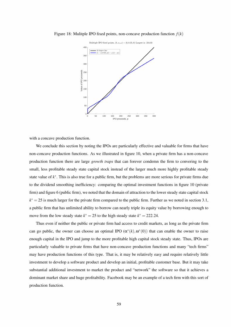
Figure 18: Mulitple IPO fixed points, non-concave production function f (k)

0 50 100 150 200 250 300 350 400

IPO proceeds, p

0

50

100

150

200

250

300

350

400

Val

ue o

f IP

O p

roce

eds

with a concave production function.

We conclude this section by noting the IPOs are particularly effective and valuable for firms that have

non-concave production functions. As we illustrated in figure 10, when a private firm has a non-concave

production function there are large growth traps that can forever condemn the firm to convering to the

small, less profitable steady state capital stock instead of the larger much more highly profitable steady

state value of k∗. This is also true for a public firm, but the problems are more serious for private firms due

to the dividend smoothing inefficiency: comparing the optimal investment functions in figure 10 (private

firm) and figure 6 (public firm), we noted that the domain of attraction to the lower steady state capital stock

k∗ = 25 is much larger for the private firm compared to the public firm. Further as we noted in section 3.1,

a public firm that has unlimited ability to borrow can nearly triple its equity value by borrowing enough to

move from the low steady state k∗ = 25 to the high steady state k∗ = 222.24.

Thus even if neither the public or private firm had access to credit markets, as long as the private firm

can go public, the owner can choose an optimal IPO (α∗(k),ω∗(0)) that can enable the owner to raise

enough capital in the IPO and jump to the more profitable high capital stock steady state. Thus, IPOs are

particularly valuable to private firms that have non-concave production functions and many “tech firms”

may have production functions of this type. That is, it may be relatively easy and require relatively little

investment to develop a software product and develop an initial, profitable customer base. But it may take

substantial additional investment to market the product and “network” the software so that it achieves a

dominant market share and huge profitability. Facebook may be an example of a tech firm with this sort of

production function.

59

6 Extensions and Caveats

Not yet completed.

7 Conclusions

This paper introduced a simple theory of why and when firms go public. These are our main results:

Why go public? Because risk aversion and the desire of a private owner to consumption smooth

causes him/her to distort their investment and financial policy, resulting in slower growth and less

ambitious operation of the company. Though the behavior of the owner is privately optimal it is

sub-optimal with respect to the criterion of maximization of market value of the firm. Provided the

fixed and variable transaction costs of undertaking an IPO are not too high, the owner can gain by

taking the firm public so it can be run by a risk-neutral manager in a way that maximizes the present

value of dividends, and thus the equity valuation of the company.

When to go public? We showed that especially for firms with a non-concave production function

(which we argued is relevant for firms that undergo multiple stages of growth as they evolve from

a small scale firm with little capital to a large scale firm with a large capital stock that can exploit

significant global returns to scale from expansion), the optimal time to go public is when the firm

is at the “Goldilocks size” — not too small and not too big. Firms that are too small and which

face borrowing constraints that prevent them from investing to quickly reach the efficient scale of

operations will not experience large returns from going public, and will not be able to afford the

significant fixed and proportional transactions costs of an IPO. Firms that have already acquired a

large capital stock can afford to do an IPO but have already have nearly the level of capital they need

to to achieve the efficient scale of operation, and so can easily use a combination of debt financing

and retained earnings to acquire the remaining capital necessary to achieve their optimal scale.

Our theory is only a beginning. There are many ways to extend our simple model to make it more

realistic such as adding uncertainty and learning as we discussed in section 6. Our eventual goal is to use

this theory as a basis for structural estimation of the IPO decision using panel data on Indian firms over

the period 1990 to 2005. Such an exercise can help us determine whether our theory really is capable of

providing a good approximation to the behavior of actual firms, and explaining why some firms go public

and others don’t.

Our theory can be extended to incorporate the impact of various types of regulations and policies

affecting IPOs, including regulations such as the Sarbanes-Oxley Act that was passed in the wake of

60

the Enron debacle and was designed to improve accounting, financial disclosures, company oversight

and corporate responsibility. It remains an open question whether well intended regulations designed to

prevent corporate abuses have had unintended effects that have contributed to the decline in IPOs. As Ritter

argues, “It is possible that, by making it easier to raise money privately, creating some liquidity without

being public, restricting the information that stockholders have access to, restricting the ability of public

market shareholders to constrain managers after investors contribute capital, and driving out independent

research, the net effect of the JOBS Act might be to reduce the flow of capital into young high-technology

companies or the number of IPOs of small emerging growth companies.”

However our theory suggests it is not just regulatory burdens that could contribute to the trend: we

find that the costs of undertaking IPOs, with the large 7% underwriting commission and associated fixed

costs, can also be a significant deterrent of using IPOs to finance growth relative to debt financing or

retained earnings. But most importantly it is the owner’s expectations and beliefs about the potential gains

to significant capital investments that is a decisive driver of the decision to do an IPO. If competition in the

product market is tougher making it harder for newly ascending companies to break the “glass ceiling” of

competition from larger well established rivals, then even drastic reductions or even outright elimination

of regulatory burdens and reductions in the investment banking costs of doing IPOs (perhaps via policies

that encourage freer entry into the underwriting sector) may not have a significant effect on the number

of IPOs, especially with the expansion of “private capital” and “venture capital” as alternative potentially

more efficient alternative to IPOs. As Decker et. al. note, “Theo open question is why firms with high

realizations of productivity, especially those in the High Tech sector, do not experience the same high

growth as before.”

References

Aydogan Alti. Ipo market timinig. Review of Financial Studies, 18(3):1105–1138, 2005.

J. Ang and J. Brau. Concealing and confounding adverse signals: Insider wealth-maximizing behavior inthe ipo process. Journal of Financial Economics, 67:149–172, 2003.

Simon Benninga, Mark Helmantel, and Oded Sarig. The timing of initial public offerings. Journal ofFinancial Economics, 75:115–132, 2005.

Mikael C. Bergbrant, Daniel Bradley, and Delroy M. Hunter. Does bank loan supply affect the supply ofequity capital? evidence from new share issuance and withdrawal. Journal of Financial Intermediation,29:32–45, 2017.

Andriy Bodnaruk, Eugene Kandel, Massimo Massa, and Andrei Simonov. Shareholder diversification andthe decision to go public. The Review of Financial Studies, 21(6):2779–2824, 2008.

Julie Bort. Why startup founders happily give up 90% of their companies. Business Insider, 2014.

J. Brau, M. Li, and J. Shi. Do secondary shares in the ipo process have a negative effect on aftermarketperformance? Journal of Banking and Finance, 31(9):2612–2613, 2007.

61

J. C. Brau, I. Degraw, and P. Ryan. Initial public offerings: Cfo perceptions. Financial Review, 41:483–511, 2006.

James Brau. Why do firms go gublic? In Douglas Cumming, editor, Oxford Handbook of EntreprenurialFinance, pages 467–494. New York: Oxford University Press, 2012.

A. Brav, J.R. Graham, C. R. Harvey, and R. Michaely. Payout policy in the 21st century. Journal ofFinancial Economics, 77:483–527, 2005.

M. J. Brennan and J. Franks. Underpricing, ownership and control in initial public offerings of equitysecurities in the uk. Journal of Financial Economics, 45(3):391–414, 1997.

Thomas J. Chemmanur and Paolo Fulghieri. A theory of the going-public decision. The Review of Finan-cial Studies, 12(2):249–279, 1999.

Thomas J. Chemmanur and Jie He. Ipo waves, product market competition, and the going public decision:Theory and evidence. Journal of Financial Economics, 101(2):382–412, 2011.

Thomas J. Chemmanur, Shan He, and Debarshi K. Nandy. The going-public decision and the productmarket. The Review of Financial Studies, 23(5):1855–1908, 2009.

H. Chen and J. Ritter. The seven percent solution. Journal of Finance, 55:1105–1131, 2000.

Jiri Chod and Evgeny Lyandres. Strategic ipos and product market competition. Journal of FinancialEconomics, 100(1):45–67, 2011.

Gian Luca Clementi. Ipos and the growth of firms, 2002.

Thomas F. Cooley and Vincenzo Quadrini. Financial markets and firm dynamics. American EconomicReview, 91(5):1286–1310, 2001.

Anupreeta Das. Paying debt with ipo proceeds? investors may not buy. Reuters Market News, 2008.

Ryan A. Decker, John Haltiwanger, Ron S. Jarmin, and Javier Miranda. Declining dynamism, allocativeefficiency, and the productivity slowdown, 2016.

Ryan A. Decker, John Haltiwanger, Ron S. Jarmin, and Javier Miranda. Declining dynamism, allocativeefficiency, and the productivity slowdown, 2017.

Francois Degeorge and Richard Zeckhauser. The reverse ipo decision and firm performance: Theory andevidence. Journal of Finance, 48:1323–1348, 1993.

Jason Draho. The IPO Decision: Why and How Companies Go Public. Edward Elgar, Northampton, MA,2004.

Eugene F. Fama and Kenneth R. French. New lists: Fundamentals and survival rates. Journal of FinancialEconomics, 73:229–269, 2004.

Eugene F. Fama and Michael C. Jensen. Separation of ownership and control. Journal of Law andEconomics, 26(2):301–325, 1983.

Irving Fisher. The Theory of Interest. New York: The MacMillan Co., 1930.

C. Fritz Foley and Robin Greenwood. The evolution of corporate ownership after ipo: The impact ofinvestor protection. Review of Financial Studies, 23(3):1231–1260, 2010.

Drew Fudenberg and Jean Tirole. A theory of income and dividend smoothing based on incumbency rents.Journal of Political Economy, 103(1):75–93, 1995.

Sudip Gupta and John Rust. Going public in india: A structural empirical analysis, 2018.

Ilan Guttman, Ohad Kadan, and Eugene Kandel. Dividend stickiness and strategic pooling. Review ofFinancial Studies, 23(12):4455–4456, 2010.

R. G. Ibbottson and J. F. Jaffe. ‘hot issue’ markets. Journal of Finance, 30:1027–1042, 2005.

Bharat A. Jain and Omesh Kini. The post-issue operating performance of ipo firms. Journal of Finance,49(5):1699–1726, 1994.

62

David Javakhadze, Stephen P. Ferris, and Nilanjan Sen. An international analysis of dividend smoothing.Journal of Corporate Finance, 29:200–220, 2014.

Michael C. Jensen and William H. Meckling. Theory of the firm: Managerial behavior, agency costs andownership structure. Journal of Financial Economics, 3(4):305–360, 1976.

Brian Johnson, David Westenberg, Erika Robinson, and Lia Der Marderosian. 2017 ipo report, 2017.

Martin Kenney, Donald Patton, and Jay R. Ritter. Post-ipo employment and revenue growth for u.s. ipos,june 19962010, 2012.

Woojin Kim and Michael S. Weisbach. Motivations for public equity offers: An international perspective.Journal of Financial Economics, 87:281–307, 2008.

Mark T. Leary and Roni Michaely. Determinants of dividend smoothing: Empirical evidence. Review ofFinancial Studies, 24(10):3197–3249, 2011.

Ilya Levtov. How much equity do founders have when their company ipos? Priceonnmics, 2016.

John Lintner. Distribution of incomes of corporations among dividends, retained earnings, and taxes.American Economic Review, 46:97–113, 1956.

A. Ljungqvist and W.J. Wilhelm. Ipo allocations: Discriminatory or discretionary? Journal of FinancialEconomics, 65:167–201, 2002.

Michelle Lowry and G. William Schwert. Ipo market cycles: Bubbles or sequential learning? Journal ofFinance, 67(3):1171–1198, 2002.

Deborah J. Lucas and Robert L. McDonald. Equity issues and stock price dynamics. Journal of Finance,45(4):1019–1043, 1990.

Jonathan Macey. As ipos decline, the market is becoming more elitist. Los Angeles Times, January(10),2017.

Vojislav Maksimovic and Pegaret Pichler. Technological innovation and initial public offerings. Reviewof Financial Studies, 14(2):459–494, 2001.

Roni Michaely and Michael R. Roberts. Corporate dividend policies: Lessons from private firms. Reviewof Financial Studies, 25(3):711–746, 2011.

Wayne H. Mikkelson, M. Megan Partch, and Kshitij Shah. Ownership and operating performance ofcompanies that go public. Journal of Financial Economics, 44:281–307, 1997.

Franco Modigliani and Merton Miller. The cost of capital, corporation finance and the theory of invest-ment. American Economic Review, 48(3):261–298, 1958.

Adlai Fisher Murray Carlson and Ron Giammarino. Corporate investment and asset price dynamics:Implications for seo event studies and long-run performance. Journal of Finance, 61(3):1009–1034,2006.

Marco Pagano. The flotation of companies on the stock market: a coordination failure model. EuropeanEconomic Review, 37:1101–1125, 1993.

Marco Pagano, Fabio Panetta, and Luigi Zingales. Why do companies go public: An empirical analysis.Journal of Finance, 53(1):27–63, 1998.

Lubos Pastor, Lucian A. Taylor, and Pietro Veronesi. Entrepreneurial learning, the ipo decision, andthe post-ipo drop in firm profitability. The Review of Financial Studies, 22(8):3005–3046, 2009. doi:10.1093/rfs/hhn082. URL + http://dx.doi.org/10.1093/rfs/hhn082.

Edmund Phelps. Golden Rules of Economic Growth. New York: Norton, 1966.

Jay R. Ritter. The costs of going public. Journal of Financial Economics, 19:269–281, 1987.

Jay R. Ritter. Reenergizing the ipo market. In M. N. Baily, R. J. Herring, and Y. Seki, editors, Restructuringto Sustain Recovery, pages 123–145. Washington: Brookings Institution Press, 2013.

Jay R. Ritter and Ivo Welch. A review of ipo activity, pricing, and allocations. Journal of Finance, 57(4):1795–1828, 2002.

63

Richard J. Rosen, Scott B. Smart, and Chad J. Zutter. Why do firms go public? evidence from the bankingindustry, 2005.

Phil Wahba. Investors ask where ipo proceeds are going. New York Times, 2008.

John A. Weinberg. Firm size, finance and investment. Federal Reserve Bank of Richmond EconomicQuarterly, 80(1):19–40, 1994.

Toni Whited. Debt, liquidity constraints, and corporate investment: Evidence from panel data. Journal ofFinance, 47(4):1425–1460, 1992.

Yufeng Wu. Excess dividend smoothing, 2015.

Anatasia A. Zakolyukina. How common are intentional gaap violations? estimates from a dynamic model.Journal of Accounting Research, forthcoming, 2017.

Luigi Zingales. Insider ownership and the decision to go public. Review of Economic Studies, 62:425–448,1995.

64