1

A SIMPLE OPTIMISED SEARCH HEURISTIC FOR

THE JOB-SHOP SCHEDULING PROBLEM

Susana Fernandes Universidade do Algarve, Faro, Portugal.

E-mail: sfer@ualg.pt

Helena R. Lourenço Univertitat Pompeu Fabra, Barcelona, Spain.

E-mail: helena.ramalhinho@upf.edu

Abstract: This paper presents a simple Optimised Search Heuristic for the Job Shop

Scheduling problem that combines a GRASP heuristic with a branch-and-bound

algorithm. The proposed method is compared with similar approaches and leads to

better results in terms of solution quality and computing times.

Keywords: job-shop scheduling, hybrid metaheuristic, optimised search heuristics,

GRASP, exact methods.

JEL Codes: C61, M11

1. Introduction

The job shop scheduling problem has been known to the operations research

community since the early 50’s (Jain and Meeran 1999). It is considered a particularly

hard combinatorial optimisation problem of the NP-hard class (Garey and Johnson

1979) and it has numerous practical applications; which makes it an excellent test

problem for the quality of new scheduling algorithms. These are main reasons for the

vast bibliography on both exact and heuristic methods applied to this particular

scheduling problem. The paper of Jain and Meeran (1999) includes an exhaustive

survey not only of the evolution of the definition of the problem, but also of all the

techniques applied to it.

Recently a new class of procedures that combine local search based (meta)

heuristics and exact algorithms have been developed, we denominate them Optimised

Search Heuristics (OSH) (Fernandes and Lourenço 2007).

This paper presents a simple OSH procedure for the job shop scheduling problem

that combines a GRASP heuristic with a branch-and-bound algorithm.

In the next section, we introduce the job shop scheduling problem. In section 2,

we present a short review of existent OSH methods applied to this problem and in

2

section 3 we describe in detail the OSH method developed. In section 5, we present

the computational results along with comparisons to other similar procedures applied

to the JSS problem. Section 6 concludes this paper and discusses some ideas for

future research.

2. The job shop scheduling problem

The Job-Shop Scheduling Problem (JSSP) considers a set of jobs to be processed

on a set of machines. Each job is defined by an ordered set of operations and each

operation is assigned to a machine with a predefined constant processing time

(preemption is not allowed). The order of the operations within the jobs and its

correspondent machines are fixed a priori and independent from job to job. To solve

the problem we need to find a sequence of operations on each machine respecting

some constraints and optimising some objective function. It is assumed that two

consecutive operations of the same job are assigned to different machines, each

machine can only process one operation at a time and that different machines can not

process the same job simultaneously. We will adopt the maximum of the completion

time of all jobs – the makespan – as the objective function.

Formally let { }1,,0 += oO K be the set of operations with 0 and o+1 dummy

operations representing the start and end of all jobs, respectively. Let M be the set of

machines, A the set of arcs between consecutive operations of each job and kE the

set of all possible pairs of operations processed by machine k, with Mk ∈ . We define

0>ip as the constant processing time of operation i and it is the decision variable

representing the start time of operation i . The following mathematical formulation for

the job shop scheduling problem is widely used by researchers:

)(JSSP

..ts 1min +ot

iij ptt ≥− Aji ∈),( (1)

0≥it Oi∈ (2)

jjiiij pttptt ≥−∨≥− MkEji k ∈∈ ,),( (3)

The constraints in (1) state the precedence of operations within jobs and also that

no two operations of the same job can be processed simultaneously (because 0>ip ).

3

Expressions (3) are named “capacity constraints” and assure there are no overlaps of

operations at the machines. A feasible solution for the problem is a schedule of

operations respecting all these constraints.

The job shop scheduling problem is usually represented by a disjunctive graph

(Roy and Sussman 1964) ),,( EAOG = . Where O is the node set, corresponding to

the set of operations. A is the set of arcs between consecutive operations of the same

job, and E is the set of edges between operations processed by the same machine.

Each node i has weight ip , with 010 == +opp . There is a subset of nodes kO and a

subset of edges kE for each machine that together form the disjunctive clique

),( kkk EOC = of graph G . For every node j of { }1,0/ +oO there are unique nodes i

and l such that arcs ),( ji and ),( lj are elements of A . Node i is called the job

predecessor of node j - )( jjp and l is the job successor of j - )( jjs .

Finding a solution to the job shop scheduling problem means replacing every edge

of the respective graph with a directed arc, constructing an acyclic directed graph

),( SAODS ∪= where Uk

kSS = corresponds to an acyclic union of sequences of

operations for each machine k (this implies that a solution can be built sequencing one

machine at a time). For any given solution, the operation processed immediately

before operation i in the same machine is called the machine predecessor of i -

)(imp ; analogously )(ims is the operation that immediately succeeds i at the same

machine.

The optimal solution is the one represented by the graph SD having the critical

path from 0 to 1+o with the smallest length.

3. Review of Optimised Search Heuristics

In the literature we can find a few works combining metaheuristics with exact

algorithms applied to the job shop scheduling problem, designated as Optimized

Search Heuristics (OSH) by Fernandes and Lourenço (2007). Different combinations

of different procedures are present in the literature, and there are several applications

of the OSH methods to different problems (see the web page of Fernandes and

Lourenço (2007))1.

1 http://www.econ.upf.edu/~ramalhin/OSHwebpage/index.html

4

Chen et al. (1993) and Denzinger and Offermann (1999) design parallel

algorithms that use asynchronous agents information to build solutions; some of these

agents are genetic algorithms, others are branch-and-bound algorithms.

Tamura et al (1994) design a genetic algorithm where the fitness of each

individual, whose chromosomes represent each variable of the integer programming

formulation, is the bound obtained solving lagrangian relaxations.

The works of Adams et al. (1988), Applegate and Cook (1991), Caseau and

Laburthe (1995) and Balas and Vazacopoulos (1998) all use an exact algorithm to

solve a sub problem within a local search heuristic for the job shop scheduling.

Caseau and Laburthe (1995) build a local search where the neighbourhood structure is

defined by a subproblem that is exactly solved using constraint programming.

Applegate and Cook (1991) develop the shuffle heuristic. At each step of the local

search the processing orders of the jobs on a small number of machines is fixed, and a

branch-and-bound algorithm completes the schedule. The shifting bottleneck

heuristic, due to Adams Balas and Zawack (1988), is an iterated local search with a

construction heuristic that uses a branch-and-bound to solve the subproblems of one

machine with release and due dates. Balas and Vazacopoulos (1998) work with the

shifting bottleneck heuristic and design a guided local search, over a tree search

structure, that reconstructs partially destroyed solutions.

Lourenço (1995) and Lourenço and Zwijnenburg (1996) use branch-and-bound

algorithms to strategically guide an iterated local search and a tabu search algorithm.

The diversification of the search is achieved by applying a branch-and-bound method

to solve a one-machine scheduling problem subproblem obtained from the incumbent

solution.

In the work of Schaal Fadil Silti and Tolla (1999) an interior point method

generates initial solutions of the linear relaxation. A genetic algorithm finds integer

solutions. A cut is generated based on the integer solutions found and the interior

point method is applied again to diversify the search. This procedure is defined for the

generalized job shop problem.

The interesting work of Danna Rothberg and Le Pape (2005) “applies the spirit of

metaheuristics” in an exact algorithm. Within each node of a branch-and-cut tree, the

solution of the linear relaxation is used to define the neighbourhood of the current best

feasible solution. The local search consists in solving the restricted MIP problem

defined by the neighbourhood.

5

4. Optimised search heuristic – GRASP_B&B

We developed a simple Optimised Search Heuristic that combines a GRASP

algorithm with a branch-and-bound method. Here the branch-and-bound is used

within the GRASP to solve subproblems of one machine scheduling.

GRASP means “Greedy Randomised Adaptive Search Procedure”, (Feo and

Resende 1995). It is an iterative process where each iteration consists of two steps: a

randomised building step of a greedy nature and a local search step. At the building

phase, a feasible solution is constructed joining one element at a time. Each element is

evaluated by a greedy function and incorporated (or not) in a restricted candidate list

(RCL) according to its evaluation. The element to join the solution is chosen

randomly from the RCL.

Each time a new element is added to the partial solution, if it has already more

than one element, the algorithm proceeds with the local search step. The current

solution is updated by the local optimum and this process of two steps is repeated

until the solution is complete.

Next, we describe the OSH method GRASP_B&B developed to solve the Job-

Shop Scheduling problem. The main spirit of this heuristic is combining a GRASP

method with a branch-and-bound to efficiently solve the JSSP.

4.1 The Building step

In this section, we describe in detail the building step of the GRASP_B&B

heuristic. We define the sequence of operations at each machine as the elements to

join the solution, and the makespan ( ( ) MkOipt kii ∈∈+ ,,max ) as the greedy

function to evaluate them. In order to build the restricted candidate list (RCL), we find

the optimal solution and optimal makespan, )( kxf , for the one machine problems

corresponding to all machines not yet scheduled. We identify the best ( )f and worst

( )f optimal makespans over all machines considered. A machine k is included in the

RCL if ( )fffxf k −−≥ α)( , where )( kxf is the makespan of machine k and α is a

uniform random number in ( )1,0 . This semi-greedy randomised procedure is biased

towards the machine with the higher makespan, the bottleneck machine, in the sense

6

that machines with low values of makespan have less probability of being included in

the restricted candidate list.

SemiGreedy (K)

(1) )1,0(: Random=α

(2) { }Kkxff k ∈= ),(max:

(3) { }Kkxff k ∈= ),(min:

(4) { }=RCL

(5) foreach Kk ∈

(6) if ( )fffxf k −−≥ α)(

(7) { }kRCLRCL ∪=:

(8) return RandomChoice(RCL)

The building step requires a procedure to solve the one-machine scheduling

problem. To solve this problem we use the branch-and-bound algorithm of Carlier

(1982). The objective function of the algorithm is to minimize the completion time of

all jobs. This one machine scheduling problem considers that to each job j it is

associated the following values that are obtained from the current solution: the

processing time ( )jp , a release date ( )jr and an amount of time ( )jq that the job stays

in the system after being processed. Considering the job shop problem and its

disjunctive graph representation, the release date of each operation i - ( )ir is obtained

as the longest path from the beginning to i , and its tail ( )iq as the longest path from i

to the end, without the processing time of i .

The one-machine branch-and-bound procedure implemented work as follows. At

each node of the branch-and-bound tree the upper bound is computed using the

algorithm of Schrage (1970). This algorithm gives priority to higher values of the tails

( )jq when scheduling released jobs. We break ties by preferring larger processing

times. The computation of the lower bound is based on the critical path with more

jobs of the solution found by the algorithm of Schrage (1970) and on a critical job,

defined by some properties proved by Carlier (1982). The value of the solution with

preemption is used to strengthen this lower bound. We introduce a slight

modification, forcing the lower bound of a node never to be smaller than the one of its

7

father in the tree. The algorithm of Carlier (1982) uses some proven properties of the

one machine scheduling problem to define the branching strategy, and also to reduce

the number of inspected nodes of the branch-and-bound tree. When applying the

algorithm to problems with 50 or more jobs, we observed that a lot of time was spent

inspecting nodes of the tree, after having already found the optimal solution. So, to

reduce the computational times, we introduced a condition restricting the number of

nodes of the tree: the algorithm is stopped if there have been inspected more then 3n

nodes after the last reduction of the difference between the upper and lower bound of

the tree ( n is the number of jobs). We designated this procedure as Carlier_B&B(k),

where k is the machine considered to be optimized and output the optimal one-

machine schedule and the respective optimal value.

The way the one-machine branch-and-bound procedure is used within the building

step is described next. At the first iteration we consider the graph ),( AOD =

(without the edges connecting operations that share the same machine) to compute

release dates and tails. Incorporating a new machine in the solution means adding to

the graph the arcs representing the sequence of operations in that machine. In terms of

the mathematical formulation, this means choosing one of the inequalities of the

disjunctive constraints (3) correspondent to the machine. We then update the

makespan of the partial solution and the release dates and tails of unscheduled

operations using the same procedure as the one used in the algorithm of Taillard

(1994). We designate this procedure as TAILLARD(x) that computes the makespan of

a partial solution x for the JSSP.

4.2 The Local Search step

In order to build a simple local search procedure we need to design a

neighbourhood structure (defined by moves between solutions), the way to inspect the

neighbourhood of a given solution, and a procedure to evaluate the quality of each

neighbour solution. It is said that a solution B is a neighbour of a solution A if we can

achieve B by performing a neighbourhood defining move in A.

We use a neighbourhood structure very similar to the NB neighbourhood of

Dell’Amico and Trubian (1993) and the one of Balas and Vazacopoulos (1998). To

describe the moves that define this neighbourhood we use the notion of blocks of

critical operations. A block of critical operations is a maximal ordered set of

8

consecutive operations of a critical path (in the disjunctive graph that represents the

solution), sharing the same machine. Let ),( jiL denote the length of the critical path

from node i to node j . Borrowing the nomination of Balas and Vazacopoulos (1998)

we speak of forward and backward moves over forward and backward critical pairs of

operations.

Two operations u and v form a forward critical pair ( )vu, if:

a) they both belong to the same block;

b) v is the last operation of the block;

c) operation )(vjs also belongs to the same critical path;

d) the length of the critical path from v to 1+o is not less than the length of

the critical path from )(ujs to 1+o ( )1),(()1,( +≥+ oujsLovL ).

Two operations u and v form a backward critical pair ( )vu, if:

a) they both belong to the same block;

b) u is the first operation of the block;

c) operation )(ujp also belongs to the same critical path;

d) the length of the critical path from 0 to u , including the processing time of

u , is not less than the length of the critical path from 0 to )(vjp , including the

processing time of )(vjp ( )))(,0(),0( )(vjpu pvjpLpuL +≥+ ).

Conditions d) are included to guarantee that all moves lead to feasible solutions

(Balas and Vazacopoulos 1998). A forward move is executed by moving operation u

to be processed immediately after operation v . A backward move is executed by

moving operation v to be processed immediately before operation u .

The neighbourhood considered in the GRASP_B&B is slightly different from the

one considered in Dell’Amico and Trubian (1993) and Balas and Vazacopoulos

(1998) since it considers partial solutions obtained at each iteration of the

GRASP_B&B heuristic. Therefore the local search is applied to a partial solution

where a subset of all machines is scheduled. This neighbourhood is designated by

)\,( KMxN , where x is a partial solution, M is the set of all machines and K is the

set of machines not yet scheduled in the building phase. When inspecting the

neighbourhood )\,( KMxN , we stop whenever we find a neighbour with a best

evaluation value than the makespan of x .

9

To evaluate the quality of a neighbour of a partial solution x , obtained by a move

over a critical pair ( )vu, , we need only to compute the length of all the longest paths

through the operations that were between u and v in the critical path of solution x .

This evaluation is computed using the same procedure as the one used in the

algorithm of Taillard (1994), TAILLARD(x).

The local search phase consists in the two procedures described in pseudo-code

below:

LocalSearch(x,f(x), M \K)

(1) ( )K\Mxfxneighbours ),(,:=

(2) while xs ≠ (3) sx =:

(4) ( )K\Mxfxneighbours ),(,:=

(5) return s

Neighbour(x,f(x),M\K)

(1) foreach )\,( KMxNs∈

(2) ( ))(:)( sxmoveevaluationsf →=

(3) if )()( xfsf <

(4) return s

(5) return x

4.3 GRASP_B&B

In this section, we present the complete GRASP_B&B implemented, that

considers the two phases previously described. Let runs be the total number of runs,

M the set of machines of the instance and )(xf the makespan of a solution x . The

full GRASP_B&B method can be generally described by the pseudo-code as follows:

GRASP_B&B (runs)

(1) { }mM ,,1: L=

(2) for 1=r to runs

(3) { }=:x

(4) MK =:

(5) while { }≠K

10

(6) foreach Kk ∈

(7) )(&_: kBBCARLIERxk =

(8) )(:* KSEMIGREEDYk =

(9) *:k

xxx ∪=

(10) )(:)( xTAILLARDxf =

(11) { }*\: kKK =

(12) if 1−< MK

(13) )\,(: KMxHLOCALSEARCx =

(14) if *x not initialised or *)( fxf <

(15) xx =:*

(16) )(:* xff =

(17) return *x

This metaheuristic has only one parameter to be defined: the number of runs to

perform (line (2)). The step of line (8) is the only one using randomness. When

applied to an instance with m machines, in each run of the metaheuristic, the branch-

and-bound algorithm is called ( ) 2/1+× mm times (line (7)); the local search is

executed 1−m times (lines (12) and (13)); the procedure semigreedy (line (8)) and

the algorithm of Taillard (line (10)) are executed m times.

5. Computational results

We have tested the algorithm GRASP_B&B on the benchmark instances abz5-9

(Adams et al. 1988), ft6, ft10, ft20 (Fisher and Thompson 1963), la01-40 (Lawrence

1984), orb01-10 (Applegate and Cook 1991), swv01-20 (Storer et al. 1992), ta01-70

(Taillard 1993) and yn1-4 (Yamada and Nakano 1992).

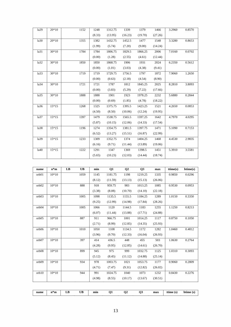
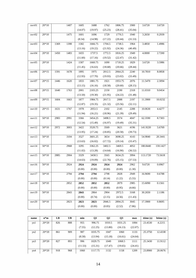
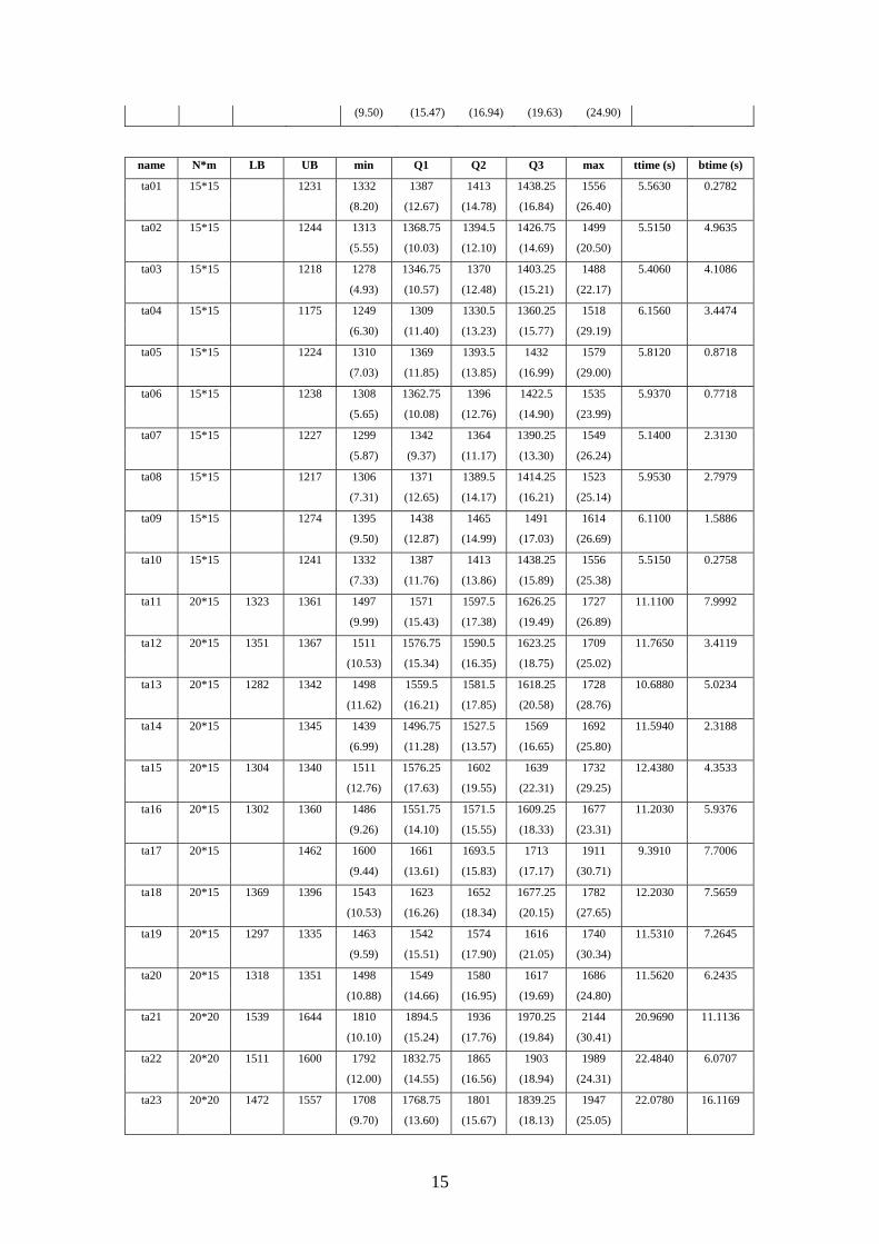
The tables have the following structure: in each line it is presented the name of the

instance, the number of jobs and the number of machines of the instance )*( mn , and

the best lower and upper bound values (LB, UB) of the makespan. If the lower bound

is omitted, the upper bound is optimal. We gathered the values of these bounds from

the paper of Jain and Meeran (1999) and the papers of Nowicki and Smutnicki (1996;

2002 and 2005).

The algorithm has been run 100 times for each instance on a Pentium 4 CPU 2.80

GHz and coded in C. The tables also present some statistical values concerning the

11

makespan of the solutions found in the 100 runs, as well as the total time of all runs

(ttime) and the time to the best solution found (btime), in seconds. The statistics of the

makespan computed over the 100 runs are the minimum (min), the first quartile (Q1),

the median (Q2), the third quartile (Q3) and the maximum (max). We chose this

measures because they allow us to see how disperse are the values obtain by different

runs, which give us an idea of the robustness of the algorithm. Within brackets, next

to each value , is the correspondent percentage of relative error to the upperbound:

( ) ( )UB

UBxfxREUB−

×= %100

Whenever the values are not worse than the best known upper bound, we present

them in bold. Although this is a very simple (and fast) algorithm, it happens in 23 of

the 152 instances used in this study.

name n*m LB UB min Q1 Q2 Q3 max ttime (s) btime(s)

abz5 10*10 1234 1258 1312 1332 1358 1460 0.7650 0.0995

(1.94) (6.32) (7.94) (10.05) (18.31)

abz6 10*10 943 952 978.75 997 1012.5 1078 0.7660 0.3064

(0.95) (3.79) (5.73) (7.37) (14.32)

abz7 15*20 656 725 750.75 763 781 810 10.9070 3.4902

(10.52) (14.44) (16.31) (19.05) (23.48)

abz8 15*20 647 669 734 767 780 797.25 837 10.5160 1.8929

(9.72) (14.65) (16.59) (19.17) (25.11)

abz9 15*20 661 679 754 782.5 792 809 874 10.4690 1.3610

(11.05) (15.24) (16.64) (19.15) (28.72)

name n*m LB UB min Q1 Q2 Q3 max ttime

(s)

btime(s

)

ft06 6*6 55 55 59 59 61 66 0.1400 0.1274

(0.00) (7.27) (7.27) (10.91) (20.00)

ft10 10*10 930 970 1026.75 1046 1073.25 1144 1.0000 0.5800

(4.30) (10.40) (12.47) (15.40) (23.01)

ft20 20*5 1165 1283 1304 1318 1365 1409 0.4690 0.0094

(10.13) (11.93) (13.13) (17.17) (20.94)

name n*m LB UB min Q1 Q2 Q3 max ttime(s) btime(s)

la01 10*5 666 666 666 666 666 694 0.1720 0.0017

(0.00) (0.00) (0.00) (0.00) (4.20)

la02 10*5 655 667 712 722 722 835 0.1560 0.0437

(1.83) (8.70) (10.23) (10.23) (27.48)

la03 10*5 597 605 605 640 701 701 0.2190 0.0066

(1.34) (1.34) (7.20) (17.42) (17.42)

la04 10*5 590 607 610 648 648 672 0.1710 0.0051

12

(2.88) (3.39) (9.83) (9.83) (13.90)

la05 10*5 593 593 593 593 593 593 0.1100 0.0011

(0.00) (0.00) (0.00) (0.00) (0.00)

la06 15*5 926 926 926 926 926 926 0.1710 0.0017

(0.00) (0.00) (0.00) (0.00) (0.00)

la07 15*5 890 890 890 890 890 936 0.2030 0.0020

(0.00) (0.00) (0.00) (0.00) (5.17)

la08 15*5 863 863 863 880 921 976 0.2970 0.0149

(0.00) (0.00) (1.97) (6.72) (13.09)

la09 15*5 951 951 951 951 951 953 0.2810 0.0028

(0.00) (0.00) (0.00) (0.00) (0.21)

la10 15*5 958 958 958 958 958 958 0.1410 0.0014

(0.00) (0.00) (0.00) (0.00) (0.00)

la11 20*5 1222 1222 1222 1222 1222 1284 0.2660 0.0027

(0.00) (0.00) (0.00) (0.00) (5.07)

la12 20*5 1039 1039 1039 1039 1039 1039 0.2650 0.0027

(0.00) (0.00) (0.00) (0.00) (0.00)

la13 20*5 1150 1150 1150 1150 1150 1223 0.3750 0.0038

(0.00) (0.00) (0.00) (0.00) (6.35)

la14 20*5 1292 1292 1292 1292 1292 1292 0.2180 0.0022

(0.00) (0.00) (0.00) (0.00) (0.00)

la15 20*5 1207 1207 1240 1295 1295 1295 0.9060 0.0453

(0.00) (2.73) (7.29) (7.29) (7.29)

la16 10*10 945 1012 1038.5 1049 1060 1099 0.7350 0.0221

(7.09) (9.89) (11.01) (12.17) (16.30)

la17 10*10 784 787 813.75 836.5 864.25 950 0.7660 0.0843

(0.38) (3.79) (6.70) (10.24) (21.17)

la18 10*10 848 854 879.25 895 924 1042 0.7500 0.3000

(0.71) (3.69) (5.54) (8.96) (22.88)

la19 10*10 842 861 893.75 917 940.5 1020 0.9690 0.4554

(2.26) (6.15) (8.91) (11.70) (21.14)

la20 10*10 902 920 960 976 1011.5 1080 0.8130 0.0813

(2.00) (6.43) (8.20) (12.14) (19.73)

la21 15*10 1046 1092 1154 1177.5 1210.25 1286 2.0460 0.1023

(4.40) (10.33) (12.57) (15.70) (22.94)

la22 15*10 927 955 999 1029.5 1063.5 1192 1.7970 0.9884

(3.02) (7.77) (11.06) (14.72) (28.59)

la23 15*10 1032 1049 1089.25 1111 1136 1268 1.8900 1.7388

(1.65) (5.55) (7.66) (10.08) (22.87)

la24 15*10 935 971 1016 1030 1054.25 1104 1.8440 0.6270

(3.85) (8.66) (10.16) (12.75) (18.07)

la25 15*10 977 1027 1082.75 1100 1122.25 1226 1.7960 0.5388

(5.12) (10.82) (12.59) (14.87) (25.49)

la26 20*10 1218 1265 1321.75 1355 1376 1485 3.3750 3.0375

(3.86) (8.52) (11.25) (12.97) (21.92)

la27 20*10 1235 1308 1375 1399 1431.25 1538 3.5620 0.1781

(5.91) (11.34) (13.28) (15.89) (24.53)

la28 20*10 1216 1301 1360.75 1391 1413.25 1533 3.0000 0.1500

(6.99) (11.90) (14.39) (16.22) (26.07)

13

la29 20*10 1152 1248 1312.75 1339 1379 1466 3.2960 0.8570

(8.33) (13.95) (16.23) (19.70) (27.26)

la30 20*10 1355 1382 1432.75 1452.5 1477 1548 3.3280 0.8653

(1.99) (5.74) (7.20) (9.00) (14.24)

la31 30*10 1784 1784 1806.75 1829.5 1866.25 2006 7.0160 0.0702

(0.00) (1.28) (2.55) (4.61) (12.44)

la32 30*10 1850 1850 1868.75 1906 1931 2024 6.2350 0.5612

(0.00) (1.01) (3.03) (4.38) (9.41)

la33 30*10 1719 1719 1729.75 1756.5 1797 1872 7.9060 1.2650

(0.00) (0.63) (2.18) (4.54) (8.90)

la34 30*10 1721 1721 1787 1812 1845.25 2025 8.2810 3.8093

(0.00) (3.83) (5.29) (7.22) (17.66)

la35 30*10 1888 1888 1901 1923 1978.25 2232 5.6880 0.2844

(0.00) (0.69) (1.85) (4.78) (18.22)

la36 15*15 1268 1325 1375.75 1395.5 1423.25 1521 4.2650 0.0853

(4.50) (8.50) (10.06) (12.24) (19.95)

la37 15*15 1397 1479 1538.75 1565.5 1597.25 1642 4.7970 4.0295

(5.87) (10.15) (12.06) (14.33) (17.54)

la38 15*15 1196 1274 1354.75 1381.5 1397.75 1471 5.1090 0.7153

(6.52) (13.27) (15.51) (16.87) (22.99)

la39 15*15 1233 1309 1352.75 1374 1404.25 1468 4.4530 2.9835

(6.16) (9.71) (11.44) (13.89) (19.06)

la40 15*15 1222 1291 1347 1369 1398.5 1451 5.3910 3.5581

(5.65) (10.23) (12.03) (14.44) (18.74)

name n*m LB UB min Q1 Q2 Q3 max ttime(s) btime(s)

orb01 10*10 1059 1145 1181.75 1198 1219.25 1335 0.9850 0.0296

(8.12) (11.59) (13.13) (15.13) (26.06)

orb02 10*10 888 918 959.75 983 1013.25 1085 0.9530 0.0953

(3.38) (8.08) (10.70) (14.10) (22.18)

orb03 10*10 1005 1098 1135.5 1155.5 1184.25 1289 1.0150 0.3350

(9.25) (12.99) (14.98) (17.84) (28.26)

orb04 10*10 1005 1066 1120 1144.5 1183 1255 1.1250 0.8213

(6.07) (11.44) (13.88) (17.71) (24.88)

orb05 10*10 887 911 966.75 1001 1014.25 1117 0.8750 0.1050

(2.71) (8.99) (12.85) (14.35) (25.93)

orb06 10*10 1010 1050 1108 1134.5 1172 1282 1.0460 0.4812

(3.96) (9.70) (12.33) (16.04) (26.93)

orb07 10*10 397 414 436.5 448 455 503 1.0630 0.2764

(4.28) (9.95) (12.85) (14.61) (26.70)

orb08 10*10 899 945 975 999 1032.75 1125 1.0310 0.3093

(5.12) (8.45) (11.12) (14.88) (25.14)

orb09 10*10 934 978 1003.75 1021 1053.75 1177 0.9060 0.2809

(4.71) (7.47) (9.31) (12.82) (26.02)

orb10 10*10 944 991 1024.75 1040 1073 1232 0.8430 0.2276

(4.98) (8.55) (10.17) (13.67) (30.51)

name n*m LB UB min Q1 Q2 Q3 max ttime (s) btime (s)

14

swv01 20*10 1407 1605 1688 1762 1806.75 1900 3.6720 3.6720

(14.07) (19.97) (25.23) (28.41) (35.04)

swv02 20*10 1475 1601 1696 1729 1776.5 1940 3.2650 0.2939

(8.54) (14.98) (17.22) (20.44) (31.53)

swv03 20*10 1369 1398 1582 1666.75 1704.5 1738.5 1964 3.4850 1.4986

(13.16) (19.22) (21.92) (24.36) (40.49)

swv04 20*10 1450 1483 1655 1737.5 1772.5 1816.25 1949 4.0000 2.7200

(11.60) (17.16) (19.52) (22.47) (31.42)

swv05 20*10 1424 1587 1660.75 1690 1718.25 1829 3.6720 3.5986

(11.45) (16.63) (18.68) (20.66) (28.44)

swv06 20*15 1591 1678 1895 1975 2012.5 2064.25 2240 10.7810 8.0858

(12.93) (17.70) (19.93) (23.02) (33.49)

swv07 20*15 1446 1620 1833 1881.75 1921 1953.75 2076 11.5470 2.3094

(13.15) (16.16) (18.58) (20.60) (28.15)

swv08 20*15 1640 1763 2001 2103.25 2150 2190 2318 11.0310 9.0454

(13.50) (19.30) (21.95) (24.22) (31.48)

swv09 20*15 1604 1663 1877 1984.75 2017.5 2088 2197 11.3900 10.0232

(12.87) (19.35) (21.32) (25.56) (32.11)

swv10 20*15 1631 1767 1978 2053.5 2102 2145 2288 10.0630 4.4277

(11.94) (16.21) (18.96) (21.39) (29.49)

swv11 50*10 2983 2991 3366 3454.25 3498.5 3574 4047 62.3590 8.7303

(12.54) (15.49) (16.97) (19.49) (35.31)

swv12 50*10 2972 3003 3422 3520.75 3569 3621 4196 141.9220 5.6769

(13.95) (17.24) (18.85) (20.58) (39.73)

swv13 50*10 3104 3527 3601.25 3654 3698.25 4143 54.9840 20.3441

(13.63) (16.02) (17.72) (19.14) (33.47)

swv14 50*10 2968 3295 3362.25 3402.5 3469.5 4052 180.8440 159.1427

(11.02) (13.28) (14.64) (16.90) (36.52)

swv15 50*10 2885 2904 3329 3458.5 3565 3634.25 3994 113.1720 73.5618

(14.63) (19.09) (22.76) (25.15) (37.53)

swv16 50*10 2924 2924 2924 2924 2924 2962 9.6720 0.0967

(0.00) (0.00) (0.00) (0.00) (1.30)

swv17 50*10 2794 2794 2794 2798 2828 2949 16.9690 0.6788

(0.00) (0.00) (0.14) (1.22) (5.55)

swv18 50*10 2852 2852 2852 2852 2879 2985 15.6090 0.1561

(0.00) (0.00) (0.00) (0.95) (4.66)

swv19 50*10 2843 2843 2864 2904 2972.5 3168 30.2650 2.1186

(0.00) (0.74) (2.15) (4.56) (11.43)

swv20 50*10 2823 2823 2823 2846.5 2894.25 3045 17.3900 0.8695

(0.00) (0.00) (0.83) (2.52) (7.86)

name n*m LB UB min Q1 Q2 Q3 max ttime (s) btime (s)

yn1 20*20 826 888 955 996.75 1010.5 1031.25 1084 23.4530 4.2215

(7.55) (12.25) (13.80) (16.13) (22.07)

yn2 20*20 861 909 987 1035.75 1047 1060 1133 25.3750 12.4338

(8.58) (13.94) (15.18) (16.61) (24.64)

yn3 20*20 827 893 996 1029.75 1049 1068.5 1111 25.3430 11.9112

(11.53) (15.31) (17.47) (19.65) (24.41)

yn4 20*20 918 968 1060 1117.75 1132 1158 1209 23.8900 20.0676

15

(9.50) (15.47) (16.94) (19.63) (24.90)

name N*m LB UB min Q1 Q2 Q3 max ttime (s) btime (s)

ta01 15*15 1231 1332 1387 1413 1438.25 1556 5.5630 0.2782

(8.20) (12.67) (14.78) (16.84) (26.40)

ta02 15*15 1244 1313 1368.75 1394.5 1426.75 1499 5.5150 4.9635

(5.55) (10.03) (12.10) (14.69) (20.50)

ta03 15*15 1218 1278 1346.75 1370 1403.25 1488 5.4060 4.1086

(4.93) (10.57) (12.48) (15.21) (22.17)

ta04 15*15 1175 1249 1309 1330.5 1360.25 1518 6.1560 3.4474

(6.30) (11.40) (13.23) (15.77) (29.19)

ta05 15*15 1224 1310 1369 1393.5 1432 1579 5.8120 0.8718

(7.03) (11.85) (13.85) (16.99) (29.00)

ta06 15*15 1238 1308 1362.75 1396 1422.5 1535 5.9370 0.7718

(5.65) (10.08) (12.76) (14.90) (23.99)

ta07 15*15 1227 1299 1342 1364 1390.25 1549 5.1400 2.3130

(5.87) (9.37) (11.17) (13.30) (26.24)

ta08 15*15 1217 1306 1371 1389.5 1414.25 1523 5.9530 2.7979

(7.31) (12.65) (14.17) (16.21) (25.14)

ta09 15*15 1274 1395 1438 1465 1491 1614 6.1100 1.5886

(9.50) (12.87) (14.99) (17.03) (26.69)

ta10 15*15 1241 1332 1387 1413 1438.25 1556 5.5150 0.2758

(7.33) (11.76) (13.86) (15.89) (25.38)

ta11 20*15 1323 1361 1497 1571 1597.5 1626.25 1727 11.1100 7.9992

(9.99) (15.43) (17.38) (19.49) (26.89)

ta12 20*15 1351 1367 1511 1576.75 1590.5 1623.25 1709 11.7650 3.4119

(10.53) (15.34) (16.35) (18.75) (25.02)

ta13 20*15 1282 1342 1498 1559.5 1581.5 1618.25 1728 10.6880 5.0234

(11.62) (16.21) (17.85) (20.58) (28.76)

ta14 20*15 1345 1439 1496.75 1527.5 1569 1692 11.5940 2.3188

(6.99) (11.28) (13.57) (16.65) (25.80)

ta15 20*15 1304 1340 1511 1576.25 1602 1639 1732 12.4380 4.3533

(12.76) (17.63) (19.55) (22.31) (29.25)

ta16 20*15 1302 1360 1486 1551.75 1571.5 1609.25 1677 11.2030 5.9376

(9.26) (14.10) (15.55) (18.33) (23.31)

ta17 20*15 1462 1600 1661 1693.5 1713 1911 9.3910 7.7006

(9.44) (13.61) (15.83) (17.17) (30.71)

ta18 20*15 1369 1396 1543 1623 1652 1677.25 1782 12.2030 7.5659

(10.53) (16.26) (18.34) (20.15) (27.65)

ta19 20*15 1297 1335 1463 1542 1574 1616 1740 11.5310 7.2645

(9.59) (15.51) (17.90) (21.05) (30.34)

ta20 20*15 1318 1351 1498 1549 1580 1617 1686 11.5620 6.2435

(10.88) (14.66) (16.95) (19.69) (24.80)

ta21 20*20 1539 1644 1810 1894.5 1936 1970.25 2144 20.9690 11.1136

(10.10) (15.24) (17.76) (19.84) (30.41)

ta22 20*20 1511 1600 1792 1832.75 1865 1903 1989 22.4840 6.0707

(12.00) (14.55) (16.56) (18.94) (24.31)

ta23 20*20 1472 1557 1708 1768.75 1801 1839.25 1947 22.0780 16.1169

(9.70) (13.60) (15.67) (18.13) (25.05)

16

ta24 20*20 1602 1647 1778 1864.75 1894.5 1925.25 2014 19.1870 17.0764

(7.95) (13.22) (15.03) (16.89) (22.28)

ta25 20*20 1504 1595 1746 1830.75 1876 1913.5 1992 20.4060 16.1207

(9.47) (14.78) (17.62) (19.97) (24.89)

ta26 20*20 1539 1645 1768 1863.75 1907 1950.25 2027 17.8440 2.6766

(7.48) (13.30) (15.93) (18.56) (23.22)

ta27 20*20 1616 1680 1839 1923.75 1954 1988.25 2149 19.8440 17.8596

(9.46) (14.51) (16.31) (18.35) (27.92)

ta28 20*20 1591 1614 1755 1837.5 1871 1908.75 2016 22.3130 19.1892

(8.74) (13.85) (15.92) (18.26) (24.91)

ta29 20*20 1514 1625 1717 1835.75 1864 1898.25 2012 20.1570 6.2487

(5.66) (12.97) (14.71) (16.82) (23.82)

ta30 20*20 1473 1584 1737 1800.75 1827.5 1852.5 1960 17.5470 6.4924

(9.66) (13.68) (15.37) (16.95) (23.74)

ta31 30*15 1764 1976 2059.75 2099.5 2135 2322 30.6090 14.3862

(12.02) (16.77) (19.02) (21.03) (31.63)

ta32 30*15 1774 1796 2029 2132.5 2165.5 2205 2356 30.6090 23.8750

(12.97) (18.74) (20.57) (22.77) (31.18)

ta33 30*15 1778 1793 2070 2171.25 2204 2265 2336 31.9220 18.1955

(15.45) (21.10) (22.92) (26.32) (30.28)

ta34 30*15 1828 1829 2024 2114.25 2156 2186 2287 33.6720 32.3251

(10.66) (15.60) (17.88) (19.52) (25.04)

ta35 30*15 2007 2093 2174.25 2208 2250.25 2454 35.2970 13.4129

(4.29) (8.33) (10.01) (12.12) (22.27)

ta36 30*15 1819 2040 2124.5 2153.5 2204.25 2307 30.5310 3.9690

(12.15) (16.79) (18.39) (21.18) (26.83)

ta37 30*15 1771 1778 1967 2099.75 2136 2184.5 2408 29.0310 15.3864

(10.63) (18.10) (20.13) (22.86) (35.43)

ta38 30*15 1673 1913 1976.75 2003.5 2046.25 2188 34.0000 12.5800

(14.35) (18.16) (19.75) (22.31) (30.78)

ta39 30*15 1795 1966 2069.25 2107.5 2144 2321 31.3750 13.4913

(9.53) (15.28) (17.41) (19.44) (29.30)

ta40 30*15 1631 1674 1931 2012 2047.5 2077.25 2218 33.9850 0.3399

(15.35) (20.19) (22.31) (24.09) (32.50)

ta41 30*20 1859 2018 2348 2413.75 2458 2494 2638 61.1100 0.6111

(16.35) (19.61) (21.80) (23.59) (30.72)

ta42 30*20 1867 1956 2206 2301.75 2341 2374.25 2513 62.3280 49.2391

(12.78) (17.68) (19.68) (21.38) (28.48)

ta43 30*20 1809 1859 2155 2228.5 2254 2294.5 2395 72.7040 50.8928

(15.92) (19.88) (21.25) (23.43) (28.83)

ta44 30*20 1927 1984 2300 2382.5 2418 2466 2577 64.7970 11.6635

(15.93) (20.09) (21.88) (24.29) (29.89)

ta45 30*20 1997 2000 2295 2358 2380 2410.25 2581 70.8280 34.7057

(14.75) (17.90) (19.00) (20.51) (29.05)

ta46 30*20 1940 2021 2314 2399.5 2438 2481 2660 64.1090 25.6436

(14.50) (18.73) (20.63) (22.76) (31.62)

ta47 30*20 1789 1903 2151 2260.5 2299.5 2345.75 2443 63.9850 63.3452

(13.03) (18.79) (20.84) (23.27) (28.38)

ta48 30*20 1912 1952 2222 2325.5 2360 2407.5 2565 63.2190 60.0581

17

(13.83) (19.13) (20.90) (23.34) (31.40)

ta49 30*20 1915 1968 2250 2349.5 2390 2425 2560 65.2650 11.7477

(14.33) (19.39) (21.44) (23.22) (30.08)

ta50 30*20 1807 1928 2264 2347.5 2387 2431 2633 63.2970 13.2924

(17.43) (21.76) (23.81) (26.09) (36.57)

ta51 50*15 2760 3001 3149 3227 3294 3587 139.8750 65.7413

(8.73) (14.09) (16.92) (19.35) (29.96)

ta52 50*15 2756 2940 3136 3216 3276.5 3590 128.3590 119.3739

(6.68) (13.79) (16.69) (18.89) (30.26)

ta53 50*15 2717 2895 2998 3031.5 3072.5 3219 116.9370 87.7028

(6.55) (10.34) (11.58) (13.08) (18.48)

ta54 50*15 2839 2914 3024.75 3092.5 3133.75 3280 112.5470 15.7566

(2.64) (6.54) (8.93) (10.38) (15.53)

ta55 50*15 2679 2988 3133 3178 3247.5 3440 144.6570 56.4162

(11.53) (16.95) (18.63) (21.22) (28.41)

ta56 50*15 2781 2966 3122.75 3167 3230.25 3437 131.3750 3.9413

(6.65) (12.29) (13.88) (16.15) (23.59)

ta57 50*15 2943 3101 3213.5 3256.5 3320.5 3485 106.4220 27.6697

(5.37) (9.19) (10.65) (12.83) (18.42)

ta58 50*15 2885 3103 3214.5 3273 3326.25 3438 146.9060 104.3033

(7.56) (11.42) (13.45) (15.29) (19.17)

ta59 50*15 2655 2940 3038.25 3090 3139.5 3294 124.2970 119.3251

(10.73) (14.44) (16.38) (18.25) (24.07)

ta60 50*15 2723 2921 3048.5 3104 3160 3339 121.7970 86.4759

(7.27) (11.95) (13.99) (16.05) (22.62)

ta61 50*20 2868 3258 3369.5 3424 3484 3649 285.5000 216.9800

(13.60) (17.49) (19.39) (21.48) (27.23)

ta62 50*20 2869 2872 3306 3444 3493.5 3544 3730 311.9850 293.2659

(15.11) (19.92) (21.64) (23.40) (29.87)

ta63 50*20 2755 3130 3218.75 3273 3324.25 3487 315.1250 302.5200

(13.61) (16.83) (18.80) (20.66) (26.57)

ta64 50*20 2702 3008 3180.25 3230 3287.75 3431 289.8440 153.6173

(11.32) (17.70) (19.54) (21.68) (26.98)

ta65 50*20 2725 3104 3242.5 3286 3339 3569 323.2340 42.0204

(13.91) (18.99) (20.59) (22.53) (30.97)

ta66 50*20 2845 3198 3320 3361 3415.5 3585 317.1570 63.4314

(12.41) (16.70) (18.14) (20.05) (26.01)

ta67 50*20 2825 3209 3339 3389.5 3435.25 3578 273.3440 46.4685

(13.59) (18.19) (19.98) (21.60) (26.65)

ta68 50*20 2784 3133 3235.75 3283 3337.5 3542 268.7810 223.0882

(12.54) (16.23) (17.92) (19.88) (27.23)

ta69 50*20 3071 3366 3447.5 3517 3576 3739 259.1720 33.6924

(9.61) (12.26) (14.52) (16.44) (21.75)

ta70 50*20 2995 3449 3528.75 3582 3633.25 3815 279.5150 58.6982

(15.16) (17.82) (19.60) (21.31) (27.38)

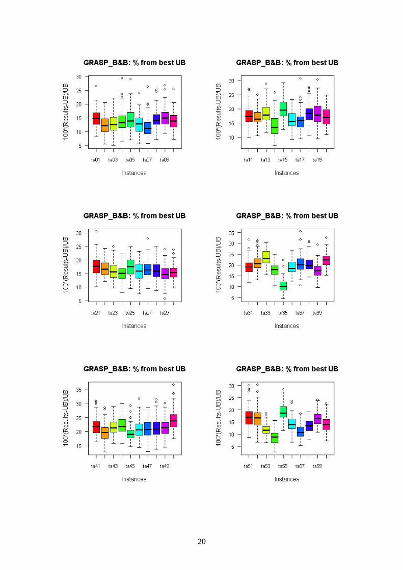
The information of these tables can be visualised using boxplots. They show that

the quality achieved is more dependent on the ratio mn / than on the absolute

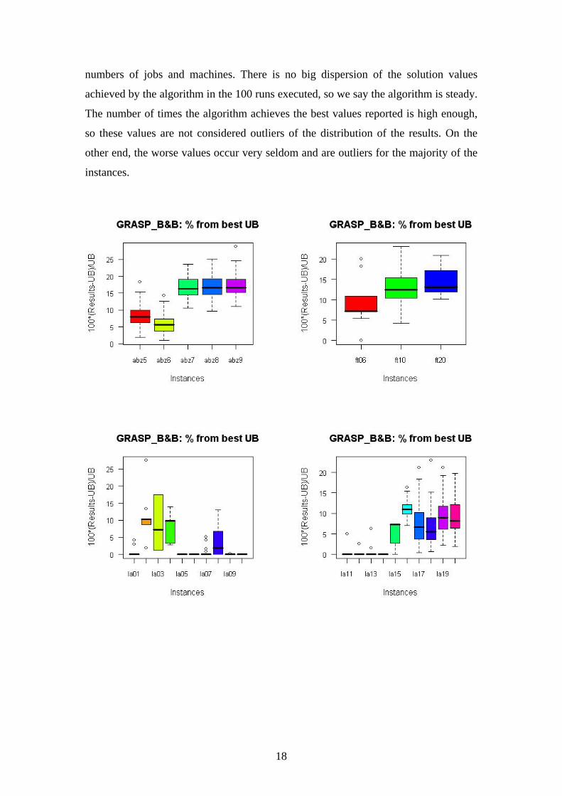
18

numbers of jobs and machines. There is no big dispersion of the solution values

achieved by the algorithm in the 100 runs executed, so we say the algorithm is steady.

The number of times the algorithm achieves the best values reported is high enough,

so these values are not considered outliers of the distribution of the results. On the

other end, the worse values occur very seldom and are outliers for the majority of the

instances.

19

20

21

5.1. Comparison to other procedures

GRASP_B&B OSH heuristic is a very simple GRASP algorithm with a

construction phase very similar to the one of the shifting bottleneck. Therefore, we

show comparative results to two other very similar methods: a simple GRASP

heuristic of Binato et al (2001) and the Shifting Bottleneck heuristic by Adams et al

(1988).

5.1.1. Comparison to GRASP of Binato et al (2001)

The GRASP heuristic by Binato et al (2001) has a different building step in the

construction phase, which consists in scheduling one operation at each step. In their

computational results, they present the time in seconds per thousand iterations (an

iteration is one building phase followed by a local search) and the thousands of

iterations. For a comparison purpose we multiply these values to get the total

computation time. For GRASP_B&B we present the total time of all runs (ttime), in

seconds. As the tables show, our algorithm is much faster. Whenever our GRASP

achieves a solution not worse than theirs, we present the respective value in bold. This

happens for 26 of the 58 instances whose results where compared.

name GRASP_B&B ttime (s) GRASP time (s)

abz5 1258 0.7650 1238 6030

abz6 952 0.7660 947 62310

abz7 725 10.9070 667 349740

abz8 734 10.5160 729 365820

22

abz9 754 10.4690 758 343710

name GRASP_B&B ttime (s) GRASP time (s)

ft06 55 0.1400 55 70

ft10 970 1.0000 938 261290

ft20 1283 0.4690 1169 387430

name GRASP_B&B ttime (s) GRASP time (s)

la01 666 0.1720 666 140

la02 667 0.1560 655 140

la03 605 0.2190 604 65130

la04 607 0.1710 590 130

la05 593 0.1100 593 130

la06 926 0.1710 926 240

la07 890 0.2030 890 250

la08 863 0.2970 863 240

la09 951 0.2810 951 290

la10 958 0.1410 958 250

la11 1222 0.2660 1222 410

la12 1039 0.2650 1039 390

la13 1150 0.3750 1150 430

la14 1292 0.2180 1292 390

la15 1207 0.9060 1207 410

la16 1012 0.7350 946 155310

la17 787 0.7660 784 60300

la18 854 0.7500 848 58290

la19 861 0.9690 842 31310

la20 920 0.8130 907 160320

la21 1092 2.0460 1091 325650

la22 955 1.7970 960 315630

la23 1049 1.8900 1032 65650

la24 971 1.8440 978 64640

la25 1027 1.7960 1028 64640

la26 1265 3.3750 1271 109080

la27 1308 3.5620 1320 110090

la28 1301 3.0000 1293 110090

la29 1248 3.2960 1293 112110

la30 1382 3.3280 1368 106050

la31 1784 7.0160 1784 231290

23

la32 1850 6.2350 1850 241390

la33 1719 7.9060 1719 241390

la34 1721 8.2810 1753 240380

la35 1888 5.6880 1888 222200

la36 1325 4.2650 1334 115360

la37 1479 4.7970 1457 115360

la38 1274 5.1090 1267 118720

la39 1309 4.4530 1290 115360

la40 1291 5.3910 1259 123200

name GRASP_B&B ttime (s) GRASP time (s)

orb01 1145 0.9850 1070 116290

orb02 918 0.9530 889 152380

orb03 1098 1.0150 1021 124310

orb04 1066 1.1250 1031 124310

orb05 911 0.8750 891 112280

orb06 1050 1.0460 1013 124310

orb07 414 1.0630 397 128320

orb08 945 1.0310 909 124310

orb09 978 0.9060 945 124310

orb10 991 0.8430 953 116290

5.1.2. Comparison to the Shifting Bottleneck (Adams et al. 1988)

The main difference of the Shifting Bottleneck procedure (Adams et al. 1988) and

GRASP_B&B is the random selection of the machine to be scheduled. In the Shifting

Bottleneck the machine to be scheduled is always the bottleneck machine. The

comparison between the shifting bottleneck procedure (Adams et al. 1988) and the

GRASP_B&B is also presented next. Comparing the computation times of both

procedures, the GRASP_B&B is slightly faster than the shifting bottleneck for smaller

instances. Given the distinct computers used in the experiments we would say that this

is not meaningful, but the difference does get accentuated as the dimensions grow.

Whenever GRASP_B&B achieves a solution better than the shifting bottleneck

procedure, we present its value in bold. This happens in 29 of the 48 instances whose

results where compared, and in 16 of the remaining 19 instances the best value found

was the same.

24

name GRASP_B&B ttime (s) Shifting

Bottleneck

time (s)

abz5 1258 0.7650 1306 5.7

abz6 952 0.7660 962 12.67

abz7 725 10.9070 730 118.87

abz8 734 10.5160 774 125.02

abz9 754 10.4690 751 94.32

name GRASP_B&B ttime (s) Shifting

Bottleneck

time (s)

ft06 55 0.1400 55 1.5

ft10 970 1.0000 1015 10.1

ft20 1283 0.4690 1290 3.5

name GRASP_B&B ttime (s) Shifting

Bottleneck

time (s)

la01 666 0.1720 666 1.26

la02 667 0.1560 720 1.69

la03 605 0.2190 623 2.46

la04 607 0.1710 597 2.79

la05 593 0.1100 593 0.52

la06 926 0.1710 926 1.28

la07 890 0.2030 890 1.51

la08 863 0.2970 868 2.41

la09 95º1 0.2810 951 0.85

la10 958 0.1410 959 0.81

la11 1222 0.2660 1222 2.03

la12 1039 0.2650 1039 0.87

la13 1150 0.3750 1150 1.23

la14 1292 0.2180 1292 0.94

la15 1207 0.9060 1207 3.09

la16 1012 0.7350 1021 6.48

la17 787 0.7660 796 4.58

la18 854 0.7500 891 10.2

la19 861 0.9690 875 7.4

la20 920 0.8130 924 10.2

la21 1092 2.0460 1172 21.9

la22 955 1.7970 1040 19.2

la23 1049 1.8900 1061 24.6

25

la24 971 1.8440 1000 25.5

la25 1027 1.7960 1048 27.9

la26 1265 3.3750 1304 48.5

la27 1308 3.5620 1325 45.5

la28 1301 3.0000 1256 28.5

la29 1248 3.2960 1294 48

la30 1382 3.3280 1403 37.8

la31 1784 7.0160 1784 38.3

la32 1850 6.2350 1850 29.1

la33 1719 7.9060 1719 25.6

la34 1721 8.2810 1721 27.6

la35 1888 5.6880 1888 21.3

la36 1325 4.2650 1351 46.9

la37 1479 4.7970 1485 6104

la38 1274 5.1090 1280 57.5

la39 1309 4.4530 1321 71.8

la40 1291 5.3910 1326 76.7

6. Conclusions

In this work we present a very simple Optimized Search Heuristic, the

GRASP_B&B to solve the Job-Shop Scheduling problem. This method is intended to

be a starting point for a more elaborated metaheuristic, since it obtains reasonable

solutions in very short running times. The main idea behind the GRASP_B&B

heuristic is to insert in each iteration of the building phase of the GRASP method the

complete solution of one-machine scheduling problems solved by a branch-an-bound

method, instead of insert one sequence of two individual operations as it is usual in

other GRASP methods for this problem.

We have compared it with other similar methods also used as an initialization

phase within more complex algorithms; namely a GRASP of Binato et. al (2001),

which is the base for a GRASP with path-relinking procedure of Aiex et. al (2003),

and the Shifting Bottleneck procedure of Adams et. al (1988), incorporated in the

successful guided local search of Balas and Vazacopoulos (1991). The comparison to

the GRASP of Binato et al (2001) shows that the GRASP_B&B is much faster than

theirs. The quality of their best solution is slightly better than ours in 60% of the

instances tested. When comparing GRASP_B&B with the Shifting Bottleneck, the

first one is still faster, and it achieves better solutions, except for 3 of the comparable

26

instances. Therefore we can conclude, that the GRASP_B&B is a good method to use

as the initialization phase of more elaborated and complex methods to solve the job-

shop scheduling problem. As future research, we are working on this elaborated

method also using OSH ideas, i.e. combing heuristic and exact methods procedures.

Acknowledgement

Susana Fernandes’ work is suported by the the programm POCI2010 of the

Portuguese Fundação para a Ciência e Tecnologia. Helena R. Lourenço’s work is

supported by Ministerio de Educación y Ciencia, Spain, SEC2003-01991/ECO.

References

1 Adams, J., E. Balas and D. Zawack (1988). "The Shifting Bottleneck Procedure for

Job Shop Scheduling." Management Science, vol. 34(3): pp. 391-401.

2 Applegate, D. and W. Cook (1991). "A Computational Study of the Job-Shop

Scheduling Problem." ORSA Journal on Computing, vol. 3(2): pp. 149-156.

3 Balas, E. and A. Vazacopoulos (1998). "Guided Local Search with Shifting

Bottleneck for Job Shop Scheduling." Management Science, vol. 44(2): pp. 262-

275.

4 Binato, S., W. J. Hery, D. M. Loewenstern and M. G. C. Resende (2001). "A

GRASP for Job Shop Scheduling." In C.C. Ribeiro and P. Hansen, editors, Essays

and surveys on metaheuristics, pp. 59-79. Kluwer Academic Publishers.

5 Carlier, J. (1982). "The one-machine sequencing problem." European Journal of

Operational Research, vol. 11: pp. 42-47.

6 Caseau, Y. and F. Laburthe (1995), "Disjunctive scheduling with task intervals",

Technical Report LIENS, 95-25, Ecole Normale Superieure Paris.

7 Chen, S., S. Talukdar and N. Sadeh (1993). "Job-shop-scheduling by a team of

asynchronous agentes", Proceedings of the IJCAI-93 Workshop on Knowledge-

Based Production, Scheduling and Control. Chambery France.

8 Danna, E., E. Rothberg and C. L. Pape (2005). "Exploring relaxation induced

neighborhoods to improve MIP solutions." Mathematical Programming, Ser. A, vol.

102: pp. 71-90.

9 Dell'Amico, M. and M. Trubian (1993). "Applying Tabu-Search to the Job-Shop

Scheduling Problem."

27

10 Denzinger, J. and T. Offermann (1999). "On Cooperation between Evolutionary

Algorithms and other Search Paradigms", Proceedings of the 1999 Congress on

Evolutionary Computational.

11 Feo, T. and M. Resende (1995). "Greedy Randomized Adaptive Search

Procedures." Journal of Global Optimization, vol. 6: pp. 109-133.

12 Fernandes, S. and H.R. Lourenço (2007), "Optimized Search Heuristics",

Universitat Pompeu Fabra, Barcelona, Spain.

(http://www.econ.upf.edu/~ramalhin/OSHwebpage/index.html)

13 Fisher, H. and G. L. Thompson (1963). Probabilistic learning combinations of

local job-shop scheduling rules. In J. F. Muth and G. L. Thompson eds. Industrial

Scheduling. pp. 225-251. Prentice Hall, Englewood Cliffs.

14 Garey, M. R. and D. S. Johnson (1979). Computers and Intractability: A Guide to

the Theory of NP-Completeness. San Francisco, Freeman.

15 Jain, A. S. and S. Meeran (1999). "Deterministic job shop scheduling: Past, present

and future." European Journal of Operational Research, vol. 133: pp. 390-434.

16 Lawrence, S. (1984), "Resource Constrained Project Scheduling: an Experimental

Investigation of Heuristic Scheduling techniques", Graduate School of Industrial

Administration, Carnegie-Mellon University.

17 Lourenço, H. R. (1995). "Job-shop scheduling: Computational study of local

search and large-step optimization methods." European Journal of Operational

Research, vol. 83: pp. 347-367.

18 Lourenço, H. R. and M. Zwijnenburg (1996). Combining large-step optimization

with tabu-search: Application to the job-shop scheduling problem. In I. H. Osman

and J. P. Kelly eds. Meta-heuristics: Theory & Applications. Kluwer Academic

Publishers.

19 Nowicki, E. and C. Smutnicki (2002), "Some new tools to solve the job shop

problem", Technical Report, 60/2002, Institute of Engineering Cybernetics,

Wroclaw University of Technology.

20 Nowicki, E. and C. Smutnicki (2005). "An Advanced Tabu Search Algorithm for

the Job Shop Problem." Journal of Scheduling, vol. 8: pp. 145-159.

21 Nowicki, E. and C. Smutniki (1996). "A Fast Taboo Search Algorithm for the Job

Shop Problem." Management Science, vol. 42(6): pp. 797-813.

22 Roy, B. and B. Sussman (1964), "Les probèms d'ordonnancement avec

constraintes disjonctives", Note DS 9 bis, SEMA, Paris.

28

23 Schaal, A., A. Fadil, H. M. Silti and P. Tolla (1999). "Meta heuristics

diversification of generalized job shop scheduling based upon mathematical

programming techniques", Proceedings of the Cp-ai-or'99.

24 Schrage, L. (1970). "Solving resource-constrained network problems by implicit

enumeration: Non pre-emptive case." Operations Research, vol. 18: pp. 263-278.

25 Storer, R. H., S. D. Wu and R. Vaccari (1992). "New search spaces for sequencing

problems with application to job shop scheduling." Management Science, vol.

38(10): pp. 1495-1509.

26 Taillard, E. D. (1993). "Benchmarks for Basic Scheduling Problems." European

Journal of Operational Research, vol. 64(2): pp. 278-285.

27 Taillard, É. D. (1994). "Parallel Taboo Search Techniques for the Job Shop

Scheduling Problem." ORSA Journal on Computing, vol. 6(2): pp. 108-117.

28 Tamura, H., A. Hirahara, I. Hatono and M. Umano (1994). "An approximate

solution method for combinatorial optimisation." Transactions of the Society of

Instrument and Control Engineers, vol. 130: pp. 329-336.

29 Yamada, T. and R. Nakano (1992). A genetic algorithm applicable to large-scale

job-shop problems. In R. Manner and B. Manderick eds. Parallel Problem Solving

from Nature 2. pp. 281-290. Elsevier Science.