Neural Computation (accepted Nov 1, 2001) MS 2425

A Simple Model of Long-term Spike Train Regularization

Relly Brandman

Department of Computer Science and

Beckman Institute for Advanced Science and Technology,

University of Illinois, Urbana, Illinois 61801USA

Mark E. Nelson

Department of Molecular and Integrative Physiology and

Beckman Institute for Advanced Science and Technology,

University of Illinois, Urbana, Illinois 61801USA

Abstract: 335 words

Body: 6100 words (approx.)

Figures: 8

References: 21

Running title: Spike Train Regularization

Corresponding author information

address: Prof. Mark E. Nelson

Beckman Institute

University of Illinois

405 N. Mathews

Urbana, IL 61801

phone: (217)244-1371

fax: (217)244-5180

email: m-nelson@uiuc.edu

1

A Simple Model of Long-term Spike Train Regularization Relly Brandman Department of Computer Science and Beckman Institute for Advanced Science and Technology, University of Illinois, Urbana, Illinois 61801USA Mark E. Nelson Department of Molecular and Integrative Physiology and Beckman Institute for Advanced Science and Technology, University of Illinois, Urbana, Illinois 61801USA A simple model of spike generation is described that gives rise to negative correlations in the interspike interval (ISI) sequence and leads to long-term spike train regularization. This regularization can be seen by examining the variance of the kth-order interval distribution for large k (the times between spike i and spike i+k). The variance is much smaller than would be expected if successive ISIs were uncorrelated. Such regularizing effects have been observed in the spike trains of electrosensory afferent nerve fibers and can lead to dramatic improvement in the detectability of weak signals encoded in the spike train data (Ratnam & Nelson, 2000). Here we present a simple neural model in which negative ISI correlations and long-term spike train regularization arises from refractory effects associated with a dynamic spike threshold. Our model is derived from a more detailed model of electrosensory afferent dynamics developed recently by other investigators (Chacron, Longtin, St-Hilaire, & Maler, 2000; Chacron, Longtin, & Maler, 2001). The core of this model is a dynamic spike threshold that is transiently elevated following a spike, and subsequently decays until the next spike is generated. Here we present a simplified version–the linear adaptive threshold model–that contains a single state variable, and three free parameters that control the mean and coefficient of variation of the spontaneous ISI distribution and the frequency characteristics of the driven response. We show that refractory effects associated with the dynamic threshold lead to regularization of the spike train on long time scales. Furthermore, we show that this regularization enhances the detectability of weak signals encoded by the linear adaptive threshold model. Although inspired by properties of electrosensory afferent nerve fibers, such regularizing effects may play an important role in other neural systems where weak signals must be reliably detected in noisy spike trains. When modeling a neuronal system that exhibits this type of ISI correlation structure, the linear adaptive threshold model may provide a more appropriate starting point than conventional renewal process models that lack long-term regularizing effects.

2

1 Introduction When a spiking neuron encodes an input signal, subsequent processing of that signal by postsynaptic neurons must be based on changes in the statistical properties of the output spike train. If there is background spike activity, then the variability of the background will influence how reliably other neurons can detect the presence of a weak signal encoded in the spike train data. The variability of a spike train is often characterized by the coefficient of variation (CV) of the first-order interspike interval (ISI) distribution. However, the first-order ISI distribution provides information about variability only on short time scales comparable to the mean ISI (for review, see Gabbiani and Koch, 1998). It is possible for a spike train to be irregular on short time scales, but regular on longer time scales, as we have shown experimentally for P-type (probability-coding) electrosensory afferent nerve fibers in a weakly electric fish (Ratnam and Nelson, 2000). This longer-term regularization can be observed by analyzing the kth-order interval distribution (the distribution of time intervals between spike i and spike i+k). If successive ISIs in the spike train are uncorrelated, then the variance of the kth-order distribution will be a factor of k times larger than the variance of the first-order ISI distribution. However, in our experimental study of electrosensory afferents, we found that the variance between say every 50th spike in the spike train was significantly smaller than would be expected if successive ISIs were uncorrelated. We further demonstrated that this regularization is associated with negative correlations in the ISI sequence and that the detectability of a weak signal can be significantly enhanced when such regularization exists. The negative correlation structure and regularizing effects observed in the data have recently been reproduced in a modeling study based on a stochastic model of firing dynamics (Chacron et al., 2000; M. J. Chacron, A. Longtin, and L. Maler, 2001). Refractory effects are known to have a short-term regularizing influence on spike activity by decreasing the CV of the first-order ISI distribution and increasing the temporal precision of the driven response (Berry and Meister, 1998). Refractory effects are often modeled by introducing a recovery function that reduces the firing probability immediately following a spike (for reviews, see Berry and Meister, 1998; Johnson, 1996). In such models, refractory effects are dependent only on the time of the previous spike and are not sensitive to the duration of previous interspike intervals. If the input is held constant in such models, then successive intervals are independent and identically distributed. In this case no correlations are introduced into the ISI sequence. For such renewal models, the refractory mechanism has no impact on the long-term regularity of the spike train. In contrast, the refractory mechanism presented here is implemented as a dynamic state variable that retains a memory of previous activity spanning multiple interspike intervals. This non-renewal

3

model of spike generation gives rise to negative correlations in the ISI sequence and long-term regularization of the spike train. Here we present a simple model of a spike generating mechanism that gives rise to regularizing effects similar to those observed in electrosensory afferent spike trains. Our model is inspired by the more detailed model of Chacron et al. (2000; 2001), in which they showed that a stochastic model of spike generation with a dynamic threshold is able to accurately describe the key features of spike trains observed in the electrosensory afferent data (Nelson, Xu, & Payne, 1997; Ratnam & Nelson, 2000). To achieve a good match with the data, their model included about 15 parameters. However, because our model has only three parameters and one state variable, the relationships between the model parameters and the spike train properties are more readily apparent. Because of its simplicity, the model is easily adaptable to many neural modeling applications. In particular, it is a better choice than more widely used renewal process models when modeling spike trains that exhibit long-term regularizing effects. 2 The linear adaptive threshold model The goal of this simplified model is to obtain a minimal description of the spike generating mechanism that gives rise to long-term spike train regularization. This simplified model is intended to serve as a generic basis for constructing more detailed system-specific models, as illustrated by the example in Section 5. Although the model is highly simplified, it captures the important dynamic features of the process, and reflects a level of abstraction similar to that of the well-known integrate-and-fire model (Stein, 1967). An important simplification is that the model presented here uses a linear decay function, rather than the exponential threshold decay function used by Chacron et al. (2000; 2001). As we will show, this results in a simpler relationship between the model parameters and the spike train characteristics. Finally, the model presented here is formulated in a discrete-time framework, although it can also be cast in continuous time. A discrete-time formulation has the advantage of avoiding complications associated with the numerical integration of Gaussian noise in continuous time, and for this reason is more computationally efficient because it requires fewer integration steps per unit time. We are currently using an extended version of this model (see section 5) to simulate the neural activity of the entire population of 15,000 P-type electrosensory afferent nerve fibers of an electric fish, so matters of computational efficiency become of practical importance. The linear adaptive threshold model contains three essential parameters (a, b, and σ), and a single dynamic state variable, the spike threshold θ. For the sake of generality, we also include a fourth parameter c, the input gain, which we will subsequently take to be unity. As will be shown in Section 4, the parameter c is redundant in terms of

4

functionality, but it is included to facilitate conceptualization of the model in a neural framework. If one wishes to think of the input as a current, and the threshold as a voltage level, then the gain parameter c takes on units of electrical resistance. Figure 1 illustrates the operating principles of the model. The model is described by four update rules, which are evaluated in the following order at each time step n: v[n] = c i[n] + w[n] (2.1) θ[n] = θ[n-1] – (b/a) (2.2)

s[n] = H(v[n] – θ[n]) = ≥

otherwise0][θ][if1 nnv (2.3)

θ[n] = θ[n] + b s[n] = =+

otherwise][θ1][if][θ

nnsbn

(2.4)

where H is the Heaviside function, defined as H(x) = 0 for x < 0 and H(x) = 1 for x ≥ 0. The voltage v is the product of the input resistance c and the instantaneous input current i, plus random noise w, where w is zero-mean Gaussian noise with variance σ2. (In section 5, we show that the model can easily be extended to include the effects of a membrane time constant, but this extension is not necessary for understanding the regularizing effects of the model.) When the voltage v rises above a threshold level θ, a spike is generated (s = 1) and the threshold level is elevated by an amount b. The threshold subsequently decays linearly with a slope of –b/a until the next spike is generated. From equation 2.2 alone, one might get the impression that the threshold θ is unbounded and could decay to arbitrarily large negative values. However, because the threshold level is boosted whenever θ < v, the voltage level v serves as the effective lower bound for the threshold. The output of the model is a binary spike train s, with s[n] = 1 if a spike was generated at time step n, and s[n] = 0 otherwise. The model parameters are restricted to a > 1, b > 0, and σ > 0. The parameter a has units of time steps, while b and σ have units of voltage. The update interval can be adjusted to meet the temporal resolution required for a specific modeling application. 3 Statistical properties of spontaneous spike activity in the model 3.1 Mean and CV of the first-order ISI. In the absence of an input signal (i = 0), the linear adaptive threshold model generates spontaneous spike activity. The parameter a controls the mean ISI and the ratio σ/b controls the CV of the ISI distribution. Representative spontaneous ISI distributions are shown in Figure 2. For a sufficiently long spike train, the empirically measured mean ISI (in time steps) becomes identical to a. The mathematical basis for this result is presented in Section 3.4 (equation 3.7). The CV of the ISI distribution can range between 0 and 1, and increases monotonically with σ/b.

5

The mean and CV of an experimentally observed spontaneous ISI distribution can be matched by appropriate adjustments of a and σ/b, and the size of the time step. In our experimental studies of electrosensory afferents in weakly electric fish, the frequency of the oscillatory electric organ discharge (EOD) signal provides a natural time reference. P-type afferents fire at most one spike per EOD cycle (Scheich, Bullock, & Hamstra, 1973); hence it is natural to set the step size equal to one EOD cycle. For brown ghost knifefish, Apteronotus leptorhynchus, the EOD frequency is extremely stable for an individual fish (Moortgat, Keller, Bullock, & Sejnowski, 1998) and ranges from about 600 to1200 Hz. The corresponding step size in the model would range from 0.8 to 1.7 msec. Figure 3A1 shows the spontaneous ISI distribution for a representative P-type afferent fiber (Ratnam & Nelson, 2000). The ISI distribution has a mean of 2.9 EOD cycles and a CV of 0.46. Figure 3A2 shows the corresponding distribution for the linear adaptive threshold model with a = 2.9 msec, b = 2.0 mV and σ = 1.0 mV. Although the two distributions are clearly not identical, the mean and CV of the model ISI distribution match that of the data (mean = 2.9, CV = 0.46). 3.2 Negative correlations in the ISI sequence. The linear adaptive threshold model gives rise to negative correlations between adjacent intervals in the ISI sequence, meaning that short intervals tend to be followed by long intervals and vice versa. Similar effects are observed in electrosensory afferent data, as illustrated by the joint interval histograms of adjacent ISIs shown in Figures 3B1 and 3B2. In the experimental data, we observed a mean correlation coefficient of –0.52 in a population of 52 P-type afferent spike trains (Ratnam & Nelson, 2000). For the particular unit shown in Figure 3B1, the correlation coefficient was −0.58, while for the model it was –0.40 (see Figure 3B2). The linear adaptive threshold model qualitatively captures the short-long correlation structure of the ISI sequences observed in the data. In the model the negative correlation structure arises because the decay function tends to leave the threshold at a higher level following a short interval than following a long interval. This short-long correlation structure has been observed experimentally in many neural systems (Kuffler, Fitzhugh, & Barlow, 1957; Calvin & Stevens, 1968; Johnson, Tsuchitani, Linebarger, and Johnson, 1986; Lowen & Teich, 1992), and is one indication of spike train regularization. 3.3 Spike train variability on longer time scales. There are two simple ways to characterize the variability of a spike train on time scales longer than the mean ISI. The traditional way is to count the number of spikes occurring in non-overlapping windows of fixed duration T and examine how the variance of the count distribution changes with T. An alternative approach is to measure the time interval between every kth spike in the spike train, and examine how the variance of the kth-order

6

interval distribution changes with k. If the spike train arises from a renewal process (Cox, 1962), there are no correlations in the interspike interval sequence, in which case both the mean and the variance of the kth-order interval distribution grow linearly with k. Thus for a renewal process the variance-to-mean ratio of the kth-order interval distribution is a constant, independent of k. In the traditional approach, where one counts the number of spikes in windows of duration T, the variance-to-mean ratio of the count distribution is called the Fano factor (Fano, 1947). For a renewal model, the Fano factor asymptotically approaches a constant value for large T, but it is not constant for small count windows (Cox & Lewis, 1966). Thus analysis of the kth-order interval distributions offers a more definitive test for deviations from renewality in the ISI sequence. In both the data and the model, regularization effects persist over time periods that are much longer than a single interspike interval. As described above, these longer-term effects can be quantified by observing the behavior of the variance-to-mean ratio of the kth-order interval distribution with increasing interval order k. As shown in Figure 3C1, the variance-to-mean ratio for the data falls rapidly for the first 10-20 interval orders (approximately as k-1). The behavior of the model is quite similar (see Figure 3C2). In the model, the dynamic threshold provides a long-term memory of previous spike activity allowing regularizing effects to persist over multiple interspike intervals. Thus the simple linear adaptive threshold model is able to capture the key features of spike train regularization observed in the experimental data. 3.4 The mathematical basis of long-term regularity in the model. In this section we explain how the mathematical structure of the linear adaptive threshold model gives rise to long-term regularity of the output spike train. Specifically, we analyze spontaneous spike activity and show that the variance of the kth-order interval distribution Var(Ik) approaches a constant value for large k. The fact that the variance becomes independent of interval order k means, for example, that the variance in the distribution of time intervals between every thousandth spike in the spike train is essentially the same as the variance between every hundredth spike. This is in striking contrast to a renewal process model, for which the variance would continue to increase linearly with k, giving rise to a variance-to mean ratio that stays constant for all interval orders k. The key result regarding long-term spike train regularity for the linear adaptive threshold model is that Var(Ik) approaches a constant for large k. Since the mean interval between spikes grows linearly with interval order k, the variance-to-mean ratio will fall as k-1, as illustrated in Figure 3. To understand why Var(Ik) approaches a constant for large k, it is useful to recast the linear adaptive threshold model (equations 2.1 – 2.4) into a slightly different form. The new formulation gives rise to a set of spike times that are identical to those

7

generated by the original model, but the internal state variables are handled differently. Rather than raising the threshold level by an amount b each time a spike occurs (equation 2.4), we will instead lower the mean voltage level by an amount b. Since the decision of whether or not to generate a spike (equation 2.3) depends only on the relative difference between the threshold level and the voltage level, these two formulations will give rise to an identical set of spike times. Hence either formulation can be used when analyzing the statistical properties of the output spike train. The two formulations of the linear adaptive threshold model are illustrated in Figure 4. Following the structure of the original model (equations 2.1 – 2.4), we express the reformulated model as: v[n] = c i[n] + w[n] + vbase (3.1) θ[n] = θ[n-1] – (b/a) (3.2)

s[n] = H(v[n] – θ[n]) = ≥

otherwise0][θ][if1 nnv (3.3)

vbase = vbase - b s[n] = =−

otherwise1][if

base

base

vnsbv

(3.4)

where vbase is the newly introduced baseline voltage level, and all other variables are as defined previously. Note that only two of the equations have changed from the original model (equations 3.1 and 3.4), but all four have been rewritten above for convenience. In the reformulated model (equations 3.1-3.4) the threshold level θ is never boosted; rather it falls monotonically with a constant slope (equation 3.2). For spontaneous spike activity, the input i is zero; thus the voltage v is simply the baseline level vbase plus random noise (equation 3.1). In this reformulated version of the model, the threshold falls linearly toward a noisy voltage floor; each time a spike is generated the mean level of the floor drops by an amount b as illustrated in Figure 4B. Now consider what happens in the reformulated model between spike i and spike i+k. Since k spikes were generated, the baseline level vbase will have dropped by an amount kb. If we choose k sufficiently large (k >> σ/b), then the drop in the baseline level kb will be much larger than the standard deviation σ of the voltage fluctuations around the baseline. Thus the change in voltage level between the time of spike i and spike i+k is: ∆vi,i+k = -kb + O(σ) (3.5) where O(σ) is a small random correction on the order of σ related to the voltage fluctuations around the baseline level. Since the threshold falls linearly at a constant

8

slope (-b/a), and spikes are generated whenever the threshold crosses the voltage level, then the time difference between spike i and spike i+k is equal to the voltage difference divided by the threshold slope, thus: ∆ti,i+k = ∆vi,i+k /(-b/a) = ak + O(aσ/b) (3.6) Thus for sufficiently large k, the time interval between spike i and spike i+k is equal to ak, plus a small random correction on the order of aσ/b. As long as the threshold level starts well outside the noise band (kb >> σ), the variance of this random correction will be independent of k. Hence Var(Ik) becomes constant for sufficiently large k (k >> σ/b). Furthermore, the mean interspike interval <ISI> is given by

ak

tISI kii

k=

∆= +

∞→

,lim (3.7)

as was noted earlier in section 3.1. The two key results obtained above are that Var(Ik) approaches a constant for large k and that the mean ISI is equal to a. It should be noted that these two results are independent of the noise structure that is used in the model. We formulated the model using Gaussian noise, but the same results would have been obtained for other forms, such as uniform or pink noise. The noise structure will have an effect on the asymptotic numerical value of Var(Ik). However, the fact that Var(Ik) approaches a constant value, and hence that the variance-to-mean ratio falls as k-1 as shown in Figure 3C2, is a robust result that is independent of assumptions about the detailed noise structure. 4 Driven response characteristics of the model The driven response characteristics of the linear adaptive threshold model were evaluated using sinusoidal stimuli at frequencies between 0.1 and 100 Hz. In these simulations, the step size was taken to be 1 msec. The input signal was given by i[n] = S sin(2πfn/1000), where S is the stimulus amplitude (arbitrary units), and f is the stimulus frequency (Hz). The total stimulus duration was 100 seconds at each stimulus frequency. The response gain and phase were computed using methods described in Nelson et al. (1997). Briefly, cycle histograms of spike times were constructed and normalized such that the ordinate corresponded to firing rate in spikes per second. A single cycle sinusoid was fit to the cycle histogram r(x) = R sin(2πx + φ) + B where x is the cycle fraction (0 ≤ x ≤ 1), R is the response amplitude, φ is the response phase, and B is the baseline firing rate. The gain of the response at each frequency is computed as the ratio of response amplitude R to the

9

stimulus amplitude S, and has units of spike/sec per unit input. The phase of the response at each frequency is given by the best-fit value of φ (degrees). As illustrated in Figure 5, the linear adaptive threshold model has high-pass filter characteristics. At low frequencies, the gain is proportional to the stimulus frequency and the phase shift is 90 degrees, implying that the model behaves as a differentiator. At higher frequencies, the gain curve becomes flat and the phase drops toward zero. The overall gain of the response is determined by the model parameter b, which reflects the amount that the threshold level is elevated following a spike. The larger the threshold boost, the lower the gain. In the low-frequency range, where the model behaves as a differentiator, the gain is equal to 2πf/b, with units of spike/s per unit input. This functional form can be understood by considering the response of the model to a sinusoidal stimulus of amplitude S and frequency f. The rising phase of the sine wave will have a maximum slope of 2πfS. The rising slope will tend to shorten the mean interval between threshold crossings relative to baseline conditions. Recall that the threshold falls with a constant slope of -b/a (equation 2.2) and the mean ISI under baseline conditions is equal to a (equation 3.7). For a weak stimulus, a differential analysis reveals that the ISIs are shortened on average by an amount corresponding to a change in firing rate of 2πfS/b, and hence an overall gain of 2πf/b. If the input is scaled by an input gain c as in equation 2.1, then the overall gain becomes 2πfc/b. The parameter c is redundant in terms of being able to control the input-output gain of the model, since gain changes can be accomplished by changing b. However, as discussed in section 2, the parameter c is convenient if one wishes to interpret the model variables as currents and voltages. Empirically, the phase of the response remains unaffected by changes in gain (see Figure 5A). The corner frequency of the high-pass filter is determined by the model parameters a and σ/b. As these values increase, the corner frequency decreases. Qualitatively, the location of the corner frequency is related to the time scale that characterizes the interval between successive spikes in the spike train. If the shape of the ISI distribution is such that almost all ISIs are short compared to the period of the stimulus, the model behaves as a differentiator. If either a (which controls the mean ISI) or σ/b (which controls the CV) is large enough so that some of the ISIs in the spike train become comparable to the stimulus period, then the gain of the response begins to roll off, giving rise to the knee in the gain curve. Changes in the corner frequency also result in a corresponding change in the phase of the response (see Figure 5B).

10

5 Extensions to the model We now illustrate how one might extend the model to make it more biophysically plausible. For example, the extensions discussed here allow the model to better match the experimentally measured frequency response characteristics of electrosensory afferent data. The key point that we wish to make, however, is not that the extensions improve the fit to empirical data, but rather that the extensions do not alter the long-term regularizing effects exhibited by the simpler model. In the linear adaptive threshold model, there were no dynamics associated with the membrane voltage v. Most neural modeling applications would want to at least include the effects of leaky integration by the cell membrane. This can be modeled as a first-order low-pass filter with time constant τm, which is incorporated by replacing equation 2.1 with equations 5.1 and 5.2: u[n] = exp(-1/τm) u[n-1] + [1- exp(-1/τm)] i[n] (5.1) v[n] = u[n] + w[n]. (5.2) Note that the noise term w[n] is added to the output of the low-pass filter u, rather than to the input. Thus, we consider the noise to reflect stochastic properties that are intrinsic to the neuron, rather than properties of the input signal. In terms of the frequency response characteristics, this extension to the model causes a roll off in gain and a decrease in phase above the corner frequency (fc = 1/2πτm) of the low pass filter. The second extension is to change the linear threshold decay function to a more biophysically plausible exponential decay toward a baseline level θ0, with a decay time constant τθ, as originally suggested by Chacron et al. (2000). This is incorporated by replacing equation 2.2 with equation 5.3: θ[n] = exp(-1/τθ)θ[n-1] + [1- exp(-1/τθ)]θ0. (5.3) This change in the representation of the threshold decay does not have a significant effect on the general features of the first-order ISI distribution (see Figure 6A) or the long-term regularization properties (see Figure 6B), but it does alter the frequency response characteristics of the model (Figure 6C). Representative gain and phase plots for the extended model are shown in Figure 6C (solid lines). The change in frequency response characteristics for the extended model can be appreciated by comparing the general shapes of the gain and phase curves in Figure 6C with those for the simpler model shown in Fig 5. The parameters for the extended model were selected to closely match the average properties of P-type electrosensory afferents recorded in our experimental data (Nelson et al., 1997; Ratnam & Nelson, 2000). The extended model (equations 5.1-5.3, 2.3 and 2.4) is able to provide a good description

11

of the response characteristics of P-type electrosensory afferents, including the baseline ISI distribution, interval correlations, and frequency response characteristics. However, the main point of this section is to demonstrate that the linear adaptive threshold model can be extended to better match empirical data, while maintaining the long-term regularizing effects that are of central importance here (Figure 6B). 6 Weak signal detectability In this section we demonstrate that under certain circumstances, long-term spike train regularization can dramatically improve the detectability of a weak stimulus. We illustrate this by encoding a weak signal using two different neuron models, one that exhibits long-term spike train regularization and one that does not. The parameters of the two models are adjusted to have matched characteristics, including the mean and CV of the spontaneous ISI distribution and by the frequency response characteristics (gain and phase) of the driven response. Such characteristics are commonly used by neural modelers to assess how well a particular model describes experimental data. We show that even though two models are well matched by these criteria, they can have significantly different properties in terms of signal detectability. Our goal here is not to model any specific biological signal or system, but rather to present a generic example illustrating the potential functional importance of long-term spike train regularization in biological systems, and highlighting the importance of selecting a modeling framework that adequately accounts for correlations in the ISI sequence. 6.1 Linear adaptive threshold model. For a model that exhibits long-term regularization, we use the simple form of the adaptive threshold model. Alternatively, we could have used the extended model, since it also exhibits long-term regularization, but the simple model embodies the essential features that are relevant for the comparison. For this example, we implement equations 2.1-2.4 with the following parameters: a = 20 msec, b = 0.5 mV and σ = 1 mV, and a time step of 1 msec. This parameter set gives rise to a spontaneous ISI distribution with a mean of 20 msec and a CV of 0.69 (see Figure 7A1). For this example, we intentionally chose a σ/b ratio that produces an irregular spike train on short time scales, as judged by the CV of the first order ISI distribution. The frequency response characteristics of the model are summarized in Figure 7B1. The model has high-pass filter characteristics with a corner frequency of about 8 Hz. The effects of long-term spike train regularization are shown in Figure 7C1, where it is seen that the variance-to-mean ratio for the kth order interval distribution decreases as k-1. As discussed in section 3.4, this decrease in long-term variability arises from memory effects associated with the threshold dynamics. 6.2 Integrate-and-fire model with random threshold. We now wish to compare this model with one lacking any such memory effects. For the memoryless model, we

12

also need to be able to adjust the mean and CV of the spontaneous ISI distribution, as well as the frequency response characteristics. These criteria can be satisfied by using a stochastic integrate-and-fire model with random threshold (Gabbiani & Koch, 1996; Gabbiani & Koch, 1998), coupled with a linear prefilter to adjust the frequency response characteristics. In this model, the input signal i is passed through a unity-gain high-pass prefilter with time constant τf and summed with a constant bias input Ib which controls the spontaneous firing rate of the model. This input signal is integrated on each time step. When the integrated signal v exceeds a threshold θ, a spike is generated (s = 1). Following a spike, v is reset to zero and θ is reset to a new random value drawn from a gamma distribution of order m. Because the reset values contain no information about the previous state of the system, there are no memory effects in the ISI sequence of this model. In a discrete-time representation, this memoryless model including the high-pass prefilter is described by the following update rules: f[n] = exp(-1/τf) f[n-1] + [1- exp(-1/τf)] i[n] (6.1) v[n] = v[n-1] + i[n] – f[n] + Ib (6.2) s[n] = H(v[n] – θ[n]) (6.3) v[n] = (1 – s[n]) v[n] (6.4) θ[n] = (1 – s[n]) θ[n] + s[n] gm[n] (6.5) where gm[n] are random values drawn from a gamma distribution of order m with mean x (Gabbiani & Koch, 1998): gm(x) = cm(x/ x )m-1 exp(-mx/ x ) (6.6) with

xm

mcm

m1

)!1( −= . (6.7)

The random threshold model as described above has four free parameters: τf, Ib, m and x . 6.3 Comparison of response characteristics. The response properties of the stochastic integrate-and-fire model are shown in Figure 7 for τf = 20, Ib = 0.51, m = 2, and x = 10. The mean and variance of the spontaneous ISI distribution (see Figure 7A2) are almost identical to those of the adaptive threshold model (see Figure 7A1). Also, the frequency response characteristics of the two models are very similar (see Figures 7B1 and 7B2). However, the random threshold model has no memory effects in the ISI sequence. Hence for spontaneous spike activity, each interspike interval is

13

independent of the previous interval. For such a renewal process model, both the mean and variance of the kth order interval distribution grow linearly with interval order k, and hence the variance-to-mean ratio is independent of k (see Figure 7C2). Thus we see that the two models have almost identical response characteristics, except for their long-term regularity as measured by the kth-order interval variance-to-mean ratios. 6.4 Comparison of signal detectability. We now provide a weak input signal to both model neurons, and evaluate how reliably the signal can be detected in the output spike train. Specifically we consider a single-cycle sinusoidal input signal with amplitude A and duration D, satisfying the boundary conditions that the stimulus level and slope are zero at the beginning and end of the stimulus cycle. In discrete time, the input signal can be represented as: i[n] = A [1 – cos(2π n/D)]. (6.8) In order to highlight the effects of long-term spike train regularization, we consider the case where the stimulus duration spans multiple interspike intervals. The mean interspike interval for the two matched models is 20 msec, as determined from a 10 s interval of simulated baseline activity with no stimulus present. In the following example, we consider an input signal with duration D = 1000 msec, such that on average about 50 spikes occur during a stimulus cycle. The stimulus amplitude is chosen to be A = 0.25. The average response to 1000 presentations of this stimulus is shown in Figure 8A1 for the linear adaptive threshold model and in Figure 8A2 for the random threshold model. In both cases, the response is sinusoidal with an amplitude of approximately 3 spikes/s. Note that the phase is shifted by approximately 90 degrees relative to the stimulus. This is because the neurons are operating as differentiators at this stimulus frequency and are thus responding to the slope of the stimulus, rather than its absolute magnitude. As can be seen by comparing Figures 8A1 and 8A2, there is no obvious difference in response gain or variability in the poststimulus rate histograms, nor is there any obvious difference in the short-term variability of the individual spike trains shown in the dot raster displays. This similarity in the response properties of the two models is not surprising, given that they were tuned to have matching characteristics. Although the properties of the two models are similar on average, the detectability of the stimulus on a trial-by-trial basis is dramatically different. The stimulus does not change the mean number of spikes observed during a trial. Rather there is a slight increase in the spike count during the first half of the trial, and a slight decrease during the last half. For this particular stimulus amplitude, there is a mean increase of one spike in the first half of the trial and a mean decrease of one

14

spike in the second half of the trial, relative to the baseline level. To characterize the detectability of this small change in the spike train statistics, we presented each neuron model with a set of randomized trials, half of which contained a stimulus (see equation 6.8) and half of which did not. The detection task requires making a prediction on a trial-by-trial basis of whether or not the stimulus was present, based on the binary spike train data si for that trial. Since the mean number of spikes does not change in the presence of the stimulus, this decision cannot be based on the total spike count. To optimally detect the stimulus, the spike train data is passed through a filter with an impulse response that is matched to the expected temporal profile of the signal (Kay, 1998). In this case, the matched filter m is well approximated by a single-cycle sinusoid with zero phase shift m[n] = sin(2π n/D) (6.9) and the output of the matched filter zi on trial i is:

∑=

=D

nii nsnmz

1][][ . (6.10)

Figures 8B1 and 8B2 show distributions of the matched filter output for the two models, both in the presence and absence of the stimulus. For both models, the matched filter output has a mean near zero when no stimulus is present and a mean of approximately 1.5 when there is a stimulus. Although the shift in the mean is approximately the same for both models, the width of the distribution is significantly narrower for the adaptive threshold model (s.d. ≈ 0.6) than for the random threshold model (s.d. ≈ 3.4). This difference in variability has a significant impact on weak signal detectability. The output of the matched filter zi can be used as a test statistic for binary hypothesis-testing, in which the goal is to decide on a trial-by-trial basis whether or not a stimulus has occurred based on the value of zi for that trial. In this simple case, the problem can be handled using the classical Neyman-Pearson approach (Kay, 1998). For each trial i, the filter output zi is compared with a threshold value zthresh. If the filter output is greater than the threshold value, the detector classifies the trial as a stimulus trial. Depending on the threshold level that is selected, there will be some detection probability Pd of correctly classifying a trial that contained a stimulus as a stimulus trial, and some false alarm probability Pfa of misclassifying a trial without a stimulus as a stimulus trial. If the threshold value is moved lower to improve detection efficiency, the false alarm probability also increases. This tradeoff between detection probability and false alarm probability can be summarized by the receiver operating characteristic (ROC) of the detector, which is a parametric plot of Pd versus Pfa as a function of threshold zthresh. The ROC plots for the two neuron models are shown in Figures 8C1 and 8C2. The ability to reliably detect the presence of the

15

stimulus is much better for signals encoded by the adaptive threshold model. For example, if the threshold is set at a level corresponding to a false alarm probability of 10%, the probability of detecting the stimulus is 90% in spike trains arising from the adaptive threshold model, but only 19% in spike trains from the random threshold model. 7 Conclusions Spike trains that appear irregular on short time scales can exhibit longer-term regularity in their firing pattern. This regularity arises from the correlation structure of the ISI sequence and involves memory effects spanning multiple interspike intervals (Ratnam & Nelson, 2000). This form of long-term spike train regularization can arise from the refractory effects associated with a dynamic spike threshold (Chacron et al., 2001). The functional relevance of spike train regularity is supported by our experimental data on prey capture behavior of weakly electric fish. In our analysis of electrosensory afferents (Ratnam & Nelson, 2000) we found that spike train regularity was most pronounced on time scales of about 40 interspike intervals, which corresponds to a time period of about 175 msec. This time scale is well matched to the relevant time scales for prey capture behavior in these animals (Nelson & MacIver, 1999; MacIver, Sharabash, & Nelson, 2001). The time scale approximately matches the duration that the electrosensory image of a small prey would activate a single electrosensory afferent fiber. We speculate that spike train regularization on the time scale of tens to hundreds of milliseconds may play a key role in enhancing the detectability of natural sensory signals, not just in the electrosensory system, but in other systems as well. Regularizing effects, although not as pronounced, have been observed on similar time scales in auditory afferents (Lowen & Teich, 1992). Whether such effects exist in other systems is largely unknown because the appropriate analyses of multiscale spike train variability have not been carried out. The effects of spike train regularization can be most readily observed in experimental data by analyzing the variance-to-mean ratio of the kth-order interval distributions Ik. For a renewal process, which lacks correlations in the interval sequence, the variance-to-mean ratio is constant for all interval orders k. A decrease in the variance-to-mean with increasing k indicates a regularizing effect, whereas an increase indicates that the spike train is becoming more irregular. Asymptotically, similar relationships hold for the analysis of spike count distributions, where the variance-to-mean ratio is referred to as the Fano factor (Fano, 1947; Gabbiani & Koch, 1998). However, because the Fano factor decreases initially even for a renewal process, the effects of intermediate-term spike train regularization can be overlooked in a Fano factor analysis. Therefore, we recommend the analysis of kth-order interval distributions as the best approach for characterizing spike train variability on multiple time scales.

16

We have presented a simple model, derived from a more detailed model by Chacron et al. (2000; 2001), that exhibits long-term spike train regularization arising from refractory effects associated with a dynamic spike threshold. Memory effects associated with the threshold dynamics give rise to negative correlations in the ISI sequence; hence this is a non-renewal model of spike generation. Many common neural models, including those based on integrate-and-fire dynamics or inhomogeneous Poisson processes, do not produce correlations in the ISI sequence, and hence are classified as renewal models. Recent models of electrosensory afferent dynamics, including our own, fall into the category of renewal process models (Nelson et al., 1997; Kreiman, Krahe, Metzner, Koch, & Gabbiani, 2000). While such renewal models can accurately match the mean and CV of the first-order ISI distribution, as well as the frequency response characteristics of the experimental data, their failure to generate longer-term spike train regularization may make them unsuitable for applications in which it is important to accurately estimate detection thresholds or coding efficiency for weak sensory stimuli. Given that refractory effects are commonplace in neural systems, we suspect that this form of spike train regularization may be more widespread than previously appreciated. Hence non-renewal models, such as the one presented here, may have broad applicability when modeling the encoding of weak signals in neuronal spike trains. Acknowledgements This research was supported by grants from the National Science Foundation (IBN-0078206) and the National Institute of Mental Health (R01-MH49242).

17

References Berry, M.J. & Meister, M. (1998). Refractoriness and neural precision.

J. Neurosci., 18, 2200-2211. Calvin, W.H. & Stevens, C.F. (1968). Synaptic noise and other sources of

randomness in motoneuron interspike intervals. J. Neurophysiol., 31, 574-587. Chacron, M.J., Longtin, A., St-Hilaire, M., & Maler, L. (2000). Suprathreshold

stochastic firing dynamics with memory in P-type electroreceptors. Phys. Rev. Lett., 85, 1576-1579.

Chacron, M.J., Longtin, A., & Maler, L. (2001). Negative interspike interval correlations increase the neuronal capacity for encoding time dependent stimuli. J. Neurosci. 21, 5328-5343.

Cox, D.R. (1962). Renewal theory. London: Methuen. Cox, D.R. & Lewis, P.A.W. (1966). The statistical analysis of series of events.

London: Methuen. Fano, U. (1947). Ionization yield of radiations. II. The fluctuations of the number of

ions. Phys. Rev., 72, 26-29. Gabbiani, F. & Koch, C. (1996). Coding of time-varying signals in spike trains of

integrate-and-fire neurons with random threshold. Neural Comp., 8, 44-66. Gabbiani, F. & Koch, C. (1998). Principles of spike train analysis. In C. Koch & I.

Segev (Eds.), Methods in Neuronal Modeling: From Ions to Networks (pp. 313-360). Cambridge, MA: MIT Press.

Johnson, D.H., Tsuchitani, C., Linebarger, D.A., & Johnson, M.J. (1986). Application of a point process model to responses of cat lateral superior olive units to ipsilateral tones. Hear. Res., 21, 135-159.

Kay, S.M. (1998). Fundamentals of Statistical Signal Processing, Volume II: Detection Theory. Englewood Cliffs, NJ: Prentice Hall.

Kreiman, G., Krahe, R., Metzner, W., Koch, C., & Gabbiani, F. (2000). Robustness and variability of neuronal coding by amplitude sensitive afferents in the weakly electric fish Eigenmania. J. Neurophysiol., 84, 189-224.

Kuffler, S.W., Fitzhugh, R., & Barlow, H.B. (1957). Maintained activity in the cat’s retina in light and darkness. J. Gen. Physiol., 40, 683-702.

Lowen, S.B. & Teich, M.C. (1992). Auditory-nerve action potentials form a nonrenewal process over short as well as long time scales. J. Acoust. Soc. Am., 92, 803-806.

MacIver, M.A., Sharabash, N.M., & Nelson, M.E. (2001). Prey-capture behavior in gymnotid electric fish: Motion analysis and effects of water conductivity. J. Exp. Biol., 204, 534-557.

Moortgat, K.T., Keller, C.H., Bullock, T.H., & Sejnowski, T.J. (1998). Submicrosecond pacemaker precision is behaviorally modulated: The gymnotiform electromotor pathway. Proc. Natl. Acad. Sci., 95, 4684-4689.

18

Nelson, M.E., Xu, Z., & Payne, J.R. (1997). Characterization and modeling of P-type electrosensory afferent responses to amplitude modulations in a wave-type electric fish. J. Comp. Physiol. A, 181, 532-544.

Nelson, M.E., & MacIver, M.A. (1999). Prey capture in the weakly electric fish Apteronotus albifrons: Sensory acquisition strategies and electrosensory consequences. J. Exp. Biol., 202, 1195-1203.

Ratnam, R., & Nelson, M.E. (2000). Non-renewal statistics of electrosensory afferent spike trains: Implications for the detection of weak sensory signals. J. Neurosci., 20, 6672-6683.

Scheich H, Bullock T.H. & Hamstra R.H., Jr. (1973) Coding properties of two classes of afferent nerve fibers: High frequency electroreceptors in the electric fish Eigenmannia. J. Neurophysiol., 36, 39-60.

Stein R.B. (1967) The frequency of nerve action potentials generated by applied currents. Proc. Roy. Soc. Lond., B167, 64-86.

19

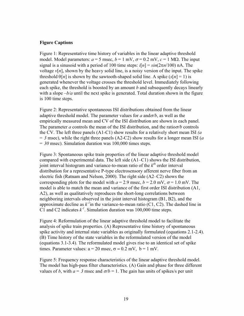
Figure Captions Figure 1: Representative time history of variables in the linear adaptive threshold model. Model parameters: a = 5 msec, b = 1 mV, σ = 0.2 mV, c = 1 MΩ. The input signal is a sinusoid with a period of 100 time steps: i[n] = sin(2πn/100) nA. The voltage v[n], shown by the heavy solid line, is a noisy version of the input. The spike threshold θ[n] is shown by the sawtooth-shaped solid line. A spike (s[n] = 1) is generated whenever the voltage crosses the threshold level. Immediately following each spike, the threshold is boosted by an amount b and subsequently decays linearly with a slope –b/a until the next spike is generated. Total duration shown in the figure is 100 time steps. Figure 2: Representative spontaneous ISI distributions obtained from the linear adaptive threshold model. The parameter values for a andσ/b, as well as the empirically measured mean and CV of the ISI distribution are shown in each panel. The parameter a controls the mean of the ISI distribution, and the ratioσ/b controls the CV. The left three panels (A1-C1) show results for a relatively short mean ISI (a = 3 msec), while the right three panels (A2-C2) show results for a longer mean ISI (a = 30 msec). Simulation duration was 100,000 times steps. Figure 3: Spontaneous spike train properties of the linear adaptive threshold model compared with experimental data. The left side (A1–C1) shows the ISI distribution, joint interval histogram and variance-to-mean ratio of the kth order interval distribution for a representative P-type electrosensory afferent nerve fiber from an electric fish (Ratnam and Nelson, 2000). The right side (A2–C2) shows the corresponding plots for the model with a = 2.9 msec, b = 2.0 mV, σ = 1.0 mV. The model is able to match the mean and variance of the first order ISI distribution (A1, A2), as well as qualitatively reproduces the short-long correlations between neighboring intervals observed in the joint interval histogram (B1, B2), and the approximate decline as k-1in the variance-to-mean ratio (C1, C2). The dashed line in C1 and C2 indicates k-1. Simulation duration was 100,000 time steps. Figure 4: Reformulation of the linear adaptive threshold model to facilitate the analysis of spike train properties. (A) Representative time history of spontaneous spike activity and internal state variables as originally formulated (equations 2.1-2.4). (B) Time history of the state variables in the reformulated version of the model (equations 3.1-3.4). The reformulated model gives rise to an identical set of spike times. Parameter values: a = 20 msec, σ = 0.2 mV, b = 1 mV. Figure 5: Frequency response characteristics of the linear adaptive threshold model. The model has high-pass filter characteristics. (A) Gain and phase for three different values of b, with a = 3 msec and σ/b = 1. The gain has units of spikes/s per unit

20

input. The gain varies inversely with b; the phase curves are overlapping and indistinguishable. (B) Gain and phase for three different values of a, with b = 0.1 mV and σ = 0.1 mV. The parameter a influences the corner frequency of the high-pass filter. Simulation duration was 100,000 time steps for a = 3 msec and a = 10 msec, and 500,000 time steps for a = 30 msec. Figure 6: Frequency response characteristics of the exponential adaptive threshold model compared with experimental data. The left panels show the spontaneous spike train properties of the model: (A) ISI distribution, and (B) variance-to-mean ratio of the kth order interval distribution. The right panel (C) shows gain and phase of the driven response. The data points show the population-averaged responses from 99 P-type electrosensory afferent fibers (modified from Nelson et al., 1997). Error bars represent the standard deviation of the population average at each frequency. The continuous solid lines show the gain and phase of the exponential adaptive threshold model with b = 0.11 mV, σ = 0.04 mV, θ0 = −1 mV, τf = 2 msec, and τθ = 30 msec. Simulation duration was 300,000 time steps. Figure 7: Comparison of two neural models with matched spontaneous ISI and driven response characteristics. The left side (A1-C1) shows results for the linear adaptive threshold model (equations 2.1-2.4), while the right side (A2-C2) shows an integrate-and-fire based model with a random threshold (equations 5.1-5.5). The model parameters were adjusted to yield similar first-order ISI distributions (A1, A2) and similar frequency response characteristics (B1, B2). However, the higher-order interval statistics, as characterized by the variance-to-mean ratio of kth order interval distribution, are quite different (C1, C2). The linear adaptive threshold model exhibits strong regularizing effects at large interval orders, whereas the random threshold model has variance-to-mean that is independent of interval order. Figure 8: Comparison of signal detectability for the linear adaptive threshold (A1-C1) and random threshold (A2-C2) models. The upper panels (A1, A2) show the stimulus waveform (arbitrary units), dot raster displays of representative spike activity, and post-stimulus rate histograms computed by averaging spike activity over 1000 stimulus trials. A solid white line shows a sinusoidal fit to the response. The middle panels (B1, B2) show histograms of the matched filter output for trials with and without a stimulus. The bottom panels (C1, C2) illustrate the dramatic improvement in detectability for signals encoded by the adaptive threshold model relative to the random threshold model, as measured by the ROC curves. The dashed lines indicate chance-level performance.

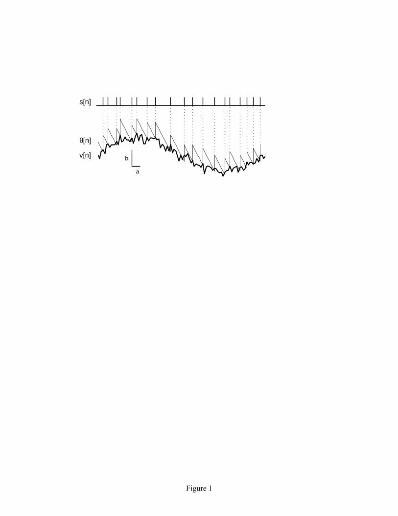
Figure 1

b

a

v[n]

θ[n]

s[n]

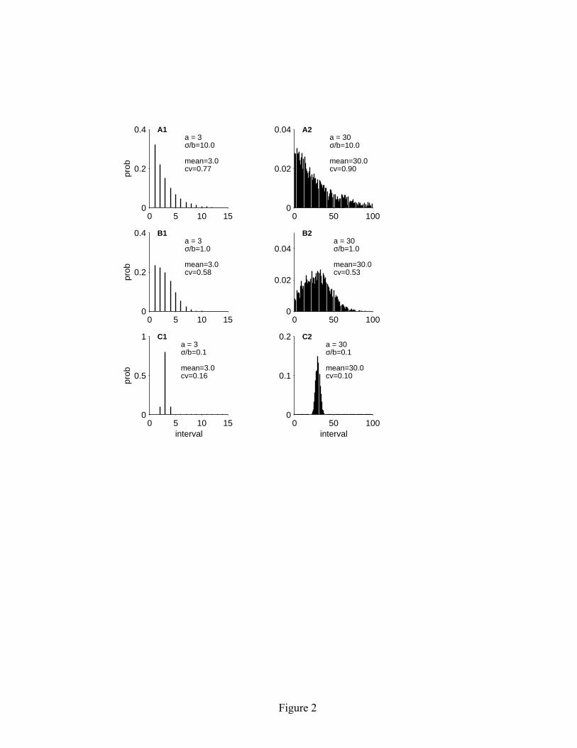
Figure 2

0 5 10 150

0.2

0.4pr

obA1

a = 3σ/b=10.0

mean=3.0cv=0.77

0 5 10 150

0.2

0.4

prob

B1a = 3σ/b=1.0

mean=3.0cv=0.58

0 5 10 150

0.5

1

interval

prob

C1a = 3σ/b=0.1

mean=3.0cv=0.16

0 50 1000

0.02

0.04 A2a = 30σ/b=10.0

mean=30.0cv=0.90

0 50 1000

0.02

0.04

B2a = 30σ/b=1.0

mean=30.0cv=0.53

0 50 1000

0.1

0.2

interval

C2a = 30σ/b=0.1

mean=30.0cv=0.10

Figure 3

0 5 100

0.1

0.2

0.3Model

interval

A2

mean=2.9

cv=0.46

0 2 4 60

2

4

6

interval j

B2

1 10 1000.01

0.1

1

order k

C2

0 5 100

0.1

0.2

0.3Data

interval

prob

A1

mean=2.9

cv=0.46

0 2 4 60

2

4

6

interval j

inte

rval

j+

1

B1

1 10 1000.01

0.1

1

order k

varia

nce/

mea

n

C1

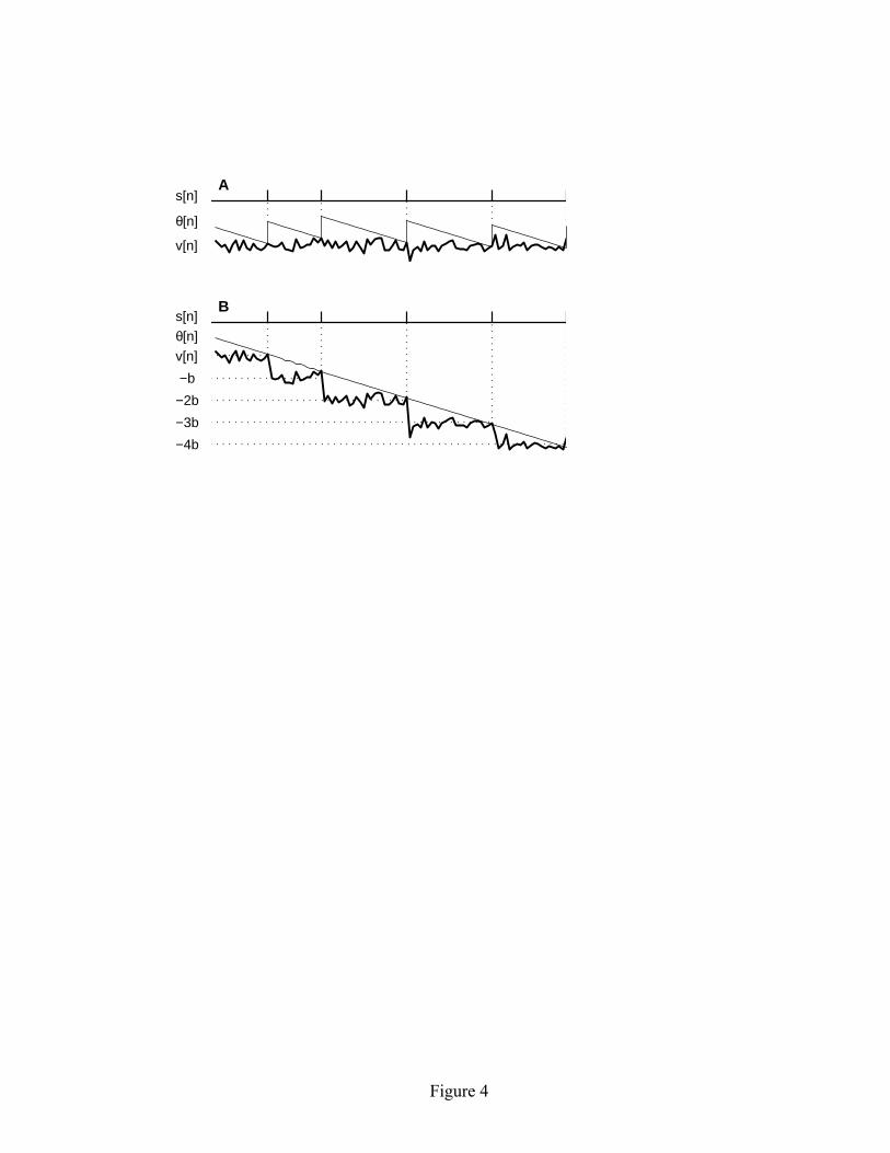
Figure 4

A

v[n]

θ[n]

s[n]

B

θ[n]

s[n]

v[n]

−b

−2b

−3b

−4b

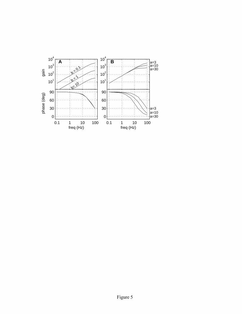
Figure 5

101

102

103

104

A

b = 0.1

b = 1

b= 10

gain

101

102

103

104

B a=3a=10a=30

0.1 1 10 100

0

30

60

90

freq (Hz)

phas

e (d

eg)

0.1 1 10 100

0

30

60

90

freq (Hz)

a=3a=10a=30

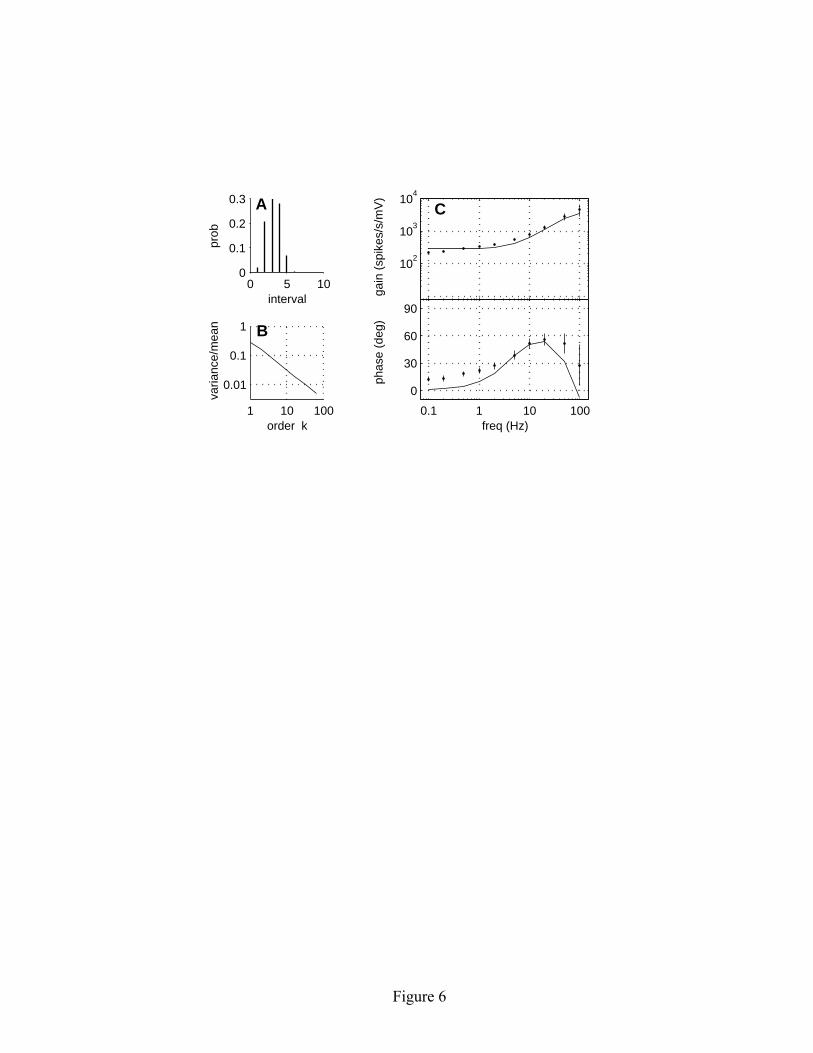
Figure 6

102

103

104

gain

(sp

ikes

/s/m

V)

C

0.1 1 10 100

0

30

60

90

freq (Hz)

phas

e (d

eg)

0 5 100

0.1

0.2

0.3

interval

prob

A

1 10 100

0.01

0.1

1

order k

varia

nce/

mea

n B

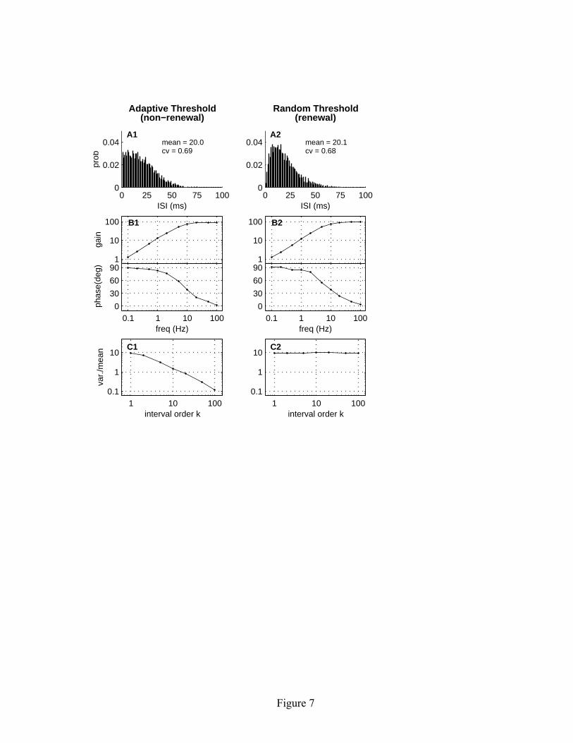
Figure 7

0 25 50 75 1000

0.02

0.04

ISI (ms)

prob

Adaptive Threshold(non−renewal)

A1mean = 20.0cv = 0.69

1

10

100

gain

B1

0.1 1 10 1000

30

60

90

freq (Hz)

phas

e(de

g)

1 10 1000.1

1

10

interval order k

var.

/mea

n C1

0 25 50 75 1000

0.02

0.04

ISI (ms)

Random Threshold(renewal)

A2mean = 20.1cv = 0.68

1

10

100 B2

0.1 1 10 1000

30

60

90

freq (Hz)

1 10 1000.1

1

10

interval order k

C2

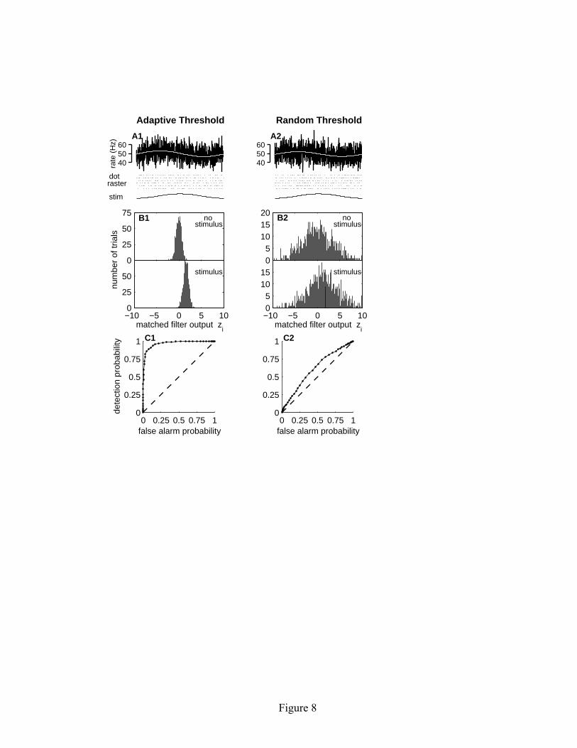
Figure 8

605040ra

te (

Hz)

dotraster

stim

A1

Adaptive Threshold

605040

A2

Random Threshold

0

25

50

75

num

ber

of tr

ials

B1 nostimulus

−10 −5 0 5 100

25

50

matched filter output zi

stimulus

05

101520 B2 no

stimulus

−10 −5 0 5 1005

1015

matched filter output zi

stimulus

0 0.25 0.5 0.75 10

0.25

0.5

0.75

1

false alarm probability

dete

ctio

n pr

obab

ility C1

0 0.25 0.5 0.75 10

0.25

0.5

0.75

1

false alarm probability

C2