COLLEGE OF AGRICULTURE AND LIFE SCIENCES

TR-363

2010

A Simple Model for Estimating Water Balance

and Salinity of Reservoirs and Outflow

By: S. Miyamoto, F. Yuan, and Shilpa Anand

Texas AgriLife Research and Extension Center at El Paso

Texas Water Resources Institute Technical Report No. 363 Texas A&M University System

College Station, Texas 77843-2118

June 2009

A SIMPLE MODEL FOR ESTIMATING WATER BALANCE AND SALINITY OF RESERVOIRS AND OUTFLOW

S. Miyamoto, F. Yuan, and Shilpa Anand

TWRI: TR 363 .

June 2009

Texas A&M University AgriLife Research Center at El Paso

Red Bluff

Amistad Elephant Butte

PREFACE

Many river basins of the western U.S. were initially developed for crop irrigation, mostly after the passage of the Reclamation Act of 1906. The diversion for irrigation reduced streamflow and increased salinity downstream. Reduced streamflow, especially reduced bank overflow, caused salinization of floodplains in the presence of a high water table. This was accompanied by the spread of salt-tolerant riparian species, especially saltcedar (Tamarisk sp.). This scenario is repeated in many river systems in the Southwest.

There are considerable interests in restoring degradated river systems. Saltcedar control is for example, widely implemented through chemical application or biological control methods. It is viewed as the first step towards restoring the riparian ecosystem. In addition, there has been an expectation that saltcedar control may result in increased flow and reduced salinity. However, this expectation has to be examined carefully. Controlled flooding through reservoir water release has also been attempted in an effort to maintain the original ecosystems. Increasing efforts are also being made to identify and control saline water intrusion in an attempt to lower salinity.

The models described in this series were developed mainly to help evaluate river management options on flow and salinity of the stream and the floodplains. The first part deals with water and salt balance in reservoirs. The primary purpose of the model is to predict outflow salinity from the reservoir storage and inflow information in advance of the actual release. A simple two-layer model is used to describe the reservoir processes. The second part addresses water and salt transport through semi-arid river channels. A routing model referred to as ROTO (developed at the Blackland Soil and Water Conservation Laboratory at Temple, Texas) was used to simulate streamflow and salinity on a daily time step. This model also provides the estimate of evaporation and percolation losses of water, the interaction between streamflow and shallow groundwater, and the bank overflow required for estimating salt leaching from the floodplains. Salt transport processes were added to the ROTO model so as to estimate the changes in streamflow salinity. The third part concerns with water and salt storage in the riparian zones. The models are coded in FORTRAN and are available upon request.

The models were applied to the middle reach of the Pecos River (Malaga, New Mexico, to Girvin, Texas) and, to a limited extent, to selected sites along the Rio Grande, and were found workable using mostly existing database.

ACKNOWLEDGEMENT

The information presented in this report was gathered primarily for an EPA project entitled “Basin-wide Management Plan for the Pecos River in Texas” under a contract No. 4280001. The cost of analyses and document preparation was defrayed in part by the Cooperative State Research, Education, and Extension Service, U.S. Department of Agriculture under Agreement No. 2001-45049-01149, and by the state fund for Agrilife Research of the Texas A & M University System. Document preparation was assisted by Nancy Hanks, Research Associate, and Vanessa Garcia and Elsa Bonilla, Student Workers at the Texas A&M University Agricultural Research Center at El Paso.

CONTENTS

ABSTRACT............................................................................................................................................... 1

INTRODUCTION..................................................................................................................................... 1

1. MODEL DESCRIPTION.................................................................................................................... 2

1.1 Water and Salt Loading Estimates.................................................................................. 2

1.2 Simulation of Reservoir Processes................................................................................... 4

1.3 Data Required ................................................................................................................... 4

1.4 Computational Procedures .............................................................................................. 5

2. MODEL APPLICATION ................................................................................................................... 7

2.1 Red Bluff Reservoir .......................................................................................................... 7

2.1.1 Data Used ............................................................................................................... 7

2.1.2 Data Processing ..................................................................................................... 9

2.1.3 Results .................................................................................................................. 11

2.2 Elephant Butte, Amistad, and Falcon ........................................................................... 17

2.2.1 Data Used and Computational Procedures ...................................................... 17

2.2.2 Results and Discussion........................................................................................ 19

REFERENCES........................................................................................................................................ 21

Unit Conversion

1 km = 3.3 ft 1 m3 = 35.3 ft3 1 m3/s = 22.8 mgp 1 km = 0.621 miles 1 Mm3 = 811 acre-ft 1 ha = 2.47 acres 1 m3/s = 35.3 cfs

1

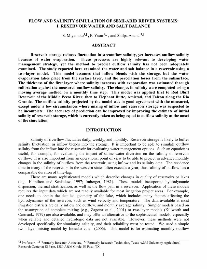
FLOW AND SALINITY SIMULATION OF SEMI-ARID REIVER SYSTEMS: I. RESERVOIR WATER AND SALT BALANCE

S. Miyamoto1┘, F. Yuan 2┘, and Shilpa Anand 3┘

ABSTRACT

Reservoir storage reduces fluctuation in streamflow salinity, yet increases outflow salinity

because of water evaporation. These processes are highly relevant to developing water management strategy, yet the method to predict outflow salinity has not been adequately examined. The study reported here examined the water and salt balance in a reservoir using a two-layer model. This model assumes that inflow blends with the storage, but the water evaporation takes place from the surface layer, and the percolation losses from the subsurface. The thickness of the first layer where salinity increases with evaporation was estimated through calibration against the measured outflow salinity. The changes in salinity were computed using a moving average method on a monthly time step. This model was applied first to Red Bluff Reservoir of the Middle Pecos River, then to Elephant Butte, Amistad, and Falcon along the Rio Grande. The outflow salinity projected by the model was in good agreement with the measured, except under a few circumstances where mixing of inflow and reservoir storage was suspected to be incomplete. The accuracy of prediction can be improved by improving the estimate of initial salinity of reservoir storage, which is currently taken as being equal to outflow salinity at the onset of the simulation.

INTRODUCTION

Salinity of riverflow fluctuates daily, weekly, and monthly. Reservoir storage is likely to buffer salinity fluctuation, as inflow blends into the storage. It is important to be able to simulate outflow salinity from the inflow into the reservoir for evaluating water management options. Such an equation is useful, for example, for evaluating the impact of saline water diversion on the salinity of reservoir outflow. It is also important from an operational point of view to be able to project in advance monthly changes in the salinity of outflow from the reservoir, using inflow and its salinity data. The residence time in many of the reservoirs in the western states often exceeds a year, thus salinity of outflow has a comparable duration of time-lag.

There are many sophisticated models which describe changes in quality of reservoirs or lakes (e.g., Hamilton and Schladow, 1997; Imberger, 1981). These models incorporate hydrodynamic dispersion, thermal stratification, as well as the flow path in a reservoir. Application of these models requires the input data which are not readily available for most irrigation project areas. For example, one needs to obtain the detailed geometry of the lake, which includes many factors affecting the hydrodynamics of the reservoir, such as wind velocity and temperature. The data available at most irrigation districts are daily inflow and outflow, and monthly average salinity. Simpler models based on the assumption of complete mixing (e.g., Zagona et al., 2001) or two-layer models (Killworth and Carmack, 1979) are also available, and may offer an alternative to the sophisticated models, especially when reliable and detailed hydrologic data are not available. However, these methods were notdeveloped specifically for simulating salinity, and their reliability must be tested. We used a simple two- layer mixing model by Inosako et al. (2006). This model is for estimating monthly outflow

1┘Professor, 2┘ Formerly Research Associate, 3┘Formerly Research Technician, Texas A&M University Agricultural Research Center at El Paso, 1380 A&M Circle, El Paso, TX.

2

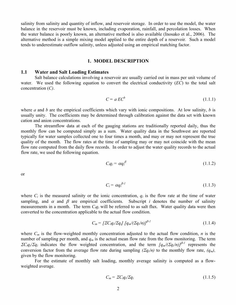
salinity from salinity and quantity of inflow, and reservoir storage. In order to use the model, the water balance in the reservoir must be known, including evaporation, rainfall, and percolation losses. When the water balance is poorly known, an alternative method is also available (Inosako et al., 2006). The alternative method is a simple mixing model applied to the entire depth of a reservoir. Such a model tends to underestimate outflow salinity, unless adjusted using an empirical matching factor.

1. MODEL DESCRIPTION 1.1 Water and Salt Loading Estimates

Salt balance calculations involving a reservoir are usually carried out in mass per unit volume of water. We used the following equation to convert the electrical conductivity (EC) to the total salt concentration (C).

C = a ECb (1.1.1)

where a and b are the empirical coefficients which vary with ionic compositions. At low salinity, b is usually unity. The coefficients may be determined through calibration against the data set with known cation and anion concentrations.

The streamflow data at each of the gauging stations are traditionally reported daily, thus the monthly flow can be computed simply as a sum. Water quality data in the Southwest are reported typically for water samples collected one to four times a month, and may or may not represent the true quality of the month. The flow rates at the time of sampling may or may not coincide with the mean flow rate computed from the daily flow records. In order to adjust the water quality records to the actual flow rate, we used the following equation.

Ciqi = αqiβ (1.1.2)

or

Ci = αqiβ-1 (1.1.3)

where Ci is the measured salinity or the ionic concentration, qi is the flow rate at the time of water sampling, and α and β are empirical coefficients. Subscript i denotes the number of salinity measurements in a month. The term Ciqi will be referred to as salt flux. Water quality data were then converted to the concentration applicable to the actual flow condition.

Cm = [ΣCiqi/Σqi] [qm/(Σqi/n)]β-1 (1.1.4)

where Cm is the flow-weighted monthly concentration adjusted to the actual flow condition, n is the number of sampling per month, and qm is the actual mean flow rate from the flow monitoring. The term ΣCiqi/Σqi indicates the flow weighted concentration, and the term [qm/(Σqi/n)]β-1 represents the conversion factor from the average flow rate during sampling (Σqi/n) to the monthly flow rate, (qm), given by the flow monitoring.

For the estimate of monthly salt loading, monthly average salinity is computed as a flow-weighted average.

Cm = ΣCiqi/Σqi (1.1.5)

3

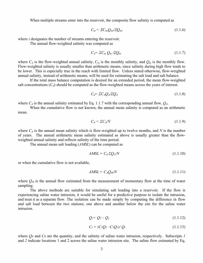
When multiple streams enter into the reservoir, the composite flow salinity is computed as

Cm = ΣCmiQmi/ΣQmi (1.1.6)

where i designates the number of streams entering the reservoir. The annual flow-weighted salinity was computed as

CA= ΣCm Qm /ΣQm (1.1.7)

where CA is the flow-weighted annual salinity, Cm is the monthly salinity, and Qm is the monthly flow. Flow-weighted salinity is usually smaller than arithmetic means, since salinity during high flow tends to be lower. This is especially true in the reach with limited flow. Unless stated otherwise, flow-weighted annual salinity, instead of arithmetic means, will be used for estimating the salt load and salt balance.

If the total mass balance computation is desired for an extended period, the mean flow-weighted salt concentrations (Cd) should be computed as the flow-weighted means across the years of interest.

Cd= ΣCAQA/ΣQA (1.1.8)

where CA is the annual salinity estimated by Eq. 1.1.7 with the corresponding annual flow, QA. When the cumulative flow is not known, the annual mean salinity is computed as an arithmetic

mean.

CA = ΣCA/N (1.1.9) where CA is the annual mean salinity which is flow-weighted up to twelve months, and N is the number of years. The annual arithmetic mean salinity estimated as above is usually greater than the flow-weighted annual salinity and reflects salinity of the time period.

The annual mean salt loading (AMSL) can be computed as

AMSL = Cd ΣQA/N (1.1.10)

or when the cumulative flow is not available,

AMSL = CAQM/N (1.1.11) where QM is the annual flow estimated from the measurement of momentary flow at the time of water sampling.

The above methods are suitable for simulating salt loading into a reservoir. If the flow is experiencing saline water intrusion, it would be useful for a predictive purpose to isolate the intrusion, and treat it as a separate flow. The isolation can be made simply by computing the difference in flow and salt load between the two stations; one above and another below the site for the saline water intrusion.

Qs = Q2 – Q1 (1.1.12)

Cs = (C2Q2 –C1Q1)/ Qs (1.1.13) where Qs and Cs are the quantity, and the salinity of saline water intrusion, respectively. Subscripts 1 and 2 indicate locations 1 and 2 across the saline water intrusion site. The saline flow estimated by Eq.

4

1.1.12 and 1.1.13 can be treated as a separate flow when computing the mean inflow by Eq. 1.1.6. When Qs is very small, Eq. 1.1.13 can become infinity. In that case, saline water intrusion

should be treated as

CsQs = C2Q2 – C1Q1 (1.1.14)

where CsQs will be referred to as the intrusion flux. 1.2 Simulation of Reservoir Processes

The reservoir processes include mixing, evaporation, and percolation losses. The methods proposed by Inosako et al. (2006) allow several ways to compute the water balance. We used the following monthly water balance.

Sj = Sj-1 + (QINj – QOUTj) – (Ej – Rj) – Pj (1.2.1)

where Sj is the reservoir storage of the j month (m3), QIN the monthly inflow, QOUT the monthly outflow, E the evaporation, R the rainfall, and P the percolation loss.

The evaporation from the free water surface can be computed from the pan evaporation (Epan) or the potential evaporation estimated from climatic data.

E = AKpEpan (1.2.2) where E is the evaporative water losses from the water surface A (m2), Kp the pan coefficient, and Epan the pan evaporation.

We used a two-layer model to estimate salinity of the outflow. The top layer was assumed to be subject to evaporation and rainfall, the second layer the percolation losses.

Cj-1Sj-1 + CINjQINj – Cj-1Pj (1.2.3) Sj-1 + QINj – Pj

COUTj = dAjCj / (dAj – Ej + Rj) (1.2.4)

where COUTj is the outflow salinity, d is the depth of the reservoir subject to evaporative concentration, A the water surface area, and E, R, and P are defined earlier in Eq. 1.2.1. The evaporation minus rainfall (E – R) was assumed to affect the top layer of a thickness of d. The resulting storage Sj is then estimated by Eq. 1.2.1, incorporating the evaporation, the percolation loss and the outflow. The thickness of the top layer is to be estimated through calibration using Eq. 1.2.4. 1.3 Data Required

Two sets of data are required to estimate the reservoir water and salt balance. The first set specifies the water and salt loading into the reservoir, and includes salinity (C) and the conductivity (EC) relationship given by Eq. 1.1.1, salinity (C), and flow (q) relationship given by Eq. 1.1.2 and Eq. 1.1.4. The second set specifies reservoir processes, and includes inflow (QIN), outflow (QOUT), evaporation (E), rainfall (R), and reservoir storage (S). The water evaporation is estimated by using the pan evaporation data (Epan) with a known pan coefficient (Kp), and the estimates water surface area (A). The percolation losses (P) are estimates by rewriting Eq. 1.2.1 for P. Additional input data are given in Section 1.4.

Cj =

5

1.4 Computational Procedures

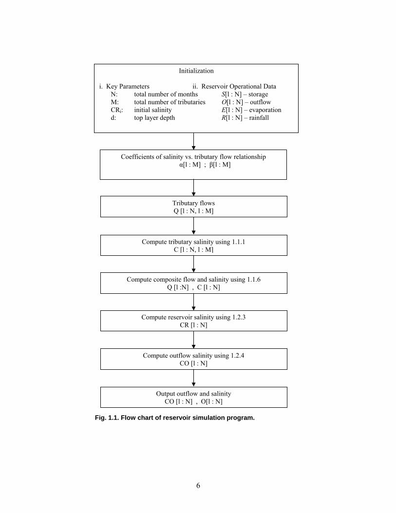
RSP (Reservoir Simulation Program) is a stand-alone program to simulate reservoir salinity based on the algorithm described. The source code for the reservoir simulation program is available as a FORTRAN 95 file (RSP.F95). This file is compiled and linked to create an executable file (RSP.EXE), using Lahey Fortran Compiler (LF95 v7.1). The program runs in a MS-DOS interface. To run this program type in RSP in MS-DOS mode, then the instructions to the program operation will appear. Input files: There are three needed input files, PARA.CSV, INFLOW.CSV, and RESERVOIR.CSV. The input files PARA.CSV defines the total number of months to simulate (N), and the total number of tributaries (M) that fill the reservoir (Fig. 1.1). In this program, users are required to input α and β, the two coefficients used in Eq. 1.1.2 to estimate monthly salinity of various inflows into the reservoir. INFLOW.CSV defines the monthly flow rate of various tributaries. Note that units are in million cubic meters per month (Mm3/mo). RESERVOIR.CSV defines the months of reservoir simulation, expressed as decimal percentage of a year (YR), reservoir storage (S, Mm3), outflow volume (O, Mm3/mo), evaporate rate (E, cm/mo) and precipitation (R, cm/mo). Note that units for evaporation rate and precipitation rate are in cm because their absolute volumes are related to the water surface area (A) which is computed in the program, using a calibration equation applicable to a given reservoir. The evaporative loss is then converted to a volume unit in the program. Computation: Once input sequences are completed, the program is directed to compute salinity of tributaries by Eq. 1.1.3, and salinity of the composite inflow by Eq. 1.1.6. It will then proceed to compute reservoir salinity by Eq. 1.2.3. Salinity of the initial reservoir storage was assumed to be equal to salinity of the outflow. This could be improved by using salinity of the composite flow adjusted to water evaporation. Salinity of subsequent months was then computed as a moving average. The estimated salinity of the outflow by Eq. 1.2.4 was compared against the measured to calibrate the depth of the top layer subjected to water evaporation during the calibration run.

Output Files: The simulated results are stored in a file called OUT.DAT, which includes volume of composite inflow (Q, Mm3/mo), salinity of composite inflow (C, mg/L), evaporation (E, Mm3/mo), rainfall (R, Mm3/mo), percolation (P, Mm3/mo), reservoir storage (S, Mm3), outflow volume (O, Mm3/mo), reservoir salinity (CR, mg/L), and outflow salinity (CO, mg/L) on a monthly time step.

1.5 Nomenclature C the total salt concentration (mg/l) EC the electrical conductivity (dS m-1) Ci the measured salinity of a tributary (mg/l) qi the measured flow rate at the time of water

sampling (m3/s) Cm the flow-weighted monthly salinity

adjusted to the actual flow rate (mg/l) CA the flow-weighted annual salinity (mg/l) Cd the flow-weighted multi-year salinity

(mg/l) CS the salinity of intruding water (mg/l) Sj the reservoir storage at month j (Mm3) QINj the monthly inflow at month j (Mm3)

QOUTj the monthly outflow at month j (Mm3) QS the monthly flow of intruding water

(Mm3) Ej the monthly evaporation at month j (Mm3) Rj the monthly rainfall at month j (cm/mo) Pj the monthly percolation loss of month j

(Mm3) Kp the pan coefficient (~ 0.7) Epan the pan evaporation rate (cm/mo) A the surface area of the reservoir (m2)

AMSL the annual mean salt loading (tons/yr)

d the depth of the reservoir subject to evaporative concentration (m)

6

Output outflow and salinity CO [l : N] , O[l : N]

Compute outflow salinity using 1.2.4 CO [l : N]

Compute reservoir salinity using 1.2.3 CR [l : N]

Initialization

i. Key Parameters ii. Reservoir Operational Data N: total number of months S[l : N] – storage M: total number of tributaries O[l : N] – outflow CRi: initial salinity E[l : N] – evaporation d: top layer depth R[l : N] – rainfall

Coefficients of salinity vs. tributary flow relationship α[l : M] ; β[l : M]

Tributary flows Q [l : N, l : M]

Compute tributary salinity using 1.1.1 C [l : N, l : M]

Compute composite flow and salinity using 1.1.6 Q [l :N] , C [l : N]

Fig. 1.1. Flow chart of reservoir simulation program.

7

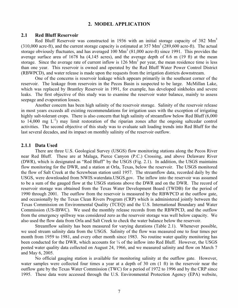
2. MODEL APPLICATION 2.1 Red Bluff Reservoir

Red Bluff Reservoir was constructed in 1936 with an initial storage capacity of 382 Mm3 (310,000 acre-ft), and the current storage capacity is estimated at 357 Mm3 (289,600 acre-ft). The actual storage obviously fluctuates, and has averaged 100 Mm3 (81,000 acre-ft) since 1991. This provides the average surface area of 1678 ha (4,145 acres), and the average depth of 6.6 m (19 ft) at the mean storage. Since the average rate of current inflow is 126 Mm3 per year, the mean residence time is less than one year. This reservoir is owned and operated by the Red Bluff Water Power Control District (RBWPCD), and water release is made upon the requests from the irrigation districts downstream.

One of the concerns is reservoir leakage which appears primarily in the southeast corner of the reservoir. The leakage from reservoirs in the Pecos Basin is suspected to be large. McMillan Lake, which was replaced by Brantley Reservoir in 1991, for example, has developed sinkholes and severe leaks. The first objective of this study was to examine the reservoir water balance, mainly to assess seepage and evaporation losses.

Another concern has been high salinity of the reservoir storage. Salinity of the reservoir release in most years exceeds all existing recommendations for irrigation uses with the exception of irrigating highly salt-tolerant crops. There is also concern that high salinity of streamflow below Red Bluff (6,000 to 14,000 mg L-1) may limit restoration of the riparian zones after the ongoing saltcedar control activities. The second objective of this study was to evaluate salt loading trends into Red Bluff for the last several decades, and its impact on monthly salinity of the reservoir outflow.

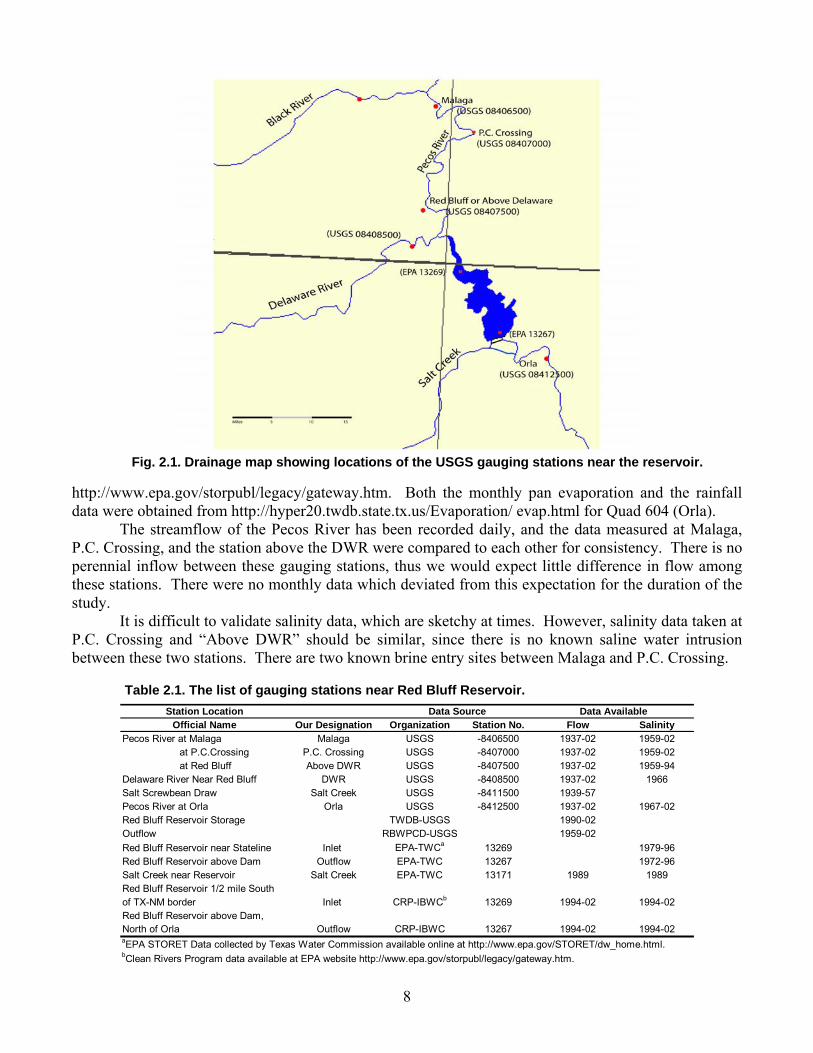
2.1.1 Data Used There are three U.S. Geological Survey (USGS) flow monitoring stations along the Pecos River near Red Bluff. These are at Malaga, Pierce Canyon (P.C.) Crossing, and above Delaware River (DWR), which is designated as “Red Bluff” by the USGS (Fig. 2.1). In addition, the USGS maintains flow monitoring for the DWR, and a station at Orla, Texas, below the reservoir. The USGS monitored the flow of Salt Creek at the Screwbean station until 1957. The streamflow data, recorded daily by the USGS, were downloaded from NWIS.waterdata.USGS.gov. The inflow into the reservoir was assumed to be a sum of the gauged flow at the USGS stations above the DWR and on the DWR. The record of reservoir storage was obtained from the Texas Water Development Board (TWDB) for the period of 1990 through 2001. The outflow from the reservoir is measured by the RBWPCD at the outflow gate, and occasionally by the Texas Clean Rivers Program (CRP) which is administered jointly between the Texas Commission on Environmental Quality (TCEQ) and the U.S. International Boundary and Water Commission (US-IBWC). We used the monthly release records from the RBWPCD, and the outflow from the emergency spillway was considered zero as the reservoir storage was well below capacity. We also used the flow data from Orla and Salt Creek to check the water balance below the reservoir.

Streamflow salinity has been measured for varying durations (Table 2.1). Whenever possible, we used stream salinity data from the USGS. Salinity of the flow was measured one to four times per month from 1959 to 1981, and every other month since 1983. No routine water quality monitoring has been conducted for the DWR, which accounts for ¼ of the inflow into Red Bluff. However, the USGS posted water quality data collected on August 24, 1966, and we measured salinity and flow on March 7 and May 6, 2005.

No official gauging station is available for monitoring salinity at the outflow gate. However, water samples were collected four times a year at a depth of 30 cm (1 ft) in the reservoir near the outflow gate by the Texas Water Commission (TWC) for a period of 1972 to 1996 and by the CRP since 1995. These data were accessed through the U.S. Environmental Protection Agency (EPA) website,

8

http://www.epa.gov/storpubl/legacy/gateway.htm. Both the monthly pan evaporation and the rainfall data were obtained from http://hyper20.twdb.state.tx.us/Evaporation/ evap.html for Quad 604 (Orla).

The streamflow of the Pecos River has been recorded daily, and the data measured at Malaga, P.C. Crossing, and the station above the DWR were compared to each other for consistency. There is no perennial inflow between these gauging stations, thus we would expect little difference in flow among these stations. There were no monthly data which deviated from this expectation for the duration of the study.

It is difficult to validate salinity data, which are sketchy at times. However, salinity data taken at P.C. Crossing and “Above DWR” should be similar, since there is no known saline water intrusion between these two stations. There are two known brine entry sites between Malaga and P.C. Crossing.

Fig. 2.1. Drainage map showing locations of the USGS gauging stations near the reservoir.

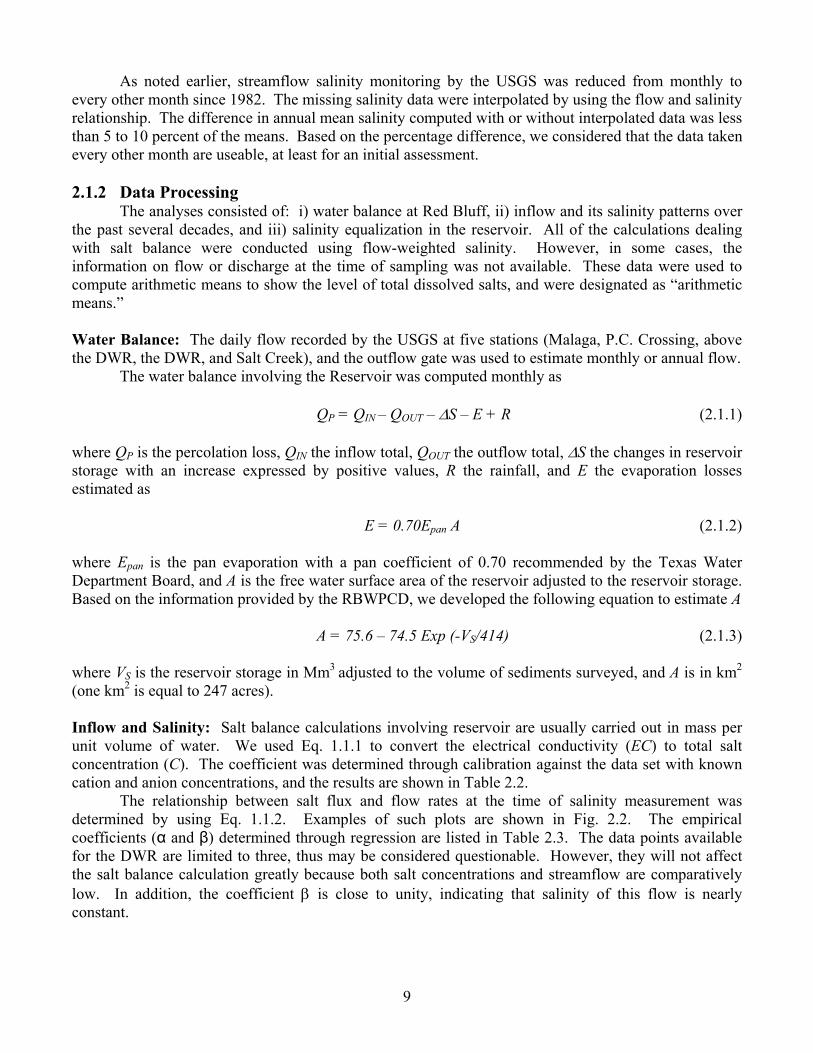
Station LocationOfficial Name Our Designation Organization Station No. Flow Salinity

Pecos River at Malaga Malaga USGS -8406500 1937-02 1959-02 at P.C.Crossing P.C. Crossing USGS -8407000 1937-02 1959-02 at Red Bluff Above DWR USGS -8407500 1937-02 1959-94Delaware River Near Red Bluff DWR USGS -8408500 1937-02 1966Salt Screwbean Draw Salt Creek USGS -8411500 1939-57Pecos River at Orla Orla USGS -8412500 1937-02 1967-02Red Bluff Reservoir Storage TWDB-USGS 1990-02Outflow RBWPCD-USGS 1959-02Red Bluff Reservoir near Stateline Inlet EPA-TWCa 13269 1979-96Red Bluff Reservoir above Dam Outflow EPA-TWC 13267 1972-96Salt Creek near Reservoir Salt Creek EPA-TWC 13171 1989 1989Red Bluff Reservoir 1/2 mile South of TX-NM borderRed Bluff Reservoir above Dam, North of Orla Outflow CRP-IBWC 13267 1994-02 1994-02aEPA STORET Data collected by Texas Water Commission available online at http://www.epa.gov/STORET/dw_home.html.bClean Rivers Program data available at EPA website http://www.epa.gov/storpubl/legacy/gateway.htm.

Data Source Data Available

Inlet CRP-IBWCb 13269 1994-02 1994-02

Table 2.1. The list of gauging stations near Red Bluff Reservoir.

9

As noted earlier, streamflow salinity monitoring by the USGS was reduced from monthly to every other month since 1982. The missing salinity data were interpolated by using the flow and salinity relationship. The difference in annual mean salinity computed with or without interpolated data was less than 5 to 10 percent of the means. Based on the percentage difference, we considered that the data taken every other month are useable, at least for an initial assessment. 2.1.2 Data Processing

The analyses consisted of: i) water balance at Red Bluff, ii) inflow and its salinity patterns over the past several decades, and iii) salinity equalization in the reservoir. All of the calculations dealing with salt balance were conducted using flow-weighted salinity. However, in some cases, the information on flow or discharge at the time of sampling was not available. These data were used to compute arithmetic means to show the level of total dissolved salts, and were designated as “arithmetic means.”

Water Balance: The daily flow recorded by the USGS at five stations (Malaga, P.C. Crossing, above the DWR, the DWR, and Salt Creek), and the outflow gate was used to estimate monthly or annual flow.

The water balance involving the Reservoir was computed monthly as

QP = QIN – QOUT – ΔS – E + R (2.1.1)

where QP is the percolation loss, QIN the inflow total, QOUT the outflow total, ΔS the changes in reservoir storage with an increase expressed by positive values, R the rainfall, and E the evaporation losses estimated as

E = 0.70Epan A (2.1.2)

where Epan is the pan evaporation with a pan coefficient of 0.70 recommended by the Texas Water Department Board, and A is the free water surface area of the reservoir adjusted to the reservoir storage. Based on the information provided by the RBWPCD, we developed the following equation to estimate A

A = 75.6 – 74.5 Exp (-VS/414) (2.1.3)

where VS is the reservoir storage in Mm3 adjusted to the volume of sediments surveyed, and A is in km2 (one km2 is equal to 247 acres). Inflow and Salinity: Salt balance calculations involving reservoir are usually carried out in mass per unit volume of water. We used Eq. 1.1.1 to convert the electrical conductivity (EC) to total salt concentration (C). The coefficient was determined through calibration against the data set with known cation and anion concentrations, and the results are shown in Table 2.2.

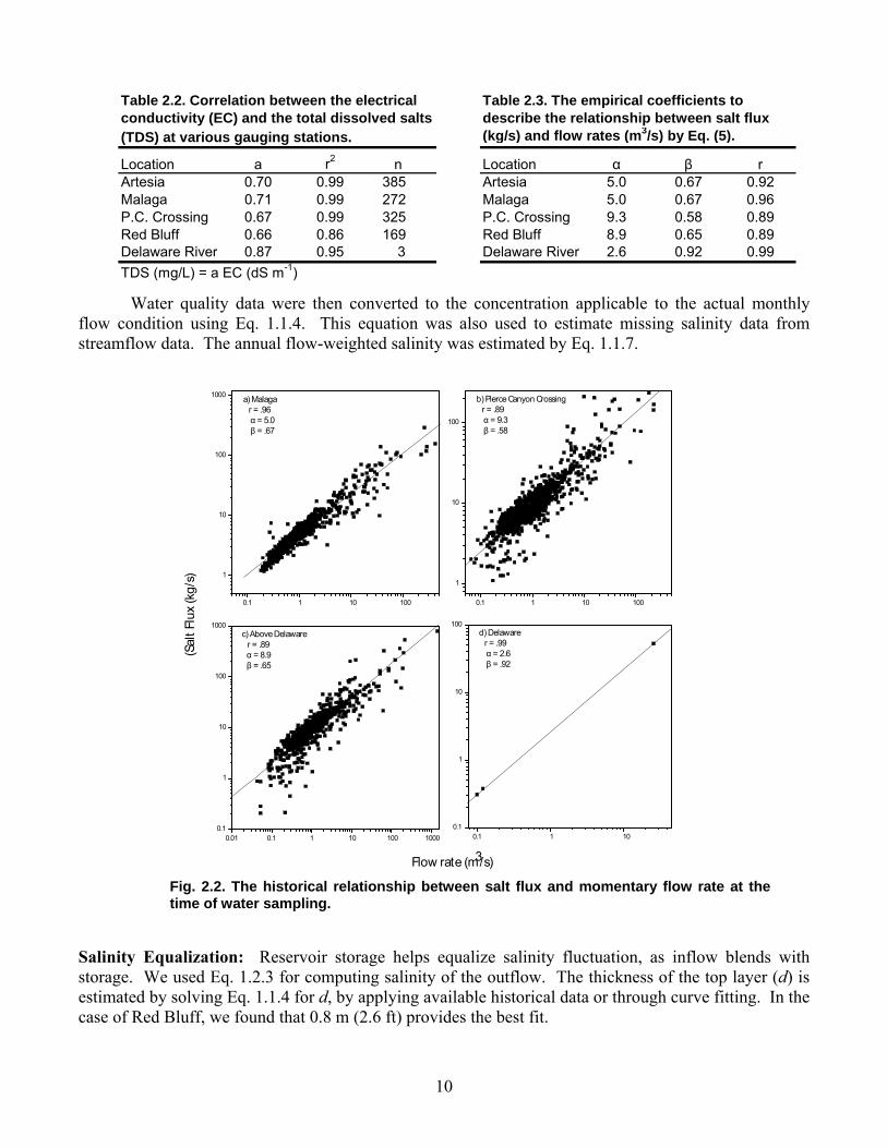
The relationship between salt flux and flow rates at the time of salinity measurement was determined by using Eq. 1.1.2. Examples of such plots are shown in Fig. 2.2. The empirical coefficients (α and β) determined through regression are listed in Table 2.3. The data points available for the DWR are limited to three, thus may be considered questionable. However, they will not affect the salt balance calculation greatly because both salt concentrations and streamflow are comparatively low. In addition, the coefficient β is close to unity, indicating that salinity of this flow is nearly constant.

10

Water quality data were then converted to the concentration applicable to the actual monthly flow condition using Eq. 1.1.4. This equation was also used to estimate missing salinity data from streamflow data. The annual flow-weighted salinity was estimated by Eq. 1.1.7.

Salinity Equalization: Reservoir storage helps equalize salinity fluctuation, as inflow blends with storage. We used Eq. 1.2.3 for computing salinity of the outflow. The thickness of the top layer (d) is estimated by solving Eq. 1.1.4 for d, by applying available historical data or through curve fitting. In the case of Red Bluff, we found that 0.8 m (2.6 ft) provides the best fit.

(kg/s) and flow rates (m3/s) by Eq. (5).

Location a r2 n Location α β rArtesia 0.70 0.99 385 Artesia 5.0 0.67 0.92Malaga 0.71 0.99 272 Malaga 5.0 0.67 0.96P.C. Crossing 0.67 0.99 325 P.C. Crossing 9.3 0.58 0.89Red Bluff 0.66 0.86 169 Red Bluff 8.9 0.65 0.89Delaware River 0.87 0.95 Delaware River 2.6 0.92 0.99TDS (mg/L) = a EC (dS m-1)

Table 2.3. The empirical coefficients to describe the relationship between salt flux

Table 2.2. Correlation between the electricalconductivity (EC) and the total dissolved salts (TDS) at various gauging stations.

3

0.01 0.1 1 10 100 10000.1

1

10

100

1000

0.1 1 10 100

1

10

100

0.1 1 100.1

1

10

100

0.1 1 10 100

1

10

100

1000

c) AboveDelawarer = .89α = 8.9β = .65

b) Pierce Canyon Crossingr = .89α = 9.3β = .58

Flow rate (m3/s)

d) Delawarer = .99α = 2.6β = .92

(Sal

t Flu

x (k

g/s)

a) Malagar = .96α = 5.0β = .67

Fig. 2.2. The historical relationship between salt flux and momentary flow rate at the time of water sampling.

11

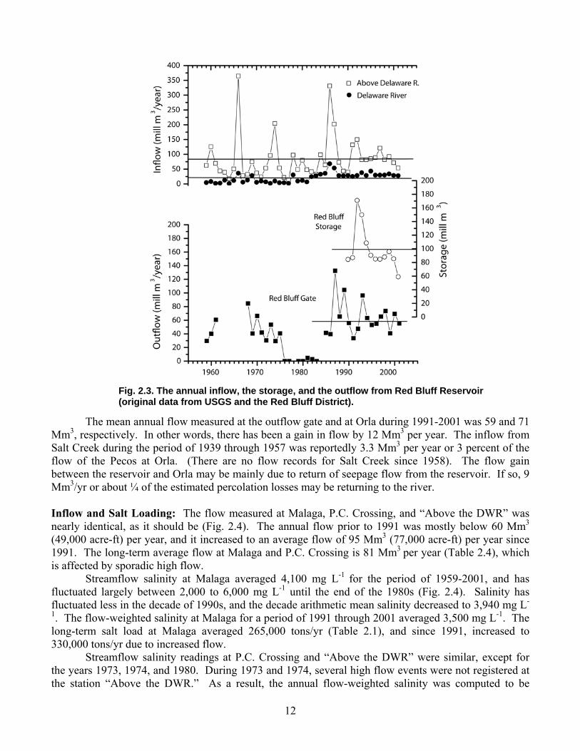
2.1.3 Results Water Balance: The flow of the Pecos measured at the station above the Delaware River (DWR) fluctuated widely with three large flow events during 1966 through 1986 (Fig. 2.3). These high flow events raised the mean annual flow to 84 Mm3 (68,000 acre-ft). If these three high flow events were omitted, the annual flow averaged 60 Mm3. The flow of the Pecos became relatively stable after 1991 (Fig. 2.3), and increased to 95 Mm3 per year for the last decade (Table 2.4). We suspect that the construction of the Brantley Dam in 1991 had a significant impact on flow control capability.

The flow of the DWR averaged 21 Mm3 (17,000 acre-ft) per year, which is 25 percent of the flow of the Pecos River. Since 1991, however, the flow has increased to 31 Mm3 per year for a reason unknown. The reservoir storage data prior to 1991 were not available. The mean storage since 1991 averaged 100 Mm3 (Table 2.4), less than 1/3 of the storage capacity of the Red Bluff Dam.

The inflow into the Red Bluff (sum of the flow of the Pecos and the DWR) during the period of 1991 through 2001 averaged 126 Mm3 (102,000 acre-ft) per year (Table 2.4). The outflow during the period was reported by the RBWPCD to be 59 Mm3 (49,000 acre-ft) per year. The reservoir storage change per year amounted to a reduction of 3.4 Mm3 per year for 1991-2001. The inflow minus the outflow averaged 67 Mm3 per year. After adjusting for the storage change and rainfall, it appears that half of the water flowed into the reservoir, 75 Mm3 (61,000 acre-ft), was lost, presumably for evaporation and percolation.

The mean water surface area since 1991 was 17 km2 (4,200 acres). The evaporation losses estimated using a pan coefficient of 0.70 are shown in Table 2.4, and the pan evaporation averaged 294 cm (114 inches) per year during the period of 1991 through 2001. The estimate of water evaporation from the reservoir was corrected for the surface area, and averaged 35 Mm3 (28,000 acre-ft) per year.

The percolation losses averaged 41 Mm3 (33,000 acre-ft) per year or 32 percent of the inflow. The percolation loss reached 60 Mm3 when the reservoir storage was large (186 Mm3). If the high percolation loss estimate for 1992 and 1995 is ignored, the percolation losses averaged 37 Mm3 (30,000 acre-ft), instead of 41 Mm3 shown in Table 2.4.

Table 2.4. The annual inflow, annual outflow, reservoir storage, surface area, rainfallevaporation, and percolation losses.

Outflow Surf Area Rainfall EVAP EVAP Percol Loss

YearAboveDWR DWR

RedBluff

RedBluff

RedBluff

RedBluff

RedBluff

RedBluff

Mm3 /y km2 Mm3 cm/y Mm3 Mm3

1990 (40)1- 29 56 _2- 843- 15 3.7 130 19 -1991 132 25 34 87 147 15 6.8 210 32 361992 150 29 47 171 186 26 13.5 170 45 611993 82 37 96 150 124 24 10.4 226 54 421994 82 29 63 109 100 18 4.4 236 43 321995 85 43 53 90 90 16 3.8 205 32 581996 89 30 55 85 91 15 7 218 32 371997 121 30 65 85 114 15 4 195 29 371998 82 30 73 88 85 15 4.7 230 35 381999 93 34 41 96 107 16 3.2 191 31 352000 72 29 69 85 80 15 3.4 196 29 322001 54 28 55 59 47 11 1.6 161 18 44Avg. 95 31 59 100 - 17 5.7 204 35 41

1-Incomplete data.2-Average storage for 1991 - 2001.3-End of year storage.

Mm3/y

Inflow

Mm3

StorageRedBluff

12

The mean annual flow measured at the outflow gate and at Orla during 1991-2001 was 59 and 71 Mm3, respectively. In other words, there has been a gain in flow by 12 Mm3 per year. The inflow from Salt Creek during the period of 1939 through 1957 was reportedly 3.3 Mm3 per year or 3 percent of the flow of the Pecos at Orla. (There are no flow records for Salt Creek since 1958). The flow gain between the reservoir and Orla may be mainly due to return of seepage flow from the reservoir. If so, 9 Mm3/yr or about ¼ of the estimated percolation losses may be returning to the river.

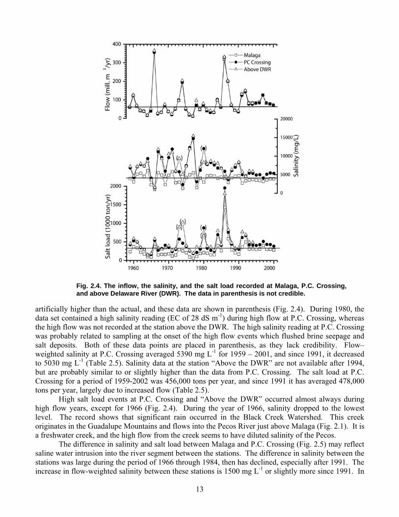
Inflow and Salt Loading: The flow measured at Malaga, P.C. Crossing, and “Above the DWR” was nearly identical, as it should be (Fig. 2.4). The annual flow prior to 1991 was mostly below 60 Mm3 (49,000 acre-ft) per year, and it increased to an average flow of 95 Mm3 (77,000 acre-ft) per year since 1991. The long-term average flow at Malaga and P.C. Crossing is 81 Mm3 per year (Table 2.4), which is affected by sporadic high flow.

Streamflow salinity at Malaga averaged 4,100 mg L-1 for the period of 1959-2001, and has fluctuated largely between 2,000 to 6,000 mg L-1 until the end of the 1980s (Fig. 2.4). Salinity has fluctuated less in the decade of 1990s, and the decade arithmetic mean salinity decreased to 3,940 mg L-

1. The flow-weighted salinity at Malaga for a period of 1991 through 2001 averaged 3,500 mg L-1. The long-term salt load at Malaga averaged 265,000 tons/yr (Table 2.1), and since 1991, increased to 330,000 tons/yr due to increased flow.

Streamflow salinity readings at P.C. Crossing and “Above the DWR” were similar, except for the years 1973, 1974, and 1980. During 1973 and 1974, several high flow events were not registered at the station “Above the DWR.” As a result, the annual flow-weighted salinity was computed to be

Fig. 2.3. The annual inflow, the storage, and the outflow from Red Bluff Reservoir (original data from USGS and the Red Bluff District).

13

artificially higher than the actual, and these data are shown in parenthesis (Fig. 2.4). During 1980, the data set contained a high salinity reading (EC of 28 dS m-1) during high flow at P.C. Crossing, whereas the high flow was not recorded at the station above the DWR. The high salinity reading at P.C. Crossing was probably related to sampling at the onset of the high flow events which flushed brine seepage and salt deposits. Both of these data points are placed in parenthesis, as they lack credibility. Flow–weighted salinity at P.C. Crossing averaged 5390 mg L-1 for 1959 – 2001, and since 1991, it decreased to 5030 mg L-1 (Table 2.5). Salinity data at the station “Above the DWR” are not available after 1994, but are probably similar to or slightly higher than the data from P.C. Crossing. The salt load at P.C. Crossing for a period of 1959-2002 was 456,000 tons per year, and since 1991 it has averaged 478,000 tons per year, largely due to increased flow (Table 2.5).

High salt load events at P.C. Crossing and “Above the DWR” occurred almost always during high flow years, except for 1966 (Fig. 2.4). During the year of 1966, salinity dropped to the lowest level. The record shows that significant rain occurred in the Black Creek Watershed. This creek originates in the Guadalupe Mountains and flows into the Pecos River just above Malaga (Fig. 2.1). It is a freshwater creek, and the high flow from the creek seems to have diluted salinity of the Pecos.

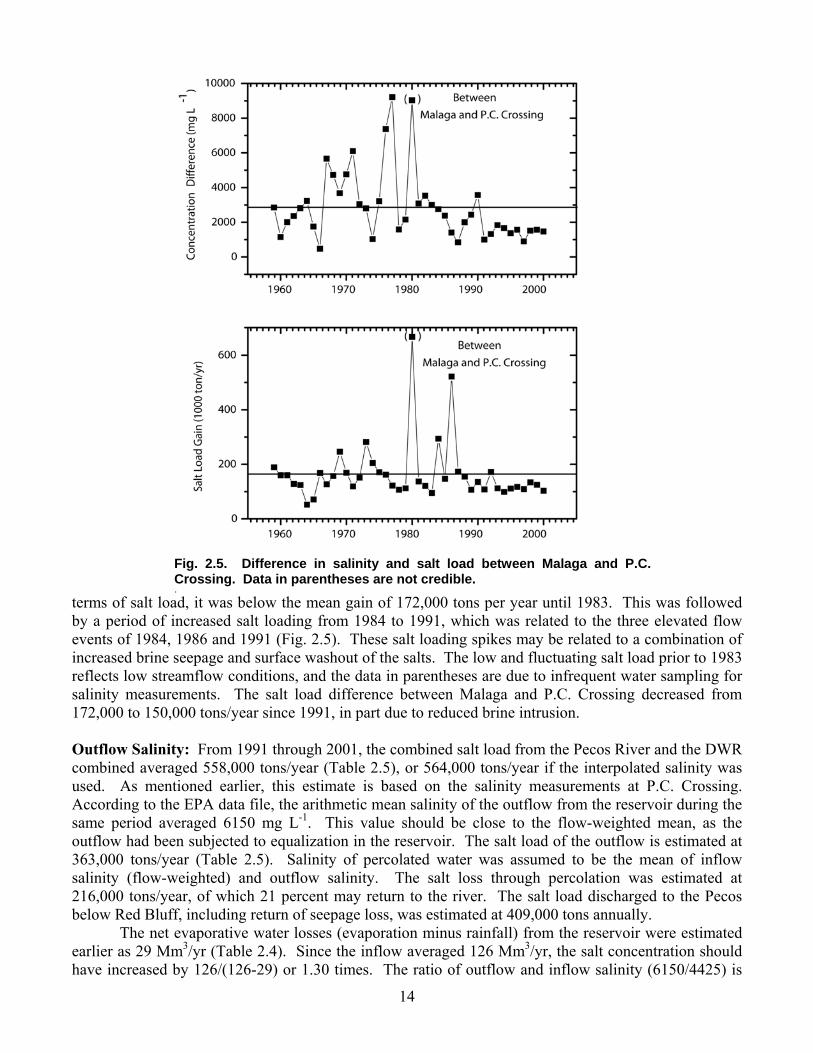
The difference in salinity and salt load between Malaga and P.C. Crossing (Fig. 2.5) may reflect saline water intrusion into the river segment between the stations. The difference in salinity between the stations was large during the period of 1966 through 1984, then has declined, especially after 1991. The increase in flow-weighted salinity between these stations is 1500 mg L-1 or slightly more since 1991. In

Fig. 2.4. The inflow, the salinity, and the salt load recorded at Malaga, P.C. Crossing,and above Delaware River (DWR). The data in parenthesis is not credible.

14

terms of salt load, it was below the mean gain of 172,000 tons per year until 1983. This was followed by a period of increased salt loading from 1984 to 1991, which was related to the three elevated flow events of 1984, 1986 and 1991 (Fig. 2.5). These salt loading spikes may be related to a combination of increased brine seepage and surface washout of the salts. The low and fluctuating salt load prior to 1983 reflects low streamflow conditions, and the data in parentheses are due to infrequent water sampling for salinity measurements. The salt load difference between Malaga and P.C. Crossing decreased from 172,000 to 150,000 tons/year since 1991, in part due to reduced brine intrusion.

Outflow Salinity: From 1991 through 2001, the combined salt load from the Pecos River and the DWR combined averaged 558,000 tons/year (Table 2.5), or 564,000 tons/year if the interpolated salinity was used. As mentioned earlier, this estimate is based on the salinity measurements at P.C. Crossing. According to the EPA data file, the arithmetic mean salinity of the outflow from the reservoir during the same period averaged 6150 mg L-1. This value should be close to the flow-weighted mean, as the outflow had been subjected to equalization in the reservoir. The salt load of the outflow is estimated at 363,000 tons/year (Table 2.5). Salinity of percolated water was assumed to be the mean of inflow salinity (flow-weighted) and outflow salinity. The salt loss through percolation was estimated at 216,000 tons/year, of which 21 percent may return to the river. The salt load discharged to the Pecos below Red Bluff, including return of seepage loss, was estimated at 409,000 tons annually.

The net evaporative water losses (evaporation minus rainfall) from the reservoir were estimated earlier as 29 Mm3/yr (Table 2.4). Since the inflow averaged 126 Mm3/yr, the salt concentration should have increased by 126/(126-29) or 1.30 times. The ratio of outflow and inflow salinity (6150/4425) is

Fig. 2.5. Difference in salinity and salt load between Malaga and P.C. Crossing. Data in parentheses are not credible.

15

1.39. This indicates that salinity of the reservoir release was somewhat greater than the estimate, and is consistent with the two-layer model assumed. The salinity increase between inflow and outflow is 1720 mg L-1 in flow-weighted mean, or 650 mg L-1 in arithmetic means. When the interpolated salinity was used, the difference was 1670 mg L-1. The large difference in salinity between the arithmetic and the flow–weighted is caused by the fact that the flow–weighted salinity measured above the reservoir is lowered by the occasional release of low salt water from the Brantley Reservoir. Streamflow salinity is more often than not close to the arithmetic means of 5495 mg L-1 when measured above the reservoir during the nonrelease period.

The salt balance between the inflow, the storage change, and the outflow turned out to be reasonable, 582,000 against 579,000 tons/yr (Table 2.5). However, analyses of water samples taken occasionally are inherently problematic. It is desirable for accurate salt loading analyses to have continuous flow and salinity measurements.

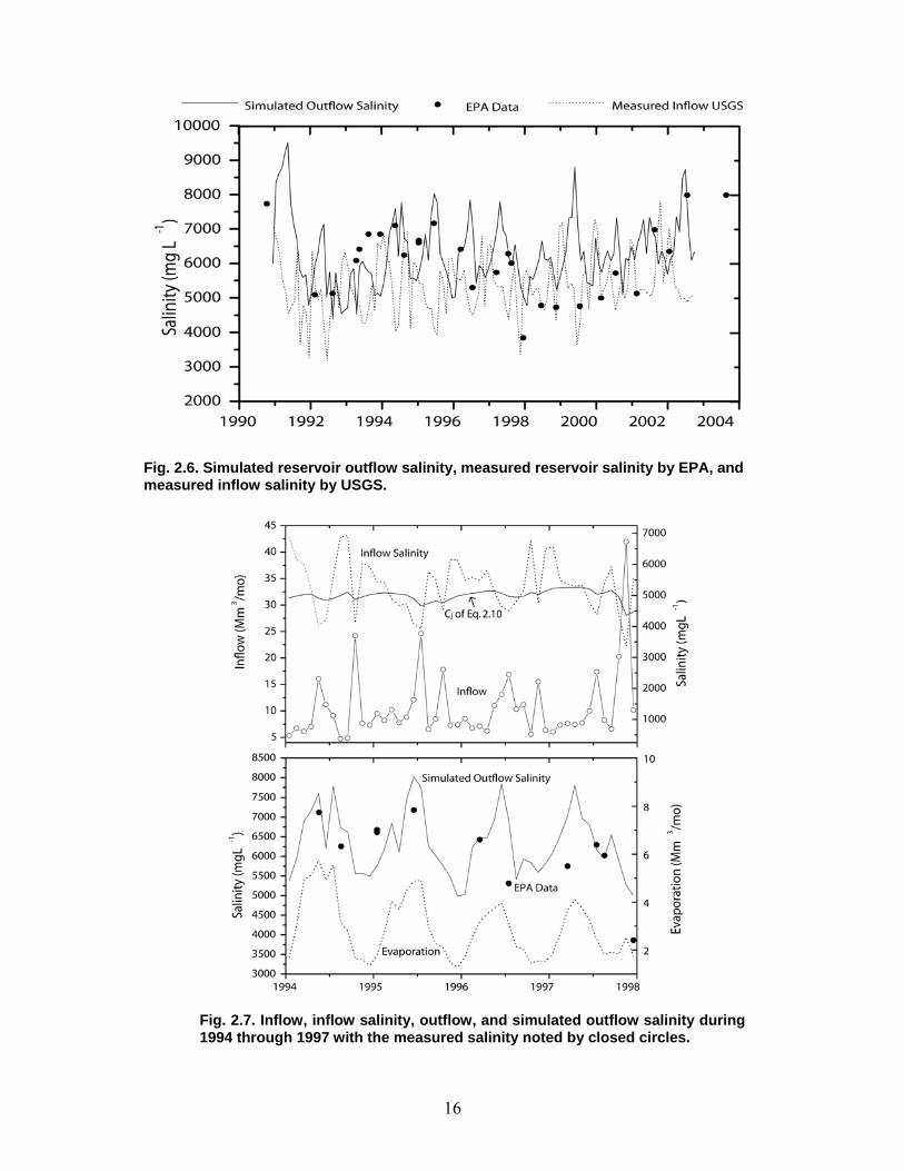
Salinity of the outflow simulated by Eq. 1.2.3 is shown by the solid line in Fig. 2.6. The depth of the top layer (d of Eq. 1.2.4) was found to be 0.8 m (2.6 ft) through numerical matching. Salinity of the inflow (USGS data at the Pecos plus the DWR) recorded is shown by the dotted line, and averaged 5360 mg L-1 (arithmetic mean) or 4425 mg L-1 (flow-weighted mean). The arithmetic mean of the EPA data taken at the inlet to Red Bluff was 5495 mg L-1, which is close to the arithmetic mean of the USGS (5360 mg L-1).

The simulation of outflow salinity by the model produced an arithmetic mean salinity of 6300 mg L-1, as compared to the measured salinity of 6150 mg L-1 by the EPA. Salinity of the reservoir near the outlet gate reported by the EPA deviated significantly from the simulated salinity for the years of 1993 and 1998/99. During 1993, the measured salinity was higher than the projected, and was similar to the projected salinity of 1992. The records in Fig. 2.6 show that the reservoir storage peaked in 1992, then decreased sharply in 1993 and 1994. It is entirely possible that the salinity measured in 1993 near

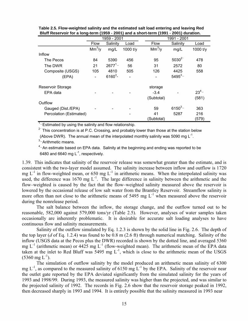
Table 2.5. Flow-weighted salinity and the estimated salt load entering and leaving Red Bluff Reservoir for a long-term (1959 - 2001) and a short-term (1991 - 2001) duration.

Flow Salinity Load Flow Salinity LoadMm3/y mg/L 1000 t/y Mm3/y mg/L 1000 t/y

Inflow The Pecos 84 5390 456 95 50302- 478 The DWR 21 26771- 56 31 2572 80 Composite (USGS) 105 4810 505 126 4425 558 (EPA) - 61603- - - 54953-

Reservoir Storage storage EPA data - - - -3.4 - 234-

(Subtotal) (581)Outflow Gauged (Dist./EPA) - - - 59 61503- 363 Percolation (Estimated) - 41 5287 216

(Subtotal) (579)

2- This concentration is at P.C. Crossing, and probably lower than those at the station below (Above DWR). The annual mean of the interpolated monthly salinity was 5090 mg L-1.

4-An estimate based on EPA data. Salinity at the beginning and ending was reported to be 6480 and 6640 mg L-1, respectively.

1959 - 2001 1991 - 2001

1-Estimated by using the salinity and flow relationship.

3-Arithmetic means.

16

Fig. 2.6. Simulated reservoir outflow salinity, measured reservoir salinity by EPA, and measured inflow salinity by USGS.

Fig. 2.7. Inflow, inflow salinity, outflow, and simulated outflow salinity during1994 through 1997 with the measured salinity noted by closed circles.

17

the outflow gate was salinity of the water stored in 1992 which had not been mixed well with the low incoming flow during 1993. In 1998 and 1999, the measured salinity was lower than the projected. The salinity of the reservoir measured at the surface near the outflow gate was similar to the salinity of inflow measured by the USGS. As shown in Fig. 2.7, a large amount of water was transferred from the Brantley to Red Bluff once at the end of 1987. This flow might have reached the outflow gate without sufficient mixing with the reservoir storage. The quantity of water released into Red Bluff in the month equaled half of the reservoir storage. Otherwise the prediction seems to be reasonable.

Fig. 2.7 shows the relationship between the inflow, the inflow salinity, and the evaporation on a monthly time scale for the period of 1994 through 1997. Note that salinity of the inflow decreased with increasing monthly inflow. Salinity fluctuation in the inflow was quite large, ranging mostly from 4,000 to 7,000 mg L-1. The low salinity corresponds approximately to salinity of the inflow originating from upstream reservoirs, namely Brantley. High inflow salinity corresponds mostly to salinity of the baseflow (returnflow and brine intrusion). Included in the figure is the salinity estimated by Eq. 1.2.3 prior to evaporative concentration. It shows stable salinity as a result of inflow mixing with the reservoir storage. Salinity of inflow decreased following reservoir release from Brantley, which took place mostly May through October or November. However, salinity of outflow from Red Bluff increased towards the summer months due to evaporative concentration of the reservoir surface layer.

2.2 Elephant Butte, Amistad, and Falcon

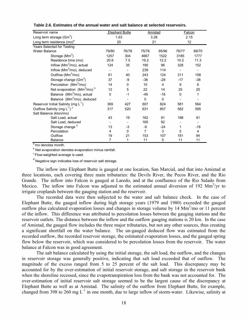
The model was tested by using inflow and outflow data from three additional reservoirs; Elephant Butte, Amistad, and Falcon, all located along the Rio Grande. These reservoirs are managed under bi-national agreements, and have extensive flow and salinity records. Elephant Butte is located in New Mexico and was completed in 1916 with the initial capacity of 2.7 Gm3 (2.19 million acre-ft). The residence time since 1975 averaged 20 months (Table 2.6). Amistad International Reservoir, completed in 1968, has the maximum storage capacity of 6.9 Gm3 (5.6 million acre-ft), but the actual storage since 1969 averaged 3.3 Gm3 (2.7 million acre-ft). Falcon Reservoir has a storage capacity of 3.9 Gm3 (3.16 million acre-ft) and the mean storage was 2.1 Gm3 (1.7 million acre-ft) since 1969. The residence time of both reservoirs fluctuated widely: 1 to 75 months, with an average of 21 and 12 months for Amistad and Falcon, respectively. The monthly evaporation accounts for 12 to 20 percent of the inflow into these reservoirs. 2.2.1 Data Used and Computational Procedures

Streamflow and salinity data below Elephant Butte were obtained from the US-IBWC and those above Elephant Butte from the U.S. Bureau of Reclamation. Salinity data were derived from the electrical conductivity using conversion factors assigned to various gauging stations (Miyamoto et al.,1995). The conductivity records were available daily at several key gauging stations, and once a week at some locations. Evaporation data at Elephant Butte were downloaded from the National Climatic Data Center, and those at Amistad and Falcon reservoirs estimated from the pan evaporation data obtained at several stations nearby. The pan coefficient of 0.70 was used to estimate evaporative water loss from the reservoir, following the calibration made by the Texas Water Development Board. The pan coefficient of 0.70 was also found suitable in the other studies (Khan and Bohra, 1990).

The flow and salinity data were screened for testing, based primarily on two criteria: i) availability of salinity data which were taken at least twice a week, and ii) at least 12 consecutive months of high or low storage. These criteria are arbitrary, but were used mainly to assure quality of the salinity data under two different storage regimes. Examples of the data set used are shown in Table 2.6. Additional data used for testing were high and low storage periods at Amistad (January 1978 through December 1979 and January 1999 through December 2000), and high storage periods (May 1973 through April 1975 and January 1980 through March 1981) at Falcon.

18

The inflow into Elephant Butte is gauged at one location, San Marcial, and that into Amistad at three locations, each covering three main tributaries: the Devils River, the Pecos River, and the Rio Grande. The inflow into Falcon is gauged at Laredo, and at the confluence of the Rio Salado from Mexico. The inflow into Falcon was adjusted to the estimated annual diversion of 192 Mm3/yr to irrigate croplands between the gauging station and the reservoir.

The recorded data were then subjected to the water and salt balance check. In the case of Elephant Butte, the gauged inflow during high storage years (1979 and 1980) exceeded the gauged outflow plus calculated evaporation losses and changes in storage volume by 14 Mm3/mo or 11 percent of the inflow. This difference was attributed to percolation losses between the gauging stations and the reservoir outlets. The distance between the inflow and the outflow gauging stations is 20 km. In the case of Amistad, the gauged flow includes the three major tributaries, but not any other sources, thus creating a significant shortfall on the water balance. The un-gauged deduced flow was estimated from the recorded outflow, the recorded reservoir storage, the estimated evaporation losses, and the gauged spring flow below the reservoir, which was considered to be percolation losses from the reservoir. The water balance at Falcon was in good agreement.

The salt balance calculated by using the initial storage, the salt load, the outflow, and the changes in reservoir storage was generally positive, indicating that salt load exceeded that of outflow. The magnitude of the excess ranged from 5 to 25 percent of the salt load. This discrepancy may be accounted for by the over-estimation of initial reservoir storage, and salt storage in the reservoir bank when the shoreline recessed, since the evapotranspiration loss from the bank was not accounted for. The over-estimation of initial reservoir salt storage seemed to be the largest cause of the discrepancy at Elephant Butte as well as at Amistad. The salinity of the outflow from Elephant Butte, for example, changed from 398 to 260 mg L-1 in one month, due to large inflow of storm-water. Likewise, salinity at

79/80 76/78 75/76 95/96 76/771257 304 4667 1522 318520.6 7.5 19.2 12.2 10.2124 35 190 96 328

- - 239 114 -61 40 243 124 31137 -9 -36 -28 -1714 0 10 4 912 5 22 14 250 -1 -49 -18 0- - 0 0 -

369 427 607 824 581317 520 631 857 582

43 19 162 91 198- - 165 92 -

13 -3 -9 -24 14 0 7 3 5

Outflow 19 21 153 107 181Balance 7 1 11 5 11

a mo denotes month.b Net evaporation denotes evaporation minus rainfall.c Flow-weighted average is used.d Negative sign indicates loss of reservoir salt storage.

Reservoir name Elephant Butte Amistad FalconLong term storage (Gm3) 1.63 3.28 2.15Long term residence (mo)a 20 21 12Years Selected for Testing Water Balance 69/70

Storage (Mm3) 1777Residence time (mo) 11.3Inflow (Mm3/mo), actual 152Inflow (Mm3/mo), deduced -Outflow (Mm3/mo) 158Storage change (Gm3) -38Percolation (Mm3/mo) 6Net evaporation (Mm3/mo) b 25Balance (Mm3/mo), actual 1Balance (Mm3/mo), deduced -

Reservoir Initial Salinity (mg L-1) 564Outflow Salinity (mg L-1) c 595Salt Balance (kton/mo)

Salt Load, actual 91Salt Load, deduced -

9411

Storage change d -18Percolation 4

Table 2.6. Estimates of the annual water and salt balance at selected reservoirs.

19

Amistad decreased from 607 to 497 mg L-1 during the initial period. If the lower salinity readings were used as the initial storage, the salt balance was nearly zero. In the case of Falcon, salinity data from the Rio Salado from Mexico were limited, and could have affected the balance estimate.

The concentration of the initial reservoir storage was assumed to be equal to salinity of the outflow. Salinity of subsequent months was then computed as a moving average, and the empirical coefficients determined through the best fit. The computed salinity of outflow was then compared to the measured, and the standard error of the estimate computed. The empirical coefficients determined for each data set were then averaged, and salinity of the outflow was recalculated using the mean value in order to appraise the sensitivity of the salinity projection. 2.2.2 Results and Discussion

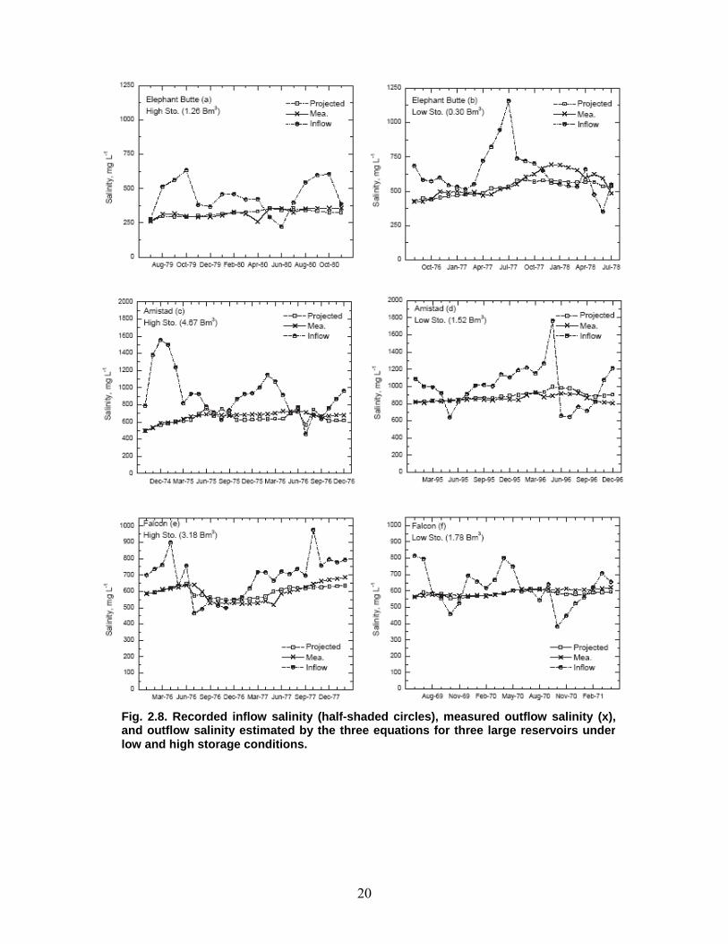
Monthly salinity of the incoming flow into the reservoirs fluctuated widely (Fig. 2.8). Inflow salinity during the low storage periods was often higher than the salinity during the high storage periods, and fluctuated just as much as it did during the high storage periods. As hypothesized at the onset, outflow salinity fluctuated to a lesser extent than did inflow salinity in all cases tested. The applicability of the model differed somewhat depending on the reservoirs tested. Elephant Butte: Salinity of the inflow into Elephant Butte during 1979 and 1980 (high storage period) varied from 220 to 600 mg L-1 (Fig. 2.8a), and salinity during 1976 and 1977 (low storage period) fluctuated between 350 and 1150 mg L-1 (Fig. 2.8b). Salinity measured in the outflow from Elephant Butte ranged from 260 to 350 mg L-1 during the high storage period, and 400 to 700 mg L-1 during the low storage period. It is evident that reservoir storage effectively buffered salinity fluctuation during both high and low storage periods.

The two-layer model provided a good estimate of outflow salinity. However, the depth of influence (d), which serves as a matching factor, was different between the high and the low storage periods. The low value of d indicates that Eq. 1.1.3 underestimated outflow salinity unless the evaporative concentration is amplified. Recall that the initial salinity of the reservoir during the high storage period was conceivably overestimated. This means that the depth factor during the high storage period must be small. The standard error of the estimate was similar for the high and the low storage periods, and was mostly less than 10 percent (Table 2.7). Amistad: Salinity of the inflow fluctuated widely between 500 and 1550 mg L-1 during the high storage period (Fig. 2.8c), and between 650 and 1800 mg L-1 during the low storage period (Fig. 2.8d). The measured salinity of outflow began at 500 mg L-1, and steadily increased to 700 mg L-1 during the high flow period, and remained around 800 mg L-1 during the low storage period (Fig. 2.8c and 2.8d).

The estimate of outflow salinity by Eq. 1.2.3, using the deduced flow, produced a low value for d during the period of 1974 through 1976. As for the case of Elephant Butte, the overestimation of the initial reservoir salt storage is likely to be the cause. The standard error was still less than 10 percent (Table 2.7). Falcon: Salinity of the inflow into this reservoir fluctuated between 400 to 1000 mg L-1, whereas salinity of the outflow varied from 550 to 650 mg L-1 (Fig. 3.1e, and 3.1f). Eq. 1.2.3 provided good estimates of the outflow salinity with the standard error of less than 5 percent, except for the period of 1973 through 1975 (Table 2.7). During this period, high outflow salinity was reported for a few months before or after flood events. It is possible that salt flushing has occurred, but was not detected during the routine salinity measurements. In any case, these discrepancies might have produced the high standard errors.

20

Fig. 2.8. Recorded inflow salinity (half-shaded circles), measured outflow salinity (x), and outflow salinity estimated by the three equations for three large reservoirs underlow and high storage conditions.

21

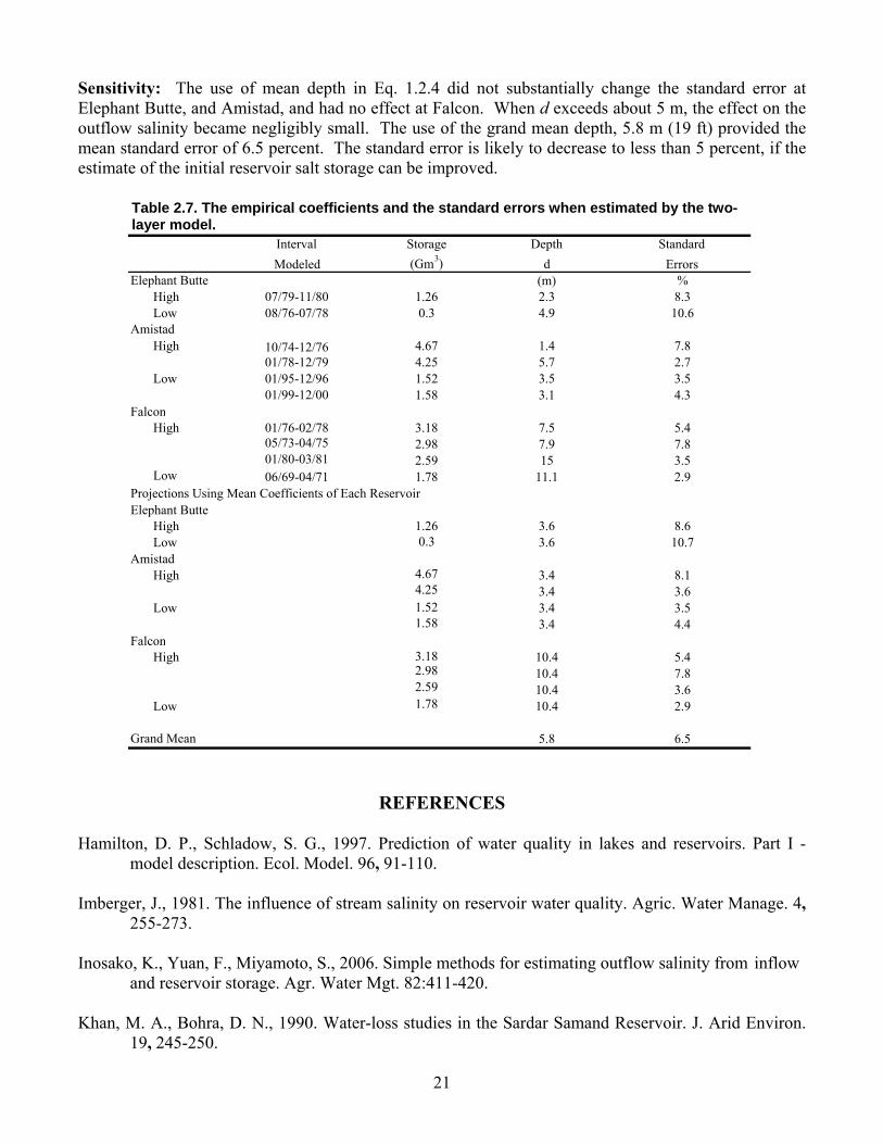
Sensitivity: The use of mean depth in Eq. 1.2.4 did not substantially change the standard error at Elephant Butte, and Amistad, and had no effect at Falcon. When d exceeds about 5 m, the effect on the outflow salinity became negligibly small. The use of the grand mean depth, 5.8 m (19 ft) provided the mean standard error of 6.5 percent. The standard error is likely to decrease to less than 5 percent, if the estimate of the initial reservoir salt storage can be improved.

REFERENCES

Hamilton, D. P., Schladow, S. G., 1997. Prediction of water quality in lakes and reservoirs. Part I -

model description. Ecol. Model. 96, 91-110. Imberger, J., 1981. The influence of stream salinity on reservoir water quality. Agric. Water Manage. 4,

255-273. Inosako, K., Yuan, F., Miyamoto, S., 2006. Simple methods for estimating outflow salinity from inflow

and reservoir storage. Agr. Water Mgt. 82:411-420. Khan, M. A., Bohra, D. N., 1990. Water-loss studies in the Sardar Samand Reservoir. J. Arid Environ.

19, 245-250.

Table 2.7. The empirical coefficients and the standard errors when estimated by the two-layer model.

Interval Storage Depth StandardModeled (Gm3) d Errors

Elephant Butte (m) % High 07/79-11/80 1.26 2.3 8.3Low 08/76-07/78 0.3 4.9 10.6

Amistad High 10/74-12/76 4.67 1.4 7.8

01/78-12/79 4.25 5.7 2.7Low 01/95-12/96 1.52 3.5 3.5

01/99-12/00 1.58 3.1 4.3Falcon

High 01/76-02/78 3.18 7.5 5.405/73-04/75 2.98 7.9 7.801/80-03/81 2.59 15 3.5

Low 06/69-04/71 1.78 11.1 2.9

High 1.26 3.6 8.6Low 0.3 3.6 10.7

Amistad High 4.67 3.4 8.1

4.25 3.4 3.6Low 1.52 3.4 3.5

1.58 3.4 4.4Falcon

High 3.18 10.4 5.42.98 10.4 7.82.59 10.4 3.6

Low 1.78 10.4 2.9

5.8 6.5Grand Mean

Projections Using Mean Coefficients of Each ReservoirElephant Butte

22

Killworth, P. D., Carmack, E. C., 1979. A filling-box model of river-dominated lakes. Limnol.

Oceanogr. 24, 201-217. Miyamoto, S., Switlik, D., Fenn, L. B., 1995. Flow, salts, and trace elements in the Rio Grande: A

review, p. 30. Texas Agricultural Experiment Station, The Texas A&M University System, College Station, Texas.

Miyamoto, S., Yuan, F., McDonald, A., Hatler, W., Anaya, G., Belzer, W., 2005. Reconnaissance

survey of salt sources and loading into the Pecos River. Texas A&M University Agricultural Research Center at El Paso, TX and Texas Water Resources Institute, College Station, TX, TR-291.

Zagona, E. A., Goranflo, H. M., Fulp, T. J., Shane, R., Magee, T., 2001. RiverWare: A generalized tool

for complex reservoir system modeling. J. Amer. Water Resour. Assoc. 37, 913-929.