Embed Size (px)
Citation preview
A Simple Method for High-Lift Propeller Conceptual Design
5 January 2016
Michael Patterson, Nick Borer,
NASA Langley Research Center
and Brian German
Georgia Institute of Technology
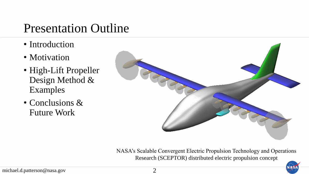
Presentation Outline
• Introduction
• Motivation
• High-Lift Propeller Design Method & Examples
• Conclusions & Future Work
2
NASA’s Scalable Convergent Electric Propulsion Technology and Operations
Research (SCEPTOR) distributed electric propulsion concept

Introduction

Electric motors enable propellers to be installed in non-traditional, beneficial manners• Electric motors have distinctly
different characteristics than conventional engines• Lower weight and volume
• Reduced vibration
• Nearly “scale-invariant”
• Wing tip props can reduce induced drag / increase propulsive efficiency
• “High-lift props” placed upstream of a wing can increase lift
• Others…
4
[NASA TR-1263, 1956]
[NASA TP-2739,
1987]

Effect of prop slipstreams on downstream wings is complex, but can be approximated with a simple model• Propellers induce axial and
tangential (“swirl”) velocities
• High-lift props alter the zero-lift angle of attack and lift curve slope of downstream wing sections
• Wing upwash impacts inflow to prop disk
• To first-order, prop impacts on lift can be assessed via a single, average induced axial velocity
→Small wing impacts on prop
→Swirl affects on either side of disk “cancel out”
5
Notional propeller swirl
velocity profile
ivV 2ivV
V
T
Prop
Induced axial velocity increase as
predicted by momentum theory
Typical induced
axial velocity profile
MotivationShould high-lift propellers be designed in the same
manner as conventional propellers?

Because the goal of high-lift props differs from conventional props, they should be designed differently
• Goal of conventional props is to produce thrust, but goal of high-lift props is to augment lift• Thrust may actually be bad for high-lift props!
• Props primarily affect lift via induced velocity
• Chow et al. indicate that the axial velocity profile affects the lift generated• Placed Joukowski velocity profiles upstream of
airfoil and studied lift generated
• Varied airfoil height relative to profile
• Define “non-uniformity parameter”: a/d2
• Define “adjusted lift coefficient”:
7
[Chow 1970, DOI 10.2514/3.44208]
𝑉 𝑧 = 𝑉∞ 1 + 𝑎𝑒−𝑧2/𝑑2
𝐶𝐿 =𝐶𝐿
(1 + 𝑎)2
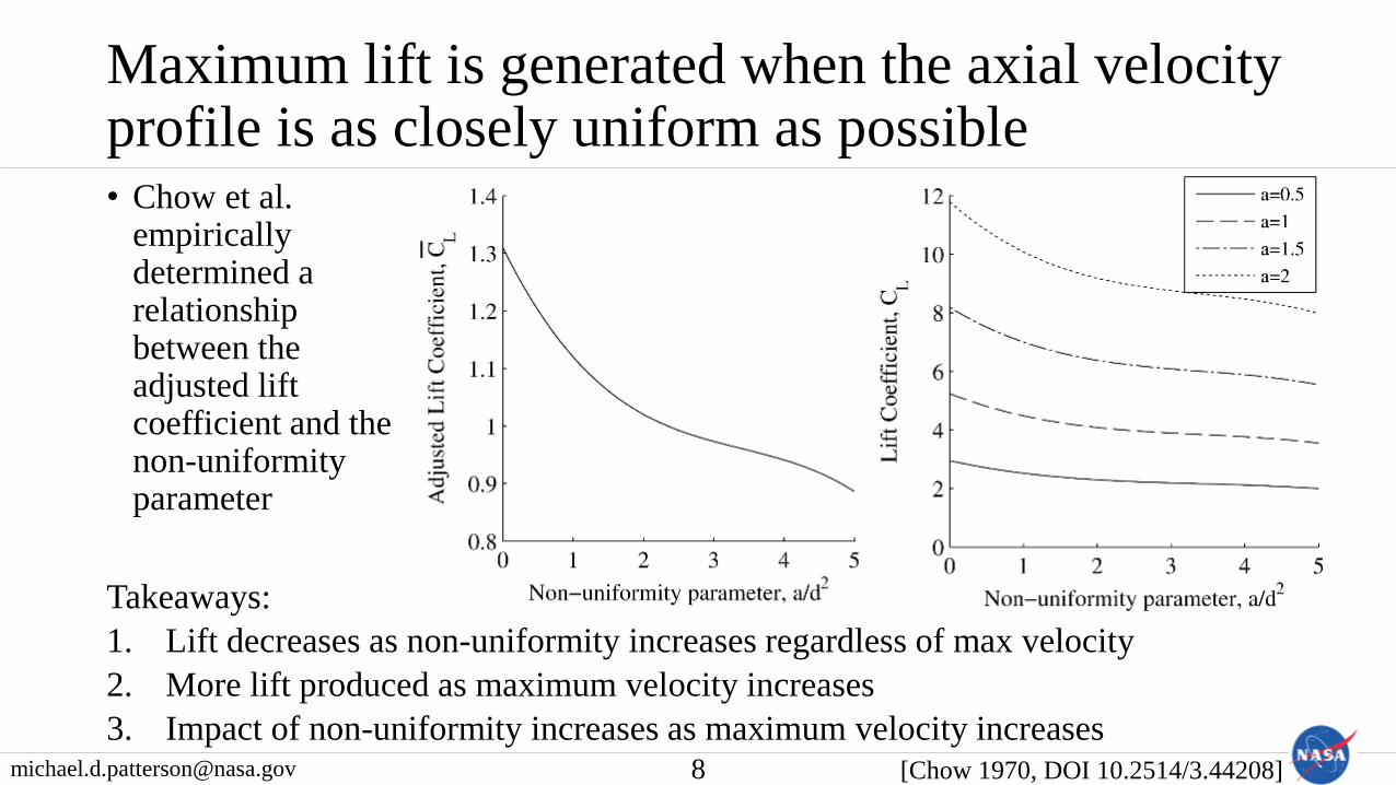
Maximum lift is generated when the axial velocity profile is as closely uniform as possible
Takeaways:
1. Lift decreases as non-uniformity increases regardless of max velocity
2. More lift produced as maximum velocity increases
3. Impact of non-uniformity increases as maximum velocity increases8 [Chow 1970, DOI 10.2514/3.44208]
• Chow et al. empirically determined a relationship between the adjusted lift coefficient and the non-uniformity parameter
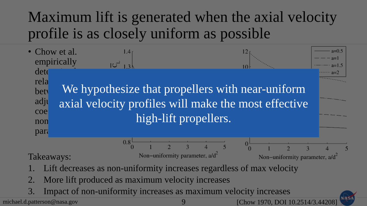
Maximum lift is generated when the axial velocity profile is as closely uniform as possible
Takeaways:
1. Lift decreases as non-uniformity increases regardless of max velocity
2. More lift produced as maximum velocity increases
3. Impact of non-uniformity increases as maximum velocity increases9 [Chow 1970, DOI 10.2514/3.44208]
• Chow et al. empirically determined a relationship between the adjusted lift coefficient and the non-uniformity parameter
We hypothesize that propellers with near-uniform
axial velocity profiles will make the most effective
high-lift propellers.

High-Lift Propeller Design Method & Examples
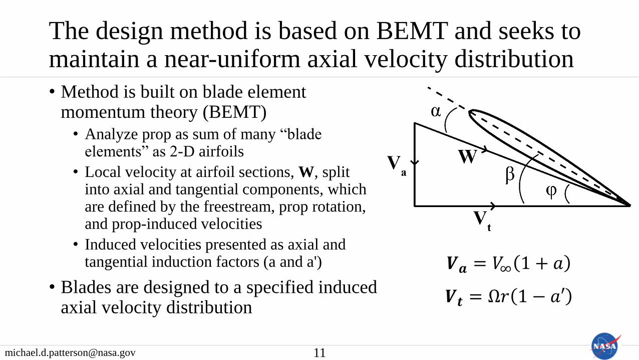
The design method is based on BEMT and seeks to maintain a near-uniform axial velocity distribution
• Method is built on blade element momentum theory (BEMT)
• Analyze prop as sum of many “blade elements” as 2-D airfoils
• Local velocity at airfoil sections, W, split into axial and tangential components, which are defined by the freestream, prop rotation, and prop-induced velocities
• Induced velocities presented as axial and tangential induction factors (a and a')
• Blades are designed to a specified induced axial velocity distribution
11
𝑽𝒂 = 𝑉∞ 1 + 𝑎
𝑽𝒕 = Ω𝑟 1 − 𝑎′

The design method consists of four steps, where the first is the most important and novel• Assumptions:
• Designer desires constant induced axial velocity distribution
• The diameter, number of blades, rotational speed, and airfoil(s) are known
• The angular velocity added to the slipstream is small compared to the angular velocity of the propeller
• Steps in method:1. Set axial induction factor distribution
2. Determine blade pitch angle distribution
3. Determine blade chord length distribution
4. Verify performance and iterate (if required)
12
𝑽𝒂 = 𝑉∞ 1 + 𝑎
𝑽𝒕 = Ω𝑟 1 − 𝑎′

Steps 1-3: Setting the axial induction factor distribution determines the blade chord/pitch distributions
• Begin by specifying a constant axial velocity distribution based on desired average induced velocity
• If assumptions are valid, then axial and tangential induction factors are related
• Relationship implies maximum value for a' as 0.5
• If desired value of a leads to a' > 0.5, limit a' to 0.5
• If limiting a', find new implied value of a
13
𝑉∞2 1 + 𝑎 𝑎 = Ω2𝑟2 1 − 𝑎′ 𝑎′
𝑎 =𝑣𝑖𝑉∞
𝑎′ =1 − 1 −
4𝑉∞2 1 + 𝑎 𝑎Ω2𝑟2
2
𝑎 =
−1 + 1 +4Ω2𝑟2 1 − 𝑎′ 𝑎′
𝑉∞2
2

Step 4: Verify prop performance and iterate (if required) until desired average induced axial velocity is achieved
• Average induced axial velocity from method will likely not match desired value (due to assumptions, hub/tip losses, limiting a', etc.)
• We utilize XROTOR in vortex mode to verify average axial velocity
• XROTOR is open-source prop design/analysis tool from Mark Drela’sresearch group at MIT
• If average induced axial velocity is too low (high), increase (decrease) induced axial velocity specified in Step 1 and repeat
• In practice, found that approximately 2-3 iterations are required for convergence
14
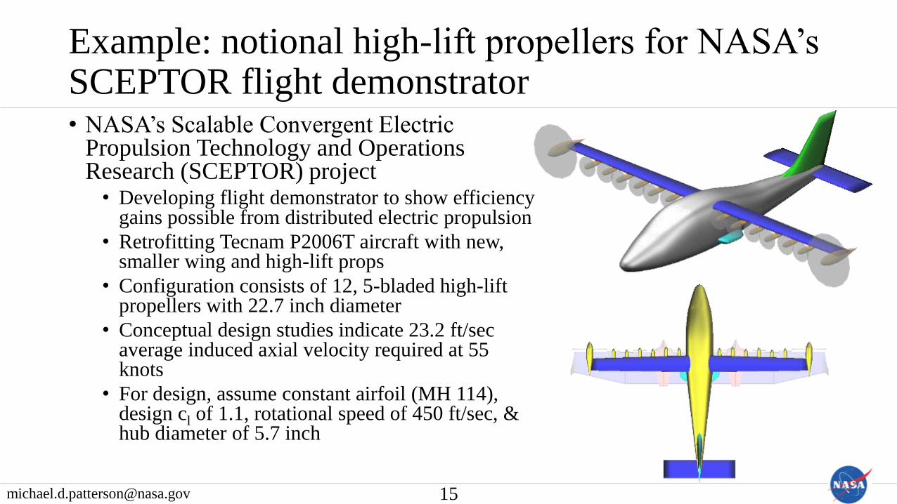
Example: notional high-lift propellers for NASA’s SCEPTOR flight demonstrator• NASA’s Scalable Convergent Electric
Propulsion Technology and Operations Research (SCEPTOR) project• Developing flight demonstrator to show efficiency
gains possible from distributed electric propulsion
• Retrofitting Tecnam P2006T aircraft with new, smaller wing and high-lift props
• Configuration consists of 12, 5-bladed high-lift propellers with 22.7 inch diameter
• Conceptual design studies indicate 23.2 ft/sec average induced axial velocity required at 55 knots
• For design, assume constant airfoil (MH 114), design cl of 1.1, rotational speed of 450 ft/sec, & hub diameter of 5.7 inch
15

A conventional, minimum induced loss (MIL) prop was designed via XROTOR for the SCEPTOR aircraft
16
Isometric View
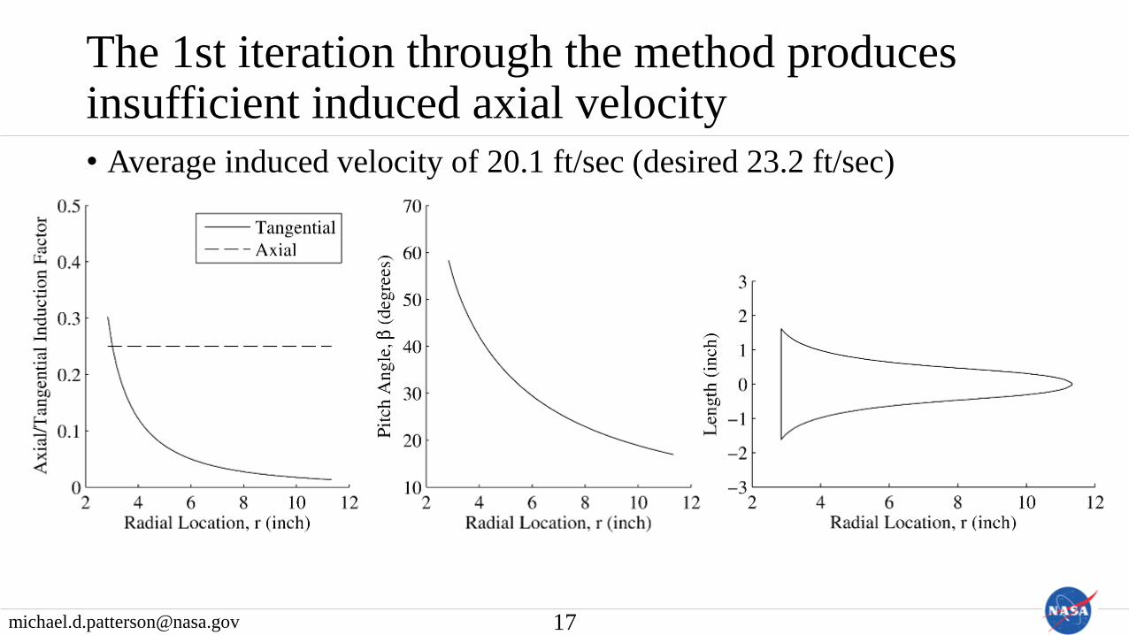
The 1st iteration through the method produces insufficient induced axial velocity
• Average induced velocity of 20.1 ft/sec (desired 23.2 ft/sec)
17
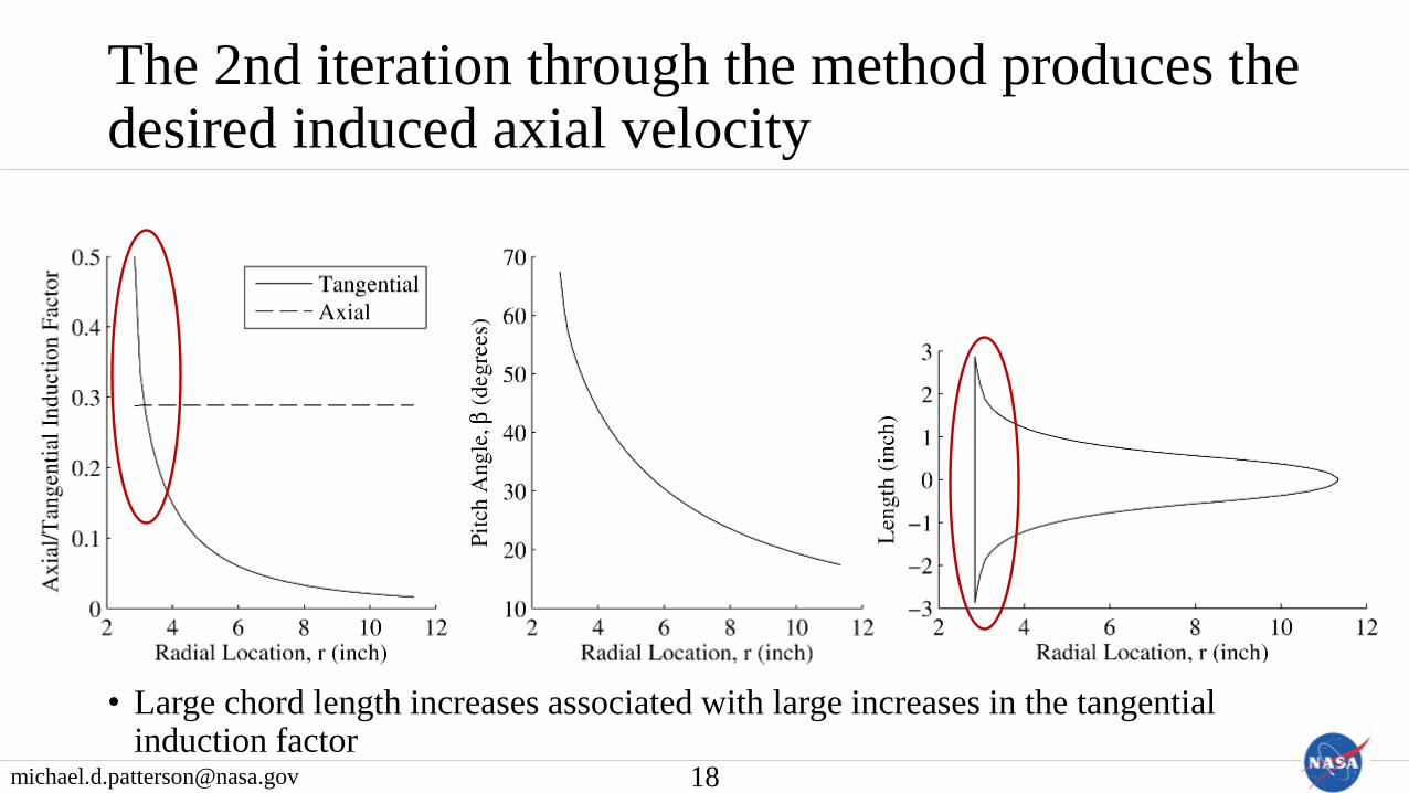
The 2nd iteration through the method produces the desired induced axial velocity
• Large chord length increases associated with large increases in the tangential induction factor
18
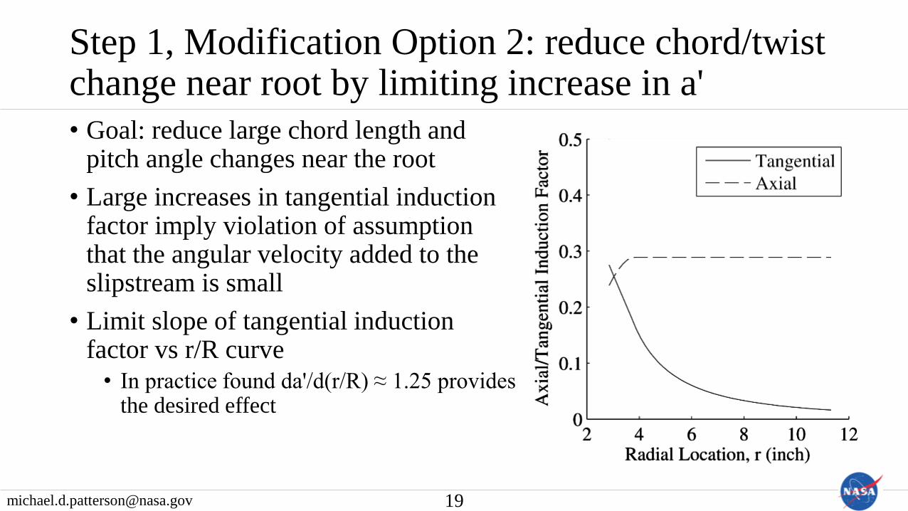
Step 1, Modification Option 2: reduce chord/twist change near root by limiting increase in a'
• Goal: reduce large chord length and pitch angle changes near the root
• Large increases in tangential induction factor imply violation of assumption that the angular velocity added to the slipstream is small
• Limit slope of tangential induction factor vs r/R curve
• In practice found da'/d(r/R) ≈ 1.25 provides the desired effect
19
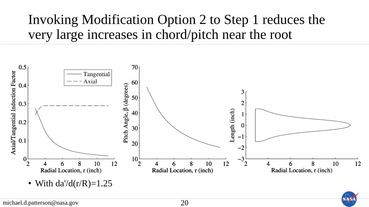
Invoking Modification Option 2 to Step 1 reduces the very large increases in chord/pitch near the root
• With da'/d(r/R)=1.25
20
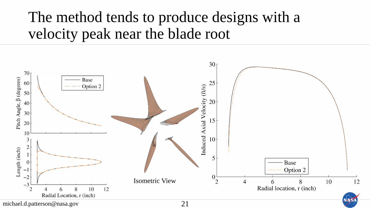
The method tends to produce designs with a velocity peak near the blade root
21
Isometric View

Step 1, Modification Option 1: applying modified Prandtltip loss factor to a provides desired blade loading at tip
• Modify tip loss factor with larger radius
• Found R'=1.035R provides desired results
22
𝐹 =2
𝜋cos−1[𝑒
−𝐵2
(𝑅′−𝑟)𝑟 sin 𝜑 ] 𝑎𝑚𝑜𝑑 =
𝑎
𝐹
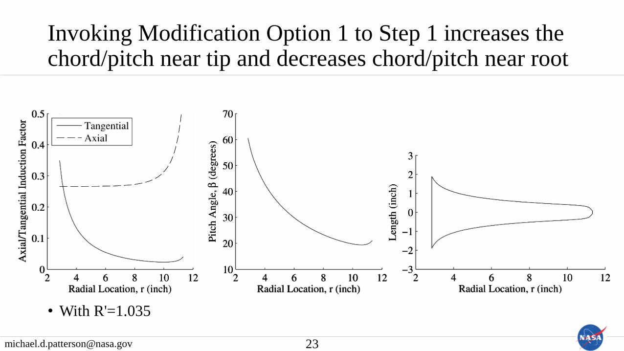
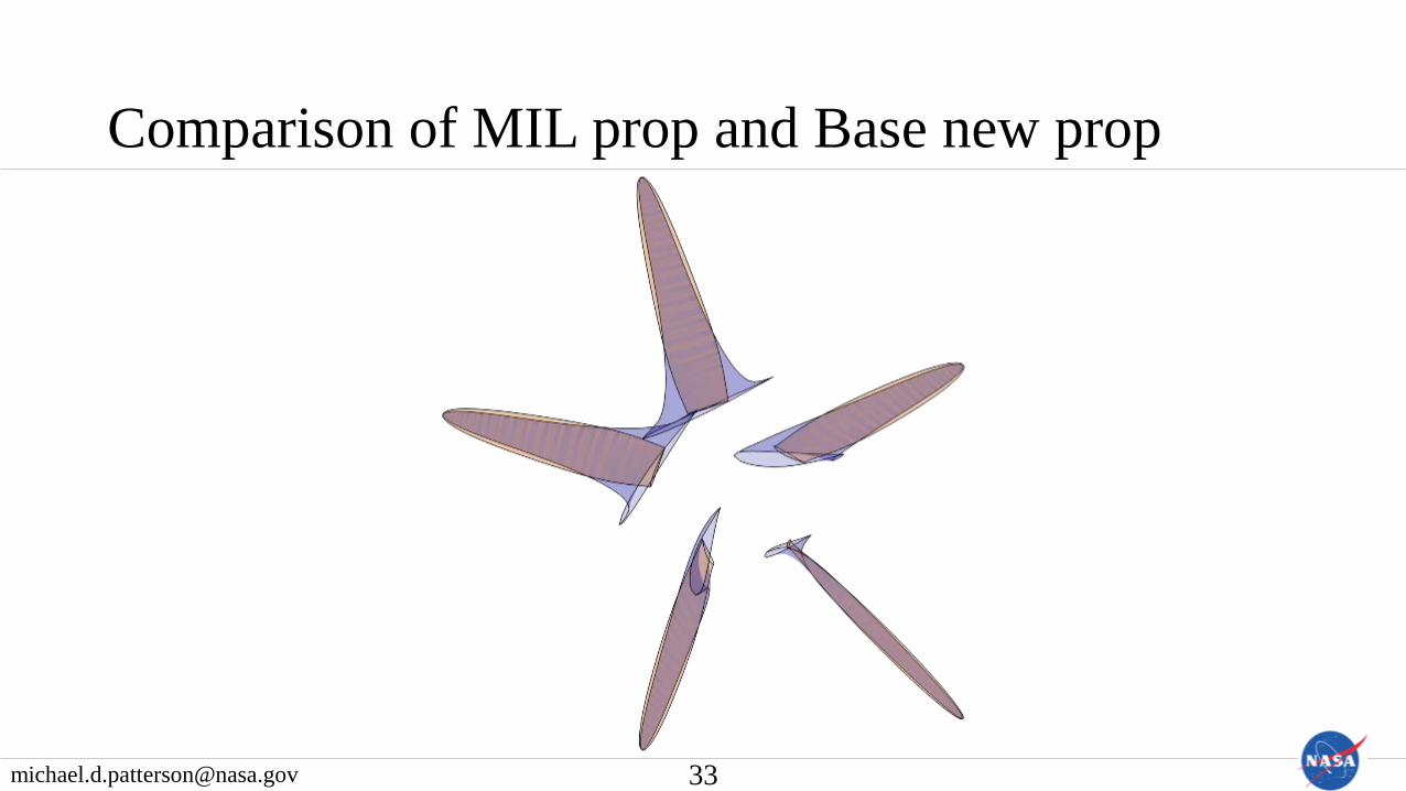
Invoking Modification Option 1 to Step 1 increases the chord/pitch near tip and decreases chord/pitch near root
• With R'=1.035
23
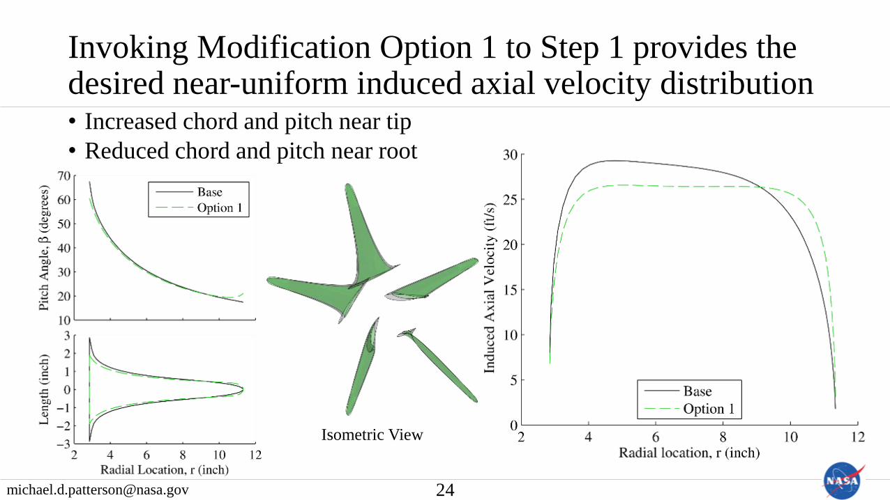
• Increased chord and pitch near tip
• Reduced chord and pitch near root
Invoking Modification Option 1 to Step 1 provides the desired near-uniform induced axial velocity distribution
24
Isometric View

• Slight decrease in induced axial velocity near root
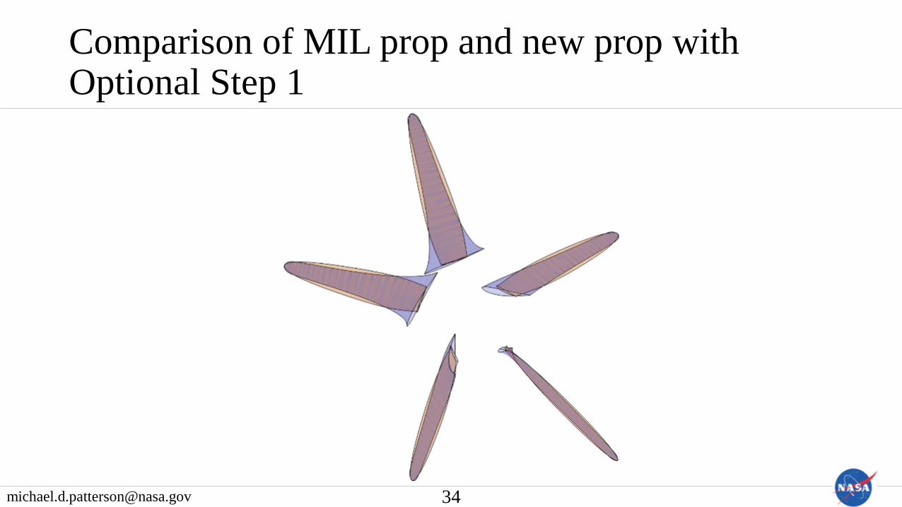
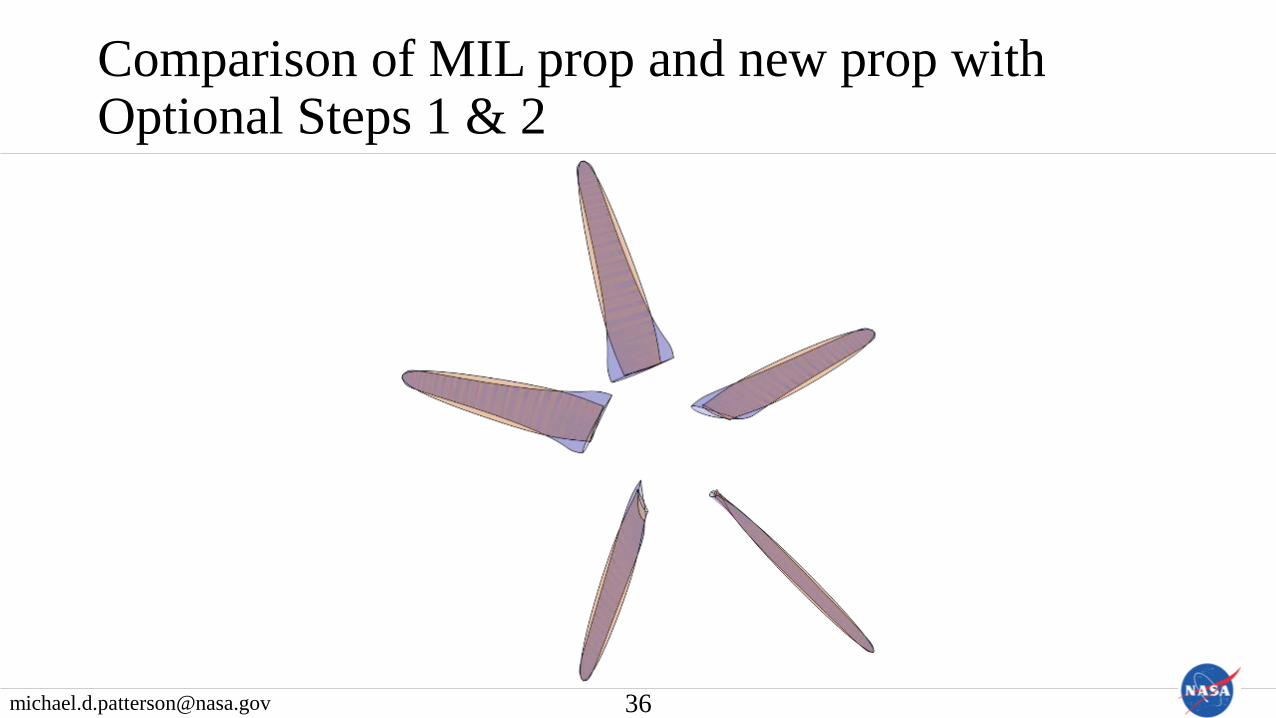
Modification Options 1 & 2 when invoked simultaneously produce near-uniform velocities & reasonable blade shapes
25
Isometric View

Design method produces props with much more uniform velocity distributions than conventional props
26
Isometric View
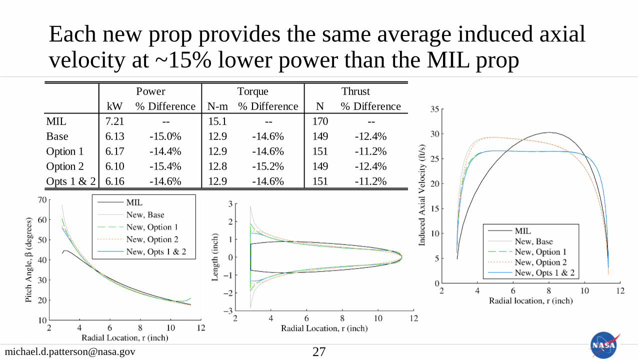
Each new prop provides the same average induced axial velocity at ~15% lower power than the MIL prop
27
kW % Difference N-m % Difference N % Difference
MIL 7.21 -- 15.1 -- 170 --
Base 6.13 -15.0% 12.9 -14.6% 149 -12.4%
Option 1 6.17 -14.4% 12.9 -14.6% 151 -11.2%
Option 2 6.10 -15.4% 12.8 -15.2% 149 -12.4%
Opts 1 & 2 6.16 -14.6% 12.9 -14.6% 151 -11.2%
Power Torque Thrust

Conclusions & Future Work
The new prop designs are predicted to augment more lift than traditional props for a given power• Recall hypothesis: propellers with near-uniform axial velocity profiles will
make the most effective high-lift propellers
• Conclusions• Design method produces the desired near-uniform induced axial velocity profile
• Design method produces high-lift props with ~15% lower powers and ~11% lower thrusts than traditional methods to produce the same average induced axial velocity
• Future work• Wind tunnel testing and/or unsteady CFD are required to validate performance
predictions
• Consider removing assumption that the rotational velocity added to the slipstream is small
• Study impacts of large pitch angles near root on blade folding
• Study impacts of varying airfoils along blade
• Aeroelastic analysis
29

Questions?This work was funded under the Convergent Aeronautics
Solutions (CAS) and Transformational Tools and Technologies (TTT) Projects of NASA’s Transformative Aeronautics
Concepts Program.

Backup
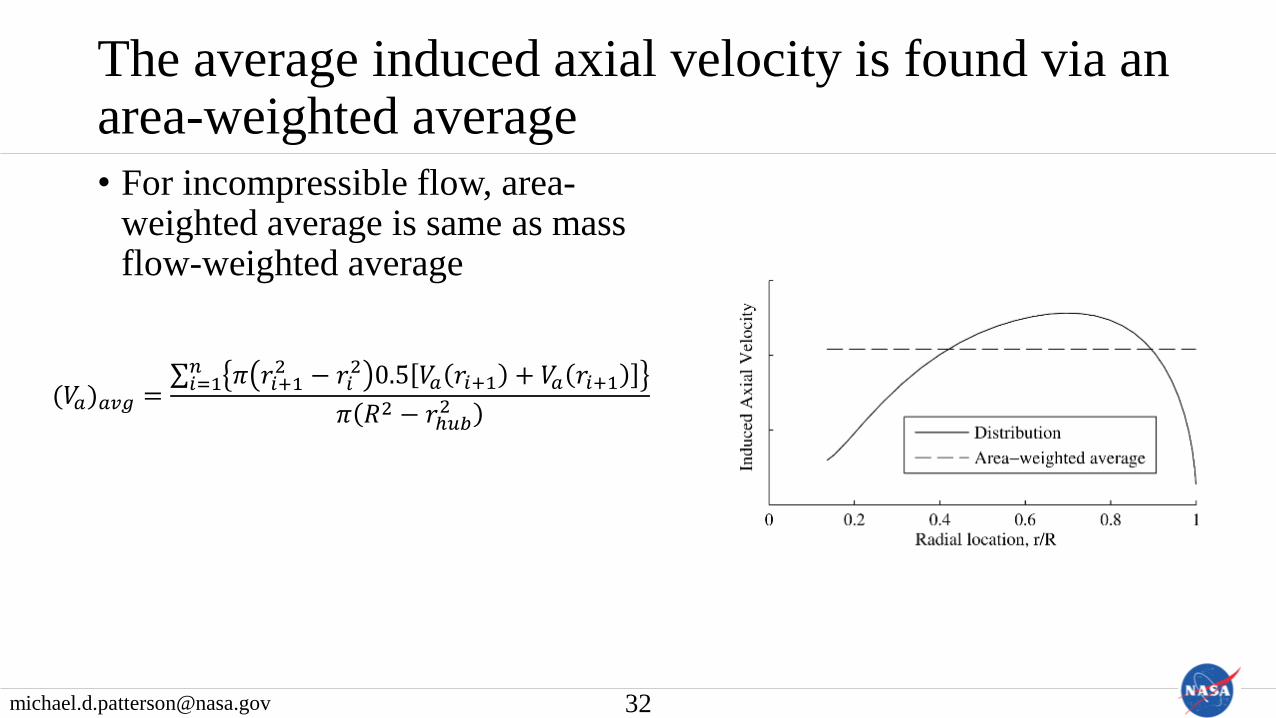
The average induced axial velocity is found via an area-weighted average
• For incompressible flow, area-weighted average is same as mass flow-weighted average
32
(𝑉𝑎)𝑎𝑣𝑔 = 𝑖=1𝑛 𝜋 𝑟𝑖+1
2 − 𝑟𝑖2 0.5 𝑉𝑎 𝑟𝑖+1 + 𝑉𝑎 𝑟𝑖+1
𝜋 𝑅2 − 𝑟ℎ𝑢𝑏2

The design method is based on BEMT and seeks to maintain a near-uniform axial velocity distribution• Method is built on blade element momentum
theory (BEMT) • Analyze prop as sum of many “blade elements”
as 2-D airfoils• Local velocity split into axial and tangential
components, which are defined by the freestream, prop rotation, and prop-induced velocities
• Induced velocities presented as axial and tangential induction factors (a and a')
• We assume that the angular velocity added to the slipstream is small compared to the angular velocity of the propeller
• Method has four main steps:1. Set axial induction factor distribution2. Determine blade twist angle distribution3. Determine blade chord length distribution4. Verify performance and iterate (if required)
37
𝑽𝒂 = 𝑉∞ 1 + 𝑎
𝑽𝒕 = Ω𝑟 1 − 𝑎′
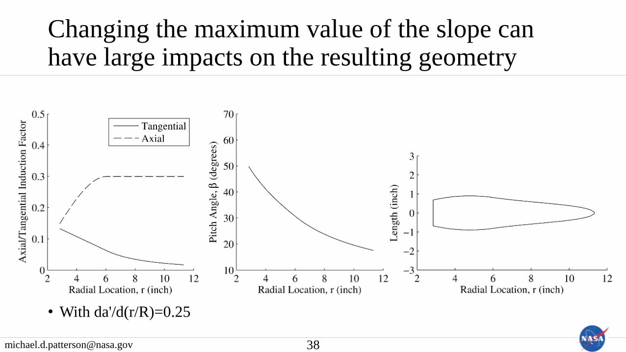
Changing the maximum value of the slope can have large impacts on the resulting geometry
• With da'/d(r/R)=0.25
38
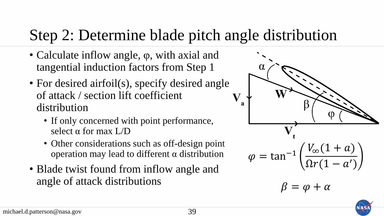
Step 2: Determine blade pitch angle distribution
• Calculate inflow angle, φ, with axial and tangential induction factors from Step 1
• For desired airfoil(s), specify desired angle of attack / section lift coefficient distribution
• If only concerned with point performance, select α for max L/D
• Other considerations such as off-design point operation may lead to different α distribution
• Blade twist found from inflow angle and angle of attack distributions
39
𝜑 = tan−1𝑉∞(1 + 𝑎)
Ω𝑟(1 − 𝑎′)
𝛽 = 𝜑 + 𝛼

Step 3: Determine blade chord length distribution• The thrust from an annulus of the prop
disk can be expressed in two equations• One from momentum theory and the
other blade element theory
• Only unknown is the chord length
• Equate two expressions for thrust and solve for the chord length• Assumes the airfoil aerodynamic
characteristics are known
• Number of blades must be specified
40
where
𝑑𝑇 = 4𝜋𝑟𝜌𝑉∞2 1 + 𝑎 𝑎𝐹𝑑𝑟
𝑑𝑇 =𝐵
2𝜌𝑊2 𝑐𝑙 cos 𝜑 − 𝑐𝑑sin(𝜑) 𝑐𝑑𝑟
𝐹 =2
𝜋cos−1[𝑒
−𝐵2
(𝑅−𝑟)𝑟 sin 𝜑 ]
𝑐 =8𝜋𝑟𝑉∞
2 1 + 𝑎 𝐹
𝐵𝑊2 𝑐𝑙 cos 𝜑 − 𝑐𝑑sin(𝜑)
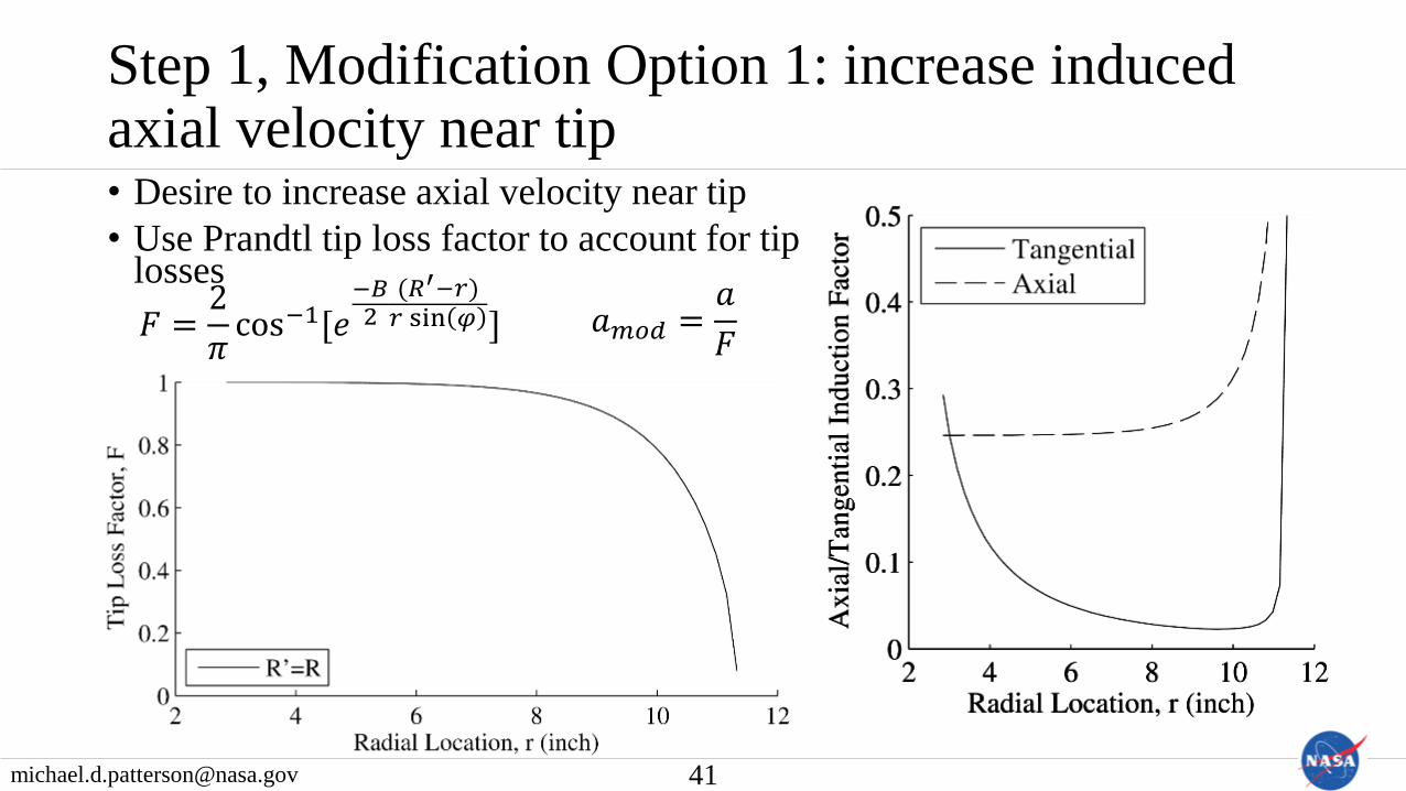
Step 1, Modification Option 1: increase induced axial velocity near tip• Desire to increase axial velocity near tip
• Use Prandtl tip loss factor to account for tip losses
41
𝐹 =2
𝜋cos−1[𝑒
−𝐵2
(𝑅′−𝑟)𝑟 sin 𝜑 ] 𝑎𝑚𝑜𝑑 =
𝑎
𝐹