A simple embedding method for solving partial differential equations on surfaces

Available online at www.sciencedirect.com

Journal of Computational Physics 227 (2008) 1943–1961

www.elsevier.com/locate/jcp

A simple embedding method for solving partialdifferential equations on surfaces

Steven J. Ruuth a,*,1, Barry Merriman b

a Department of Mathematics, Simon Fraser University, Burnaby, British Columbia, Canada V5A 1S6b University of California, Los Angeles, CA, United States

Received 13 October 2006; received in revised form 12 June 2007; accepted 3 October 2007Available online 22 October 2007

Abstract

It is increasingly common to encounter partial differential equations (PDEs) posed on surfaces, and standard numericalmethods are not available for such novel situations. Herein, we develop a simple method for the numerical solution of suchequations which embeds the problem within a Cartesian analog of the original equation, posed on the entire space con-taining the surface. This allows the immediate use of familiar finite difference methods for the discretization and numericalsolution. The particular simplicity of our approach results from using the closest point operator to extend the problemfrom the surface to the surrounding space. The resulting method is quite general in scope, and in particular allows forboundary conditions at surface boundaries, and immediately generalizes beyond surfaces embedded in R3, to objects ofany dimension embedded in any Rn. The procedure is also computationally efficient, since the computation is naturallyonly carried out on a grid near the surface of interest. We present the motivation and the details of the method, illustrateits numerical convergence properties for model problems and also illustrate its application to several complex modelequations.� 2007 Elsevier Inc. All rights reserved.

Keywords: Closest point representations; Partial differential equations; Implicit surfaces; Finite difference schemes; Manifolds; Laplace–Beltrami operator

1. Introduction

Many applications in the natural and applied sciences require the solutions of partial differential equations(PDEs) on surfaces or more general manifolds. Examples of such application areas arise in biological systems,image processing, medical imaging, mathematical physics, fluid dynamics and computer graphics. For exam-ple, applications in image processing include the generation of textures [27,28], the visualization of vector

0021-9991/$ - see front matter � 2007 Elsevier Inc. All rights reserved.

doi:10.1016/j.jcp.2007.10.009

* Corresponding author.E-mail addresses: [email protected] (S.J. Ruuth), [email protected] (B. Merriman).

1 The work of this author was partially supported by a grant from NSERC Canada.

mailto:[email protected]

mailto:[email protected]

1944 S.J. Ruuth, B. Merriman / Journal of Computational Physics 227 (2008) 1943–1961

fields [7] and weathering [8], while applications in fluid dynamics include flows and solidification on surfaces[17,18], and the problem of evolving surfactants on interfaces [29].

A popular approach to solving PDEs on surfaces is to impose a smooth coordinate system or parameter-ization on the surface, express differential operators within these coordinates, and then discretize the resultingequations. See, for example [10] for a tutorial and survey of methods for parameterizing surfaces. However,the required coordinates can be complicated or impractical to construct, and the coordinates may introduceartificial singularities, such as at the poles in spherical coordinates. Indeed, as pointed out in [10], ‘‘parame-terizations almost always introduce distortion in either angles or some region’’. Also, equations that are simplewhen written using intrinsic derivatives, such as surface diffusion, become substantially more complex whenwritten in a coordinate system, involving nonconstant coefficients and more derivative terms.

Another common approach to solving partial differential equations on surfaces is to solve the PDE directlyon a triangulation of the surface. This approach can be effective for certain classes of equations, however, as ageneral technique it leads to a number of difficulties. These are discussed in [3,4]. In particular, this approachleads to nontrivial discretization procedures for the differential operators, as well as difficulties in accuratelycomputing geometric primitives, such as surface normals and curvature [3]. In addition, convergence ofnumerical schemes on triangulated surfaces remains less well understood than methods on Cartesian grids [11].

An alternative approach to treating PDEs on surfaces is to embed the surface differential equations of inter-est within differential equations posed on all of R3, so that the solution of the embedding equations, whenrestricted to the surface, provides the solution to the original problem. With such an approach, the ultimategoal is to develop a method that allows the treatment of general, complex surface geometry, while still retain-ing the simplicity that comes from working in standard Cartesian coordinates. With this in mind, Bertalmıoet al. [3] introduced an embedding method for solving variational problems and the resulting Euler–Lagrangeevolution PDEs on surfaces. In their approach, the underlying surface is represented as the level-set of a higherdimensional function and the evolution corresponding to the surface PDEs is carried out via PDEs that areposed on all of R3. This leads to equations that can be discretized and solved using Cartesian grid methods.A further improvement to this method was proposed by Greer [11]. In his approach, the evolution equation ismodified away from the surface to maintain greater regularity of the solution near the surface of interest. Seealso [1] for related work on the finite element approximation of elliptic partial differential equations on implicitsurfaces via level-set methods.

Embedding methods based on level-set methods have a number of limitations, however. Most obviously,these methods do not immediately allow for open surfaces with boundaries, or filamentary objects of codimen-sion-two or higher, although it is in principle possible to represent such objects by introducing additional level-set functions. Another limitation is that these methods result in an embedding PDE posed on all of space, andcomplications arise when they are solved in a restricted computational band around the surface. Such ‘‘narrowbanding’’ requires the imposition of appropriate boundary conditions, and how to best impose these condi-tions is not generally understood. For example, even using the regularity improvements proposed by Greer[11], a degradation of the order of convergence is observed when banding is used in diffusive problems. Ata more technical level, level-set based methods also either lead to degenerate diffusion equations or requirethe use of an additional diffusion step when applied to parabolic equations [11].

Similar to other embedding methods, the approach we present here discretizes the partial differential equa-tions using a fixed Cartesian grid in the embedding space. However, our method is based on the use of a closestpoint representation of the surface (cf. [16]) rather than a level-set representation. In conjunction with thischange in representation, we abandon the concept of solving an embedding PDE for all time, and insteaduse the embedding PDE to advance the solution near the surface for one time step (or one stage of a Run-ge–Kutta method). This leads to a new method for solving PDEs on surfaces which has great simplicity, aswell as additional desirable features. Most importantly, the embedding PDE is the obvious analog of the sur-face PDE, and involves only the standard Cartesian differential operators. In addition, the method can treatopen surfaces and is not limited to objects of codimension-one. It also naturally allows the computation to bedone on a grid defined in a narrow band near the surface without any degradation in the order of accuracy andwithout imposing artificial boundary conditions. To distinguish our approach from other embedding proce-dures, and to emphasize its essential reliance on the closest point representation, we refer to the method asthe closest point method. As an aside, note that a special case of this procedure was introduced in our recent

S.J. Ruuth, B. Merriman / Journal of Computational Physics 227 (2008) 1943–1961 1945

paper on the diffusion-generated motion of curves on surfaces [16]. It was in this context that the generalpotential of the approach was first realized, although it occurs only as a special, simple procedure for approx-imating in-surface curvature motion according to the diffusion-generated motion algorithm.

The paper unfolds as follows. Section 2 gives the method, describes its implementation and provides ananalysis. In Section 3, we give a number of two-dimensional convergence studies to validate the method. Sec-tion 4 considers a variety of three-dimensional convergence tests and provides some examples that are relevantto biology: a Fitzhugh–Nagumo and a morphogenesis simulation. In Section 5, we give a summary and dis-cuss some of our ongoing projects in the subject. Finally, Appendix A concludes with a discussion on the com-putation of geometric quantities defined on the surface.

2. The closest point method

In this section, we describe the method as well as its motivation, analysis and implementation. We begin bydiscussing the motivation for the method and its surface representation.

2.1. The closest point representation

As part of our method, we need to rapidly and accurately extend functions defined on surfaces to a neigh-borhood of the surface. For maximal simplicity, this extension will be chosen according to the principle thatthe embedding PDE should be the natural extension of the original, i.e., we form the embedding PDE byreplacing intrinsic surface gradients with standard gradients on R3. Clearly, both evolutions cannot agreefor long times, but if we select a suitable extension the evolution of the embedding PDE will be accurate ini-tially, which will be sufficient to update the solution in time. Thus, we will select an operator, E, that extendsfunctions defined on the surface to functions defined on all of R3 in such a way that the natural extension ofthe surface PDE to all of space generates the required rates of change.

Note that the requirement that the all-space equation is the natural extension of the intrinsic surface equa-tion leads to a specific class of extension operators, namely those which extend function values to be constantalong the directions normal to the surface. To illustrate this, consider the special case of the prototype Ham-ilton–Jacobi equation defined on the surface,

ouS

otþ jjrSuSjj ¼ 0;

which we want to achieve for short times by treating the natural corresponding equation in all-space,ut + i$ui = 0. If we want both equations to agree on the surface, we need the extended function E[uS] to haveonly gradients along the surface directions, not normal to the surface. This means that E[uS] should be con-stant along the directions normal to the surface, and thus E[uS] must be the extension of uS which is constantmoving normal from the surface. While extending values constant normal to the surface may be an intuitivelydesirable property for the extension operator, this fundamental example shows it is in fact needed to obtainthe simplest form of the embedding equation.

Selecting an extension operator which produces a constant normal extension defines the method in generalterms. However, one ingredient which is critical to the simplicity of the resulting method is the means of actu-ally constructing the constant normal extension. A particularly simple, accurate and efficient method for con-stant normal extension is to make use of the ‘‘closest point’’ representation of the surface. For any point x inR3, let CP(x) denote the closest point to x in the surface S. If S is smooth, this function is well defined andsmooth near the surface. (It will generally have discontinuities away from S, at points in space that are equi-distant from multiple points on S. Such points do not interfere with the embedding PDE method here, whichultimately relies only on points near S, but they may place an upper limit on grid spacing in R3, in practice.)The closest point function provides an especially convenient representation of the surface for our purposebecause the constant normal extension operator can be defined in terms of it, simply as composition of func-tions, according to

E½uS �ðxÞ ¼ uSðCP ðxÞÞ


for any uS defined on S. Thus, what would otherwise be a construction process is reduced to standard eval-uation, which greatly streamlines both the practical implementation and the theoretical analysis of the meth-od. As a function, CP is simply a map from R3 to R3 that returns values lying in S.

Note that representing the underlying surface using the closest point function gives advantages that extendbeyond having a simple, fast and accurate extension process. With a closest point representation we enjoy theflexibility to represent both open and closed surfaces as well as surfaces without an orientation, such as aMobius strip or a Klein bottle. Also, curves or ‘‘filaments’’—objects of codimension-two or higher—are nat-urally accommodated in this representation, as are composite objects such as collections of surfaces, curvesand points. Thus, in general, the formalism places no limitations on the topology, geometry or dimensionalityof the object on which the PDE is posed.

There are a number of possible techniques to determine the closest point function if it is not already given tous as a part of the problem. In practice, for simple surfaces such as the sphere or torus, the preferred approachis to express the closest point function analytically. This is the approach taken for the circular, spherical andtoroidal surfaces considered in our numerical examples. For parameterized surfaces, the closest point functioncan be accurately computed by standard numerical optimization techniques. See Sections 3.2, 3.3 and 4.4 forexamples involving an ellipse and a helix, and [16] for examples involving an ellipsoid and a Mobius strip.Finally, if the surface is in a triangulated form we can either use direct methods, or efficiently determinethe closest point at the grid nodes using a variety of sophisticated algorithms, such as the tree-based algo-rithms of Strain [25] or the public domain closest point transform of Mauch [15]. We remark that the closestpoint representation for a particular shape need only to be tabulated once, since interpolation can be used tomap a well-resolved closest point representation to a desired computational grid. This implies that less efficient(but simple) techniques for computing the closest point will often be effective, such as searching through a listof triangles that define a triangulated surface, and evaluating the distance to each triangle analytically. In anycase, the closest point function is ultimately stored on the underlying computational grid used to discretize thePDE of interest, which will be a uniform, Cartesian grid defined in a band around the surface. See Fig. 1 for anexample in two dimensions.

2.2. The closest point method

We now present the closest point method for evolving PDEs on surfaces.To initialize the method we carry out several steps:

–2 –1.5 –1 –0.5 0 0.5 1 1.5 2–2

–1.5

–1

–0.5

0

0.5

1

1.5

2

Fig. 1. Underlying computational grid for the unit circle. This example corresponds to a mesh spacing of Dx = 0.1 and degree-twointerpolation polynomials with a five point differencing stencil.


� If it is not already given, a closest point representation of the surface, CP(x), is constructed according to thediscussion of Section 2.1.� A computational domain, Xc, is chosen. As is discussed in Section 2.5, the computational domain will typ-

ically consist of a band around the surface.� The embedding of the surface PDE is found in the usual Cartesian coordinates of R3 by replacing surface

gradients by standard gradients in R3. This leads to a simpler PDE than previous embedding methods[3,4,11] since now there is no projection matrix involved. See Sections 4 and 5 for a variety of examplesillustrating this step.� The solution variable is initialized by extending the initial surface data on to the computational domain

using the closest point function.

The closest point method then proceeds by alternating the following two steps:

1. Extend the solution off the surface to the computational domain using the closest point function, i.e.,replace u by u(CP) for each grid node on the computational domain.

2. Compute the solution to the embedding PDE using standard finite differences on a Cartesian mesh in thecomputational domain for one time step. If a Runge–Kutta method is selected for the time evolution, aclosest point extension should be carried out after each stage, so that all quantities are evaluated at theirclosest point values.

At any time step, the approximation of the surface PDE is given by the solution of the embedding PDE atthe surface itself.

We remark that the closest point extension is an interpolation step, and the order of the interpolationshould be sufficiently high that interpolation errors do not dominate the solution. Thus, for a qth-order dif-ferencing scheme and a problem involving up to order-r derivatives the interpolation order should be orderq + r (or higher). In our experiments, we often select order q + r + 1 to give interpolation errors that are smal-ler than other effects. Since the PDEs in this paper all give smooth solutions, polynomial interpolation is usedthroughout the paper. Specifically, interpolation in multi-d is carried out using (one-dimensional) Lagrangeinterpolating polynomials in a dimension-by-dimension fashion. For nonsmooth solutions, ENO [23] andWENO [13] based interpolation are expected to give better results since they are designed to avoid interpolat-ing across nonsmooth features.

We illustrate the main ideas of the algorithm with two examples. A justification of the method appears inthe following section.

Example 1. Consider a general prototype for a PDE describing physical processes on a surface, that allows forreaction, advection and diffusive transport terms, written in nonconservation form as

ouS

ot¼ F ðx; uS;rSuS ;r2

SuSÞ

where $S is the gradient intrinsic to the surface S, and r2S is the surface Laplacian, or Laplace–Beltrami oper-

ator on the surface. Assuming a forward Euler time discretization, which may be a sub-step in a more accuratetime evolution, the corresponding surface evolution problem reads

unþ1S ¼ un

S þ Dt � F ðx; unS ;rSun

S ;r2Sun

SÞ:
We do not treat this surface equation. Instead, we evolve the corresponding equation in the embeddingspace,
unþ1 ¼ unðCP Þ þ Dt � F ðCP ; unðCP Þ;runðCP Þ;r2unðCP ÞÞ
where $ and $2 are the standard Cartesian derivative operators in R3, which are to be discretized on a regulargrid in R3. Thus to obtain the update of surface function, we simply update the corresponding three-dimen-sional problem, using entirely standard discrete operators on a regular grid to evaluate the right-hand side.The updated surface function is represented on the grid nodes. Based on these nodal values, an interpolationstep is carried out to obtain the values of u at the required surface points. This yields the arguments appearing


in the right-hand side in the subsequent step. Note that equations written in conservation form can be handledin the same manner by applying standard methods for discretizing equations in conservation form.

Example 2. For applications in image processing and geometry, processes defined by contour shorteningresult in nonlinear, gradient-dependent diffusion equations that can be used for segmentation, noise-removalor computation of geodesics. A suitable prototype for these gradient-dependent diffusion equations posed on asurface is

ouS

ot¼ F x; uS ; jjrSuSjj;rS �

rSuS

jjrSuS jj

� �:

Consider a forward Euler time discretization, which again may be a sub-step in a more accurate time evolu-tion. Then, the surface update equation is formally

unþ1S ¼ un

S þ Dt � F x; unS ; jjrSun

S jj;rS �rSun

S

jjrSunS jj

� �:

To solve, we extend the initial conditions on to the computational domain using u0 � u0SðCP Þ and solve using

the standard spatial discretization of the corresponding embedding problem

unþ1 ¼ unðCP Þ þ Dt � F CP ; un; jjrunjj;r � runðCP ÞjjrunðCP Þjj

� �:

Numerical experiments for the special case of curvature-driven motion of curves on surfaces are presented inSection 4.3 (this same application is studied in [6] using level-set methods). Note that general nonlinear, gra-dient-dependent diffusion terms can be handled in a similar manner, as described in the following section.

2.3. Analysis of the closest point method

We now give an analysis of the closest point method. We will not attempt the rigorous convergence theory,but rather we shall simply show that the method is formally consistent with the original surface PDE.

First, let $S and $SÆ denote the intrinsic surface gradient and divergence operators, which are well definedfor any quantities defined on the surface. Rather than work with abstract tangent vectors to the surface thissection makes use of the corresponding vectors tangent to the surface, as embedded in R3. Thus, for example,$Su(x) denotes a vector in R3 lying in the plane in R3 that is tangent to S at x 2 S. Having made this conven-tion, we can proceed with the analysis by stating two fundamental properties

1. Suppose u is any function defined on R3 that is constant along the directions normal to the surface. Then, atthe surface,

ru ¼ rSu:

2. For any vector field v on R3 that is tangent at S, and also tangent at all surfaces displaced by a fixed distancefrom S (i.e., all surfaces defined as level-sets of the distance function to S), then at the surface

r � v ¼ rS � v:
Intuitively, these are quite obvious statements. The first condition says that a function that is constant in thenormal direction only varies along the surface, while the second condition says that a flux that is everywheredirected along the surface can only spread out within the surface directions.
Now, in particular, if u is a function defined on the surface, u(CP) is constant along the directions normal tothe surface, so the first principle implies

ruðCP Þ ¼ rSu:

Moreover, $u(CP) is always tangent to the level-sets of the distance function, so applying the second principlegives


r � ðruðCP ÞÞ ¼ rS � ðrSuÞ
which is the result for the surface Laplacian. More generally, we may consider a surface diffusion operator$S Æ (a(x)$Su), where the diffusion coefficient depends on position. In this case, v = a(CP)$(u(CP)) is an exten-sion of a$Su to R3 that is tangent to the level surfaces, which implies
rS � ðarSuÞ ¼ r � ðaðCP ÞruðCP ÞÞ:
Generalizing to more complicated diffusion relations, if the coefficient is a = a(x, u, $Su), it still follows thatv = a(CP, u(CP), $u(CP))$(u(CP)) is a tangential extension off the surface. Thus,
rS � ðarSuÞ ¼ r � ðaðCP ; uðCP Þ;ruðCP ÞÞruðCP ÞÞ:
These same results would hold if the diffusion ‘‘coefficient’’ a was actually a diffusion matrix, as well.
For the most general diffusion form, suppose f(x, u, $Su) is an arbitrary ‘‘diffusive flux’’, i.e. a tangent vec-tor field f(x, u, $Su) that has any functional dependence on position, x, a scalar value, u, and a tangent vector,$Su. Then v = f(CP, u(CP), $u(CP)) is an extension of this field that is tangent to all level surfaces, and soagain by the general principle we have

rS � ðf ðx; u;rSuÞÞ ¼ r � ðf ðCP ; uðCP Þ;ruðCP ÞÞÞ ð1Þ
which covers a very broad class of second-order operators, including the level-set equation for curvature mo-tion of contours on the surface and other nonlinear diffusion models described in our second example above.Thus, we find that by extending quantities on to the computational domain and by replacing the first- or sec-ond-order surface derivatives by the standard derivatives in R3 we obtain precisely the desired evolution on thesurface itself for a very broad assortment of second-order PDEs.
2.4. Extension to general PDEs

While the method as presented covers a great variety of PDEs of common interest, the basic formalism out-lined above is not consistent for general equations with derivatives of more than second-order, or even for themost general possible second-order equation that involves the full second derivative matrix (Hessian). How-ever, for completely general equations, a minor modification given at the end of this section provides a con-sistent formalism. This comes at the cost of a slightly more complicated procedure, but one that still preservesthe essential goal of solving the equation using only the analogous equation on R3, and discretizations of stan-dard differential operators on uniform grids.

To treat high-order derivatives, one could adopt the approach of other embedding methods [3,11] andintroduce an operator which projects on to the tangent plane defined by the local level-set of the signed dis-tance function /, e.g.,

P ¼ I �r/�r/:

By inserting sufficient projections P into the derivative expressions we can obtain any desired intrinsic surfacederivatives. However, this approach has the disadvantage that it introduces explicit projection operators, aswell as derivatives of the projection operator at higher orders. This adds a degree of complication to the ap-proach, and also may result in degenerate equations which are relatively poorly behaved. For example, appli-cation of the projection methodology to the surface Laplacian problem leads to a degenerate diffusionequation,

ouot¼ r � Pruð Þ;

an equation whose treatment requires more care than a standard diffusion equation [11].Alternatively, it is possible to handle equations of higher order simply by successively re-extending the gra-

dients themselves. That is, we replace the terms u,$Su, $S$Su successively as follows: u is replaced by u(CP),and $u(CP) replaces $Su. This is then extended as ($u(CP))(CP), and $S$Su is replaced by $(($u(CP))(CP)).Further high derivatives are evaluated by extending a lower derivative (which is defined on all space) using aclosest point extension, and then taking the all-space gradient of this extended function. This has the net effect


of trading off all the ‘‘outer’’ application of projections and their derivatives, which is somewhat complicated,for ‘‘inner’’ application of the just the CP operator itself, which is trivial. Thus, formally we can embed thehigher order operator

F u;rSu;rSrSu; . . .ð Þ
as
F uðCP Þ;ruðCP Þ;rððruðCP ÞÞðCP ÞÞ; . . .ð Þ
and otherwise the procedure remains unchanged. Note, however, that we have already seen that a simplifyingcase arises for powers of the Laplace–Beltrami operator, since the Laplacian is extended correctly by the basicclosest point extension. For example, the surface biharmonic operator is given by
ðr2SÞ

2u ¼ r2ððr2uðCP ÞÞðCP ÞÞ
and similarly for higher powers, so that only half as many closest point re-extensions are required for this spe-cial, but important, class of operators. The same is true for the more general diffusive flux operator (1) so thatwe only need to re-extend iterates of this second-order operator, rather than all first-order derivativesinvolved.
2.5. Banding

Within the class of embedding methods, the closest point method is distinct in a number of respects. Forexample, it represents the surface using the closest point function. The closest point method also differs in thatit makes use of the obvious and familiar Cartesian analog of the underlying surface PDEs instead of usingprojection operators when forming the embedding PDEs. Another distinction between the closest pointmethod and other embedding methods relates to how the embedding PDEs are used and how this influencesthe development of practical algorithms based on narrow banding. We now elaborate on this last point.

To obtain efficient algorithms, any embedding method should treat the embedding PDE on a narrow band

Xc ¼ fx : jjx� CP ðxÞjj2 6 kg

surrounding the surface, where k is the bandwidth. All previous embedding methods treat an underlyingembedding PDE which is defined on all of space and whose solutions, when restricted to the surface, solvethe original surface PDE for all times t. Limiting the computation to a narrow band complicates the solutionconsiderably for a number of reasons:

� Solving the embedding PDE on the band requires the imposition of artificial boundary conditions at theboundaries of the computational band since the embedding PDE is defined throughout space and time.The selection of these boundary conditions is not well understood, and may lead to a degradation of theorder of accuracy when the bandwidth varies according to the mesh spacing.� The choice of the bandwidth, k, is unclear, and is not justified by analytical arguments. Even imperically,

the optimal choice of bandwidth remains unclear.� To improve regularity and limit the effects of the artificial boundaries, methods must be introduced to prop-

agate quantities off the surface on to the band.

The evolution strategy for the closest point method is fundamentally different. The embedding PDE onlyagrees with the underlying surface PDE when the values off the surface correspond to a constant normal exten-sion of the surface data. Clearly, the necessity of such special data implies that the embedding PDE cannotgive a solution to the underlying surface flow for all times, t. On the other hand, the embedding PDE is ini-tialized using a constant normal extension and, according to the analysis of Section 2.3, this implies that theembedding PDE and the surface PDE agree at the surface initially. With explicit time-stepping, this is all thatis required for consistency since the subsequent closest point extension step gives a constant normal extensionof the surface data that is suitable for the next step of the algorithm. This clear separation of the evolution atthe surface, and extension throughout space greatly simplifies narrow banding because it does not introduce


artificial boundaries (while still automatically enforcing the regularity of the solution). Indeed, in a bandedcalculation with explicit time-stepping, the closest point method gives exactly the same result at the surfaceas an all-space calculation provided the bandwidth is sufficiently wide. We now provide details on selectingsuch a bandwidth k.

Suppose that we are working in d-dimensions. Our interpolation will be carried out dimension-by-dimen-sion using one-dimensional Lagrange interpolating polynomials of degree-p with interpolation nodes chosenin the most symmetric way possible around the interpolation point (see, e.g., Fig. 2). Other nonsymmetricinterpolation techniques (e.g., ENO and WENO) may also be used and will typically lead to somewhat largercomputational bands. To obtain a bound on the bandwidth, we consider an arbitrary point x lying on thesurface. Each polynomial interpolation requires that the (p + 1)d nodal values arising in the interpolation sten-cil have been evolved accurately. Each nodal value will depend on its neighbors, according to the differencingstencil which is used in the PDE evolution step. Calling the set of all such neighbors N , it is clear that a boundon the bandwidth is given by the maximum Euclidean distance from x to a grid node belonging to N .

This calculation is most easily illustrated by an example. Suppose that we work with degree-three interpo-lation polynomials (p = 3) and that the standard five-point Laplacian is used in two-dimensions (d = 2). As is

shown in Fig. 2, no grid node in the stencil lies more than a distanceffiffiffiffiffiffiffiffiffiffiffiffiffiffiffi22 þ 22

pDx from x. But the value at this

grid node will depend on its four closest neighbors, so the relevant band must also include those points. This

leads to a bandwidth offfiffiffiffiffiffiffiffiffiffiffiffiffiffiffi22 þ 32

pDx. More generally, carrying out this calculation in d-dimensions for the sec-

ond-order centered difference Laplacian and gradient operators considered in this paper leads to the band-width value

Fig. 2perspeinterpothe int

k ¼

ffiffiffiffiffiffiffiffiffiffiffiffiffiffiffiffiffiffiffiffiffiffiffiffiffiffiffiffiffiffiffiffiffiffiffiffiffiffiffiffiffiffiffiffiffiffiffiffiffiffiffiffiffiffiffiffiffiffiffiffiffiffiffiffiffiffiffiffiðd � 1Þ p þ 1

2

� �2

þ 1þ p þ 1

2

� �2s

Dx:

Sharp bounds on the bandwidth for other differencing or interpolation stencils may be determined in a similarmanner.

In practice, it is straightforward to code narrow banding. Similar to a global computation, we maintain auniform mesh of grid nodes in the embedding space to store the extended function and the closest point func-tion. However, an indexing array stores the indices corresponding to all the nodes within the band. Thus, abanded calculation is carried out by limiting calculations to those nodes appearing in the indexing array. Notethat in the computations appearing in this paper, the cost of evolving the embedding PDE is less than theinterpolation cost, so we may estimate the overall cost per step of the algorithm to be the number of pointsin the band times the cost of each interpolation. One may carry out the polynomial interpolation dimension-by-dimension using one-dimensional barycentric Lagrange interpolation [2]. This leads to a total cost of O(pd)operations per interpolation. Alternatively, the well-known Newton divided difference form [5] may be used to

*

+ +

. Interpolation stencil corresponding to degree-three interpolation polynomials for a point ‘‘+’’. Left: From a bandwidthctive, the grid is optimal for interpolating at the point in question since no stencil node lies more than a distance 1:5

ffiffiffi2p

Dx from thelation point. Right: For this grid, the most symmetrical interpolation stencil will have some grid point ‘‘*’’ a distance 2

ffiffiffi2p

Dx fromerpolation point. The bandwidth will be determined by the distance from the interpolation point to the nearest neighbors of ‘‘*’’.


evaluate the interpolating polynomials, but this is more expensive and gives a total of O(pd+1) operations perinterpolation.

3. Numerical experiments in 2D

We now provide some studies of numerical convergence in two dimensions. In all of our examples analyt-ical solutions are determined from the corresponding one-dimensional periodic systems.

For simplicity, second-order centered differences are used to carry out spatial discretizations and all time-stepping is carried out explicitly (using forward Euler or the third-order TVD Runge–Kutta method). All com-putations are carried out on a uniform grid defined on the relevant computational band. See Section 2.5 fordetails on this localization technique.

3.1. Diffusion equation

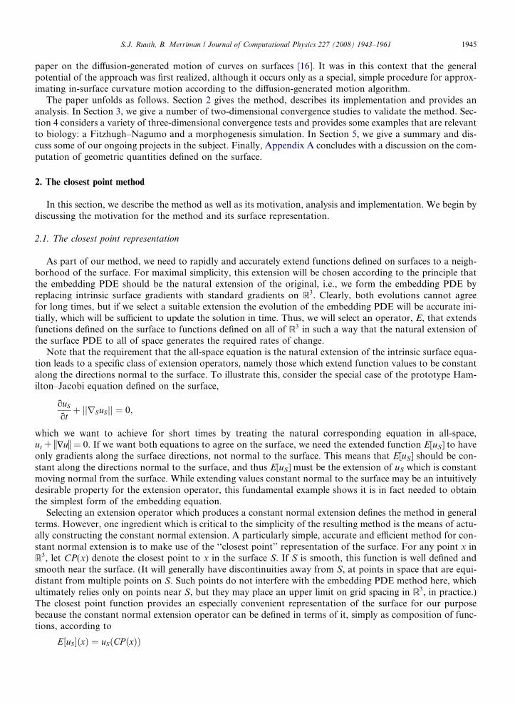
Consider first diffusion on the unit circle. Following [11], an initial profile

TableMax-n

Dx

0.20.10.050.0250.01250.0062

uSðh; 0Þ ¼ sinðhÞ

is assigned, which implies that the solution at any time t is given by

uSðh; tÞ ¼ expð�tÞ sinðhÞ:

We apply the closest point method to the problem using an analytical representation of the closest point func-tion. Time-stepping is carried out using forward Euler with a time step-size Dt = 0.1Dx2 and all interpolationsare accomplished with degree-four interpolation polynomials.

The relative errors in the result at the final time t = 1 were computed on the circle using the max-norm for avariety of Dx-values. These results are reported in Table 1.

As expected from the order of the spatial discretization, these results give a second-order error in the valueof u. We remark that the errors and convergence rates represent an improvement over those reported for arecent embedding method when computing on a band that adapts to the mesh size. See [11] for the resultsusing that level-set based method.

3.2. Advection equation

Our second test evolves a smooth initial profile on the ellipse

x2

a2þ y2

b2¼ 1; a ¼ 0:75; b ¼ 1:25 ð2Þ

according to the advection equation,

ouS

otþ ouS

os¼ 0;

where s is the arclength along the curve.

1orm relative errors for the heat equation on a circle

Error Conv. rate

1.03e�022.51e�03 2.046.26e�04 2.001.54e�04 2.023.84e�05 2.00

5 9.63e�06 2.00


The embedding partial differential equation is

TableMax-n

Dx

0.20.10.050.0250.01250.0062

ouotþ T ðx; yÞ � ru ¼ 0;

where the velocity

T ðx; yÞ ¼ V ðCP ðx; yÞÞ ð3Þ
is an extension of the value defined on the ellipse itself
V ððx; yÞÞ �ð� y

b2 ;x

a2Þffiffiffiffiffiffiffiffiffiffiffiffiy2

b4 þ x2

a4

q :

The closest point representation of the ellipse is precomputed on the underlying grid (to double precision)using Newton’s method applied to the derivative of the square of the distance function.

We consider the initial profile

uSðs; 0Þ ¼ cos2ð2ps=LÞ;
where s is arclength and L � 6.38174971583483 is the perimeter of the ellipse (cf. [11]). Our computations mea-sure the max-norm of the difference between our computed solution and the exact solution,
uSðs; tÞ ¼ cos2ð2pðs� tÞ=LÞ
for several different grid spacings to estimate the convergence rate.
Because second-order central differences are used, we must use a time-stepping scheme that includes theimaginary axis near the origin to achieve linear stability. For this reason, we use the popular third-orderTVD Runge–Kutta scheme [23,22]. In all calculations, the time step-size is set according to Dt = 0.5Dx andwe use third-order interpolation polynomials to carry out interpolations. Note that simple second-order cen-tral differences are effective for this smooth problem. If upwinding is required for the embedding PDE, how-ever, it may make sense to also use an interpolation step which is nonsymmetric. An example of such aninterpolation appears in [14], where a WENO-based interpolation procedure and standard WENO methodsfor Hamilton–Jacobi PDEs are used to solve level set equations on surfaces.

The relative errors at time t = 1 for a number of experiments are reported in Table 2, below.These results clearly demonstrate second-order convergence in the value of u. Thus, both the closest point

method and the recent level-set method of Greer [11] give second-order convergence when the bandwidth isadapted to the mesh-size. A direct comparison of the errors cannot be made in this example since we havetreated an ellipse rather than a circle.

3.3. Advection–diffusion equation

We conclude our examples in R2 with the evolution of a smooth initial profile on the ellipse (2) according tothe advection–diffusion equation,

ouS

otþ ouS

os¼ o2uS

os2;

where s is the arclength along the curve.

2orm relative errors for the advection equation on an ellipse

Error Conv. rate

3.88e�026.89e�03 2.491.72e�04 2.004.30e�04 2.001.07e�04 2.00

5 2.68e�05 2.00


The embedding partial differential equation is

TableMax-n

Dx

0.10.050.0250.01250.00620.00310.0015

ouotþ T ðx; yÞ � ru ¼ r2u

with velocity T(x, y) as defined in (3). In this example, we consider the initial profile

uSðs; 0Þ ¼ sin2ð2ps=LÞ;
where s is arclength and L is the perimeter of the ellipse (cf. [11]). Our computations measure the max-norm ofthe difference between our computed solution and the exact solution,
uSðs; tÞ ¼ expð�4tÞ sin2ð4pðs� tÞ=LÞ

for several different grid spacings to estimate the convergence rate. To ensure stability, time-stepping is carriedout using forward Euler with a time step-size Dt = 0.1Dx2. All interpolations are carried out using degree-fourpolynomials.

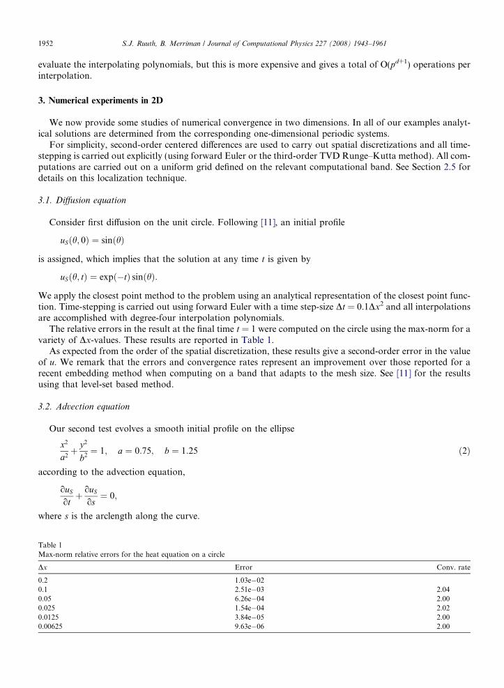
The relative errors arising at time t = 1 for a number of experiments are reported in Table 3.This convergence test also indicates a second-order convergence in the value of u. Similar to the case of

diffusion, the convergence rates represent an improvement over those reported for a recent level-set basedmethod [11] when computing on a band that adapts to the mesh size.

4. Numerical experiments in 3D

We now examine the numerical behavior of the method in three dimensions. Where analytical solutionsexist, numerical convergence studies are carried out.

Similar to the previous section, second-order centered differences are used to carry out spatial discretiza-tions and all time-stepping is carried out explicitly (using forward Euler or the third-order TVD Runge–Kuttamethod). All computations are carried out on a band around the surface.

4.1. Diffusion equation

Consider diffusion on the unit sphere. Following [11], we assign initial conditions

uSðh; g; 0Þ ¼ cosðgÞ

in spherical coordinates (r, h, g). As pointed out in [11], the corresponding initial value problem has exactsolution

uSðh; g; tÞ ¼ expð�2tÞ cosðgÞ:
The evolution is carried out using an analytical representation for the closest point function. Time-stepping
is carried out using forward Euler with a time step-size Dt = 0.1Dx2 and degree-four polynomials are used tocarry out interpolations. Calculating the max-norm relative error of the numerical result at the final time t = 1for several Dx-values gives the results reported in Table 4.

3orm relative errors for the advection–diffusion equation on an ellipse

Error Conv. rate

4.72e�023.85e�03 3.621.09e�03 1.822.96e�04 1.88

5 7.48e�05 1.9825 1.88e�05 2.00625 4.69e�06 2.00

Table 4Max-norm relative errors for the heat equation on a sphere

Dx Error Conv. rate

0.2 7.49e�030.1 2.14e�03 1.810.05 5.19e�04 2.050.025 1.30e�04 2.000.0125 4.38e�05 2.00


This convergence test also indicates a second-order convergence in the value of u. Similar to the two-dimen-sional case, the errors and convergence rates represent an improvement over those reported for a recent level-set based method applied to a band that adapts to the mesh size [11].

4.2. Advection equation

To study the numerical convergence for advection on a surface, we consider the example provided in [11].Specifically, we evolve on a torus defined by

TableMax-n

Dx

0.10.050.0250.01250.0062

1

2cosðgÞ þ 1

� �cosðhÞ; 1

2cosðgÞ þ 1

� �sinðhÞ; 1

2sinðgÞ

� �; �p 6 h; g < p

according to the advection equation ouSot þ

ouSog ¼ 0: The initial conditions are set equal to

uSðh; g; 0Þ ¼ f ðgÞ;

where f is the smooth function of period 2p defined by

f ðgÞ ¼gðgþp

p Þ �p 6 g 6 0

gðg�pp Þ 0 < g < p

(with gðxÞ ¼

expð 1x�1Þ � expð� 1

xÞexpð� 1

xÞ þ expð 1x�1Þ :

Computing using second-order centered differences, the third-order TVD Runge–Kutta scheme and degree-three interpolation polynomials with a time step-size Dt = 0.5Dx and varying Dx gives us a sequence of solu-tions. The corresponding max-norm relative errors at time t = 1 are reported in Table 5.

This convergence test also indicates a second-order convergence in the value of u. Thus, both the closestpoint method and the recent level set method of Greer [11] give second-order when the bandwidth is adaptedto the mesh-size. The errors generated by both methods for a particular mesh size are also very similar.

4.3. Curvature motion

Consider next the motion of a circular interface on a sphere evolving according to in-surface curvaturemotion. By symmetry, the interface remains a circle as it collapses. Moreover, it is straightforward to deter-mine the state of the system at any time t since the radius of the collapsing circle is governed by an ODE sys-tem which can be solved to high precision with standard ODE methods.

5orm relative errors for the advection equation on a torus

Error Conv. rate

3.82e�021.00e�02 1.932.44e�03 2.046.57e�04 1.89

5 1.62e�04 2.02


We represent the evolving contour by the zero level of the function / which is initially set equal toð2=3Þ �

ffiffiffiffiffiffiffiffiffiffiffiffiffiffiy2 þ z2

p. To achieve curvature motion, we wish to evolve / according to the embedding of the sur-

face PDE,

TableMax-n

Dx

0.050.0250.01250.0062

o/S

ot� rS �

rS/S

jjrS/Sjj

� �jjrS/S jj ¼ 0:

In our formulation, we therefore proceed simply by evolving the three-dimensional level-set equation,

o/ot� r � r/

jjr/jj

� �jjr/jj ¼ 0:

where j ¼ ðr � r/jjr/jjÞ is the mean curvature of the local level-set in R3. Similar to our other examples, the re-

quired initial conditions are obtained by extending the initial conditions on to the computational band usingthe closest point extension.

We select the sphere radius to be 1 and the initial radius of the circle to be 2/3. To discretize in time, forwardEuler is used with a time discretization parameter Dt = 0.1Dx2. Degree-four polynomials are used to carry outall interpolations. Convergence is studied by comparing the numerical radius at time t = 0.1 against the exactresult (0.56695935668549) for various Dt. The relative errors in the final radius from a number of experimentsare reported in Table 6.

This convergence test indicates a second-order convergence in the value of the circle radius.

4.4. Diffusion on a filament

Our final convergence test considers diffusion of a smooth initial profile on a helical curve

ðx; y; zÞ ¼ ðsinð2psÞ; cosð2psÞ; 2s� 1Þ ð4Þ
where 0 6 s 6 1 and homogeneous Neumann and Dirichlet conditions are imposed at the endpoints s = 0 ands = 1, respectively. Note this example involves a codimensional-two object with boundaries, so it is much morenaturally treated using a closest point representation than a level-set representation. The closest point repre-sentation of the helix is precomputed on the underlying grid (to double precision) using Newton’s method ap-plied to the derivative of the square of the distance function.
To examine the numerical convergence, we consider the initial profile

uSðs; 0Þ ¼ cosð0:5psÞ:
Our computations measure the max-norm of the difference between our computed solution and the exactsolution,
uSðs; tÞ ¼ exp � p2L

� �2

t� �

cosð0:5psÞ

where L ¼ffiffiffiffiffiffiffiffiffiffiffiffiffi1þ p2p

is the length of the helix.No special treatment is required at the homogeneous Neumann boundary since the value at that endpoint is

naturally extended throughout space at each step using the closest point function. At the homogeneous Dirich-let condition the treatment is also straightforward: instead of propagating out the numerical value at that end-point, we propagate out the prescribed boundary value (in this case uS(1, t) = 0).

6orm relative errors for curvature motion on the sphere

Error Conv. rate

3.35e�048.22e�05 2.032.05e�05 2.01

5 5.11e�06 2.00

Table 7Max-norm relative errors for diffusion on a helix with boundary conditions

Dx Error Conv. rate

0.2 1.53e�020.1 7.64e�03 1.010.05 3.82e�03 1.000.025 1.91e�03 1.000.0125 9.54e�04 1.00


Time stepping is carried out to time t = 1 using forward Euler with Dt = 0.1Dx2. Evaluating the max-normrelative errors for several different grid spacings gives the numerical convergence rate results presented inTable 7. Our interpolations are carried out using degree-three polynomials since higher orders did not signif-icantly influence the errors.

As we can see from the table, the introduction of simple boundary conditions gives a consistent calcu-lation, however, the result is only first-order accurate. When boundary conditions are enforced in thismanner, the extended function is continuous but certain derivatives may be discontinuous near the bound-aries. (In this example, discontinuities in the first derivatives occur on a planar region which is orthogonalto the filament at the Dirichlet boundary, s = 1. Discontinuities in the second derivatives occur on a pla-nar region which is orthogonal to the filament at the homogeneous Neumann boundary, s = 0.) This lossof regularity contributes to a loss of accuracy in the interpolation procedure and the discretization of theembedding PDE.

The development of methods that gives an improved treatment of boundary conditions is of strong interestto us and is a part of our ongoing investigations.

4.5. Reaction diffusion systems

We conclude our numerical experiments by providing some applications to reaction diffusion systems.Fig. 3 gives an example of a spiral wave evolving on a sphere, as computed by our approach. The simulated

system in this example is the well-known Fitzhugh–Nagumo equations [9]

ouS

ot¼ ða� uSÞðuS � 1ÞuS � vS þ mr2

SuS ; ð5Þ

ovS

ot¼ �ðbuS � vSÞ; ð6Þ

where uS is the excitation variable, � = 0.01, a = 0.1, b = 0.5 and m = 0.0001. To obtain an attractive spiralwave, we set our initial conditions according to

ðuS ; vSÞ ¼ð1; 0Þ if x > 0; y > 0; z > 0;

ð0; 1Þ if x < 0; y > 0; z > 0;

ð0; 0Þ otherwise:

8><>:

This simulation set Dt = 0.0390625 and Dx = 0.00625. Doubling these discretization step sizes gave very sim-ilar results.

Fig. 4 gives an example of a Turing pattern formation model [26] evolving on the surface of a U-shapedtube, as computed by our approach. The simulated system in this example is the Schnakenberg system [21],

ouS

ot¼ cða� uS þ u2

SvSÞ þ r2SuS ; ð7Þ

ovS

ot¼ cðb� u2

SvSÞ þ mr2SvS ; ð8Þ

where uS is the activator and vS is the inhibitor. To perturb the system away from equilibrium, we set the initialconditions at each point (x, y, z) on the surface according to

Fig. 3. Fitzhugh–Nagumo equation evolving on a sphere. The excitation variable u is displayed at times t = 375, 437.5, 500 and 562.5.This simulation takes Dt = 0.0390625, D x = 0.00625 and uses an analytical representation of the closest point to the sphere. ForwardEuler time-stepping and degree-four interpolating polynomials are used throughout the calculation.

Fig. 4. Schnakenberg system evolving on a U-shaped tube. The activator u is displayed at times t = 0.01, 0.03, 0.05, 0.13. This simulationtakes Dt = 1.5625e�07, Dx = 1/160 and uses an analytical representation of the closest point to the tube. Forward Euler time-stepping anddegree-three interpolating polynomials are used throughout the calculation.


uSðx; y; zÞ ¼ aþ bþX5

i¼1

1

20isinð2pixÞ sinð2piyÞ sinð2pizÞ;

vSðx; y; zÞ ¼a

ðaþ bÞ2þX5

i¼1

1

20icosð2pixÞ cosð2piyÞ cosð2pizÞ:

In this calculation steady patterns are sought, so the free parameters are set according to some values appear-ing in [19]: c = 500, a = �.048113, b = 1.202813 and m = 120. This simulation took Dt = 1.5625e�07 andDx = 1/160, and we note that doubling these discretization step sizes produced similar results. Because thisproblem is numerically stiff, implicit time-stepping would be highly desirable. A focus of our current workis the design of efficient methods for treating implicit time-discretizations using the closest point method.


5. Summary and future work

In this work, we present the closest point method, which is a new embedding method for solving partialdifferential equations on surfaces. The method is designed to make solving PDEs on surfaces as close aspossible to the familiar process of solving PDEs in R3, in effect hiding all the geometric complexities. Cen-tral to the method is the choice of the closest point representation of the surface. This representation nat-urally gives an extension step which leads to embedding PDEs that are simply the surface PDEs withsurface gradients replaced by standard gradients in R3. This representation also gives the flexibility to treatopen surfaces, surfaces without orientations, objects of codimension-two or higher or collections of objectswith varying codimension. We further remark that it is straightforward to compute on a narrow bandaround the surface using the closest point method and that (unlike other embedding methods) bandingcan be carried out without any degradation in the accuracy of the underlying discretization. The net resultis that the method is remarkably simple: instead of treating a surface PDE it treats the corresponding PDEin the embedding space using standard numerical methods on uniform Cartesian grids. This means thatexisting software for three-dimensional flows can be modified to carry out surface flows with the minimalprogramming effort.

A variety of numerical experiments were carried out to validate the method. It was found that the numericalconvergence rates agreed with the convergence rates of the underlying spatial discretizations. The errors pro-duced by the method for a given mesh width were similar or better than those reported for a recent embeddingmethod [11].

There are many opportunities for further development of the closest point method. In particular, we areinvestigating the use of ENO and WENO based interpolation to give methods suitable for nonsmooth flows(e.g. [14]). The generalization of the method to implicit time-stepping and elliptic equations on surfaces is alsoof strong interest to us, since many flows are too stiff to be conveniently treated by explicit methods (e.g. [12]).Formally, the analysis developed in Section 2.3 still applies to such equations, however, the solution of thecorresponding nonlinear equations will be complicated by the closest point operator. Another area of researchinterest is the improved treatment of boundary conditions for open surfaces. In this paper, first-order accuracywas obtained using a straightforward extension of boundary data but we anticipate more sophisticated meth-ods should yield more accurate results.

The study of more general flows or flows on more general objects is also of interest. For example, the treat-ment of third- and higher-order PDEs should be further investigated. While such applications can be solvedusing multiple applications of the closest point mapping, we have not yet investigated this class of problemsnumerically. Other potential targets for future work include solving PDEs on surfaces with edges/corners, oreven point clouds of data, as the general closest point method formalism still applies even when the underlyingnotion of a PDE on the object is no longer clearly defined.

While this paper focuses on the important case of static surfaces, the treatment of moving surfaces alsoappears in applications (e.g., [29]) and is another interesting topic for investigation. In such applications, itis important to note an advantage that level-set representations have over closest point representations:level-set representations of surfaces can be evolved using well-known and robust discretizations of thelevel-set equation, whereas the evolution of closest point representations is less well understood (cf.[24,20]). This advantage is particularly pronounced in flows involving surfaces that merge or break apart, sincelevel-set methods treat such problems naturally and automatically.

Finally, we conclude by noting that the closest point method’s simplicity and flexibility make it an excellentcandidate for treating areas of application in the natural and applied sciences. See [27,28,7,8,17,18] and thereferences in [3,11] for a sample of some application areas that treat PDEs on surfaces.

Appendix A. Calculation of surface normal and curvature

The surface normal and curvature are fundamental geometric properties of the surface, and are of interestfor a variety of purposes. In the context of solving surface PDEs, our main concern is that such quantitiescould occur explicitly within the PDE, for example, in the form of a curvature-dependent reaction rate in areaction diffusion equation.


If these geometric quantities are available as a given function on the surface, our general formalism wouldimmediately apply. However, it is more likely that they will actually need to be computed from the surfaceitself, prior to any extension. Thus, we provide a convenient way to compute these quantities directly fromthe closest point representation of the surface, CP(x).

First, consider constructing a normal vector field, N. In terms of the closest point function, this is quitesimple. Given any point x in R3, the vector x � CP(x) extends from the surface at CP(x) to the point x, ina direction normal to the surface. Thus, normalizing this vector field

NðxÞ ¼ x� CP ðxÞjjx� CP ðxÞjj

provides a suitable extension of the normal where the direction points away from the surface. In some applica-tions, the fact that the vector field N changes direction discontinuously at the surface may preclude the imme-diate use of this formula. For example, the discontinuity at the surface is undesirable in the curvature formulasbelow. For such situations, we need to make a choice of one of the two available directions at the surface asthe preferred direction, and reverse the direction of N on the other side. This choice can be encapsulated in asign function s(x) defined near the surface that is +1 on one side of surface, and �1 on the other. This is ineffect a choice of ‘‘outward normal direction’’, or orientation, for the surface, which is always needed to definethe overall sign of the curvature, independent from the issues at hand. Given such a sign function, then thevector field

nðxÞ ¼ sðxÞNðxÞ ð9Þ

is a suitable extension of a unit normal field on the surface to all of space. Note this is not strictly defined at thesurface, since N(x) is not defined there. At such points, however, N(x) can be assigned its limiting value,approaching from off the surface.

The sign function s(x) must somehow be constructed independently, as it is not determined by the surfaceitself, or the closest point function. For example, if the surface is closed, with a well-defined inside region, theindicator function of this inner region can be used to define s. Or, if a signed distance function is available, thesign from that can be adopted for s.

For general curvature flows we may compute curvature from an extension of the unit normal vector field.Specifically, let n be a unit vector field defined on R3 that reduces to a unit normal vector field along the sur-face. Then the mean curvature of the surface, j, is given by the divergence of this vector field

j ¼ r � n
at the surface, and this relation provides a convenient embedding of the mean curvature off the surface as well.More generally, all properties of the curvature can be obtained from the curvature matrix K, which can becomputed as the total derivative of the normal vector field
K ¼ rn

at the surface, and similarly using this formula to extend K off the surface. The matrix K has n itself as a trivialeigenvector, with eigenvalue 0, reflecting the constant length of n. The nontrivial eigenvectors of this matrixare tangent to the surface and define the directions of principal (maximal and minimal) curvature, and thecorresponding eigenvalues j1 and j2 are the principal curvatures at the point in question. The mean curvatureis the sum of these principal curvatures, or, equivalently, the trace of the matrix K, which yields the divergenceformula given previously.

Alternatively, certain curvature-dependent quantities can be obtained from the closest point function itself.For example, it is easily shown [20] that at the surface the vector mean curvature is given by the Laplacian ofthe closest point function, i.e.,

�jn ¼ r2CP

for any point on the surface S. This vector-valued quantity corresponds to the velocity of the surface undergradient descent on the surface area, or equivalently, it is the first variational derivative of the surface area,and thus is a quantity of particular importance. From this, the mean curvature can be determined by


j ¼ � r2CP� �

� n;

where n is a given choice of the unit normal.

References

[1] M. Berger, Finite Element Approximation of Elliptic Partial Differential Equations on Implicit Surfaces, CAM Report 05-46,University of California, Los Angeles, 2005.

[2] J.-P. Berrut, L.N. Trefethen, Barycentric Lagrange interpolation, SIAM Review 46 (3) (2004) 501–517.[3] M. Bertalmıo, L.T. Cheng, S. Osher, G. Sapiro, Variational problems and partial differential equations on implicit surfaces, Journal

of Computational Physics 174 (2001) 759–780.[4] M. Bertalmıo, F. Memoli, L.T. Cheng, G. Sapiro, S. Osher, Variational problems and partial differential equations on implicit

surfaces: bye bye triangulated surfaces? in: S. Osher, N. Paragios (Eds.), Geometric Level Set Methods in Imaging, Vision, andGraphics, Springer, New York, 2003, pp. 381–398.

[5] Richard L. Burden, J. Douglas Faires, Numerical Analysis, seventh ed., Brooks/Cole, 2001.[6] L.-T. Cheng, P. Burchard, B. Merriman, S. Osher, Motion of curves constrained on surfaces using a level-set approach, J. Comput.

Phys. 175 (2) (2002) 602–644.[7] U. Diewald, T. Preufer, M. Rumpf, Anisotropic diffusion in vector field visualization on Euclidean domains and surfaces, IEEE Tran.

Vis. Comput Graph. 6 (2000) 139–149.[8] J. Dorsey, P. Hanrahan, Digital materials and virtual weathering, Sci. Am. 282 (2) (2000) 282–289.[9] R. FitzHugh, Fitzhugh–Nagumo simplified cardiac action potential model, Biophys. J. 1 (1961) 445–466.

[10] M.S. Floater, K. Hormann, Surface parameterization: a tutorial and survey, in: N.A. Dodgson, M.S. Floater, M.A. Sabin (Eds.),Advances in Multiresolution for Geometric Modelling, Heidelberg, 2005, pp. 157–186.

[11] J.B. Greer, An improvement of a recent Eulerian method for solving PDEs on general geometries, J. Sci. Comput. 29 (3) (2006) 321–352.

[12] J.B. Greer, A.L. Bertozzi, G. Sapiro, Fourth order partial differential equations on general geometries, J. Comput. Phys. 216 (1)(2006) 216–246.

[13] G.-S. Jiang, C.-W. Shu, Efficient implementation of weighted ENO schemes, J. Comput. Phys. 126 (1996) 202–228.[14] C.B. Macdonald, S.J. Ruuth, Level set equations on surfaces via the closest point method, submitted for publication.[15] S. Mauch, Efficient Algorithms for Solving Static Hamilton Jacobi Equations, PhD Thesis, California Institute of Technology,

Pasedena, 2003.[16] B. Merriman, S.J. Ruuth, Diffusion generated motion of curves on surfaces, J. Comput. Phys. 225 (2) (2007) 2267–2282.[17] T.G. Myers, J.P.F. Charpin, A mathematical model for atmospheric ice accretion and water flow on a cold surface, Int. J. Heat Mass

Transf. 47 (25) (2004) 5483–5500.[18] T.G. Myers, J.P.F. Charpin, S.J. Chapman, The flow and solidification of a thin fluid film on an arbitrary three-dimensional surface,

Phys. Fluids 14 (8) (2002) 2788–2803.[19] S.J. Ruuth, Implicit–explicit methods for reaction–diffusion problems in pattern-formation, J. Math. Biol. 34 (2) (1995) 148–176.[20] S.J. Ruuth, B. Merriman, S. Osher, A fixed grid method for capturing the motion of self-intersecting interfaces and related PDEs, J.

Comput. Phys. 163 (2000) 1–21.[21] J. Schnakenberg, Simple chemical-reaction systems with limit-cycle behavior, J. Theor. Biol. 81 (3) (1979) 389–400.[22] Chi-Wang. Shu, Total-variation-diminishing time discretizations, SIAM J. Sci. Statist. Comput. 9 (6) (1988) 1073–1084.[23] Chi-Wang. Shu, Stanley. Osher, Efficient implementation of essentially nonoscillatory shock-capturing schemes, J. Comput. Phys. 77

(2) (1988) 439–471.[24] J. Steinhoff, M. Fan, L. Wang, A new Eulerian method for the computation of propagating short acoustic and electromagnetic pulses,

J. Comput. Phys. 157 (2) (2000) 683–706.[25] J. Strain, Fast tree-based redistancing for level set computations, J. Comput. Phys. 152 (1999) 648–666.[26] A.M. Turing, The chemical basis of morphogenesis, Roy. Soc. Lond. Philos. Trans. Ser. B 237 (1952) 37–72.[27] G. Turk, Generating textures on arbitrary surfaces using reaction–diffusion, Comput. Graph. 25 (4) (1991) 289–298.[28] A. Witkin, M. Kass, Reaction–diffusion textures, Comput. Graph. 25 (4) (1991) 299–308.[29] J. Xu, H.-K. Zhao, An Eulerian formulation for solving partial differential equations along a moving interface, J. Sci. Comput. 19 (1–

3) (2003) 573–594.

Documents

A simple embedding method for solving partial differential equations on surfaces