A Simple Approach to Overcome the Problems

From the Keynesian Stability Condition:

Extended Version

Reiner Franke∗

University of Kiel (GER)

December 2015

Abstract

The Keynesian stability condition is a necessary assumption for the IS equi-

librium concept to make economic sense. With reasonable values for the sav-

ing parameter(s), however, it typically implies excessively strong multiplier

effects. This is more than a cosmetic issue, not the least because any simula-

tion study of an otherwise ambitious model will thus be fraught with severe

problems along some of its dimensions. The present paper demonstrates that

by introducing proportional tax rates on production, corporate income and

personal income, the multipliers will be considerably dampened. Within an

elementary Kaleckian framework, the paper furthermore advances a fairly sat-

isfactory numerical calibration, which also takes some ratios around the gov-

ernment deficit into account. Lastly, a stylized cyclical scenario explores the

amplitudes and comovements of the oscillating dynamic variables.

JEL classification: C 02, D84, E12, E30.

Keywords: Investment multiplier, proportional taxes, public debt, functional

finance, moment matching.

1 Introduction

It is a convenient practice in post-Keynesian structuralist modelling to employ the

device of continuous goods market clearing. For the instantaneous output adjust-

ments and their implications to make economic sense, it is then necessary to assume

∗Email: franke@uni-bremen.de .

1

that the sensitivity of investment to changes in utilization is lower than the utiliza-

tion sensitivity of aggregate saving. This requirement is usually referred to as the

Keynesian stability condition.

Although the condition is universally applied, it is not without problems.

With ordinary saving functions it is well-known that reasonable values of their pa-

rameter(s) cause excessively strong reactions of IS utilization to changes in the

variables of the model or some of the parameters. This feature could be perhaps

neglected as long as the models remain relatively simple and one is only interested

in the sign of the reactions. However, when the models become more complex and

so numerical simulations can no longer be avoided, the strong multiplier effects are

rather awkward and can also easily give rise to misleading conclusions.

In this situation most of the literature simply chooses to accept the dispro-

portions among some of the model’s variables, apparently hoping that the essential

properties of the model do not suffer too much from them. Alternatively, one way

out is the specification of a more elaborated saving behaviour with dynamic ele-

ments.1 While this is important work to introduce a more realistic flavour, it has the

disadvantage that it loses contact with the elementary modelling of the profession

and the economic wisdom established there. The present contribution therefore pro-

poses a less radical way. It starts out from a canonical Kaleckian macro model, for

concreteness, and augments it by a government sector where, in particular, it ad-

vances proportional tax rates on different income sources. The central point of this

approach is that the corresponding modifications of aggregate demand will weaken

the original reactions of the IS utilization rate. This finding leads us then to a nu-

merical issue, namely, whether the dampening of the multiplier effects could also

be quantitatively significant.

Besides, sooner or later the baseline models need to take government activ-

ities into account, even if they follow rigid rules, and then taxes will have to be

introduced anyway.

The paper is organized as follows. Section 2 starts out from the canonical

Kaleckian model and recapitulates the problems that the Keynesian stability condi-

tion poses at various methodological levels. Section 3 introduces the government

sector with its expenditures on the one hand, and the tax collections from produc-

tion, corporate income and personal income, on the other hand. It is then easily

seen that the income effects of the latter alleviate the IS equilibrium reactions.

1Some references will be given in Section 2 below. Still a different direction was chosen in a

number of papers and books by the so-called ‘Bielefeld School’ (e.g., Chiarella et al., 2005; the

expression itself was coined by J. Barkley Rosser, see p. xv). This approach abandons IS altogether,

which for consistency requires the introduction of inventories and thus a rule for inventory invest-

ment (with Metzler as its patron saint). A problem with this treatment, then, is that the inventory

accelerator can interfere with other dynamic effects that may be felt to be more important.

2

As the government budget will generally not be balanced, our extension im-

plies changes in the bonds that the government issues to finance its deficit. The fi-

nancing of private investment is also included in the model, though in a most simple

way. Section 4 makes these dynamic elements explicit and studies the steady state

positions that are constituted by the synchronous growth of the capital stock and

the stocks of public and private debt. Against this background, Section 5 turns to a

quantitative assessment of the IS multiplier effects. On the basis of some empirical

key rates and ratios, it investigates how close the model can come to the empirical

tax-to-GDP ratio and a proxy for the investment multiplier. Subsequently, Section

6 discusses possible improvements upon such an attempt at a calibration. Section 7

sets up stylized oscillations of the model’s exogenous variables at a business cycle

frequency and studies the resulting cyclical properties of the endogenous variables,

which are also contrasted with typical numerical examples from the literature. Sec-

tion 8 concludes. Some details regarding mathematics and data issues are relegated

to an appendix.

2 The Keynesian stability condition and its problems

in the short and long period

To set the stage, consider the canonical Kaleckian growth model (Lavoie, 2014,

Section 6.2.1) of a closed one-good economy without a public sector and without

financial constraints, where technical change is Harrod-neutral and labour is in per-

fectly elastic supply:

r = hu − δ (1)

gs = sr r (2)

gi = g⋆ + β (u−ud) (3)

gi = gs (4)

The first equation introduces the rate of profit, r. It is basically determined by the

product of the share of profits in total income, h, and the output-capital ratio u,

while the rate δ nets outs capital depreciation. The output-capital ratio will also be

referred to as (capital) utilization.

The function gs in (2) represents the aggregate saving in the economy, nor-

malized by the (replacement value of the) capital stock: workers consume all of

their wages, the profits of the firms are completely paid out to the shareholders, and

sr is the propensity to save out of this rentier income. The third equation specifies

the investment function, i.e. the planned growth rate of the capital stock, which is

3

based on a trend rate of growth g⋆ as it is currently perceived by the firms.2 The

second term in (3) refers to a “normal” or desired rate of utilization ud . This con-

cept admits of overutilization, when u > ud , and says that in such a situation the

firms seek to reduce this gap by increasing the capital stock at a higher rate than

g⋆; correspondingly for underutilization, when u < ud . For our present purpose it is

useful to treat the profit share h, the trend growth rate g⋆ and desired utilization ud

as exogenously fixed parameters.

Equation (4) postulates goods market equilibrium. The market clearing is

brought about by quantity variations, from which the rate of utilization results as

u =g⋆ + sr δ − βud

sr h − β(5)

With more elaborated investment functions than (3) some other dynamic variables

may additionally show up in the numerator, where we are especially thinking of the

ratios of financial assets to the capital stock. This notwithstanding, stability of the

quantity adjustment process requires the denominator of (5) to be positive, that is,

investment must be less sensitive to changes in utilization than saving:

β < sr h (6)

This is the well-known Keynesian stability condition. It also means that the multi-

plier works out in the correct direction: for example, ceteris paribus utilization will

rise when the firms expect a higher trend growth rate g⋆ and therefore increase their

investment demand. Besides, with (6) the much celebrated paradox of thrift ob-

tains according to which a higher saving propensity reduces rather than stimulates

economic activity.

The Keynesian stability condition might be accepted if eqs (1) – (4) are re-

garded as a description for the short period. Following Skott’s (2012, p. 134) argu-

ment in a discrete-time setting, the investment function includes several lags and in

the short period these effects can be thought of as being part of a constant term like

g⋆. The remaining reactions to the contemporaneous utilization rate could thus be

rather weak.

A more serious issue is the assumption in the Kaleckian approach that the

short-run condition applies in the long run as well. Hence there would be no real

loss in using a static specification of the investment function, as in eq. (3), for this

time frame. The elimination of lags and explicit dynamics only serves to simplify

the analysis and to provide a convenient platform for extensions in various direc-

tions (cf. Skott, 2012, p. 134). In this case it has, however, to be taken into account

that the coefficient β sums up the reactions to all of the lagged utilization rates. As

2Such a term is also often dubbed the firms’ ‘animal spirits’.

4

a consequence, it is then no longer obvious that such a modified coefficient β will

still be less than srh. Skott (2012) develops this argument in greater detail (with

a slightly different saving function) and concludes that even an a priori reasoning

and a sketchy empirical analysis fail to produce any evidence for a sufficiently weak

responsiveness of investment to utilization. Similar assessments can also be found

elsewhere in the literature (Dallery, 2007, Section IV, or Lavoie, 2010, p. 136).

Postulating multiple lags in a functional relationship is a straightforward econ-

ometric approach to filter out from the data the reactions of the firms in a changing

environment. It can thus give some hints to the specification of dynamic adjust-

ments in a small-scale model, but as a stylized behavioural description of the firms’

investment it is less convincing. The short period can, however, be readily and con-

sistently linked to the long period, and high values of β maintained in the investment

function, if gi in (3) is regarded as an investment rule that the firms would follow

under stable circumstances. In the presence of short-run fluctuations, on the other

hand, current investment will generally deviate from this level. The point is that the

firms perceive this as a disequilibrium situation and that they, realistically, seek to

close the gap between their current and desired investment not instantaneously but

in a gradual procedure.

Accordingly, treat the capital growth rate g as a variables that is predeter-

mined within the short period and suppose sluggish adjustments of g towards gi.

Substituting (1) in (2) and writing the saving function as gs = gs(u), the temporary

IS equilibrium condition reads g = gs(u) and utilization is given as a function of the

current capital growth rate,

u = u(g) =g + sr δ

sr h(7)

The capital growth rate is a dynamic variable that changes over time. With an

adjustment speed λ > 0 and working in continuous time, its motions are governed

by the adjustment equation

g = λ {gi[u(g)] − g} (8)

where for the sake of the argument the trend growth rate g⋆ in the investment func-

tion (3) continues to be fixed.3 Incidentally, a dynamic model like (7), (8) may be

viewed as a Kaleckian model of an earlier generation. Rather than the level of in-

vestment, it considers it more appropriate to specify the change in investment as the

relevant endogenous variable. In fact, this idea is often attributed to Steindl (1952).

The nowadays common alternative that makes g (not g) a function of utilization

3An assumption that g⋆ directly or indirectly increases when utilization u increases would intro-

duce a Harrodian, i.e. destabilizing mechanism.

5

(and perhaps other variables) can be said to have started later with, in particular, the

contributions by Rowthorn (1981), Dutt (1984), Bhaduri and Marglin (1990).

By construction, the Keynesian stability condition poses no problem for the

short-run utilization in eq. (7). The condition nevertheless raises its head when it

comes to the stability of the long-run dynamics. Equation (8) constitutes a one-

dimensional differential equation (8) in g, and it is easily checked that its derivative

with respect to g is negative and therefore stability prevails if, and only if, inequality

(6) holds true again.

There seems to be a tendency to believe that stability is required for a model

to be economically meaningful, and for its steady state to be empirically relevant.

However, in general this is an unnecessarily strong point of view.4 For one thing,

global divergence can be avoided if one or two suitable nonlinearities are intro-

duced into the model. Second and equally importantly, an unstable steady state

growth path does not need to lose its explanatory power as it is consistent with en-

dogenously generated, bounded fluctuations around it. That is, the steady state is

locally repelling, as in the original setting, while some stabilizing forces become

dominant in the outer regions of the state space. The steady state solution may then

still provide a good approximation of the medium-run time averages of the global

dynamics.

Although these arguments may be accepted in general, they do not solve all

of the problems. To begin with, observe that also utilization in the steady state of

system (7), (8) is given by eq. (5).5 Hence a violation of the Keynesian stability

condition would imply that a higher trend growth rate g⋆ lowers the utilization rate

in the new steady state (where, in line with ‘Kaleckian’ theory as it is presently

often understood, actual and desired utilization may differ). By the same token,

the paradox of thrift would fail to apply. As these conclusions (or at least the first

one) do not appear acceptable, the dynamic version of the Kaleckian baseline model

would not get rid of the Keynesian stability condition, either.

Even if the Keynesian stability condition is approved, there is still a second

problem that often goes unnoticed. It will become more serious when the model

is extended and thus gets so complex that its analysis has to rely on numerical

simulations. To illustrate the problem, consider the steady state values that with

reference to the US economy will later be employed in our own numerical cali-

bration. These are a depreciation rate δ = 10%, a profit share h = 31%, a growth

rate g = 2.50%, and an output-capital ratio u = 0.90. The corresponding profit rate

is r = 17.9% and from eq. (2), g = srr, the saving propensity sr is residually de-

4The following reasoning joins Skott (2010, p. 115), to name just one explicit reference.5Utilization u would here coincide with desired utilization ud if (and only if) the trend growth

rate g⋆ in (3) satisfies g⋆ = sr(hud−δ ) as a consistency condition.

6

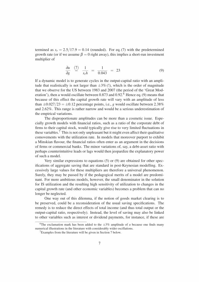
termined as sr = 2.5/17.9 = 0.14 (rounded). For eq. (7) with the predetermined

growth rate (or if we assume β = 0 right away), this implies a short-run investment

multiplier of

∂u

∂g

(7)=

1

srh=

1

0.043= 23 (9)

If a dynamic model is to generate cycles in the output-capital ratio with an ampli-

tude that realistically is not larger than ±3% (!), which is the order of magnitude

that we observe for the US between 1983 and 2007 (the period of the ‘Great Mod-

eration’), then u would oscillate between 0.873 and 0.92.6 Hence eq. (9) means that

because of this effect the capital growth rate will vary with an amplitude of less

than ±0.027/23 =±0.12 percentage points, i.e., g would oscillate between 2.38%

and 2.62%. This range is rather narrow and would be a serious underestimation of

the empirical variations.

The disproportionate amplitudes can be more than a cosmetic issue. Espe-

cially growth models with financial ratios, such as a ratio of the corporate debt of

firms to their capital stock, would typically give rise to very limited fluctuations in

these variables.7 This is not only unpleasant but it might even affect their qualitative

comovements with the utilization rate. In models that moreover purport to exhibit

a Minskian flavour, the financial ratios often enter as an argument in the decisions

of firms or commercial banks. The minor variations of, say, a debt-asset ratio with

perhaps counterintuitive leads or lags would then jeopardize the explanatory power

of such a model.

Very similar expressions to equations (5) or (9) are obtained for other spec-

ifications of aggregate saving that are standard in post-Keynesian modelling. Ex-

cessively large values for these multipliers are therefore a universal phenomenon.

Surely, they may be passed by if the pedagogical merits of a model are predomi-

nant. For more ambitious models, however, the small denominator in the solution

for IS utilization and the resulting high sensitivity of utilization to changes in the

capital growth rate (and other economic variables) becomes a problem that can no

longer be neglected.

One way out of this dilemma, if the notion of goods market clearing is to

be preserved, could be a reconsideration of the usual saving specifications. The

remedy is to reduce the direct effects of total income (and thus total output or the

output-capital ratio, respectively). Instead, the level of saving may also be linked

to other variables such as interest or dividend payments, for instance, if these are

6The exclamation mark has been added to the ±3% amplitude of u because one finds many

numerical illustrations in the literature with considerably wider oscillations.7Examples from the literature will be given in Section 7 below.

7

predetermined variables in a model. One stimulation in this direction could be the

saving function postulated by Hein and Schoder (2011) in their empirical investi-

gation (cf. their equations (10) and (13) on pp. 696f). Another and more involved

treatment referring to financial variables and dynamic adjustments can be found in

some papers by Skott and Ryoo (e.g., Skott, 1989, Section 4.10; Skott and Ryoo,

2008, Section 3.1.3; Ryoo and Skott, 2015, Section 2.2.3).

Our contribution proposes a less radical way and basically sticks to the con-

cepts underlying the above saving function (2). The only direction into which the

baseline model is extended is the introduction of government spending and, there-

fore, taxes as one of its financing sources. Obviously, the multiplier effects could

also be weakened by postulating a countercyclical fiscal policy, but our results

should not depend on this feature. The primary subject will be the modification

of the investment multiplier by taxes that in a more or less direct way change with

economic activity and so have an adverse effect on aggregate demand.

3 Introduction of a government sector

This section adds a government sector to the canonical Kaleckian model. Govern-

ment expenditures are financed by taxes and, if a gap still persists, by the issuance of

new bonds. Four types of taxes are considered: taxes on wages, on rentiers income,

on corporate income, and on production. All of them change proportionally with

the corresponding tax base. For simplicity, the households are supposed to be taxed

identically, with the tax rate τp on Personal income.8 The tax rate on Corporate

income is designated τc, and τv denotes the tax rate on the volume of production, or

(gross) Value added.

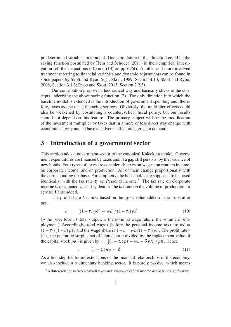
The profit share h is now based on the gross value added of the firms after

tax,

h = [(1− τv) pY − wL]/(1− τv) pY (10)

(p the price level, Y total output, w the nominal wage rate, L the volume of em-

ployment) Accordingly, total wages (before the personal income tax) are wL =(1− τv)(1−h) pY , and the wage share is 1−h = wL/(1− τv) pY . The profit rate r

(i.e., the operating surplus net of depreciation divided by the replacement value of

the capital stock pK) is given by r = [(1− τv) pY −wL−δ pK]/ pK. Hence

r = (1− τv)hu − δ (11)

As a first step for future extensions of the financial relationships in the economy,

we also include a rudimentary banking sector. It is purely passive, which means

8A differentiation between payroll taxes and taxation of capital income would be straightforward.

8

the banks accept deposits from the rentier households and give business loans to

the firms; the interest rates on deposits and loans are identical ( j); and banking

involves neither costs nor profits (neither households nor firms hold cash and the

amount of loans is equal to the amount of deposits). D being their stock of debt,

firms pay interest jD to the banks and these are directly transferred to the rentiers.

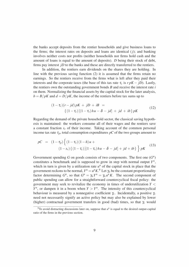
In addition, the rentiers earn dividends on the shares they are holding. In

line with the previous saving function (2) it is assumed that the firms retain no

earnings. So the rentiers receive from the firms what is left after they paid their

interests and the corporate taxes (the base of this tax rate τc is r pK− jD). Lastly,

the rentiers own the outstanding government bonds B and receive the interest rate i

on them. Normalizing the financial assets by the capital stock for the later analysis,

b = B/pK and d = D/pK, the income of the rentiers before tax sums up to

(1− τc)(r− jd) pK + jD + iB =

{(1− τc) [(1− τv)hu − δ − jd] + jd + ib} pK(12)

Regarding the demand of the private household sector, the classical saving hypoth-

esis is maintained: the workers consume all of their wages and the rentiers save

a constant fraction sr of their income. Taking account of the common personal

income tax rate τp, total consumption expenditures pC of the two groups amount to

pC = (1− τp){

(1− τv)(1−h)u +

(1− sr){(1− τc) [(1− τv)hu − δ − jd] + jd + ib}}

pK(13)

Government spending G on goods consists of two components. The first one (Gn)

constitutes a benchmark and is supposed to grow in step with normal output Y n,

which in turn is given by a utilization rate un of the capital stock in place that the

government reckons to be normal, Y n = unK.9 Let γn be the constant proportionality

factor determining Gn, so that Gn = γnY n = γn un K. The second component of

public spending can allow for a straightforward countercyclical fiscal policy: the

government may seek to revitalize the economy in times of underutilization Y <Y n, or dampen it in a boom when Y > Y n. The intensity of this countercyclical

behaviour is measured by a nonnegative coefficient γc. Incidentally, a positive γc

need not necessarily signify an active policy but may also be explained by lower

(higher) contractual government transfers in good (bad) times, so that γc would

9To avoid distracting discussions later on, suppose that un is equal to the desired output-capital

ratio of the firms in the previous section.

9

capture some elements of the ‘automatic stabilizers’. In sum, government spending

is given by G = γnY n − γc (Y −Y n), or

G = [γn un − γc (u−un) ] K (14)

The remaining two components of aggregate demand are replacement investment

δ K and net investment gK. To ease the discussion, the capital growth rate will from

now on be treated as a predetermined variable. That is, the investigation will focus

on the size of the multiplier effects from exogenous variations of net investment.

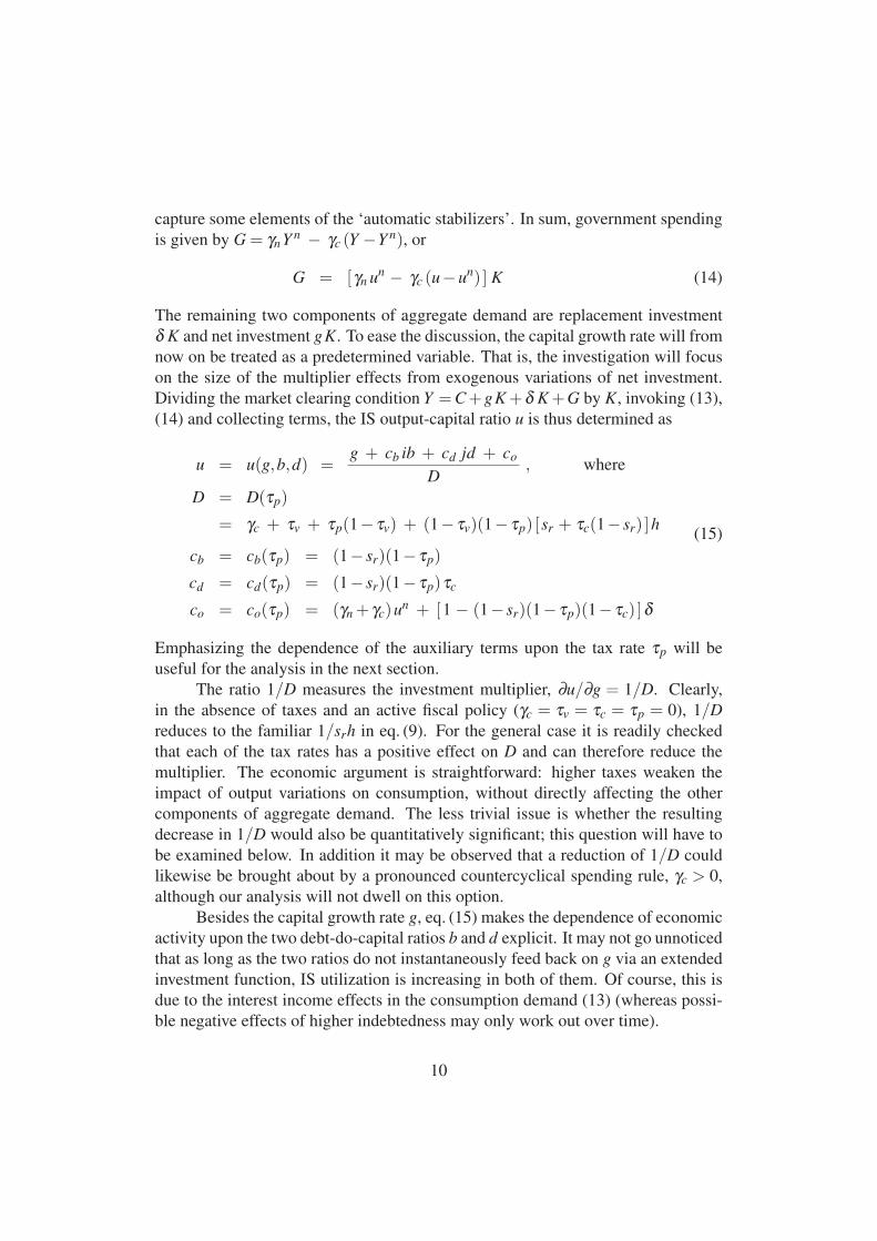
Dividing the market clearing condition Y = C +gK +δ K +G by K, invoking (13),

(14) and collecting terms, the IS output-capital ratio u is thus determined as

u = u(g,b,d) =g + cb ib + cd jd + co

D, where

D = D(τp)

= γc + τv + τp(1− τv) + (1− τv)(1− τp) [sr + τc(1− sr) ]h

cb = cb(τp) = (1− sr)(1− τp)

cd = cd(τp) = (1− sr)(1− τp)τc

co = co(τp) = (γn + γc)un + [1 − (1− sr)(1− τp)(1− τc) ]δ

(15)

Emphasizing the dependence of the auxiliary terms upon the tax rate τp will be

useful for the analysis in the next section.

The ratio 1/D measures the investment multiplier, ∂u/∂g = 1/D. Clearly,

in the absence of taxes and an active fiscal policy (γc = τv = τc = τp = 0), 1/D

reduces to the familiar 1/srh in eq. (9). For the general case it is readily checked

that each of the tax rates has a positive effect on D and can therefore reduce the

multiplier. The economic argument is straightforward: higher taxes weaken the

impact of output variations on consumption, without directly affecting the other

components of aggregate demand. The less trivial issue is whether the resulting

decrease in 1/D would also be quantitatively significant; this question will have to

be examined below. In addition it may be observed that a reduction of 1/D could

likewise be brought about by a pronounced countercyclical spending rule, γc > 0,

although our analysis will not dwell on this option.

Besides the capital growth rate g, eq. (15) makes the dependence of economic

activity upon the two debt-do-capital ratios b and d explicit. It may not go unnoticed

that as long as the two ratios do not instantaneously feed back on g via an extended

investment function, IS utilization is increasing in both of them. Of course, this is

due to the interest income effects in the consumption demand (13) (whereas possi-

ble negative effects of higher indebtedness may only work out over time).

10

4 The steady state position

The output-capital ratio in (15) cannot be readily interpreted as a long-run equilib-

rium solution. For that, it has to be taken into account that the two debt ratios b and

d follow an intrinsic dynamics, so that also u = u(g,b,d) will not remain constant.

The ratios are generally varying in the course of time because the firms have to

borrow D to finance investment, and the government has to issue new bonds B to

finance its deficit. This feature prompts us to identify the rest points of b and d, even

though as yet no complete full-fledged model has been set up. For the framework to

be meaningful, it should moreover be checked whether the conditional adjustment

processes are stable for each of the variables (i.e., conditional on the assumption

that the other variables stay put).

Let us begin with the debt dynamics of the business sector. In addition to the

assumption that the firms pay out all of their profits to the shareholders, we follow

much of the literature and (explicitly) assume a constant number of equities.10 Net

investment is thus exclusively financed by raising new credits, g pK = D. As d =d(D/pK)/dt = D/pK− (π +g)d (where π := p = p/p is the constant rate of price

inflation), we have

d = g − (g+π)d (16)

As long as the growth rate g+π of the nominal output is positive, these adjustments

are stable. Working with an exogenously given equilibrium level g = go of the

capital growth rate, process (16) is independent of the rest of the economy and the

debt-asset ratio converges to

do = go /(go +π) (17)

(Here and in the following, a superscript ‘o’ may indicate steady state values.)

Turning to the model’s implication for the government bonds, we first sum up the

10This assumption remains often implicit in the literature. It implies that stock prices must rise—

at least if in a steady state position the rentiers are required to allocate their wealth in fixed propor-

tions between equities, deposits and government bonds. For simplicity, the resulting capital gains

are not supposed to feed back on the real sector. Given that over most of the past three decades

US firms issued no new shares but rather bought them back from the market, a constant number of

equities appears an acceptable benchmark. For a more general framework it would have to be recog-

nized that the debt-to-capital ratio, the equity-to-capital ratio and Tobin’s q are not independent of

one another, so that further assumptions or specifications would have to be introduced; see Franke

and Yanovski (2015) for a more explicit treatment of these relationships in an otherwise elementary

framework.

11

(nominal) tax revenues T , normalized by the capital stock:

T/pK = τv u + τp(1− τv)(1−h)u + τp(1− τc)[(1− τv)hu−δ − jd] +

τp jd + τp ib + τc [(1− τv)hu−δ − jd]

= {τv + (1− τv)[τp + τc(1− τp)h]} u +

τp ib − τc(1− τp) jd − [τc + τp(1− τc)]δ

(18)

The first term after the first equals sign represents the taxes on the gross value

added, the second the taxes on wages, the third the taxes on the dividend payments,

the fourth and fifth the taxes on the rentiers’ interest income from their deposits

and government bonds, respectively, and the sixth term lastly captures the taxes on

corporate income.

The financing of the government deficit by new bonds gives rise to a second

dynamic equation, B = pG + iB−T . From b = d(B/pK)/dt = B/pK− (π + g)btogether with eqs (14) and (18), the following differential equation for the bond

ratio is obtained:

b = [(1−τp) i−g−π]b + τc(1− τp) jd + [τc + τp(1− τc)]δ +

(γn + γc)un − {γc + τv + (1− τv)[τp + τc(1− τp)h]} u(g,b,d)(19)

Because government bonds are relatively safe, the after-tax bond rate (1−τp)ishould not exceed the nominal growth rate g + π . Since furthermore utilization

u = u(g,b,d) is increasing in b, we can be rather sure of a negative derivative

∂b/∂b < 0. That is, the bond dynamics when taken on its own is a stable adjustment

process, too.

Going back to eq. (18) for the tax collections and neglecting a possible coun-

tercyclical fiscal policy (γc = 0), the ratio of the primary deficit to GDP in a state

where b = 0 is readily seen to be given by

pG

pY−

T

pY= γn

un

u−

T

pY= (go + π − i)b/u (20)

As the difference between go + π and the (pre-tax) bond rate will be rather small,

the (full) government deficit will essentially amount to the interest payments, that

is, we have deficit/pY = (pG + iB− T )/pY ≈ iB/pY . With familiar figures (in

former times) like i = 5% and B/pY = 60%, we also get a familiar deficit ratio of

3%.

The present set-up can already be used to analyze certain elementary issues of

a so-called ‘functional finance’, the theory of which goes back to Lerner (1943) and

still remains influential in the contemporary post-Keynesian work on fiscal policy

12

and public debt. Therefore, before turning to a numerical calibration of the model

components, we devote the rest of this section to a policy problem that was recently

addressed by Ryoo and Skott (2013, 2015) within a similar modelling framework,

when they were concerned with the necessary long-run requirements for a full-

employment growth path. In this context one asks for suitable combinations of the

government consumption coefficient γn, the tax rates τv, τc, τp, and the equilibrium

debt ratio bo that can bring about a given natural growth rate go and a given level

un of normal utilization.11 Ryoo and Skott (2013, pp. 518f; 2015, Section 2.3)

obtain two at first sight striking implications of their analysis. First, a reduction of

government consumption necessarily increases (rather than decreases) the long-run

debt ratio. Second, a higher natural growth rate lowers the required debt ratio.12

For a more detailed assessment of these statements it has, however, to be added

that these changes go along with adjustments in the tax rate on personal income. In

particular, the first result is less astonishing if it is realized that the lower spending

ratio γn allows the government to reduce taxes.

Treating their coefficient of government consumption as given, Ryoo and

Skott compute the steady state values of the debt ratio bo and their income tax

rate τ (which is their only tax rate) in a two-step procedure. First, they can solve

the model for bo, where interestingly this value turns out to be independent of τ .

The tax rate compatible with go and u = un is calculated subsequently and has bo

as one of its determinants. Things are not so straightforward in the present model.

If we fix the government spending ratio γn and the two tax rates τv and τc, the equi-

librium values of the debt ratio b and the remaining tax rate τp on personal income

are mutually dependent.

We tackle this problem by devising two steady state relationships where b

can be formally written as a function of τp. One of them is increasing, the other

decreasing, and their point of intersection yields the unique long-run equilibrium

pair (bo,τp). The first function is obtained by reversing the causality in the IS

equation. We thus focus on the values of b that support normal utilization under

variations of τp. Accordingly, we fix u = un on the left-hand side of (15) together

with d = do on the right-hand side and, making use of the terms D = D(τp), etc.,

solve this equation for b. Referring to these values as b = boIS(τp), our first function

11The natural growth rate is then, of course, determined by the growth of productivity and the

labour force. In addition to b = 0 and uo = un, full employment in a steady state will prevail if

another condition on the ratio of the capital stock to the labour force is fulfilled (Ryoo and Skott,

2015, p. 11).12As noted by Ryoo and Skott (2015, fn 11 on p. 11), similar results have also previously been

obtained in other settings.

13

reads,

boIS(τp) =

D(τp)un − go − cd(τp) jdo − co(τp)

cb(τp) i(21)

The second relationship derives from the government debt dynamics. It is con-

cerned with the values of b and τp that bring about b = 0 in (19), where u = u(go,bo,do) = un is already presupposed to prevail, besides d = do. The solution of this

equation for the debt ratio provides us with a second function b = boGD(τp) (the

index ‘GD’ may stand for government debt),

boGD(τp) =

a1(τp) − a2(τp)un + γn un

a3(τp)

a1 = a1(τp) = τc(1− τp) jdo + [τc + τp(1− τc)]δ

a2 = a2(τp) = τv + (1− τv) [τp + τc(1− τp)h]

a3 = a3(τp) = go + π − (1− τp) i

(22)

It is spelled out in the appendix that the numerator of (21) is increasing in τp, while

the denominator is obviously decreasing. Hence boIS is an increasing function of

the tax rate τp. For boGD the opposite applies: its numerator is decreasing and its

denominator increasing in τp, so that boGD decreases with rising values of τp.

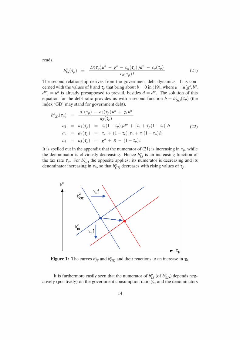
Figure 1: The curves boIS and bo

GD and their reactions to an increase in γn.

It is furthermore easily seen that the numerator of boIS (of bo

GD) depends neg-

atively (positively) on the government consumption ratio γn, and the denominators

14

of (21) and (22) are both independent of it. Referring to the (τp,b) plane with the

tax rate on the horizontal axis, we can thus say that an increase in γn shifts the curve

boIS downward and the curve bo

GD upward (or to the right). As illustrated in Figure

1, the new point of intersection of the two curves will therefore lead to a higher

tax rate τp, whereas we get no unambiguous conclusion for the equilibrium debt

ratio bo: whether it increases or decreases depends on how far the curves will shift

relatively to one another. Figure 1 depicts a situation with a moderately lower debt

ratio. This is in fact the outcome that we obtain from the numerical values that will

be introduced in the next section. Note that this reaction corresponds to the result

by Ryoo and Skott (2013, 2015) mentioned above.13

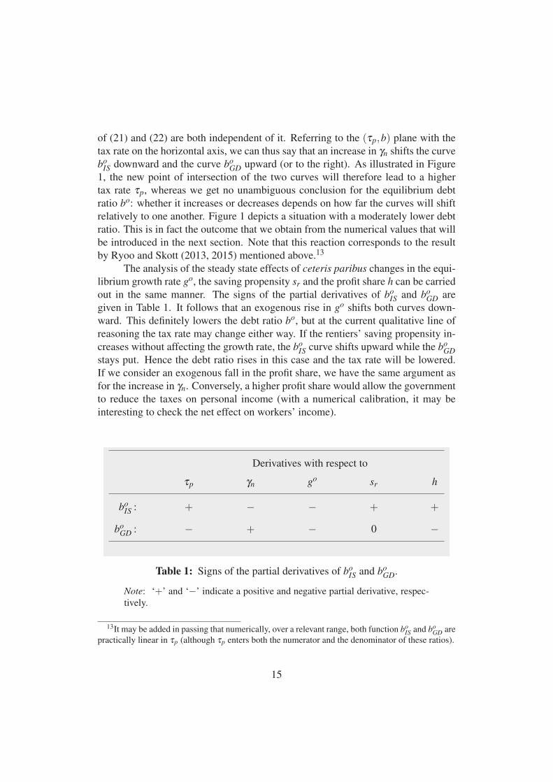
The analysis of the steady state effects of ceteris paribus changes in the equi-

librium growth rate go, the saving propensity sr and the profit share h can be carried

out in the same manner. The signs of the partial derivatives of boIS and bo

GD are

given in Table 1. It follows that an exogenous rise in go shifts both curves down-

ward. This definitely lowers the debt ratio bo, but at the current qualitative line of

reasoning the tax rate may change either way. If the rentiers’ saving propensity in-

creases without affecting the growth rate, the boIS curve shifts upward while the bo

GD

stays put. Hence the debt ratio rises in this case and the tax rate will be lowered.

If we consider an exogenous fall in the profit share, we have the same argument as

for the increase in γn. Conversely, a higher profit share would allow the government

to reduce the taxes on personal income (with a numerical calibration, it may be

interesting to check the net effect on workers’ income).

Derivatives with respect to

τp γn go sr h

boIS : + − − + +

boGD : − + − 0 −

Table 1: Signs of the partial derivatives of boIS and bo

GD.

Note: ‘+’ and ‘−’ indicate a positive and negative partial derivative, respec-

tively.

13It may be added in passing that numerically, over a relevant range, both function boIS and bo

GD are

practically linear in τp (although τp enters both the numerator and the denominator of these ratios).

15

These steady state comparisons should nevertheless be taken with care. Given

that realistically tax rates are not easily adjusted, the discussion may rather suggest

that at least for a longer period of time the economy will not be able to reach such a

state of long-run consistency. A more careful investigation of this problem is, how-

ever, beyond the present limited framework and would require a more elaborated

dynamic model, which is a challenge for future research.

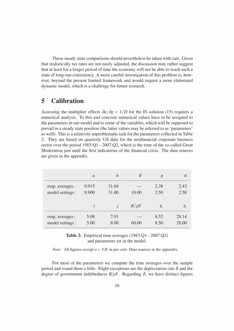
5 Calibration

Assessing the multiplier effects ∂u/∂g = 1/D for the IS solution (15) requires a

numerical analysis. To this end concrete numerical values have to be assigned to

the parameters in our model and to some of the variables, which will be supposed to

prevail in a steady state position (the latter values may be referred to as ‘parameters’

as well). This is a relatively unproblematic task for the parameters collected in Table

2. They are based on quarterly US data for the nonfinancial corporate business

sector over the period 1983:Q1 – 2007:Q2, which is the time of the so-called Great

Moderation just until the first indications of the financial crisis. The data sources

are given in the appendix.

u h δ g π

emp. averages : 0.915 31.04 — 2.38 2.43

model settings : 0.900 31.00 10.00 2.50 2.50

i j B/pY τv τc

emp. averages : 5.08 7.91 — 8.52 28.14

model settings : 5.00 8.00 60.00 8.50 28.00

Table 2: Empirical time averages (1983:Q1 – 2007:Q2)

and parameters set in the model.

Note: All figures except u = Y/K in per cent. Data sources in the appendix.

For most of the parameters we compute the time averages over the sample

period and round them a little. Slight exceptions are the depreciation rate δ and the

degree of government indebtedness B/pY . Regarding δ , we have distinct figures

16

from two data sets and choose a value somewhere in the middle. Regarding B/pY ,

figures differ according to the underlying statistical concepts. Here we just choose

a familiar order of magnitude for the time before the crisis.14 In addition, we set

γc = 0 since our multiplier effects should not depend on special assumptions on a

countercyclical fiscal policy (for higher aspirations, the appendix sketches a way to

obtain reasonable (positive) values for γc).

It may be mentioned as an aside that according to its definition in (11), the

values for u, h, δ imply a profit rate of r = 15.53%. The interest burden of the

government amounts to iB/pY = 0.05 · 0.60 = 3% of the economy’s total income.

Since the nominal growth rate go +π happens to equal the bond rate i, eq. (20) tells

us that the government has a balanced primary budget, pG = T . In other words, its

deficit is just made up of its interest payments. A deficit of 3% is also quite close to

the empirical time average.

The government’s debt-to-capital ratio in the equilibrium is b = bo = B/pK =(B/pY )(pY/pK) = 0.60 ·0.90 = 0.54. Regarding the private sector, the debt-asset

ratio of the firms in a steady state is d = do = go/(go +π) = 0.50; see eq. (17).15

Three parameters are thus remaining: the rentiers’ saving propensity sr, the

government’s normal spending ratio γn = Gn/Y n, and the tax rate τp on personal

income. The latter two parameters are interrelated if the government is to keep

its deficit within bounds. Supposing that normal utilization u = un prevails in a

long-run equilibrium, γn is obtained as a linear function of τp by setting b = 0 and

u(g,b,d) = un in eq. (19). Subsequently the saving propensity sr, which does not

show up in (19), can be determined from the goods market equilibrium. That is, the

expression u(go,bo,do) in (15) is set equal to un = 0.90 and, with τp and γn given,

the equation is solved for sr. Schematically,

γn(19)= γn(τp) and sr

(15)= sr(τp,γn) (23)

On this basis, we vary the tax rate τp, compute the corresponding values of γn and

sr, and check the implications of these numerical scenarios. In the first instance

we are, of course, interested in the resulting investment multiplier ∂u/∂g = 1/D;

D as determined in (15). A numerical target value that we would like the model

to achieve is readily derived as follows. From the data described in the appendix

we take the quarterly time series of the (annualized) capital growth rate gt and the

output-capital ratio ut and detrend them by the Hodrick-Prescott filter.16 Comput-

ing for these trend deviations gt , ut the standard deviations σ(gt) and σ(ut) over

14See, e.g., http://en.wikipedia.org/wiki/National debt of the United States

(July 2015).15Obviously, the ratio would be lower if the firms retain some of their earnings.16The conventional smoothing parameter is λ = 1600 for quarterly data. This is actually not fully

appropriate in the present case because the HP-trend of ut still exhibits some variability at a business

17

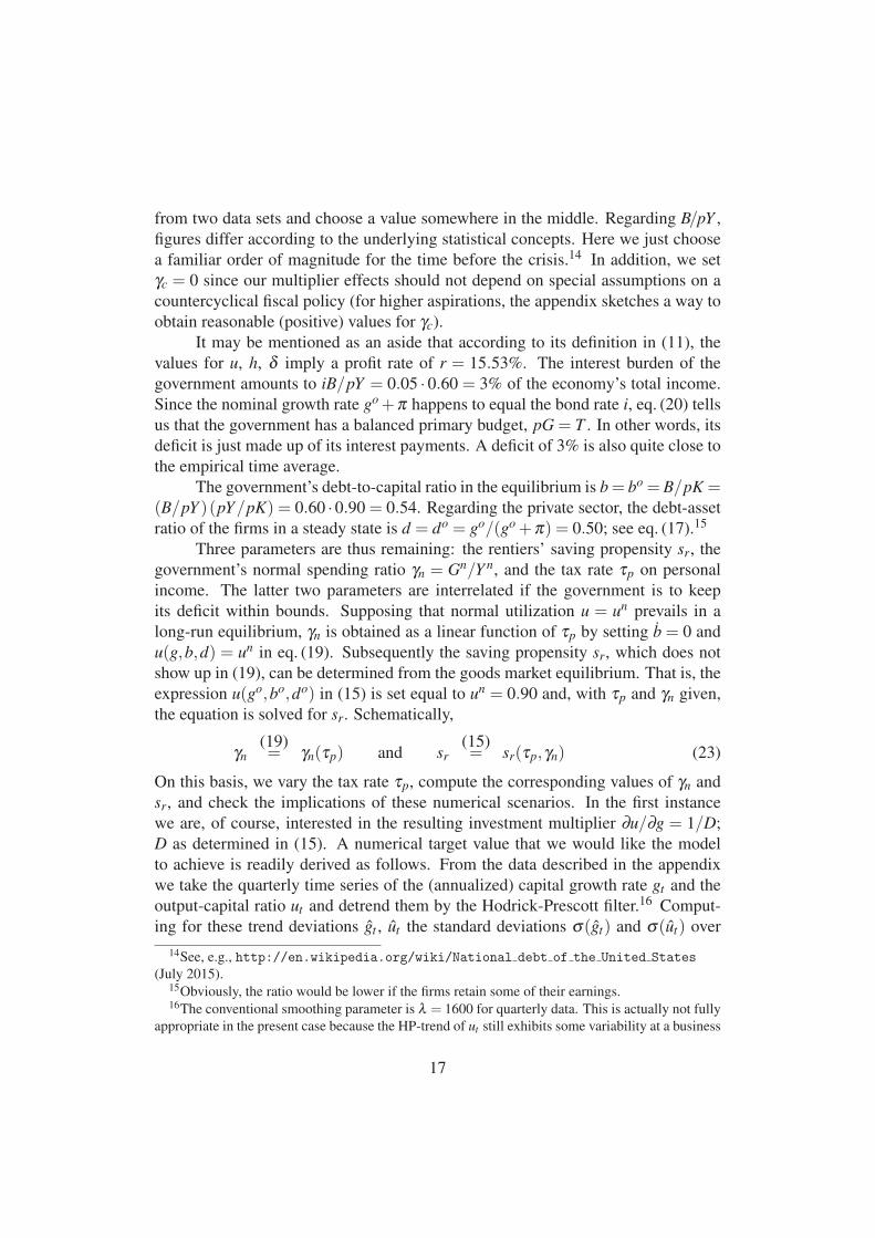
the abovementioned sample period, we employ the ratio σ(ut)/σ(gt) as our bench-

mark for the multiplier ∂u/∂g. This is the value given in the right column of Table

3. The fact that this statistic turns out to be more than ten times lower than the

value in (9) for the tax-less economy is already sufficient evidence that the simple

modelling framework does have a problem when it comes to elementary numerical

inspections.

T/pY ∂u/∂g

emp. averages : 28.60 2.20

benchmark values : 28.50 2.20

Table 3: Empirical time averages (1983:Q1 – 2007:Q2)

and model benchmark values.

Reasonable multiplier effects should not be the only concern in our effort to

calibrate the model. At the same time the tax payments, or what amounts to the

same: the government spending, should not get out of range. We thus take the

tax-to-income ratio T/pY in Table 3 as a second benchmark. For the model we can

invoke eq. (18) and compute it as T/pY = (T/pK) ·un.

Because of its analogy to the estimation approach known as the method of

simulated moments (Lee and Ingram, 1991; Franke, 2009), which will immedi-

ately become apparent, the two statistics ∂u/∂g and T/pY may also be referred to

as ‘moments’. The first, for short, is our multiplier moment and the second our

tax moment, and their desired values may be denoted as (∂u/∂g)d and (T/pY )d ,

respectively. If at all, we cannot expect that variations of a single parameter like

τp will be able to match both of them. Generally, we are in search of a value of τp

such that the thus generated moments come as close as possible to the desired mo-

ments. To quantify this “as close as possible”, we introduce a weighting coefficient

ω (0≤ ω ≤ 1) and set up a first objective function, or loss function, that expresses

the quality of the match in percentage terms:

L1,ω = ω |DevM| + (1−ω) |DevT | (24)

cycle frequency. A stronger smoothing is necessary to let it disappear. We actually decided on

λ = 51,200, which is 25 times higher than the standard value.

18

:= ω∣

∣

∣

100 · [∂u/∂g − (∂u/∂g)d]

(∂u/∂g)d

∣

∣

∣+ (1−ω)

∣

∣

∣

100 · [T/pY − (T/pY )d]

(T/pY )d

∣

∣

∣

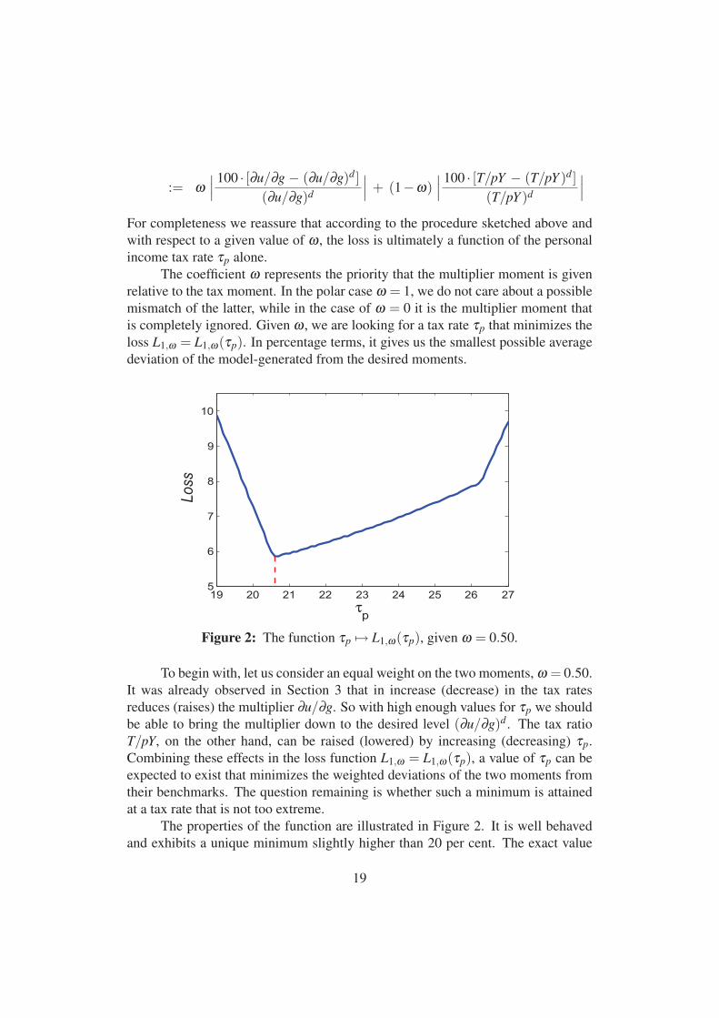
For completeness we reassure that according to the procedure sketched above and

with respect to a given value of ω , the loss is ultimately a function of the personal

income tax rate τp alone.

The coefficient ω represents the priority that the multiplier moment is given

relative to the tax moment. In the polar case ω = 1, we do not care about a possible

mismatch of the latter, while in the case of ω = 0 it is the multiplier moment that

is completely ignored. Given ω , we are looking for a tax rate τp that minimizes the

loss L1,ω = L1,ω(τp). In percentage terms, it gives us the smallest possible average

deviation of the model-generated from the desired moments.

19 20 21 22 23 24 25 26 275

6

7

8

9

10

τp

Loss

Figure 2: The function τp 7→ L1,ω(τp), given ω = 0.50.

To begin with, let us consider an equal weight on the two moments, ω = 0.50.

It was already observed in Section 3 that in increase (decrease) in the tax rates

reduces (raises) the multiplier ∂u/∂g. So with high enough values for τp we should

be able to bring the multiplier down to the desired level (∂u/∂g)d . The tax ratio

T/pY, on the other hand, can be raised (lowered) by increasing (decreasing) τp.

Combining these effects in the loss function L1,ω = L1,ω(τp), a value of τp can be

expected to exist that minimizes the weighted deviations of the two moments from

their benchmarks. The question remaining is whether such a minimum is attained

at a tax rate that is not too extreme.

The properties of the function are illustrated in Figure 2. It is well behaved

and exhibits a unique minimum slightly higher than 20 per cent. The exact value

19

is τp = 20.57% (rounded). This rate brings about an average moment deviation

of L1,ω = 5.83%, but the single matches are rather distinct. The tax moment is

actually perfectly matched, DevT = 0, whereas the multiplier moment deviates by

L1,ω/ω = 5.83/ω = 11.66% from the desired multiplier, that is, ∂u/∂g = 2.46

versus the desired value of 2.20. Given the order of magnitude for the investment

multiplier in the taxless economy, this is certainly a remarkable progress.

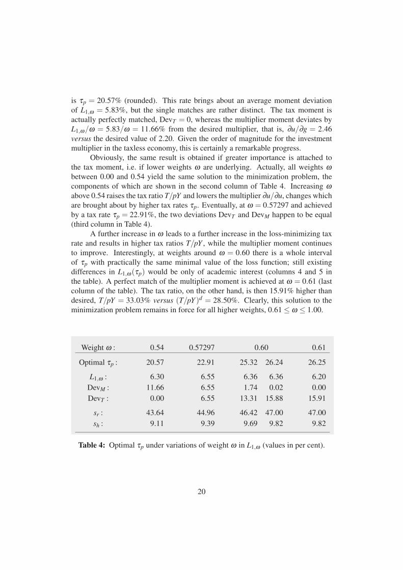
Obviously, the same result is obtained if greater importance is attached to

the tax moment, i.e. if lower weights ω are underlying. Actually, all weights ωbetween 0.00 and 0.54 yield the same solution to the minimization problem, the

components of which are shown in the second column of Table 4. Increasing ωabove 0.54 raises the tax ratio T/pY and lowers the multiplier ∂u/∂u, changes which

are brought about by higher tax rates τp. Eventually, at ω = 0.57297 and achieved

by a tax rate τp = 22.91%, the two deviations DevT and DevM happen to be equal

(third column in Table 4).

A further increase in ω leads to a further increase in the loss-minimizing tax

rate and results in higher tax ratios T/pY , while the multiplier moment continues

to improve. Interestingly, at weights around ω = 0.60 there is a whole interval

of τp with practically the same minimal value of the loss function; still existing

differences in L1,ω(τp) would be only of academic interest (columns 4 and 5 in

the table). A perfect match of the multiplier moment is achieved at ω = 0.61 (last

column of the table). The tax ratio, on the other hand, is then 15.91% higher than

desired, T/pY = 33.03% versus (T/pY )d = 28.50%. Clearly, this solution to the

minimization problem remains in force for all higher weights, 0.61≤ ω ≤ 1.00.

Weight ω : 0.54 0.57297 0.60 0.61

Optimal τp : 20.57 22.91 25.32 26.24 26.25

L1,ω : 6.30 6.55 6.36 6.36 6.20

DevM : 11.66 6.55 1.74 0.02 0.00

DevT : 0.00 6.55 13.31 15.88 15.91

sr : 43.64 44.96 46.42 47.00 47.00

sh : 9.11 9.39 9.69 9.82 9.82

Table 4: Optimal τp under variations of weight ω in L1,ω (values in per cent).

20

The next-to-last row in Table 4 reports the rentiers’ saving propensity sr as-

sociated with the optimal solutions. It is consistently more than three times higher

than the value of 14% in the taxless scenario underlying the multiplier in eq. (9).

The higher propensity will also seem sociologically more plausible. We can never-

theless have an another check by referring to the aggregate saving propensity sh for

all private households, rentiers and the non-saving workers together. With dispos-

able income Y d and obvious indices r and w for the two groups,

Y dr = (1− τp){(1− τc) [(1− τv)hun−δ − jdo]+ jdo + ibo } pK

Y dw = (1− τp)(1− τv)(1−h)un pK

sh is given by

sh = sr Y dr /(Y d

r + Y dw ) (25)

The last row in Table 4 demonstrates that this propensity is between nine and ten

per cent. While historically in the US the personal saving rate was lower than that

over the last few decades, it may be brought into consideration that these times were

not very close to a balanced growth path and there was often quite some concern

about insufficient savings of the households. It is remarkable in this respect that the

rate showed a declining trend from 12.5% in the early 1980s down to 2.5% around

2005, and that between 1960 and 1980 it fell below the 10% mark for only short

intermediate periods.17 The nine to ten per cent range for our sh should therefore

be well acceptable.

Back to the taxes, another feature of the plausibility of the model and its

results are the shares of the single tax categories in the total tax revenues. For a

rough-and-ready check let us consider the taxes on corporate income, Tc, versus

the sum of payroll and individual income taxes, designated Tp. The latter are, of

course, the dominating category. In number, regarding the federal tax receipts, Tp

comprised 88% of (Tp + Tc) in the year 2014.18 In the model, we obtain Tp/(Tp +Tc) = 82.1% for the first tax rate τp = 20.57% in Table 4. Clearly, the proportion

will rise if the optimal τp rises with the weight in the loss function. For τp = 26.25%

in the last column of the table, the proportion reaches Tp/(Tp + Tc) = 85.4%. We

can thus say that also in the composition of the main taxes, the model exhibits no

dramatic deviations from the empirical data.19

17See the website of the Federal Reserve Bank of St. Louis (Economic Research) about the per-

sonal saving rate, https://research.stlouisfed.org/fred2/series/PSAVERT (July 2015).18See http:/en.wikipedia.org/wiki/Taxation in the United States (Levels and

types of taxation; July 2015). For our model, Tc is captured by the last term in the first part of

eq. (18), and Tp by the terms 2 – 5.19If one attaches greater importance to this criterion, one could introduce Tp/(Tp + Tc) and a

desired value of it as a third moment in the loss function, furnished with a weight reflecting the

researcher’s priority.

21

6 Moderate improvements in the moment matching

Although the results make good economic sense so far, there is always the question

for something better. While one cannot expect that the variations of one parameter,

the personal income tax rate τp in the previous section, would be able to bring about

a perfect match of two moments, what about treating another coefficient as a free

parameter? Let us therefore examine the effects of the corporate tax rate τc in this

respect.

Underlying the quantitative evaluation of the moment matching is the weight

ω in the loss function (24). To organize the discussion we consider three benchmark

cases: first ω = 0, which under suitable variations of at least one of the parameters

will ensure us a perfect match of the tax moment, and we now want to study possible

improvements in the multiplier moment; second ω = 1, where the roles of the two

moments are interchanged. In a third case we are interested in situations with a

symmetric mismatch of the two moments. In all three cases we let τc exogenously

vary over a range between 20 and 32 per cent, and for each such τc compute the

value of τp that minimizes the corresponding loss function. The question that we

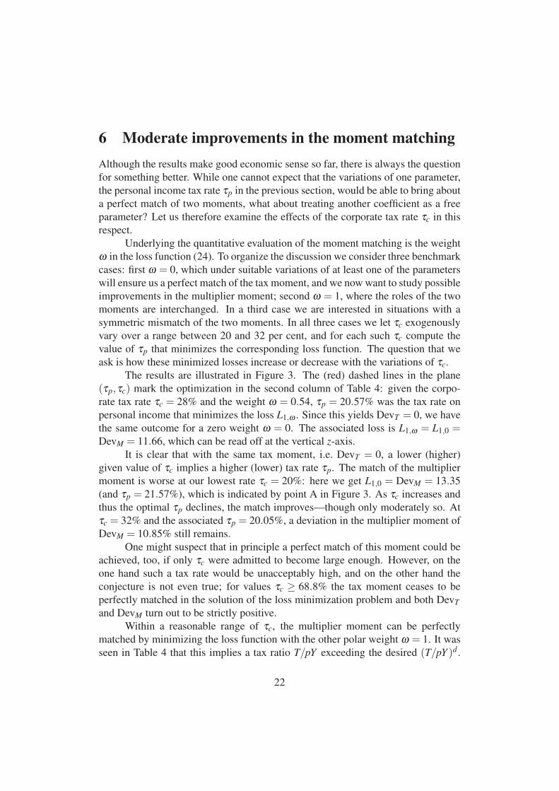
ask is how these minimized losses increase or decrease with the variations of τc.

The results are illustrated in Figure 3. The (red) dashed lines in the plane

(τp,τc) mark the optimization in the second column of Table 4: given the corpo-

rate tax rate τc = 28% and the weight ω = 0.54, τp = 20.57% was the tax rate on

personal income that minimizes the loss L1,ω . Since this yields DevT = 0, we have

the same outcome for a zero weight ω = 0. The associated loss is L1,ω = L1,0 =DevM = 11.66, which can be read off at the vertical z-axis.

It is clear that with the same tax moment, i.e. DevT = 0, a lower (higher)

given value of τc implies a higher (lower) tax rate τp. The match of the multiplier

moment is worse at our lowest rate τc = 20%: here we get L1,0 = DevM = 13.35

(and τp = 21.57%), which is indicated by point A in Figure 3. As τc increases and

thus the optimal τp declines, the match improves—though only moderately so. At

τc = 32% and the associated τp = 20.05%, a deviation in the multiplier moment of

DevM = 10.85% still remains.

One might suspect that in principle a perfect match of this moment could be

achieved, too, if only τc were admitted to become large enough. However, on the

one hand such a tax rate would be unacceptably high, and on the other hand the

conjecture is not even true; for values τc ≥ 68.8% the tax moment ceases to be

perfectly matched in the solution of the loss minimization problem and both DevT

and DevM turn out to be strictly positive.

Within a reasonable range of τc, the multiplier moment can be perfectly

matched by minimizing the loss function with the other polar weight ω = 1. It was

seen in Table 4 that this implies a tax ratio T/pY exceeding the desired (T/pY )d .

22

20

25

3020

2224

2628

5

10

15

20

τc

B

C

L11

A

L2

τp

L10

Loss

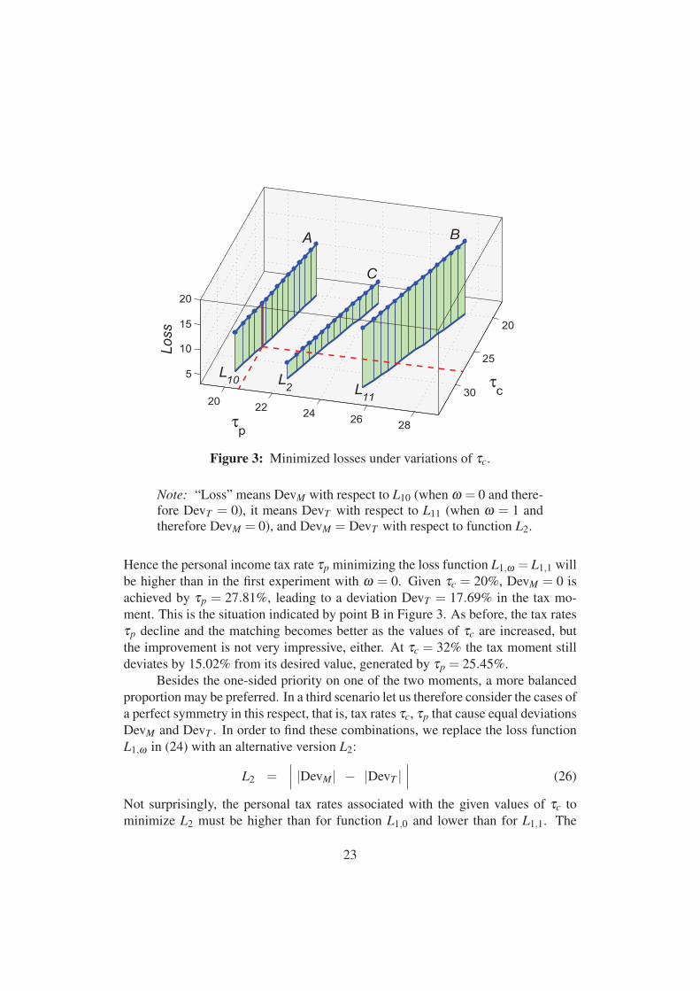
Figure 3: Minimized losses under variations of τc.

Note: “Loss” means DevM with respect to L10 (when ω = 0 and there-

fore DevT = 0), it means DevT with respect to L11 (when ω = 1 and

therefore DevM = 0), and DevM = DevT with respect to function L2.

Hence the personal income tax rate τp minimizing the loss function L1,ω = L1,1 will

be higher than in the first experiment with ω = 0. Given τc = 20%, DevM = 0 is

achieved by τp = 27.81%, leading to a deviation DevT = 17.69% in the tax mo-

ment. This is the situation indicated by point B in Figure 3. As before, the tax rates

τp decline and the matching becomes better as the values of τc are increased, but

the improvement is not very impressive, either. At τc = 32% the tax moment still

deviates by 15.02% from its desired value, generated by τp = 25.45%.

Besides the one-sided priority on one of the two moments, a more balanced

proportion may be preferred. In a third scenario let us therefore consider the cases of

a perfect symmetry in this respect, that is, tax rates τc, τp that cause equal deviations

DevM and DevT . In order to find these combinations, we replace the loss function

L1,ω in (24) with an alternative version L2:

L2 =∣

∣

∣|DevM| − |DevT |

∣

∣

∣(26)

Not surprisingly, the personal tax rates associated with the given values of τc to

minimize L2 must be higher than for function L1,0 and lower than for L1,1. The

23

precise outcome is shown in the middle of Figure 3. Beginning at point C, where

τc = 20% is given, the tax rate τp = 24.17% brings about equal deviations DevM =DevT = +7.37%. Again, they can be made smaller by increasing τc. At τc = 32%,

then, τp = 22.26% can reduce the joint mismatch to DevM = DevT = +6.14%.

The following four points may briefly summarize what we learn from the

three experiments underlying Figure 3.

• A perfect match of both the tax and the multiplier moment is not possible.

• While better matches are possible by increasing the corporate tax rate τc, the

improvement is rather limited.

• Which pair (τc,τp) a researcher may choose in his or her practical work can

therefore mainly depend on his/her personal preferences regarding the two

moments or the values of the tax rates τc and τp directly.

• In all cases within the range of the tax rates discussed here, the quality of the

moment matching can be considered fairly satisfactory, except perhaps for

the deviations between 15% and 17.7% in the tax moment (in the right part

of Figure 3).

While with respect to our two moments the parameter combinations discussed

here may appear entirely satisfactory, they may turn out to be less suitable when

the present model components are integrated into a wider framework and one is

interested in additional dynamic properties. The idea of moment matching can,

however, be readily extended to such more ambitious models; simply include the

relevant summary statistics as additional moments in the loss function, specify a

number of free parameters, and solve the corresponding loss minimization problem.

Franke et al. (2015) and Jang and Sacht (2015) are two examples that show that this

approach can be successfully used to estimate (not only asset pricing models but

also) fully-fledged dynamic macro models in general.

7 A cyclical scenario

When discussing the strong multiplier effects arising in equations (5) or (9) for the

taxless economy in Section 2, reference was also made to possible difficulties in

cyclical economies. In particular, it was mentioned that the amplitudes of the debt-

to-capital ratios in models of this type may be unrealistically low in relation to the

oscillations in utilization. In order to indicate the relevance of this problem, we

give a couple of examples from elaborated, mostly recent contributions that are so

ambitious as to include a detailed numerical analysis.

24

(i) While the motions of utilization are acceptable in Flaschel et al. (1997, p. 368;

FFS in the following), their capital growth rate oscillates with an amplitude of

just±0.26% around its long-run equilibrium value of 3.50%, and the business

debt-to-capital ratio with ±0.10% around 30.00% (see also p. 365).

(ii) In Lojak (2014, p. 35) the amplitude of the firms’ debt-asset ratio is ±0.24%

around the same 30.00% and the capital growth rate oscillates with g =3.000%± 0.085% (utilization is again acceptable). Although the model has

a similar financial sector to the former reference, the debt-asset ratio behaves

qualitatively differently: in FFS it lags behind utilization whereas in Lojak

(2014) it turns out to be a leading variable.20

(iii) From the diagrams in Nikolaidi (2014, p. 10) one can infer regular oscillations

of 0.70±0.10 for her rate of capacity utilization, 4%±1.30% for the capital

growth rate, and 18.85%±0.25% for the firms’ debt-asset ratio. For a better

comparison with the previous results we do a rough calculation and scale

utilization down to 0.700± (3 per cent of 0.700) = 0.700±0.021. Adjusting

the other two variables proportionately, the capital growth rate would move

like 4%± (0.021/0.10) ·1.30% = 4.000%±0.273% and the debt-asset ratio

like 18.8500%±0.0525%.

(iv) From Schoder (2014, p. 19), an amplitude of approximately 0.70± 0.15 for

the output-capital ratio and of 45%± 8% for the debt-asset ratio can be in-

ferred. Scaling these motions down as before, we have 0.700±0.021 for the

former and 45%± (0.021/0.15) ·8% = 45.00%±1.13%. This order of mag-

nitude is much better than in the other examples but not fully trustworthy,

either, because the equilibrium value of his capital growth rate is as high as

g = 21.42%.21

(v) A similar problem arises in the estimations by Hein and Schoder (2011), as

a result of which they obtain reasonable IS multiplier effects. However, if

one plugs the empirical long-term averages of several key variables for the

20One reason responsible for this outcome are different assumptions about inflation. Further

insights can be gained from the stylized experiments in FFS, Chapter 13.3, and the discussion in

Lojak (2014, pp. 27f).21In detail and using Schoder’s notation one has g = gs = ζ uσ in his saving function (2), where

the parameters given in his Appendix B are ζ = 0.51, u = 0.70, σ = 0.60 and ζ is a composite

term involving a saving parameter s. If Schoder’s treatment is compared with what we did for our

back-of-the-envelope calculation for the multiplier equation (9) in Section 2, he assumes an a priori

plausible value for s and obtains the growth rate g in the saving function as a residual, whereas

we started out from a reasonable value for the steady state growth rate and determined our saving

propensity residually. We believe the latter procedure is preferable since the order of magnitude of

g is more reliable than that of a saving parameter.

25

US (Table 1, p. 702) and the estimated parameters (Table 8, p. 712) back into

the saving function of the theoretical model, one obtains a capital growth rate

higher than 20.9%.22

Against this background, we now want to get an impression of the cyclical features

that the present model with its moderate multiplier effects gives rise to. To this end

it suffices to treat the capital growth rate as an exogenous variable and to postulate a

deterministic stylized sine wave for it. Let its period be 8.50 years and its amplitude

g = 2.50%±1.17%. This specification results in a standard deviation of 0.83% over

one cycle, which equals the empirical standard deviation of this variable over the

period of the Great Moderation mentioned in Section 5.

Given the parameters of the model, this is all what is needed to set it in mo-

tion. The changes in the output-capital ratio u = u(g,b,d) are determined from the

IS solution (15) and the changes in the two debt ratios, which in turn are described

by the differential equations (16) and (19). Adopting the numerical parameters from

the calibration in Table 2 above, it remains to decide on the personal income tax rate

τp. Here we choose the rate that leads to identical deviations of the two moments

from the desired values. Under the exogenous variations of the corporate tax rate

τc, these situations are represented by L2 in Figure 3. With respect to τc = 28%

from Table 2, we can refer to the third column in Table 4:

τp = 22.91%, implying

{

∂u/∂g = 2.34, (T/pY )o = 30.37%

DevM = 6.55%, DevT = 6.55%(27)

Starting from the equilibrium values of d and b, and from g on the sine wave at

some arbitrary point in time, the economy after a while develops into a regular and

strictly periodic motion of all its variables. Figure 4 illustrates the amplitudes and

the comovements of utilization u and the capital growth rate g in the first panel

(the bold and thin line, respectively), and of the two ratios d and b in the other two

panels. The growth rate g is shifted upward here, so that it oscillates around the

same value as u and can directly be seen to move almost synchronously with that

measure of a business cycle. Clearly, u also has a larger amplitude than g. The

debt-asset ratio of the firm sector lags utilization by approximately one quarter of

22Because data on the dividend payments to the rentiers (which show up in their framework) are

not reported in the paper, we helped ourselves by conservatively assuming that they are three times

higher than the interest receipts; realistically lower dividends would only increase the growth rate

still further. While the implied high growth rate goes unnoticed by the authors, they do mention that

the empirical output-capital ratio differs from the model’s IS solution (though without specifying the

numerical order of magnitude; see p. 712). However, they attribute the discrepancy to the effects of

cumulative stochastic noise in the estimations (see fn 37), which, as a short claim, does not appear a

very convincing excuse.

26

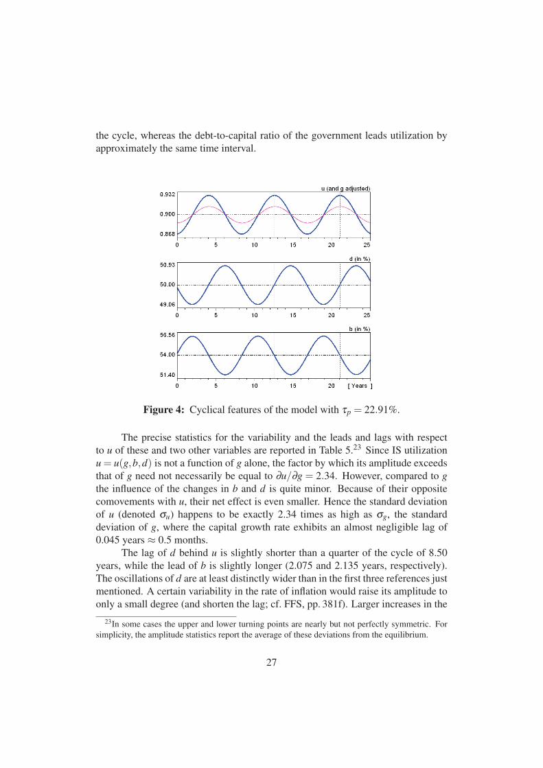
the cycle, whereas the debt-to-capital ratio of the government leads utilization by

approximately the same time interval.

Figure 4: Cyclical features of the model with τp = 22.91%.

The precise statistics for the variability and the leads and lags with respect

to u of these and two other variables are reported in Table 5.23 Since IS utilization

u = u(g,b,d) is not a function of g alone, the factor by which its amplitude exceeds

that of g need not necessarily be equal to ∂u/∂g = 2.34. However, compared to g

the influence of the changes in b and d is quite minor. Because of their opposite

comovements with u, their net effect is even smaller. Hence the standard deviation

of u (denoted σu) happens to be exactly 2.34 times as high as σg, the standard

deviation of g, where the capital growth rate exhibits an almost negligible lag of

0.045 years ≈ 0.5 months.

The lag of d behind u is slightly shorter than a quarter of the cycle of 8.50

years, while the lead of b is slightly longer (2.075 and 2.135 years, respectively).

The oscillations of d are at least distinctly wider than in the first three references just

mentioned. A certain variability in the rate of inflation would raise its amplitude to

only a small degree (and shorten the lag; cf. FFS, pp. 381f). Larger increases in the

23In some cases the upper and lower turning points are nearly but not perfectly symmetric. For

simplicity, the amplitude statistics report the average of these deviations from the equilibrium.

27

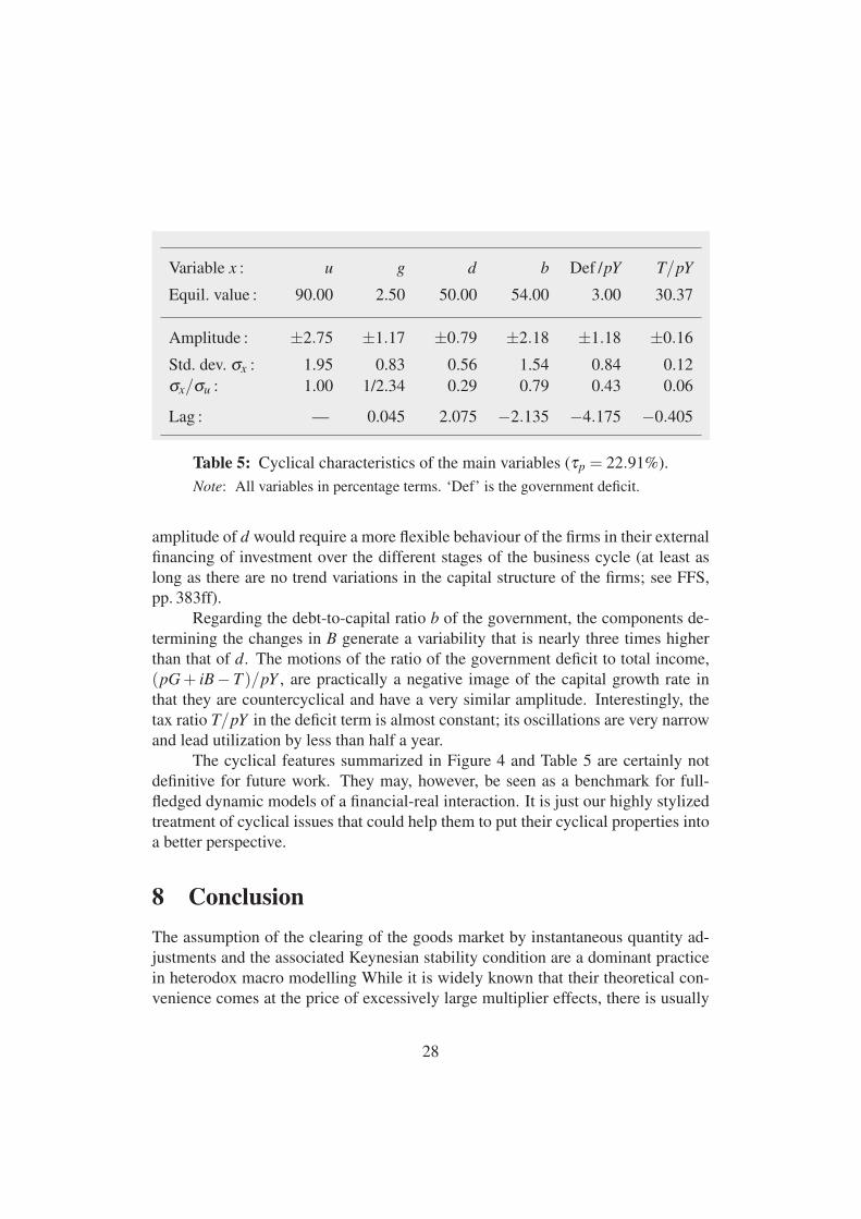
Variable x : u g d b Def /pY T/pY

Equil. value : 90.00 2.50 50.00 54.00 3.00 30.37

Amplitude : ±2.75 ±1.17 ±0.79 ±2.18 ±1.18 ±0.16

Std. dev. σx : 1.95 0.83 0.56 1.54 0.84 0.12

σx/σu : 1.00 1/2.34 0.29 0.79 0.43 0.06

Lag : — 0.045 2.075 −2.135 −4.175 −0.405

Table 5: Cyclical characteristics of the main variables (τp = 22.91%).

Note: All variables in percentage terms. ‘Def’ is the government deficit.

amplitude of d would require a more flexible behaviour of the firms in their external

financing of investment over the different stages of the business cycle (at least as

long as there are no trend variations in the capital structure of the firms; see FFS,

pp. 383ff).

Regarding the debt-to-capital ratio b of the government, the components de-

termining the changes in B generate a variability that is nearly three times higher

than that of d. The motions of the ratio of the government deficit to total income,

(pG + iB− T )/pY , are practically a negative image of the capital growth rate in

that they are countercyclical and have a very similar amplitude. Interestingly, the

tax ratio T/pY in the deficit term is almost constant; its oscillations are very narrow

and lead utilization by less than half a year.

The cyclical features summarized in Figure 4 and Table 5 are certainly not

definitive for future work. They may, however, be seen as a benchmark for full-

fledged dynamic models of a financial-real interaction. It is just our highly stylized

treatment of cyclical issues that could help them to put their cyclical properties into

a better perspective.

8 Conclusion

The assumption of the clearing of the goods market by instantaneous quantity ad-

justments and the associated Keynesian stability condition are a dominant practice

in heterodox macro modelling While it is widely known that their theoretical con-

venience comes at the price of excessively large multiplier effects, there is usually

28

little sincere concern about this problem. It may in fact be neglected as long as one

is only interested in the sign of the multipliers, but severe distortions with possibly

misleading implications will arise in quantitative work. Although more complex

models with, in particular, more detailed dynamic feedbacks might be able to avoid

the problem, they are no longer easily related to the results from the ordinary mod-

els, so to speak; quite apart from the fact that here no canonical framework has been

developed so far.

Referring to the Kaleckian baseline model, the present contribution has ad-

vanced a straightforward proposal to cope with the problem. The idea is to include

a government sector that, in order to finance its expenditures, levies taxes. It is

already intuitively clear that proportional taxes, which are thus directly or indi-

rectly linked to total income, will dampen the original multiplier effects. In addi-

tion to pointing out this qualitative feature, the paper turned to numerical issues and

demonstrated in a calibration attempt that these effects can also empirically be of a

satisfactory order of magnitude.

A specific Kaleckian model had to be used for concreteness. It is neverthe-

less obvious that in alternative specifications (with a somewhat different but still

elementary saving hypothesis, for example) the tax payments could be treated com-

pletely analogously and would not essentially affect the feedback mechanisms of

the elementary, taxless model. Only the precise formal expression representing the

multiplier would be lengthier. We may therefore summarize that the introduction of

the proportional taxes provides a simple and suitable way to overcome the problems

that arise from the Keynesian stability condition.

It should be finally mentioned that our approach has a non-negligible side

effect, which may appear annoying since it extends the modelling framework, or

which may be considered to be welcome because sooner or later such a route has to

be taken anyway. The problem is comparable to a topic that within the traditional

IS-LM model was first raised by Blinder and Solow (1973): entering this framework

is an interest rate on government bonds; hence there must be some agents in the

models who receive these payments; hence this income should have a bearing on

aggregate demand in the real sector; hence the government bonds should show up

explicitly in IS-LM. The bonds, however, cannot be treated as exogenously given

but, because they are issued to finance the public deficit, they are generally varying

over time. The static IS-LM model has therefore to be supplemented by an equation

governing the changes in the stock of bonds (or of money, in that case), that is, it

becomes a dynamic model.

The specification of the present framework in which taxes are proportional

to certain sources of income means that in general the government budget is not

balanced. As in Blinder and Solow, an equation has to be added that describes the

changes in government bonds or, being in a growth context, in the bond-to-capital

29

ratio. Then, a first consequence presents itself as soon as one wishes to study the

effects of exogenous variations in some of the model’s parameters, such as the

government spending ratio γn or the profit share h : a decision on the underlying

equilibrium notion has to be made beforehand.

A natural candidate is, of course, a steady state growth path. As it has been

seen in Section 5, a transition from one long-run equilibrium to another requires the

government to suitably adjust its tax policy. Such a ‘functional finance’ would be

a new issue in the original Kaleckian frame of analysis. The first question is then

whether the government is willing or able at all to undertake this task. Second, even

if it is, it would not be very realistic to assume that the government already knows

the correct parameters. Third, even if this knowledge and also stability are taken

for granted, these processes will very likely take a long time to work out (not the

least because the stock adjustments themselves will take their time). Convergence

may easily take so long that in the meantime this tendency is blotted out by other

structural changes in the economy. Consequently, the new steady state would be of

less significance than the initial stages of a transition toward it.

These first thoughts and sketchy remarks indicate that the emergence of the

bond dynamics in our extended framework would also raise new methodological

issues that need to be discussed. On the whole we may conclude that, largely, the

challenge of the problem of the Keynesian stability condition may be considered to

be mastered, and that the solution is traded for new challenges of a different sort, or

at a higher theoretical level.

Appendix

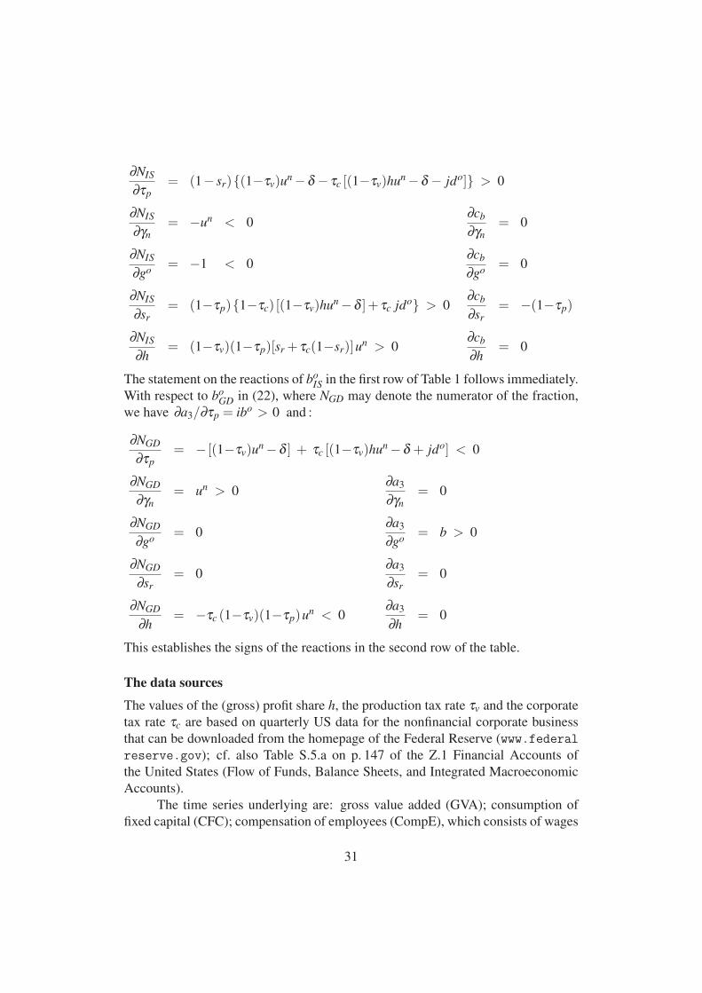
The partial derivatives in eqs in (21), (22) and in Table 1

Let NIS be the numerator of boIS in (21). Then ∂cb/∂τp =−(1− sr) < 0 and :

30

∂NIS

∂τp= (1− sr){(1−τv)u

n−δ − τc [(1−τv)hun−δ − jdo]} > 0

∂NIS

∂γn= −un < 0

∂cb

∂γn= 0

∂NIS

∂go= −1 < 0

∂cb

∂go= 0

∂NIS

∂sr= (1−τp){1−τc) [(1−τv)hun−δ ]+ τc jdo} > 0

∂cb

∂sr= −(1−τp)

∂NIS

∂h= (1−τv)(1−τp)[sr + τc(1−sr)]u

n > 0∂cb

∂h= 0

The statement on the reactions of boIS in the first row of Table 1 follows immediately.

With respect to boGD in (22), where NGD may denote the numerator of the fraction,

we have ∂a3/∂τp = ibo > 0 and :

∂NGD

∂τp= − [(1−τv)u

n−δ ] + τc [(1−τv)hun−δ + jdo] < 0

∂NGD

∂γn= un > 0

∂a3

∂γn= 0

∂NGD

∂go= 0

∂a3

∂go= b > 0

∂NGD

∂sr= 0

∂a3

∂sr= 0

∂NGD

∂h= −τc (1−τv)(1−τp)un < 0

∂a3

∂h= 0

This establishes the signs of the reactions in the second row of the table.

The data sources

The values of the (gross) profit share h, the production tax rate τv and the corporate

tax rate τc are based on quarterly US data for the nonfinancial corporate business

that can be downloaded from the homepage of the Federal Reserve (www.federal

reserve.gov); cf. also Table S.5.a on p. 147 of the Z.1 Financial Accounts of

the United States (Flow of Funds, Balance Sheets, and Integrated Macroeconomic

Accounts).

The time series underlying are: gross value added (GVA); consumption of

fixed capital (CFC); compensation of employees (CompE), which consists of wages

31

& salaries and the employers’ social contributions; the taxes on production and

imports less subsidies (TaxP); the taxes on corporate income (TaxCI), which more

precisely are called current taxes on income, wealth, etc. (paid); the rents paid

(Rent); and the net interest payments (Int), i.e. interest paid minus interest received.

From them we obtain:

τv = TaxP/GVA

h = (GVA − TaxP − CompE)/(GVA − TaxP)

τc = TaxCI/(GVA − TaxP − CompE − CFC − Rent − Int)

(the denominator of τc represents the net profits of the firms, i.e. the operating

surplus net of depreciation and interest and similar payments).

A major alternative data source is the database fmdata.dat in the zip file

fmfp.zip that is provided by Ray Fair on his homepage for working with his

macroeconometric model, on http://fairmodel.econ.yale.edu/fp/fp.htm .

This is a huge plain text file from which the single time series have to be extracted

for further use. Each of them is identified by an acronym. They are explained in

Chapter 6.5, table A2, of the script Macroeconometric Modeling by R.C. Fair, No-

vember 11, 2011, which can be downloaded from http://fairmodel.econ.yale.

edu/mmm2./mm.pdf (last accessed July 2015, though the data we used are of an

older vintage).

It is particularly convenient that the database contains a quarterly series of the

real capital stock (acronym KK) of (essentially) the nonfinancial corporate business

(NFCB). Using the perpetual inventory method, it is based on fixed nonresiden-

tial investment of this sector, and not total fixed nonresidential investment in the

economy, which is on average 1/0.887 = 1.127 times higher (see pp. 184f of the

aforementioned book).

One can then readily compute the time averages of the (annualized) growth

rate of this capital stock and the ratio of the real output over the real capital stock.24

The inflation rate π is obtained from the price deflator of the NFCB output, while

the bond rate i in Table 2 is the three-month treasure bill rate. Regarding the rate

of depreciation, the database gives us an average of 6.62%. This may appear unfa-

miliarly low.25 The Fed data actually yields an average ratio CFC/GVA = 13.21%,

so that multiplying it by our value 0.90 for the output-capital ratio leads to a depre-

ciation rate in the range of 11.90%. Thus we choose to settle down on δ = 10%

(though not very much will depend on this).

24One should better not use the nominal magnitudes in this ratio because the price deflators of

output and capital show different tendencies.25It was steadily increasing from 4.59% in 1983 to 9.41% in 2007.

32

The value for the loan rate j is lastly derived from the US bank prime loan–

middle rate (which is on short-term business loans). It was obtained from Data-

stream, code FRBKPRM.

Calibrating countercyclical government spending

There is in fact certain empirical evidence that government spending is counter-

cyclical. Most conveniently, for the the period 1970 – 1995 we can directly refer

to Fiorito (1997, Table 9 on p. 42), who computes a contemporaneous cross corre-

lation of −0.40 and of −0.47 at a lag of one quarter. Hence, if anything, positive

values may be chosen for the spending coefficient γc in (14). Regarding specific

numerical values one may proceed as follows.

(i) Given a value of γc, simulate a cyclical variant of the model (possibly again

derived from exogenous oscillations of the capital growth rate as in Section

7).

(ii) Construct the time series of the levels of government spending pG from the

variables in intensive form.

(iii) Detrend the series by Hodrick-Prescott and compute the standard deviation

of the cyclical component.

(iv) Compute the same statistic from the empirical data; an immediate reference

could be Table 7 in Fiorito (1997, p. 37), where percentage values between

1.20 and 1.30 are reported.

(v) The deviations of the model-generated from the empirical standard deviations

can be treated as an additional moment and included in the loss function. It

is then to be minimized under suitable variations of γc (and perhaps other

parameters).

References

Bhaduri, A. and Marglin, S. (1990): Unemployment and the real wage: the eco-

nomic basis for contesting political ideologies. Cambridge Journal of Eco-

nomics, 14, 375–393.

Blinder, A.S. and Solow, R.M. (1973): Does fiscal policy matter? Journal of Pub-

lic Economics, 2, 319–337. Reprinted in T.M. Havrilesky and J.T. Boorman

(eds): Current Issues in Monetary Theory and Policy. Arlington Heights

(Ill.): AHM Publishing Corp.; pp. 112–127.

33

Chiarella, C., Flaschel, P. and Franke, R. (2005): Foundations for a Disequilibrium

Theory of the Business Cycle: Qualitative Analysis and Quantitative Assess-

ment. Cambridge: Cambridge University Press 2005.

Dallery, T. (2007): Kaleckian models of growth and distribution revisited: Evaluat-

ing their relevance through simulation. Paper presented at the 11th workshop

of the Research Network Macroeconomic Policies, Berlin, October 2007.

Dutt, A. K. (1984): Stagnation, income distribution and monopoly power. Cam-

bridge Journal of Economics, 8, 25–40.

Fiorito, R. (1997): Stylized facts of government finance in the G-7. IMF Working

Paper 97/142.

Flaschel, P., Franke, R. and Semmler, W. (1997): Dynamic Macroeconomics: Insta-

bility, Fluctuations, and Growth in Monetary Economies. Cambridge, Mass:

MIT Press.

Franke, R. (2009): Applying the method of simulated moments to estimate a small

agent-based asset pricing model. Journal of Empirical Finance, 16, 804–815.

Franke, R., Jang, T. and Sacht, S. (2015): Moment matching versus Bayesian es-

timation: Backward-looking behaviour in a New-Keynesian baseline model.

North American Journal of Economics and Finance, 31 (2015), 126–154.

Franke, R. and Yanovski, B. (2015): On the long-run equilibrium value of Tobin’s

average Q. European Journal of Economics and Economic Policies: Inter-

vention (forthcoming).

Hein, E. and Schoder, C. (2011): Interest rates, distribution and capital accumula-

tion—A post-Kaleckian perspective on the US and Germany. International

Review of Applied Economics, 25, 693–723.

Jang, T. and Sacht, S. (2015): Animal spirits and the business cycle: Empirical

evidence from moment matching. Metroeconomica (in press).

Lavoie, M. (2014): Post-Keynesian Economics: New Foundations. Cheltenham,

UK: Edward Elgar.

Lavoie, M. (2010): Surveying short-run and long-run stability issues with the Ka-

leckian model of growth. In M. Setterfield (ed.), Handbook of Alternative

Theories of Economic Growth. Cheltenham, UK: Edward Elgar; pp. 132–

156.

Lee, B.-S. and Ingram, B.F. (1991): Simulation estimation of time series models.

Journal of Econometrics, 47, 197–205.

34

Lerner, A.P. (1943): Functional finance and the federal debt. Social Research, 10,

38–57.

Lojak, B. (2014): Investor sentiment, corporate debt and inflation in a feedback-

guided model of the business cycle. Master thesis, University of Kiel.

Nikolaidi, M. (2014): Margins of safety and instability in a macrodynamic model

with Minskyan insights. Structural Change and Economic Dynamics, 31,

1–16.

Rowthorn, B. (1981): Demand, real wages and economic growth. Thames Papers

in Political Economy, Autumn, pp. 1–39.

Ryoo, S. and Skott, P. (2015): Fiscal and monetary policy rules in an unstable econ-

omy. Working paper, Adelphi University and University of Massachusetts.

Ryoo, S. and Skott, P. (2013): Public debt and full employment in a stock-flow con-

sistent model of a corporate economy. Journal of Post Keynesian Economics,

35, 511–527.

Schoder, C. (2014): Instability, stationary utilization and effective demand: A struc-

turalist model of endogenous cycles. Structural Change and Economic Dy-

namics, 30, 10–29.

Skott, P. (2012): Theoretical and empirical shortcomings of the Kaleckian invest-

ment function. Metroeconomica, 63:1, 109–138.

Skott, P. (2010): Growth, instability and cycles: Harrodian and Kaleckian models

of accumulation and income distribution. In M. Setterfield (ed.), Handbook of

Alternative Theories of Economic Growth. Cheltenham, UK: Edward Elgar;

pp. 108–131.

Skott, P. (1989): Conflict and Effective Demand in Economic Growth. Cambridge,

UK: Cambridge University Press.

Skott, P. and Ryoo, S. (2008): Macroeconomic implications of financialisation.

Cambridge Journal of Economics, 32, 827–862.

Steindl, J. (1952): Maturity and Stagnation in American Capitalism. Oxford: Basil

Blackwell.

35