Juha Kännö

A short-term price forecast model for theNordic electricity markets

School of Science

Thesis submitted for examination for the degree of Master ofScience in Technology.

Espoo 23.4.2013

Thesis supervisor:

Prof. Ahti Salo

Thesis instructor:

M.Sc. (Econ.) Henri Äijö

A’’ Aalto UniversitySchool of Science

aalto universityschool of science

abstract of themaster’s thesis

Author: Juha Kännö

Title: A short-term price forecast model for the Nordic electricity markets

Date: 23.4.2013 Language: English Number of pages: 59

Department of Mathematics and Systems Analysis

Professorship: Applied mathematics Code: Mat-2

Supervisor: Prof. Ahti Salo

Instructor: M.Sc. (Econ.) Henri Äijö

The Nordic countries have a common wholesale electricity market, where the priceof electricity is determined by principles of supply and demand. The electricityexchange, Nord Pool Spot, calculates each day wholesale, or spot prices for eachhour of the day ahead. Price forecasts are used by electricity producers and largeconsumers to support operational planning and trading decisions.

Short-term price forecasting typically aims at predicting spot prices up to twoweeks ahead. Many existing short-term forecasting approaches are based on time-series methods. They are appealing, because forecasting requires at minimum onlyhistorical price data, and the model specification does not heavily rely on the struc-ture of the underlying market. However, the utilization of both external variablesand structural information could increase the transparency of the forecasting pro-cess and enable the analysis of different scenarios.

This thesis presents the main elements of the Nordic electricity market and re-views prior research on electricity price forecasting models. Based on the findings,a framework for short-term price forecasting is proposed. Price is modelled bycombining an external demand estimate with supply functions. A heuristic algo-rithm is developed for the estimation of supply functions from historical marketdata, and an attempt is made to explain changes in the pricing of supply by funda-mental drivers. The implementation of the framework is tested against historicalmarket data from years 2009–2011.

Hourly spot prices can be represented by the proposed framework under mostcircumstances. Temporal shifts of supply functions representing particular dayscan be used to analyse the effects of market fundamentals on pricing. It was foundthat the effects of fundamentals are highly dynamic and challenging to quantify.

Keywords: electricity markets, spot price, forecasting,fundamental models, supply function

aalto-yliopistoperustieteiden korkeakoulu

diplomityöntiivistelmä

Tekijä: Juha Kännö

Työn nimi: Sähkön hinnan ennustaminen lyhyellä aikavälillä pohjoismaisillasähkömarkkinoilla

Päivämäärä: 23.4.2013 Kieli: Englanti Sivumäärä: 59

Matematiikan ja systeemianalyysin laitos

Professuuri: Sovellettu matematiikka Koodi: Mat-2Valvoja: Prof. Ahti Salo

Ohjaaja: KTM Henri Äijö

Pohjoismailla on yhteiset sähkön tukkumarkkinat, joilla sähkön hinta määräytyykysynnän ja tarjonnan mukaan. Sähköpörssi Nord Pool Spot laskee päivittäinsähkön tukkuhinnat eli niin sanotut spot-hinnat seuraavan vuorokauden jokaiselletunnille. Sähköntuottajat ja -kuluttajat tarvitsevat hintaennusteita operatiivisensuunnittelun ja pörssikaupankäynnin tueksi.

Lyhyen aikavälin ennustusmallien tavoitteena on tyypillisesti ennustaa tuntikoh-taiset spot-hinnat kahden viikon päähän. Lyhyellä aikavälillä spot-hintoja ennus-tetaan usein aikasarjamalleilla. Ne ovat houkuttelevia, koska syötteeksi riittäävähimmillään historiallinen hintadata, eikä mallin määrittely riipu vahvasti allaolevan markkinan rakenteesta. Hyödyntämällä sekä ulkoisia muuttujia että ra-kenneinformaatiota voidaan ennustamisesta tehdä läpinäkyvämpää ja analysoidaerilaisia skenaarioita.

Tässä diplomityössä tarkastellaan pohjoismaisten sähkömarkkinoiden peruspiir-teitä ja aikaisempaa hinnan ennustamiseen liittyvää tutkimusta. Tähän perustuenesitetään malli, jossa spot-hinta lasketaan yhdistämällä ulkoinen kysyntäennus-te tarjontafunktioihin. Työssä kehitetään heuristinen algoritmi tarjontafunktioi-den estimointiin markkinadatasta. Lisäksi työssä tutkitaan tarjonnan hinnoittelunriippuvuutta markkinafundamenteista. Mallia testataan markkinadatalla vuosilta2009–2011.

Mallilla pystytään kuvaamaan tuntitason spot-hintoja useimmissa tilanteissa.Päiväkohtaisten tarjontafunktioiden muutoksia vertailemalla voidaan analysoi-da markkinafundamenttien vaikutusta hinnoitteluun. Fundamenttien vaikutuksetovat hyvin dynaamisia ja niiden kvantifiointi on haasteellista.

Avainsanat: sähkömarkkinat, spot-hinta, ennustaminen,fundamenttipohjaiset mallit, tarjontafunktio

iv

Acknowledgements

The completion of this thesis would not have come about without the help andsupport of several people, to say nothing of the innumerable cups of coffee whichfuelled the train of thought.

The thesis was written as an assignment from UPM. First I wish to thank ChristianHoffmann, Director of Energy Market Analysis, for entrusting me with the oppor-tunity to work on this topic. I am grateful to my instructor Henri Äijö, who helpedme to develop an understanding of the fundamentals of electricity markets. I wouldalso like to extend my appreciation to the members of the project steering group. Iam indebted to Timo Javanainen for subtle guidance and many encouraging discus-sions, Anne Särkilahti for perceptive comments and Ljubov Fedetskina for feedbackin application development. Moreover, special thanks go out to Lari Järvenpää forthe great company to toss ideas around. All colleagues, with whom I have had thepleasure to work with, have my sincere gratitude for their time and support.

I want to thank my supervisor, Professor Ahti Salo, for guidance in the thesis devel-opment and insightful teaching, which has cultivated my understanding of systemsanalysis and its application to actual business cases. I am also grateful to Dr. AfzalSiddiqui for suggestions that helped me to improve the thesis towards the end ofthe writing.

I would like to express my appreciation to the friends who have accompanied meon the road to graduation. It would overshadow the length of the actual thesis tomention individually and equally each wonderful person who deserves it. However,it is thanks to all of you that I have grown to be the person that I am now.

Finally, I want to thank my family for their love, care and support.

Helsinki 28.4.2013

Juha Kännö

Contents

1 Introduction 11.1 Background and motivation . . . . . . . . . . . . . . . . . . . . . . . 11.2 Research objectives . . . . . . . . . . . . . . . . . . . . . . . . . . . . 31.3 Structure of the thesis . . . . . . . . . . . . . . . . . . . . . . . . . . 3

2 The Nordic electricity market 52.1 Consumption . . . . . . . . . . . . . . . . . . . . . . . . . . . . . . . 52.2 Generation . . . . . . . . . . . . . . . . . . . . . . . . . . . . . . . . . 7

2.2.1 Conventional thermal generation . . . . . . . . . . . . . . . . 72.2.2 Nuclear power . . . . . . . . . . . . . . . . . . . . . . . . . . . 82.2.3 Wind power . . . . . . . . . . . . . . . . . . . . . . . . . . . . 92.2.4 Hydro power . . . . . . . . . . . . . . . . . . . . . . . . . . . 92.2.5 Optimal generation mix . . . . . . . . . . . . . . . . . . . . . 9

2.3 Power grid . . . . . . . . . . . . . . . . . . . . . . . . . . . . . . . . . 112.4 Electricity trading . . . . . . . . . . . . . . . . . . . . . . . . . . . . . 13

2.4.1 Physical market . . . . . . . . . . . . . . . . . . . . . . . . . . 132.4.2 Financial market . . . . . . . . . . . . . . . . . . . . . . . . . 15

2.5 Generation scheduling and pricing . . . . . . . . . . . . . . . . . . . . 162.6 Fundamentals and characteristics of electricity prices . . . . . . . . . 18

3 Literature on electricity price models 223.1 Cost-based models . . . . . . . . . . . . . . . . . . . . . . . . . . . . 223.2 Game-theoretic models . . . . . . . . . . . . . . . . . . . . . . . . . . 233.3 Stochastic models . . . . . . . . . . . . . . . . . . . . . . . . . . . . . 243.4 Autoregressive models . . . . . . . . . . . . . . . . . . . . . . . . . . 253.5 Artificial intelligence-based models . . . . . . . . . . . . . . . . . . . 263.6 Fundamental models . . . . . . . . . . . . . . . . . . . . . . . . . . . 27

4 An approach to short-term spot price forecasting 294.1 Proposed framework and key assumptions . . . . . . . . . . . . . . . 29

4.1.1 Choice of approach . . . . . . . . . . . . . . . . . . . . . . . . 294.1.2 Key assumptions . . . . . . . . . . . . . . . . . . . . . . . . . 324.1.3 Specification of the framework . . . . . . . . . . . . . . . . . . 33

4.2 Description of data . . . . . . . . . . . . . . . . . . . . . . . . . . . . 354.2.1 Data set . . . . . . . . . . . . . . . . . . . . . . . . . . . . . . 35

v

vi

4.2.2 Fundamental drivers of supply . . . . . . . . . . . . . . . . . . 364.3 Validation of the framework . . . . . . . . . . . . . . . . . . . . . . . 42

4.3.1 Estimating the supply function . . . . . . . . . . . . . . . . . 424.3.2 Forecasting with a static supply function . . . . . . . . . . . . 444.3.3 Analysing the effects of changing fundamentals . . . . . . . . 48

4.4 Facilitating price forecasts in practice . . . . . . . . . . . . . . . . . . 50

5 Conclusions 52

Bibliography 55

Symbols and abbreviations

Symbols

Calculation of short-run marginal cost

cfuel Cost of fuelcCO2 Cost of emission allowancekF X Currency exchange ratekHV Heat value of fuelkeff Efficiency rate of power plantkCO2 Emission factor of power plant

Hydro reservoir equations

Rt Reservoir level at the end of period tRt Upper reservoir levelRt Lower reservoir levelwt Inflow into the reservoir in period teH

t Water released from the reservoir in period t

Supply function estimation algorithm

ti Timeqi Quantitypi Pricexi = {ti, qi, pi} Observation of supply dataX = {xi} Set of supply data observationsXSupplyF unction Set of data points that define the estimated supply functionvint Volume interval parameter of the estimation algorithm

vii

viii

Fundamental regression models

h Hourd Dayfd,h Actual value of a fundamentalf Base value of a fundamentalxd,h Value of the fundamental predictor variablepd,h Priceqd,h Demand volumeβi Regression coefficientsεd,h Error term

Abbreviations

ANN Artificial neural networkARIMA Autoregressive integrated moving average (time-series model)CCGT Combined cycle gas turbineCET Central European TimeCfD Contract for differenceCHP Combined heat and powerEMPS EFI’s Multi-area Power-market SimulatorMWhe Megawatt-hour of electricityMWhth Megawatt-hour of thermal energyPDP Price-dependent productionPIP Price-independent productionSFE Supply function equilibriumSRMC Short-run marginal costTSO Transmission system operatorUMM Urgent market message

Chapter 1

Introduction

1.1 Background and motivation

With the liberalization of electricity markets, power has become a tradable com-modity. As a consequence, formerly regulated electricity tariffs have made way formarket-based price determination (Nord Pool Spot, 2011b). Electricity differs in-herently from other goods in that it cannot be stored. Hence, the amount of powerfed into the grid must constantly match consumption to ensure the stability of thepower system. In addition, the transmission of electricity requires an extensive in-frastructure. These facts are essential to the nature of the power market (see e.g.Weron, 2007).

Deregulation of the Nordic market started in Norway in the early 1990s (Flatabøet al., 2003). Today Norway, Sweden, Finland, Denmark and Estonia form a singlemarket, where electricity is traded in a common power exchange operated by NordPool Spot AS (Nord Pool Spot, 2011b). Its main market place is the day-aheadauction market Elspot, which determines the spot price. According to Nord PoolSpot (2011b), the power exchange serves the society first by providing transparentpricing for wholesale electricity trade. Second, the spot price is used as referenceprice in the electricity derivatives market, and quotes for long-term contracts reflectthe expectations for future electricity prices. Third, the market provides a systemfor maintaining a balance between physical supply and demand.

Producers, retailers, and traders, as well as big end-users of electricity, participatein the day-ahead market. Participants submit bids, which express combinations of

1

2

how much energy they are willing to buy or sell at a particular price, for each hourof the following day. After the closing of the bidding period, all bids are fed intothe price determination mechanism. Sell offers are accepted in increasing price orderand buy offers in decreasing price order, until an equilibrium price and volume aremet (Nord Pool Spot, 2011c). Producers with flexible generation assets can use adetailed price forecast for price-setting purposes, or to optimize their productionschedule in order to maximize profits (Bunn, 2000).

Price forecasting activities can be classified by the time horizon, resolution, andpurpose of use (Weron and Misiorek, 2006). It is conventional to talk about long-term, medium-term and short-term price forecasting. Long-term price forecastingsupports strategic decisions, such as investments in new power plants, and has typ-ically a time horizon of several years. Medium-term price forecasting is used forbalance sheet forecasts and risk management, and typically produces a probabil-ity distribution of estimated prices (e.g. Eydeland and Wolyniec, 2003; Bunn andKarakatsani, 2003). The granularity of medium and long-term forecasts spans fromweeks to years. Short-term forecasting, on the other hand, attempts to predict actualprices in the day-ahead market. In the case of the Nordic market, the main interestlies in forecasting hourly prices from the following day up to one or two weeks ahead.

Short-term forecasting is challenging due to the complexity of the market. Theprice of electricity is related to external factors referred to as market fundamentals.Even though it is known that—for instance—fuel prices, temperatures, precipitation,and electricity prices of neighbouring markets affect the Nordic prices (e.g. Kalatie,2005; Vehviläinen and Pyykkönen, 2005; Johnsen, 2001), quantifying their joint effecton the price is difficult. Moreover, human psychology induces seemingly irrationalmarket behaviour (Jabłonska, 2011).

A great deal of research has concentrated on modelling spot prices with time seriesmodels (e.g. Nogales et al., 2002; Guthrie and Videbeck, 2007), whose performancecan be improved by incorporating fundamental external variables (e.g. Weron andMisiorek, 2008; Jónsson, 2008) or regime-switching properties (e.g. Karakatsani andBunn, 2008b). Another line of research is based on artificial neural networks (ANN),which are good at capturing complex and non-linear effects (e.g. Gao et al., 2000;Catalão et al., 2007; Livanis and Zapranis, 2007). These approaches can be char-acterized as ‘black-box’, as they do not represent the structure of the underlyingmarket. Because these models do not answer to the question, through which mech-anism changes in market fundamentals affect the spot price, they have a limited

3

value in the analysis of different fundamental scenarios. Short-term forecasting callsfor more transparent approaches. This thesis investigates the usability of a ‘grey-box’ approach, which incorporates knowledge about the structure of the electricitymarket into the model itself, and could thus improve the credibility and accuracy ofthe model.

1.2 Research objectives

The purpose of this thesis is to develop and evaluate a model for forecasting thehourly prices in Nord Pool Spot’s day-ahead market one week ahead. The model isintended to support support operational planning and trading decisions. From thisbasis the objectives of the thesis are to

1. identify and analyse key factors in spot price formation

2. develop a modelling framework for forecasting hourly prices

3. implement a forecasting model based on the framework.

Electricity prices are characterized by a periodic profile, spikes and a tendency torevert to a mean level (e.g. Bunn and Karakatsani, 2003; Weron, 2005; Meyer-Brandis and Tankov, 2008). Considering the model’s intended purpose of use, thedesign should provide accurate estimates both in terms of hourly profile and pricelevel, and enable sensitivity analysis with respect to market fundamentals.

The scope of this thesis is limited to the system price, which is calculated withoutsetting constraints on the transmission capacities between different zones in the mar-ket (Nord Pool Spot, 2011b). In the case that transmission lines are congested, therewill be different prices in the affected zones, or so-called bidding areas. Modellingthe area prices adds an extra layer of complexity, which constitutes an interestingtopic for further studies.

1.3 Structure of the thesis

The remainder of this thesis is organized as follows. Chapter 2 introduces the mainelements of the Nordic power market. Chapter 3 reviews prior research on electricityprice modelling and forecasting. Emphasis is put on short-term methods, but other

4

approaches are also presented briefly to provide a general view of the field. Chap-ter 4 proposes a short-term spot price forecasting framework, which is validatedagainst historical market data. The analysis focuses particularly on the effects ofmarket fundamentals and their implications on practical forecasting activities. Fi-nally, Chapter 5 presents the conclusions of the research.

Chapter 2

The Nordic electricity market

2.1 Consumption

Electricity consumption in the Nordic countries is mainly made up by electricity-intensive industries and direct electricity heating (NordREG, 2012). Largest sourcesof consumption vary by country, but generally follow temperature variations andeconomic growth. In 2010, the total electrical energy consumption of Norway, Swe-den, Finland and Denmark amounted to 361 TWh (Eurostat, 2012). Industrial usehad a 41 % share of total consumption. Paper and pulp are the most consumingindustrial sector in Finland and Sweden, while metal and petrochemical industriesare the biggest consumers in Norway. Denmark has considerably lower industrialconsumption. In total, residential consumption amounted to 31 % of the total con-sumption, while the share of services was 25 %. The price-elasticity of consumptionis very low in the short run (Bye and Hansen, 2008), and found to increase alongwith the spot price (Johnsen, 2001).

Consumption exhibits strong periodical patterns, which are illustrated in Figure 2.1.First, there is a seasonal trend which follows the temperature due to the widespreaduse of electrical heating. Second, consumption is lower in the weekends than duringworking days, because many businesses are inactive during weekends. A similar effectcan be observed on public holidays. Third, there is a strong intra-day profile. Themorning peak occurs when people arrive to their working places, and the eveningpeak is related to increased household consumption when people come home fromwork (NordREG, 2012).

5

6

Q1−09 Q2−09 Q3−09 Q4−09 Q1−10 Q2−10 Q3−10 Q4−10 Q1−11 Q2−11 Q3−11 Q4−11

0

5000

10000

15000Seasonal profile

Con

sum

ptio

n (G

Wh/

wee

k)

Q1−09 Q2−09 Q3−09 Q4−09 Q1−10 Q2−10 Q3−10 Q4−10 Q1−11 Q2−11 Q3−11 Q4−11

−20

0

20

40

Tem

pera

ture

(C

elci

us)

Consumption (weekly)Average temperature (Norway & Sweden)

21.02.11 22.02.11 23.02.11 24.02.11 25.02.11 26.02.11 27.02.11 28.02.11

45

50

55

60

65

70Typical weekly and intra−day profiles (21.02.−28.02.2011)

Con

sum

ptio

n (G

Wh/

hour

)

Consumption (hourly)

Figure 2.1: Seasonal, weekly, and intra-day profiles of electricity consumption

7

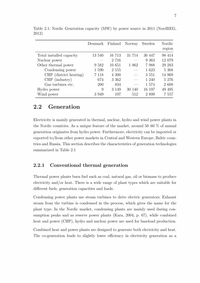
Table 2.1: Nordic Generation capacity (MW) by power source in 2011 (NordREG,2012)

Denmark Finland Norway Sweden Nordicregion

Total installed capacity 13 540 16 713 31 714 36 447 98 414Nuclear power — 2 716 — 9 363 12 079Other thermal power 9 582 10 651 1 062 7 988 29 283

Condensing power 1 590 2 155 — 1 623 5 368CHP (district heating) 7 118 4 300 — 3 551 14 969CHP (industry) 674 3 362 — 1 240 5 276Gas turbines etc. 200 834 — 1 574 2 608

Hydro power 9 3 149 30 140 16 197 49 495Wind power 3 949 197 512 2 899 7 557

2.2 Generation

Electricity is mainly generated in thermal, nuclear, hydro and wind power plants inthe Nordic countries. As a unique feature of the market, around 50–60 % of annualgeneration originates from hydro power. Furthermore, electricity can be imported orexported to/from other power markets in Central and Western Europe, Baltic coun-tries and Russia. This section describes the characteristics of generation technologiessummarized in Table 2.1

2.2.1 Conventional thermal generation

Thermal power plants burn fuel such as coal, natural gas, oil or biomass to produceelectricity and/or heat. There is a wide range of plant types which are suitable fordifferent fuels, generation capacities and loads.

Condensing power plants use steam turbines to drive electric generators. Exhauststeam from the turbine is condensed in the process, which gives the name for theplant type. In the Nordic market, condensing plants are mainly used during con-sumption peaks and as reserve power plants (Kara, 2004, p. 67), while combinedheat and power (CHP), hydro and nuclear power are used for baseload production.

Combined heat and power plants are designed to generate both electricity and heat.The co-generation leads to slightly lower efficiency in electricity generation as a

8

trade-off to heat generation. Total efficiency in terms of electricity and heat genera-tion is generally higher than with a condensing power plant. Industrial CHP plantsare used to produce steam for heat-requiring processes in pulp and paper mills, andin other industries. CHP plants are also used for district heating in urban areas.The ratio of electricity and heat output depends on the plant design. To operateeconomically, a CHP plant requires a stable and adequate heat load. It suits wellfor the Nordic climate with long cold periods, when the demand both for electricityand heat is high (Kara, 2004, p. 75).

In combined-cycle gas turbine (CCGT) technology, a gas-fired combustion turbinedrives the electric generator. The heat of gas turbine’s exhaust, which otherwisewould be wasted, is used to generate steam that drives another generator. CCGTplants producing both electricity and heat can reach efficiency rates of over 90 %.

Gas turbines and diesel engines can be brought on-line very fast, and are typicallyused for peak power or reserve power.

The short-run marginal cost (SRMC) of thermal generation typically used to deter-mine, whether it is profitable to operate a condensing plant in the short run. It isdefined as

SRMC [EUR/MWhe] = cfuel · kF X · k−1HV · k−1

eff + cCO2 · kCO2 · k−1eff ,

where cfuel [USD/t] is the cost of fuel, kF X [EUR/USD] the exchange rate,kHV [MWhth/t] the heat value of fuel, keff [MWhe/MWhth] the efficiency rateof the power plant, cCO2 [EUR/tCO2 ] the cost of emission allowance and kCO2

[tCO2/MWhth] the emission factor. MWhth and MWhe stand for MWh of thermalenergy and electricity, respectively. Condensing plants have also notable start-upcosts arising mainly from fuel that must be burned in order to bring the plant upto running state (e.g. Førsund, 2007, pp. 116–117). These costs are substantial andmust be also taken into account in operating decisions.

2.2.2 Nuclear power

Nuclear power plants use the energy of fission reaction to boil water, but operateotherwise with same principle as condensing power plants. In Finland and Sweden,nuclear power is used for baseload production. Nuclear plants typically have a veryhigh operating rate.

9

2.2.3 Wind power

Wind power plants use the kinetic energy of wind to drive an electric generator.Wind power’s most significant characteristic is its volatility: the output dependson actual wind speed. A power system cannot thus be built on wind power only.Denmark is world leader with a 21 % share of wind power in its electricity supply(World Wind Energy Association, 2011).

2.2.4 Hydro power

Hydro power plants use the potential energy of water to drive water turbines con-nected to electric generators. Plants can be characterised by how well productioncan be regulated. Generation of run-of-river plants depends on the natural flow inthe waterway where the plant is located. Dams can be used to store some water,which gives better control over the production. A reservoir plant maintains a largewater storage, where water can accumulate. The size of a reservoir can be equal evenup to the production volume of several years. Water is typically discharged throughplant’s turbines, but it can be also directed to spillways leading it past the plant.

Javanainen (2005) notes that the climate and geography in Norway are very suit-able for reservoir hydro power production, whereas Finnish and Swedish hydro powerplants have less storage capacity, and are thus more dependent on the natural flows.Figure 2.2 compares weekly inflows and hydro production volumes in Norway andSweden. It appears that the production volumes in Sweden are more strongly con-nected to inflows, which supports the argument.

Inflow is a measure of water entering the water system, where a plant is located. Itsmain factors are precipitation and melting snow. Inflow corresponds to an increasein the reservoir level, whereas a discharge decreases it. Hydro balance measures thedeviation of current water resources to a multi-year average value of that time of theyear. In addition to the reservoir content, hydro balance takes into account watercontained in the soil and snow which will affect the reservoir.

2.2.5 Optimal generation mix

The load-duration curve, illustrated by Figure 2.3, can be used to determine an op-timal mix of generation technologies that are used to satisfy the electricity demand.

10

2009 2010 2011

1000

2000

3000

4000Norway

Pro

duct

ion

(GW

h/w

eek)

2009 2010 2011

0

500

1000

1500

Inflo

w (

GW

h/w

eek)

Hydro productionInflow

2009 2010 2011

500

1000

1500

2000Sweden

Pro

duct

ion

(GW

h/w

eek)

2009 2010 2011

0

500

1000

1500

Inflo

w (

GW

h/w

eek)

Hydro productionInflow

Figure 2.2: Inflow and hydro power production in Norway and Sweden. The timingof inflows correlates between the countries, but Swedish production volumes appearto be more strongly connected to arriving inflows.

The choice of technology depends on the amount of power required and the expectedannual operating hours for different load levels. It is economically reasonable to coverbaseload with technologies which have low variable costs, while considerable fixedcosts will then be distributed to a large number of operating hours. On the otherhand, peak load plants and power reserves, which are activated in extreme situa-tions, are typically based on technologies with low fixed costs and higher variablecosts, because the fixed costs must be recovered during few annual operating hours.(Vuorinen, 2009)

In the Nordic countries, highest precedence is given to production forms that cannot

11

1000 2000 3000 4000 5000 6000 7000 8000 8760

20

25

30

35

40

45

50

55

60

65

70Nordic load−duration curves

Hours

Load

(G

W)

200920102011

Figure 2.3: Nordic load-duration curves

be regulated, that are wind and a part of hydro power. They are followed by otherproduction forms in an increasing order of marginal production costs, or the so-called merit order, as illustrated in Figure 2.4. In addition to wind and unregulatedhydro power, baseload production consists of nuclear power and electricity fromCHP production. They are followed by condensing power plants, and finally gasturbines and other peak-load plants.

In a perfectly competitive market, the market price will equal the marginal produc-tion cost of the most expensive generator that is dispatched. Regulated hydro poweris somewhat special in the generation mix: It has extremely low marginal costs, andgeneration can normally be scaled with high flexibility. Consequently, regulated hy-dro power is allocated to periods of high demand, when its opportunity cost is high.In the absence of hydro power generation, expensive generators would have to bedispatched in the merit order.

2.3 Power grid

This section outlines the structure and operation of the Nordic power grid. The gridcan be broken down to national main grids, regional transmission networks and localdistribution networks. Transmission lines between main grids connect the power

12

Coal condensing

Gas CCGT

Gas turbine

Wind, solar RoR hydro

Nuclear

CHP

Baseload (price-independent production) Price-dependent production

Peak reserves

Cumulative volume (MWh/h)

Sh

ort

-run

ma

rgin

al c

ost

(EU

R/M

Wh)

Reservoir hydropower

Demand

Figure 2.4: Idealised merit order curve of Nordic production. It should be notedthat in reality plants using same generation technology can have different marginalproduction costs.

systems of neighbouring countries. The main grids are owned and maintained bynational transmission system operators (TSOs). They are public utilities, which areresponsible for the stability of the power system in their area. The Nordic TSOs areStattnet (Norway), Svenska Kraftnät (Sweden), Fingrid (Finland) and Energinet.dk(Denmark).

One can picture the Nordic market as a system of water tanks, where the waterflow represents electric power, and pipes connecting the tanks are transmission lines(Figure 2.5). Producers pour power into the system, and consumers tap it. Whenthe water surface stays at a constant level, demand and supply are in balance.Producers and consumers are not geographically evenly distributed. For instance,most hydro power plants are scattered around Norway, and the northern parts ofSweden and Finland. Due to the limited capacity of transmission lines, arbitrarysupply and demand cannot be matched. Instead, local generators will be dispatchedin the vicinity of the consumer.

The market uses bidding areas1 as an economic tool to deal with the transmissionbottlenecks. Each country makes up at least one bidding area, but TSOs may di-vide their country into more areas. Each area has an adequate transmission and

1The term price area used by some sources is interchangeable with bidding area.

13

Producers

End users

50 Hz

Figure 2.5: Depiction of the power system as system of water tanks. When supplyand demand are in balance, the electric current in the grid is at nominal 50 Hzfrequency. Imbalances cause voltage and frequency fluctuations, which endanger thestability of the power system. Source: Nord Pool Spot (2011b)

distribution capacity within itself, but transmission lines between areas can becomecongested. Should it happen that power cannot ‘flow’ between two bidding areas tomatch total supply and demand, Nord Pool Spot increases the electricity price inthe area with a supply deficit by an amount which lowers the demand to match theavailable supply. Consequently, the electricity price in the area with supply surplusenjoys a lower price. Since the beginning of 2012 Norway is divided into five biddingareas, Sweden into four areas and Denmark into two areas. Finland and Estoniamake up their own bidding areas.

2.4 Electricity trading

This section presents the markets where physical electricity and electricity deriva-tives are traded. Trading in the physical market involves always a physical deliveryof power. The physical market covers day-ahead, intra-day and regulating powermarkets. The financial markets deal with electricity derivatives, which are settledby cash payments only and do not involve any physical delivery of electricity.

2.4.1 Physical market

Elspot is the main marketplace in Nord Pool Spot. Approximately 74 % of electricityconsumed in all Nordic countries was traded in the exchange in 2011 (Nord PoolSpot, 2011a). Elspot is a day-ahead market, meaning that every day the powerdelivery for each hour of the following day is subject to trade. Market participantssubmit bids where they state the price and quantity of power which they are willing

14

to sell or buy at every hour. Several price steps can be specified. Elspot is a closedauction, and participants have no knowledge about other’s bids. Bids are submittedeach day until the deadline called gate closure at 12:00 CET.

After gate closure the exchange determines spot prices for each hour. The systemprice is a reference price which does not take into account transmission constraintsbetween bidding areas. If available transmission capacities do not constrain powerdelivery, system price will be the actual price in each bidding area. Otherwise areaprices are calculated so that demand and supply in each bidding area do not violatetransmission constraints. In effect, the area price will be below system price insurplus areas and above it in deficit areas. The prices are normally published between12:30 to 12:45 CET.

Elbas market supplements Elspot by enabling trading up to one hour before thedelivery. There are 12 to 36 hours between gate closure and the delivery hour.Sellers and buyers may need to deviate from the commitments made in Elspot bids.For instance, a drop in temperature could increase demand, or a seller might beunable to produce power due to a plant outage. Elbas quotes the highest buy priceand lowest sell price for each hour, and orders are executed immediately when pricesmatch.

Management of the power balance requires still finer market instruments than Elspotand Elbas markets. For this reason the TSOs run in each country a regulating powermarket, where participants can make offers to adjust their generation or consump-tion capacity within an hour. TSOs can accept these offers in the situation, whereconsumption exceeds generation (known as up-regulation) or generation exceeds con-sumption (down-regulation).

Elspot bid types and the price calculation principle

Willingness to buy or sell power in Elspot can be expressed by different types ofbids. Hourly bid is the most common type. It consists of a set of price limits andcorresponding energy volumes for the applicable delivery hour. An hourly bid mustat least specify volumes for the minimum and maximum price limits set by NordPool Spot. Values between the given price steps are determined by means of linearinterpolation. Flexible hourly bids let a participant to sell, but not to buy, energy inany hour of the trading day. The bid can be activated for one hour of the tradingday. Block bids express willingness to buy or sell power during a minimum time of

15

three consecutive hours. A block bid consists of a price limit, the hourly energyvolume and the start and stop times. (Nord Pool Spot, 2011c)

The objective of Nord Pool Spot’s price calculation algorithm is to maximize totalsocial welfare, which is the sum of consumers’ and producers’ surplus over all hours,bidding areas and bid types. The problem is subject to several constraints, whichensure that (Nord Pool Spot, 2011c)

1. the volume of purchases and power flow in is equal to the volume of sales andpower flow out in each bidding area

2. imports and exports to/from other markets satisfy specified conditions

3. flows between bidding areas do not exceed available transmission capacities

4. flexible hourly bids and block bids are activated only if they increase the totalwelfare.

Following gate closure, the exchange determines the system price and area prices. Inthe system price calculation, aggregated supply and demand curves are constructedfor each hour from the hourly bids of all bidding areas. The intersection of the curvesgives an equilibrium price and turnover. Block bids and flexible hourly bids areactivated if their inclusion improves the value of the objective function. Constraint 3is not used while the system price is calculated. If constraint 3 is binding when in use,bidding areas will have different area prices. In the area price calculation, aggregatedsupply and demand curves are created for each area from the bids of the marketplayers located in that area. If a bidding area has power surplus (extra power flowsto an adjacent area), a volume corresponding to the transmission capacity is addedas price-independent demand to the surplus area. The same volume is added asprice-independent supply to the deficit area.

2.4.2 Financial market

The spot prices are highly volatile due to the instantaneous nature of the market.Market participants, who are directly exposed to the spot price, face a great uncer-tainty about their future income or expenditure. A producer may want to fix thesales price for part of their future production, which secures a certain future cashflow even if the price level would drop. Likewise, a big consumer may want to fixthe purchase price for a certain volume. Products of the financial market are mainly

16

used for protection against the price risk and proprietary trading.

Standardized contracts are traded in an exchange operated by NASDAQ OMX Com-modities. Main products are futures, forwards and options. There are also contractsfor differences (CfDs), which can be used to hedge against the difference betweenthe system price and an area price. Financial contracts do not involve any physicaldelivery of power. They are settled by cash payments which depend on the contractprice and the reference price, which is the system price (or in case of CfD, the dif-ference of system and area price) at the time of delivery. Trading financial contractsoutside of the exchange is called the over-the-counter market. There parties can en-ter into any type of contracts desired. A bilateral power contract can for examplecouple price with outside temperature.

The time horizon in the financial market is six years ahead. Within the horizon,futures are available for delivery periods of days and weeks, and forwards for months,quarters and years. A forward curve quotes the prices of contracts with differentmaturities and thus tells how the market values electricity that will be delivered inthe future. Sometimes the forward price includes a risk premium and may thus bevery different than a spot price forecast.

2.5 Generation scheduling and pricing

This section discusses generation scheduling activities in a deregulated market, suchas the Nordic market, with both hydro and thermal generation capacity. The task offinding an optimal generation schedule is closely related to electricity price forecast-ing. Depending on the type of scheduling approach, price can be endogenous to themodel, or come from an external price forecasting model. This section introducesthe concept of water value, which will play an important role in the forecastingframework proposed in this thesis.

In regulated markets, the objective of generation scheduling for a utility was to mini-mize overall costs while satisfying the demand in their concessionary area (Wolfganget al., 2009). The utilities were also collectively responsible for maintaining powerreserves, which were required to ensure the stability of the system. Following thederegulation and the establishment of the power exchange, power producers haveturned into market players, and their objective has changed to maximizing profits.Importantly, Wallace and Fleten (2003) point out that this does not change the pric-

17

ing if producers are required to be efficient: in both cases the market price shouldfollow the marginal cost of production. However, producers are no longer required touse their own generation assets to meet customer obligations, but they can purchasepower from the market. Similarly, there are also markets for reserve power, whichare maintained by the TSOs.

The planning activities are typically divided into three time horizons, which employdifferent types of models. Long-term planning is done up to 15–20 years aheadand concerns investment decisions. Medium-term planning has a 1–3 year rangeand mainly deals with hydro reservoir management. Short-term planning typicallycovers a time period up to one or two weeks ahead, and deals with the economicdispatch of generating units. Models are typically connected so that the results of alonger-term model are used to set the boundary conditions of a shorter-term model(Wallace and Fleten, 2003).

The principle of hydro power production planning is to maximize value creation byensuring that as much water as possible is available in high-price periods (e.g. Fossoet al., 1999; Førsund, 2007, p. 116). Long-term planning utilizes commonly models,which attempt to capture dynamics of the whole power system. Examples of such areMARKAL (Seebregts et al., 2001), BALMOREL (Ravn, 2001) and EMPS (Wolfganget al., 2009). EMPS was developed by the Norwegian research organisation SINTEFand is designed for markets with a large share of hydro production, such as theNordic market. The model produces an optimal generation schedule that is basedon stochastic input variables and information about the hydro power and thermalgeneration capacities. It is used by many large power producers, as well as in powersystem studies.

The most critical constraints in the generation scheduling problem are the upper andlower hydro reservoir levels, and coupling the reservoir levels of consecutive periods.When all variables are converted into energy units, these constraints can be statedas

Rt ≤ Rt−1 + wt − eHt (2.1)

Rt ≤ Rt ≤ Rt ∀t, (2.2)

where Rt is the reservoir level at the end of period t, wt the inflow into the reservoirin period t and eH

t the water released from the reservoir in period t. Rt and Rt

are the lower and upper reservoir levels. If no water is lost because of overflow from

18

reservoirs, the total amount of production in period t equals then eHt plus generation

from non-storable (run-of-river) inflows (Førsund, 2007, pp. 35–38).

In a hydro-thermal market, the immediate opportunity value of water reflects theSRMC of thermal generation that is needed to substitute hydro power. However,because water can be stored to some extent in reservoirs, it is more truthful to basethe water value on the expected SRMC of thermal generation and water storagepossibilities in several future periods (e.g. Bye and Hansen, 2008). EMPS determinesthe water values with a stochastic dynamic programming method2 (Wolfgang et al.,2009). The logic is that water from a reservoir should be used in the current period ifthe income is greater than the water value, or the expected marginal value of passingit to the next period. The water value approaches zero as the reservoir level comesclose to its upper limit. Consequently, run-of-river plants and reservoirs with littlecontrol have very low water values.

2.6 Fundamentals and characteristics of electric-ity prices

This section presents fundamental drivers and characteristics of electricity spotprices. Because electricity cannot be stored, it is likely that the price of electric-ity is driven by market fundamentals behind spot supply and demand more directlythan any other commodity (Geman and Roncoroni, 2006). Due to the high shareof hydro power generation in the Nordic market, fundaments behind water valueshave a great impact. Key drivers are the actual and expected values of hydrologicalfundamentals (inflow, hydro balance, reservoir levels). For reference, see e.g. Bot-terud et al. (2010), Bye et al. (2006) or Johnsen (2001). Furthermore, the SRMCof condensing production affects directly the price at which it is offered to the mar-ket, and is an essential in the determination of water values (Section 2.5). Finally,price is driven by consumption, which is in the Nordic market strongly dependenton outside temperature (Section 2.1).

Seasonality, spikes and mean-reversion are three characteristic features electricityprices used commonly used stochastic modelling. For reference, see e.g. Skantzeet al. (2000), Geman and Roncoroni (2006) and Huisman et al. (2007), or Bunn and

2The scheduling problem is stochastic due to the uncertainty associated with future inflows anddemand, and dynamic because of (2.1), which links together production decisions in each period.

19

Karakatsani (2003) for an overview. Stochastic models aim at defining a randomprocess which has the statistical properties of actual prices. It should be consideredthat the division of actual prices to different components is an arbitrary decision.Notwithstanding, this section continues with a discussion of these features in relationto the previously mentioned fundamentals and the market structure.

Seasonality. As illustrated in Figure 2.6, the hourly price profile seems to followclosely the hourly consumption profile. Similarly to consumption, the price level islower in weekends than during working days. In contrast, the comparison of dailyaverage prices and consumption points out that prices do not equally closely followthe seasonality of consumption in the long run.

Q1−09 Q2−09 Q3−09 Q4−09 Q1−10 Q2−10 Q3−10 Q4−10 Q1−11 Q2−11 Q3−11 Q4−11

500

1000

1500

2000Seasonal profile (daily values)

Con

sum

ptio

n (G

Wh/

wee

k)

Q1−09 Q2−09 Q3−09 Q4−09 Q1−10 Q2−10 Q3−10 Q4−10 Q1−11 Q2−11 Q3−11 Q4−11

0

50

100

150

Ave

rage

pric

e (E

UR

/MW

h)

ConsumptionPrice

21.02.11 22.02.11 23.02.11 24.02.11 25.02.11 26.02.11 27.02.11 28.02.11

40

60

80Typical weekly and intra−day profiles (21.02.−28.02.2011, hourly values)

Con

sum

ptio

n (G

Wh/

hour

)

60

70

80

ConsumptionPrice

Figure 2.6: Seasonal and intra-day consumption profiles compared to price profiles

Spikes. Given the non-storability of electricity and short-term inelasticity of de-mand, spikes are often caused by generation outages or transmission failures (e.g.Weron, 2005; Bunn and Karakatsani, 2003). For instance, Vehviläinen et al. (2010)attributed peaks in the Nordic spot price in the winter 2009–2010 to problems withSwedish nuclear supply (Figure 2.7). The underlying reason is that the capacity ofelectricity supply in the market can be considered fixed in the short term. As demandapproaches the total capacity, highly-priced reserve power becomes activated in the

20

merit order (e.g. Kanamura and Ohashi, 2007). Figure 2.8 illustrates the ‘hockeystick’ shape of Elspot supply curves, which makes the price extremely sensitive todemand in the vicinity of the capacity limit.

Mean-reversion. Stochastic models (e.g. Skantze et al., 2000; Geman and Roncoroni,2006; Huisman et al., 2007; Bunn and Karakatsani, 2003) commonly assume thatelectricity prices revert to some trend line after jumps or spikes. The trend may beassumed to represent seasonal variation, or as in the case of oil, coal and naturalgas, the long-term marginal cost of production (Pindyck, 1999). In any case, thetrend line itself cannot be directly observed.

Q1−10 Q2−10 Q3−10 Q4−10 Q1−11 Q2−11 Q3−11 Q4−11

0

100

200

EU

R/M

Wh

System price & available nuclear capacity

Q1−10 Q2−10 Q3−10 Q4−10 Q1−11 Q2−11 Q3−11 Q4−11

0

5000

10000

MW

Median system priceAvail. cap. FIAvail. cap. SE

Figure 2.7: System price and available nuclear generation capacity

21

3 3.5 4 4.5 5 5.5

x 104

−100

0

100

200

300

400

500

600

700

800Elspot supply curves on 03.01.2011

MWh

EU

R/M

Wh

Buy 17Sell 17Buy 2Sell 2

Figure 2.8: Elspot supply curves illustrate the ‘hockey stick’ shape. 3.1.2011 wasthe most expensive day of the year. Hourly supply and demand curves are in grey.Lowest price was on hour 2–3 (blue) and highest price on hour 17–18 (red).

Chapter 3

Literature on electricity pricemodels

This chapter reviews previous research on electricity price forecasting with the aimof finding techniques that could be applied in this thesis. The models are sortedinto six broadly defined categories, which were adapted from Weron and Misiorek(2006). Each category is discussed in its respective section. Most relevant referencesto short-term spot price forecasting were found in autoregressive (Section 3.4), artifi-cial intelligence-based (Section 3.5) and fundamental model categories (Section 3.6).Together with the remaining categories, the literature review provides an all-roundview of modelling techniques and their applications.

3.1 Cost-based models

Cost-based models attempt to match the estimated demand with supply at minimumcost. Angelus (2001) points out that such approaches were successful in regulatedmarkets with a stable structure, publicly available market information, and planningand coordination between neighbouring utilities. He argues that demand was esti-mated by scaling historical values, and supply was represented by stacking up thecapacities of generating units in the increasing order of their variable operating costs.A price forecast could then be made up by matching regional demand to regionalsupply, and accurate results could be obtained even on hourly level. However, An-gelus (2001) notes the cost-based models are badly suited for deregulated markets,because they were not designed to capture evolving market conditions, uncertainty

22

23

or market power.

3.2 Game-theoretic models

Game theory studies decision problems, where each player must consider the deci-sions of other players while making their own decision (Gibbons, 1992). For example,producers’ choices of production quantities in an oligopolistic power market consti-tute such a problem. Kumar David and Wen (2001) note that models of this classare mainly used to simulate outcomes of different market policies, and to look forevidence of market power in existing markets. Two commonly used approaches areCournot equilibrium and supply function equilibrium (SFE).

In the Cournot equilibrium, players choose simultaneously their production quan-tities. In the equilibrium none of the players have an incentive to modify theirproduction quantity. The equilibrium market price is determined by the aggregateddemand curve and the total production quantity (Kumar David and Wen, 2001).Early studies of the potential use of market power include Andersson and Bergman(1995) for the Nordic market, and Borenstein et al. (1999) for California.

In the supply function equilibrium, each player chooses a supply function whichstates the production quantity with regard to the price level (cf. supply quantityin Cournot equilibrium). At the equilibrium none of the players have an incentiveto modify their supply function. The equilibrium market price is determined byaggregated supply and demand functions. Kumar David and Wen (2001) argue thatSFE offers a more realistic view of electricity markets because suppliers can statetheir offers both in terms of quantity and price, as opposed to only quantity in theCournot model. Effects of market power in the UK market have been studied e.g.by Green and Newbery (1992) and Baldick et al. (2004).

According to Bunn and Oliveira (2001), the repetition of a price auction creates anopportunity for market players to experiment with bids and learn from the outcomes.As result, the equilibrium price may shift. They study the behaviour with an agent-based simulation model, where sellers and buyers are represented by algorithmicagents acting like conceptual market players. Bunn and Oliveira (2001) concludethat agent-based simulations are best suited for long-term assessments of markets,can be especially useful in predicting the behaviour of a market that does not yetexist in reality.

24

3.3 Stochastic models

Stochastic models attempt to replicate the statistical properties of electricity prices,and they are typically used to estimate the distribution of future prices. The motiva-tion behind this type of modelling is not forecasting price levels, but rather managingrisks carried by the inherent uncertainty in price forecasts (Eydeland and Wolyniec,2003). The models can focus on spot or forward price. Spot price models account forthe characteristic features of prices, which are high volatility, seasonality, occurrenceof spikes and reversion to a mean price level (Weron, 2005). Forward price modelsintroduce the risk premium to underlying spot price, and possibly also the numberof tradable contracts at each point of time. For reference, see e.g. Meyer-Brandisand Tankov (2008) for an overview of reduced-form spot models, and Bunn andKarakatsani (2003) and Eydeland and Wolyniec (2003) for both spot and forwardprices models.

Stochastic models can have structure that resembles fundamental price drivers, asin the stochastic bid model presented by Skantze et al. (2000). In their approach,demand is a stochastic process, and the supply is approximated with an exponentialfunction. The shape of the supply function is fixed, but its temporal shifts aremodelled as a stochastic process. The model was calibrated with price and turnovervolume data from the market operated by ISO New England. Skantze et al. (2000)relate the shifts in supply to four drivers:

1. Fuel price: An increase in fuel prices increases production costs, and suppliersmust ask higher prices in order to stay profitable.

2. Unit outages and scheduled maintenance: Change in the availability of produc-tion capacity causes shifts. The size, duration and frequency of their occurrencedepend on the technology.

3. Gaming and strategic bidding: Producers with a significant market share mayraise the market price by intentionally withdrawing some of their supply.

4. Unit commitment decisions: Generators are subject to constraints and costsrelated to starting up and shutting down units, which causes generators to biddifferently from marginal production costs.

25

3.4 Autoregressive models

Autoregressive models attempt to describe the behaviour of a variable, such as thespot price, in terms of its own past values. The models are widely used in econo-metrics and have also a track record in the field of power markets. Variations ofautoregressive techniques are used both for consumption and price models. Theyare attractive, because they are good at capturing seasonal effects, and do not re-quire information about the structure of the underlying market.

The standard technique is based on autoregressive integrated moving average(ARIMA) models (Box and Jenkins, 1976). It assumes that the forecasted variablecan be expressed as a linear function of its past values and random noise at eachpoint of time. Consequently, it is assumed that the variable is stationary, meaningthat its statistical properties such as mean and variance are constant. The integrated(I) part refers to differencing the variable in order to remove non-stationarity. Theautoregressive (AR) part of order p can be written as

Yt = c+p∑

i=1φiYt−i + εt,

where φi are parameters, c is a constant and εt is a noise term with a mean of zeroand constant variance. Similarly, the moving average (MA) part of order q is

Yt =q∑

j=1θjεt−j,

where θj are parameters and εt−j are the values of the noise terms. Summing up ARand MA components gives a full ARMA or ARIMA model specification.

Weron and Misiorek (2006) argue that electricity prices present non-linear dynamicswhich violate the stationarity assumption, and the problem should be addressed withmore advanced tools. One such tool is the Generalized AutoRegressive ConditionalHeteroskedastic (GARCH) model. Garcia et al. (2005) find that their GARCH modeloutperforms a general ARIMA model in day-ahead price forecasting, when pricesare highly volatile and spikes occur.

In the Elspot market, participants submit at once bids for each hour of the next day,and the exchange determines and publishes the prices for those hours. Huisman et al.(2007) point out a difference in modelling hourly prices versus daily average prices.Time series models assume that the information set is updated when moving from

26

one observation to the next in time. In a time series of hourly prices, however, eachhour of a day has the same information set which is updated over the days. Therefore,direct application of time series models to hourly price data does not have a soundtheoretical background. To overcome this issue, they propose a cross-sectional panelframework, where each of the 24 hours of a day is modelled as a separate stochasticprocess. For example, the price of hour 13 over consecutive days is a time seriesprocess, as the information set is updated when moving from one observation to thenext. Their results from power markets in the Netherlands, Germany and Franceshow that hours have different mean price levels. Prices in peak hours correlate witheach other, and the same applies to off-peak hours.

The forecasting accuracy of time series models can be improved by adding externalvariables to the model. Several papers identify electricity demand as the main fun-damental driver in time series models (e.g. Bunn, 2000; Nogales et al., 2002; Weronand Misiorek, 2008). Jónsson (2008) presents a time series model to forecast thehourly price in the West-Denmark area. The relative share of wind power in totalpower production is used as an external variable.

Parameters of a time series model, which is intended for short-term forecasting pur-poses, change with respect to time due to different market situations. (Jónsson, 2008)discusses various weighting methods can be used to construct parameter estimatesthat evolve consistently in time. Karakatsani and Bunn (2008a) construct a timeseries model, where the parameters are assumed to follow a random walk process.

3.5 Artificial intelligence-based models

In the scope of time series forecasting, artificial intelligence deals with modellingtechniques that take no a priori assumptions about the parameters of the inputdata, and adapt their internal structure to a data sample through a training process.Artificial neural networks (ANN) are inspired by the structure and functionality ofbiological neural networks. An ANN consists of interconnected artificial neurons,which process input data. Each neuron can be connected to other neurons or produceoutput data. In the training typically the weights of neurons are adjusted so that theANN produces a desired output with a given input. This structure enables ANN’sto handle non-linear relationships. A comprehensive foundation on ANN’s can befound in e.g. in Haykin (1994).

27

Bunn (2000) notes that ANN’s have proven to be well-suited for electricity loadforecasting purposes. They have also been applied directly to prices. Szkuta et al.(1999) analyse the Victorian market in Australia, Livanis and Zapranis (2007) studyaverage daily prices in the Nordic market and Queiroz et al. (2007) look at theBrazilian market. Gao et al. (2000) and Catalão et al. (2007) examine the Californianmarket. The performance of ANN forecasts is typically compared to conventionallinear regression models. The sentiment of these papers is that price forecasting withANN models is not yet quite mature.

3.6 Fundamental models

Fundamental models describe the electricity price in terms of physical and/or eco-nomic variables. The functional relationships of input variables incorporate infor-mation about the structure of the market. The values of fundamental variables aretypically outputs from other models, such as ones for demand, production cost orhydrology.

In general, the fundamental price forecasting approach is to determine the intersec-tion of demand and supply functions at each time interval in the market. Demandand supply can be modelled with most suitable techniques. Demand forecasts arebased on consumption forecasting methods, which typically utilize weather variablesbut assume no price elasticity. The supply function reflects marginal production costsin a competitive market. Hence, it can be estimated by a merit-order curve of avail-able production capacity. If market concentration is high, game-theoretic approachesmay yield more realistic results. However, their applicability in the short-term is lim-ited because of simplifying assumptions, which need to be done in order that themodel can be solved. (Bunn, 2000)

Considering the Nordic market, the main challenge of fundamental modelling lies onthe supply side. As pointed out in Section 2.5, the pricing of hydro power dependson water values, and their variation affects the shape of the supply function forthe whole the Nordic market. In contrast, the short-run marginal cost of thermalgeneration follows mainly fuel prices. For this reason, models developed for marketswith mainly thermal generation may not be applicable.

Dueholm and Ravn (2004) present models of hourly supply functions for Norwegianelectricity production, which is hydro power from large reservoirs. They suggest that

28

the supply price is a function of the volume of regulated hydro power production. Themodel is applied to Norwegian price and production volume data. Because only totalhydro power production volumes were publically available, their model attempted toestimate the volumes of regulated and unregulated production. It should be notedthat the model does not use inflows or other fundamental variables.

Also Javanainen (2005) studies the Norwegian electricity supply, and finds evi-dence on strong price-dependency of production. He attributes it to the flexibilityof the production system. According to him, the degree of flexibility varies withthe time of year, because it is linked to reservoir levels which are affected by sea-sonal weather patterns. According to Javanainen (2005), the supply function can becharacterized by dividing it to three parts representing price-independent produc-tion, price-dependent production and maximum production capacity. He notes thatinflow correlates with price-independent production, but its location in the supplycurve depends also price and inflow expectations, which affect the final generationscheduling. Javanainen (2005) concludes that different production types cannot bereliably estimated from supply curves which are based on aggregated productiondata published by TSOs.

Lastly, Vehviläinen and Pyykkönen (2005) present a model for the Nordic market,which combines aspects of fundamental and stochastic models. They argue that thefundamental variables are more stable in form and less complex to model than thespot price process itself. The spot price is represented as a deterministic functionof the fundamental variables, which focus on the dynamics of the hydro-thermalmarket. Parameters are estimated from realized prices, consumption and productionvolumes as well as from historical climate data.

Chapter 4

An approach to short-term spotprice forecasting

4.1 Proposed framework and key assumptions

4.1.1 Choice of approach

The literature review of electricity price models in the previous chapter indicatedthat approaches for short-term spot price forecasting fall into the categories of au-toregressive (Section 3.4), artificial intelligence-based (Section 3.5) and fundamen-tal models (Section 3.6). Autoregressive and artificial-intelligence based models areblack-box techniques. Their main inputs are the past values of the variable to bepredicted, which is the spot price. Demand or other market fundamentals may bealso used as predictor variables.

Modelling the spot price directly with a black-box model would leave no room forapplying knowledge about the structure of the electricity market. This prospectmakes fundamental approaches attractive. An intuitive technique is to determinethe price as the intersection of supply and demand functions, as proposed by Bunn(2000). Apart from short-term spot price models, this structure is present also insome stochastic models, such as Skantze et al. (2000), and Kanamura and Ohashi(2007). A structural representation of supply and demand sides has several benefits.First, the representations of supply and demand can be broken further down intoless complex sub-components, which can be modelled with most suitable techniques.Second, the analyst working with the model can adjust the supply and demand

29

30

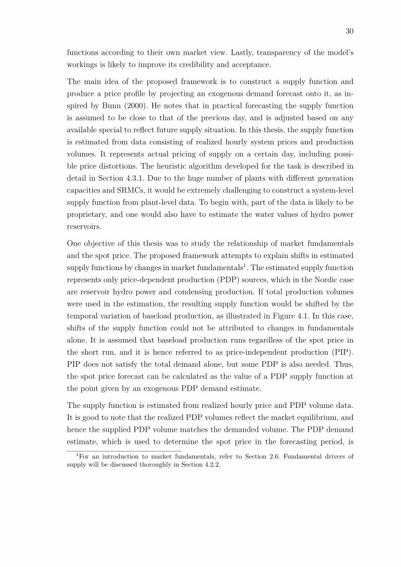
functions according to their own market view. Lastly, transparency of the model’sworkings is likely to improve its credibility and acceptance.

The main idea of the proposed framework is to construct a supply function andproduce a price profile by projecting an exogenous demand forecast onto it, as in-spired by Bunn (2000). He notes that in practical forecasting the supply functionis assumed to be close to that of the previous day, and is adjusted based on anyavailable special to reflect future supply situation. In this thesis, the supply functionis estimated from data consisting of realized hourly system prices and productionvolumes. It represents actual pricing of supply on a certain day, including possi-ble price distortions. The heuristic algorithm developed for the task is described indetail in Section 4.3.1. Due to the huge number of plants with different generationcapacities and SRMCs, it would be extremely challenging to construct a system-levelsupply function from plant-level data. To begin with, part of the data is likely to beproprietary, and one would also have to estimate the water values of hydro powerreservoirs.

One objective of this thesis was to study the relationship of market fundamentalsand the spot price. The proposed framework attempts to explain shifts in estimatedsupply functions by changes in market fundamentals1. The estimated supply functionrepresents only price-dependent production (PDP) sources, which in the Nordic caseare reservoir hydro power and condensing production. If total production volumeswere used in the estimation, the resulting supply function would be shifted by thetemporal variation of baseload production, as illustrated in Figure 4.1. In this case,shifts of the supply function could not be attributed to changes in fundamentalsalone. It is assumed that baseload production runs regardless of the spot price inthe short run, and it is hence referred to as price-independent production (PIP).PIP does not satisfy the total demand alone, but some PDP is also needed. Thus,the spot price forecast can be calculated as the value of a PDP supply function atthe point given by an exogenous PDP demand estimate.

The supply function is estimated from realized hourly price and PDP volume data.It is good to note that the realized PDP volumes reflect the market equilibrium, andhence the supplied PDP volume matches the demanded volume. The PDP demandestimate, which is used to determine the spot price in the forecasting period, is

1For an introduction to market fundamentals, refer to Section 2.6. Fundamental drivers ofsupply will be discussed thoroughly in Section 4.2.2.

31

Total supply volume

Pric

e

Mon 14.02.11 Tue 15.02.11 Wed 16.02.11 Thu 17.02.11 Fri 18.02.11 Sat 19.02.11 Sun 20.02.11

0

10

20

30

40

50

60

70Production volume profile

Time

GW

h/h

PIPPDP

Figure 4.1: Illustration of how the profile of price-independent production (PIP)shifts the location of price-dependent production (PDP) in the supply function oftotal production, even though the pricing of PDP would not change.

derived from the power balance. It is assumed that the equation

Consumption = Production+ Imports− Exports (4.1)

holds for each hour. Here, Consumption and Production are total volumes ofelectricity consumed and produced within the Nordic market, and Imports andExports are total volumes transmitted in/out of the Nordic market area. Further-more, generation sources can be categorized as PIP or PDP. By setting Production =PIP + PDP , we can rewrite (4.1) to define

PDP := Consumption− PIP − Imports+ Exports. (4.2)

Hence, the estimated demand for PDP can be derived from estimates for total con-sumption, PIP, imports and exports. In this thesis, they are considered as exogenousvariables. The actual sources for data will be discussed in Section 4.2.1.

The estimated supply function is assumed to be non-decreasing and piecewise-linear.Nord Pool Spot (2011c) requires that supply curves are non-decreasing, which is areasonable requirement also for the estimated supply function. In this thesis, a singlesupply function is used for each hour of one day. In order that this type of supplyfunction yields expected results, the pricing of PDP must be fairly unambiguous,meaning that same price is asked for same volume of PDP in each hour of the day.Otherwise the supply function cannot correctly represent pricing in each hour.

32

4.1.2 Key assumptions

In what follows, assumptions implied by the proposed framework are summarized.

The system price is determined by matching aggregated supply and demand curvesfor each hour. As described in Section 2.4.1, the Nordic system price is determinedby an implicit auction. The assumption somewhat simplifies the actual pricing mech-anism. In addition to hourly sell and purchase orders, participants can also specifyflexible hour offers and block orders. The hourly orders are matched by intersectingaggregated supply and demand curves for each hour, which yields an equilibriumprice and volume. Flexible hour offers and block orders are activated if they im-prove the social welfare given by the basic allocation. When they are activated,the affected hours have a new equilibrium price. In case of a block order, pricesin the hours covered by the block depend on each other, which is contrary to theassumption.

Physical consumption, production and exchange volumes act as a proxy for Elspotsupply, demand and flow quantities. The system price is determined by the pricesand volumes specified in bids submitted to Elspot, but the proposed frameworkuses physical consumption, production and exchange volumes to approximate thesefinancial quantities. This is necessary, as the framework depends on distinguishingthe contribution of different generation sources in total production. Elspot volumesare closely related to physical volumes, because spot trades involve physical deliveryof power. In 2011, Elspot’s daily turnover amounted on average to 76 % of thephysical turnover. Moreover, correlation between Elspot and physical turnover wasestimated to be 0.99, which strongly supports the validity of the assumption.

Demand is inelastic on short term. Inelasticity of demand is commonly assumed inspot price models, such as in fundamental approaches proposed by Skantze et al.(2000) and Vehviläinen and Pyykkönen (2005), and in autoregressive models de-scribed by Nogales et al. (2002) and Weron and Misiorek (2008). Furthermore, Byeand Hansen (2008) studied elasticities in Norway and Sweden and concluded zeroelasticity in the summer and very low elasticities in the winter.

Generation can be divided to price-dependent (PDP) or price-independent production(PIP). PDP plants have considerable short-run marginal costs (SRMC), and inthe case thermal generation, also start-up costs. A PDP plant runs only when themarket price covers these costs. On the other hand, the SRMC of a PIP plantis remarkably lower than the normal price level, and the production decision is

33

independent of the market price. As described in Section 2.2, the major generationsources in the Nordic countries are hydropower, nuclear power, wind power andconventional thermal generation. Hydropower can be further divided to regulatedand unregulated generation. In conventional thermal generation, a distinction canbe made between CHP and condensing plants. Out of these sources, condensing andregulated hydropower are considered as PDP and the rest as PIP.

The market is perfectly competitive. Under perfect competition, the market priceis equal to the marginal cost of the last unit produced. If the assumption holds,the price should reflect fuel and emissions costs, or water value. As discussed inSection 2.5, the marginal cost of hydro power is the water value. Therefore, theprice should be connected to the market fundamentals which affect the water value.A company exploits market power if it attempts to manipulate prices in order toraise its profits. A number of studies have assessed the presence of market powerin the Nordic market. Kauppi (2009) argues that a part of Nordic hydro powerresources are operated strategically, but under most circumstances the concentrationof market power is not high enough to affect the price level. In their review ofempirical market power studies, Fridolfsson and Tangerås (2009) find no evidenceof systematic exploitation of the Nordic market power on the system level.

4.1.3 Specification of the framework

The proposed framework is essentially summarized by the following steps, whichdescribe how the system price forecast is produced. The steps are outlined in Fig-ure 4.2.

1. Estimation data set is built from hourly realized prices and PDP volumes.

2. PDP supply function is estimated from the data set using a heuristic algorithm(described in Section 4.3.1).

3. For each day for which a forecast is to be made, the supply function estimateis adjusted based on any information on market fundamentals.

4. Demand for PDP is estimated for each day for which a forecast is to be made.The PDP demand estimate is considered as an exogenous variable.

5. System price forecast is calculated as the values of the adjusted supply func-tions at the estimated PDP demand.

34

Inflow forecast

Temperature forecast

Capacity margin

Historical system prices

Historical PDP volumes

Estimated PDP supplyfunction (baseline)

Volume

Price

Forecasted spot price

Time

Price

Supply function

estimationalgorithm

Supply functionadjustment

based on marketfundamentals

Adjusted PDP supplyfunction (Day 1)

Volume

Price

Adjusted PDP supplyfunction (Day 2)

Volume

Price

PDP demand estimate

Time

Volume

Day 1 Day 2

Day 1 Day 2

Market fundamentals (example)

Supply function estimation data

Estimated consumption

Estimated PIP

Net Imports – Exports

Figure 4.2: Outline of the proposed forecasting framework. Exogenous input vari-ables are in grey colour. The data is will be discussed in Section 4.2. The supplyfunction estimation algorithm (red) is described in Section 4.3.1. Changes in the es-timated supply function with respect to market fundaments (blue) will be discussedin Sections 4.3.2 and 4.3.3.

The framework relies on several data sources to determine the volume of PDP. Therealized PDP volume can be directly calculated by summing up price-dependentproduction volumes from appropriate statistics. However, it is significantly harderto create a direct forecast of the PDP demand. Hence, the forecasted PDP demandis derived from the power balance equation as in (4.2). Consumption and PIP areindependent of price, and can therefore be modelled separately or acquired from anexternal source. Exchange between the Nordic market and Central Western Europeis determined in a so-called market coupling process, which sets socially optimalpower flows on the interconnections (European Market Coupling Company, 2009).Connections to Russia have no coupling mechanism, but the exchange depends solelyon the difference between Russian price and Finnish area price. Nevertheless, alsoestimates for exchange can be obtained from external sources.

35

4.2 Description of data

The forecasting approach developed in this chapter is somewhat data-intensive. Ex-haustive production data per generation source are required to determine the volumeof price-dependent production (PDP). Furthermore, market fundamentals are usedto adjust the estimated supply function. The first part of this section describesactual data sources for the Nordic market, and the second part discusses marketfundamentals and their causal effects on the pricing.

4.2.1 Data set

The proposed framework relies on three main categories of data, which are systemprice, production volumes and market fundamentals. Realized system price and PDPvolume are used to construct a supply function estimate, and the price forecast isgiven as the value of the estimated supply function at the forecasted PDP demand.The estimated supply function is adjusted according to relevant changes in themarket fundamentals.

The data can and needs to be obtained both from public and commercial sources.The system price is published by Nord Pool Spot. Actual and historical productiondata per hour and generation source are published by Nordic TSOs, but it mayoccur with a lag that essentially decreases the usability of the data. Fingrid (FI)and Statnett (NO) publish production statistics in real-time, but in the case ofSvenska Kraftnät (SE) and Energinet.dk (DK) the lag ranges from one week toseveral months. Therefore, it is necessary to utilize the services of commercial dataproviders. Commercial data is also needed to forecast the demand of PDP, unless theforecaster has capability to model it themselves. Finally, weather and hydro-relatedfundamentals are typically bought as a service due to highly complex models behindthem.

The framework is based on the volume of PDP instead of total production, as ex-plained in Section 4.1.1. Wind, unregulated hydro power, nuclear power and CHPare considered as PIP, and condensing and regulated hydro power as PDP. The hy-dro power production volumes provided by TSOs do not differentiate unregulatedand regulated hydro production. For that reason, a crude generalization has to bemade so that Finnish and Swedish hydro power is considered as PIP, and Norwe-gian hydro power as PDP. This division is supported by Javanainen (2005), who

36

studied publicly available, aggregated production data, and found that Norwegianhydro production showed stronger price-dependency than Swedish and Finnish hy-dro production. The division between PIP and PDP should definitely be improvedat a later stage. The division used in the empirical part of this thesis is presentedin Table 4.1. Estonia was not included in the data set used in this thesis. It haspractically no effect on the analysis which is conducted on system level, as Estoniamakes up only 2–3 % of total Nordic production.

Table 4.1: Division of generation sources (as reported by the TSOs) into price-independent (PIP) and price-dependent production (PDP). Because regulated andunregulated hydro power were not differentiated, the classification of hydro wasbased on the relatively higher degree of regulation in Norway compared to Swedenand Finland.

Country PIP PDP

Finland Hydro, Nuclear, CHP (industrial),CHP (district heating)

Condensing

Sweden Wind, Hydro, Nuclear, CHP Condensing

Denmark Wind, Local CHPs Central power stations∗

Norway — Hydro∗Includes both district heating CHP and condensing power plants.

4.2.2 Fundamental drivers of supply

An estimated supply function represents pricing in the market at certain point oftime. It is assumed that the pricing depends on the prevailing market fundamentals(Section 2.6). Forecasting requires that the supply function is adjusted in proportionto changes in the fundamentals. This subsection presents main fundamentals anddiscusses their causal effects on electricity pricing. Market data from years 2009–2011is used to illustrate the effects, which are summarized in Table 4.2. The argumen-tation builds strongly on the concept of water value and the dynamics of hydro andthermal generation, which were discussed in Section 2.5.

Volume of price-dependent production (PDP) has a strong effect on the price leveland the periodic variation of the system price. PDP plants have different marginalproduction costs depending on the technology and other plant-specific factors. When

37

the demand for PDP increases, generation capacity with a higher marginal produc-tion cost needs to be activated. There can be big differences between the marginalcosts of peaking power plants, which adds to the price volatility during highestdemand. Under the competitive market assumption, the plant with the highestmarginal cost sets the market price. Furthermore, PDP reflects the periodical vari-ation of consumption, which takes place on intra-day, weekly and yearly levels. Ameasure of consumption or demand is included in the price formula of fundamentalmodels (Section 3.6) or widely used as a predictor variable in time-series models(Section 3.4).

Short-run marginal cost (SRMC) of condensing production has a critical role inthe allocation of hydro and condensing production. As defined in Section 2.2.1, themain factors of SRMC are fuel cost, emission cost and plant efficiency. It should benoted that start-up costs must be also taken into account. The SRMC of an averagecoal condensing plant is considered for price forecasting purposes. Marginal costsare taken into account in long-term models, such as EMPS (Wolfgang et al., 2009),which are used for determining water values. When water values are below SRMC ofcoal condensing, hydro power will precede condensing production in the merit order.Subsequently, the spot price will not exceed the SRMC of condensing production ifthe amount of hydro power offered to the market is enough to satisfy the demandwithout condensing power.

Temperature has a non-linear effect on consumption. When below the level whereheating is needed, power consumed by electrical heating is proportional to the tem-perature. Likewise, but very infrequently in the Nordic countries, electrical coolingdevices begin to increase consumption above a certain temperature level. Especiallyin spring, rising temperatures speed up the melting of snow and ice, which con-tributes to inflow.

Inflow measures the power generation potential of water, and is typically given inenergy units. Fundamental Nordic price models commonly use inflow values aggre-gated per price area or the whole market. According to Laukkanen (2004), inflowmodels take temperature, precipitation, snow reservoirs and soil water as input. Ja-vanainen (2005) studied hydro production in Norway and concluded that inflows arelikely to result in uncontrolled (price-independent) hydro production in areas wherethe production system has low flexibility. As Norway has generally most flexiblehydro production capability in the Nordic market, it can be assumed that hydroproduction in Sweden and Finland depends even more strongly on inflows. As a

38

result, inflows increase PIP, which can be expected to lower the demand for PDP. Inthe face of spillage, inflows can increase the production pressure on price-dependenthydro and thus lower the pricing.

Hydro balance represents the deviation of current water resources from a multi-yearaverage at the same time of the year. The balance calculation includes water in hydroreservoirs, snow and soil. Vehviläinen and Pyykkönen (2005) regard hydro balanceas an indicator of production willingness in their fundamental model. A surplus ofwater resources can limit producers’ flexibility and lower the water values. On theother hand, scant water resources may allow a highly flexible production planning,which can lead to high prices and profits from hydro generation. The Nordic hydrobalance is the sum of regional hydro balances, which can differ depending on thelocal conditions.

As can be seen in Figure 4.3, peaking system prices have occurred during high PDPdemand in the first quarters of 2010 and 2011. During the second and third quartersPDP demand was typically at minimum level, and the system price was somewhatfollowing the level of SRMC Coal. The price profile in these quarters is considerablyflatter than that of PDP. It is likely that price-dependent hydro producers are ableto keep their water values close to, or even above SRMC Coal. Moreover, it can beobserved that most price collapses coincide with sudden increases in inflow. DuringQ3 in 2011 prices collapse below 10 EUR/MWh level, which is possibly due to thecombination of high hydro balance and a rise in inflow. Prices seem to generallyrecover faster from sudden downward movements than upward moments.

Tightness, or the ratio of actual production to available production capacity ofNorwegian hydro production is examined as another indicator of spiking prices.Javanainen (2005) argues that the aggregated supply curve of Norwegian productionis increasing due to hydro power plants having different water values. Differencesbetween plant-specific water values can be substantial towards the high end of thesupply curve. Therefore, high tightness can be a signal for increased price volatility. Itcan be seen in Figure 4.4 that tightness follows the profile of PDP, but has a largerrelative difference between working day and weekend levels. Moreover, extremelyhigh price volatilities appear, when tightness is above 70 %.

To conclude, historical values were used to analyse the relationship of key fun-damentals and system price. The use of historical values is typical for long-termfundamental analyses of the power market, such as Johnsen (2001) and Botterudet al. (2010). However, hydro production planning relies much on the outlook of

39

Table 4.2: Summary of fundamentals affecting the pricing of PDP supply on systemlevel in the Nordic market

Fundamental Effect onpricing

Datafrequency

Main arguments

Hydro balance ↘ week Indicates the level of control that hydroproducers have over regulated(reservoir) production

Inflow ↘ day Increases unregulated hydroproduction, and may increaseproduction pressure of regulated hydro

Precipitation ↘ day Input of inflow calculation

Temperature ↘ day Inverse relation to consumption mayaffect water valuation. Input of inflowcalculation

SRMC Coal ↗ day Direct effect on the pricing ofcondensing production. Reflects theopportunity cost of withdrawn hydroproduction

Tightness ↗ hour The higher the utilization, the moreexpensive plants are brought on-line

weather fundamentals. Uncertainty in weather forecasts may lead to ex-post subop-timal water values and production allocation. Example 1: A producer allocates waterto be used in the following weeks when low precipitation is forecasted. If the fore-cast later turns wet, the producer may earn less profit due to increased run-of-riverproduction. Example 2: A producer allocates water for week 1 in January, becausetemperatures are expected rise in week 2. Later the temperature forecast for week 2turns considerably colder, which increases the consumption forecast. Consequently,water values for week 1 were set too low.

40

Q1−09 Q2−09 Q3−09 Q4−09 Q1−10 Q2−10 Q3−10 Q4−10 Q1−11 Q2−11 Q3−11 Q4−11

0

20

40

60

80

100

120System price & SRMC Coal

EU

R/M

Wh

System priceSRMC Coal

Q1−09 Q2−09 Q3−09 Q4−09 Q1−10 Q2−10 Q3−10 Q4−10 Q1−11 Q2−11 Q3−11 Q4−11

0

1000

2000Inflow & hydro balance

GW

h/da

y (I

nflo

w)

Q1−09 Q2−09 Q3−09 Q4−09 Q1−10 Q2−10 Q3−10 Q4−10 Q1−11 Q2−11 Q3−11 Q4−11

−5

0

5x 10

4G

Wh

(Hyd

ro b

alan

ce)

Inflow (Norway)Hydro balance (Norway + Sweden)

Q1−09 Q2−09 Q3−09 Q4−09 Q1−10 Q2−10 Q3−10 Q4−10 Q1−11 Q2−11 Q3−11 Q4−11

1

2

3

4

5

6

7

8x 10

5 PDP

GW

h

PDP (daily)PDP (weekly mean)

Figure 4.3: Historical values of the median system price, SRMC Coal, inflow, hydrobalance and PDP

41

Q1−10 Q2−10 Q3−10 Q4−10 Q1−11 Q2−11 Q3−11 Q4−11

0

20

40

60

80

100

120

140

160

EU

R/M

Wh

Median system price & tightness

Q1−10 Q2−10 Q3−10 Q4−10 Q1−11 Q2−11 Q3−11 Q4−11

20

30

40

50

60

70

80

90

100

Tig

htne

ss (

%)

Median system priceMedian tightness

Q1−10 Q2−10 Q3−10 Q4−10 Q1−11 Q2−11 Q3−11 Q4−11

25

25.5

26

26.5

27

27.5

28

28.5

29

29.5

30

GW

(C

apac

ity)

Available hydro capacity & PDP

Q1−10 Q2−10 Q3−10 Q4−10 Q1−11 Q2−11 Q3−11 Q4−11

0

100

200

300

400

500

600

700

800

900

1000

GW

h/da

y (P

DP

)

Available hydro capacityPDP (daily)

Figure 4.4: System price and utilization of Norwegian hydro power capacity (Tight-ness)

42

4.3 Validation of the framework

This section describes how the proposed forecasting framework was validated againsthistorical market data with a backtesting procedure. The data set used for valida-tion is described in Section 4.2 and spans over the years 2009–2011. Because PDPvolume is an external variable in the framework, the validation focuses on the es-timation of the supply function and the effects of changes in market fundamentals.The validation procedure used realized PDP volume both for estimating the supplyfunction and for calculating the forecast price. In effect, the forecast error, definedas the difference of realized and forecasted price, was completely attributed to theinaccuracy of the supply function.

4.3.1 Estimating the supply function

The PDP supply function represents the pricing of electricity in the Nordic marketon a certain day. As part of this thesis, a heuristic algorithm was developed toestimate a supply function from data consisting of observed hourly system pricesand corresponding PDP volumes. The algorithm approximates the data with a firstdegree spline. It is basically a piecewise defined function that connects the datapoints chosen as knots with line segments. Furthermore, it is assumed that thesupply function is non-decreasing.

Constructing a supply function is unambiguous if each PDP volume in the data setis associated with a certain price at all times. In this case, the plotted data pointsalign to a single curve as illustrated by the upper curve in Figure 4.5. On the otherhand, it is possible that a certain volume has been traded at different prices duringthe same day, as illustrated by the lower curve in Figure 4.5. In that case the supplyfunction cannot represent correct pricing for each hour of the day. The estimationalgorithm deals with the unambiguity by prioritizing more recent observations overless recent ones.

The estimation algorithm has three major phases. In Phase I, the data is split intofixed-size volume intervals, and the most recent observation from each interval isstored. In Phase II, stored observations belonging to the most recent calendar dayare selected as knots. In Phase III, older stored observations are selected as knots aslong as their inclusion does not violate the requirement for a non-decreasing functionshape.

43

1.4 1.6 1.8 2 2.2 2.4 2.6

x 104

58

60

62

64

66

68

70

72Estimated supply functions

PDP (MWh/h)

Pric

e (E

UR

/MW

h)

Hourly prices for Thu 03.03.2011Estimated supply function for Thu 03.03.2011Hourly prices for Thu 10.03.2011Estimated supply function for Thu 10.03.2011

Figure 4.5: Illustration of unambiguous and ambiguous pricing. On 3.3.2011 samevolumes have been traded at fairly similar prices in all hours. In contrast, on10.3.2011 there is a 1.20 EUR/MWh difference in the volume range of 18 GWh/hbetween different hours.

Let xi = {ti, qi, pi} denote an observation at time (hourly resolution) ti, PDP volumeqi and system price pi. If ti < tj, then time ti precedes tj. Given an estimation dataset X = {xi} and volume interval size vint, the algorithm is defined as follows:

phase ISet XMostRecent = ∅Set lower volume bound l = min {qi}repeat

Set upper volume bound u = l + vint

Add xk to XMostRecent s.t. tk = max {ti | l ≤ qi ≤ u}Set l = u

until l > max {qi}phase IIDefine D := “set of calendar days for which there are observations in XMostRecent”

44

Set dmax = maxDDefine Xd

MostRecent := “observations in XMostRecent belonging to calendar day d ∈D”Set XSupplyF unction = Xdmax

MostRecent

phase IIIfor each d ∈ D\ {dmax} do

Iterate d from the most recent to the least recent dayfor each xi ∈ Xd

MostRecent doIterate xi from the smallest to the largest volume qi

if qi < qj & pi < pj ∀ xj ∈ XSupplyF unction

or qi > qj & pi > pj ∀ xj ∈ XSupplyF unction

or ∃ xj ∈ XSupplyF unction

s.t. qj < qi & pj < pi & qi < qj+1 & pi < pj+1then

Add xi to XSupplyF unction

end ifend for

end forReturn XSupplyF unction

It should be emphasized that the estimation algorithm was developed primarily forthe purpose of evaluating and validating the proposed framework against historicalmarket data. It enabled automatic and non-interactive estimation of supply func-tions, which was necessary as several years of historical data was processed. In a liveforecasting situation more time can typically be invested into the estimation process,and the quality of the estimate could be improved by checking the unambiguity ofpricing and by making manual adjustments to the estimated function.

4.3.2 Forecasting with a static supply function

As the first stage of validation, prices were predicted using a single PDP supplyfunction for the whole forecasting period. A situation was considered, where thesupply function is estimated from most recent realized price and PDP volume datausing the algorithm presented in the previous subsection. The so-obtained supplyfunction was used to statically represent pricing of PDP throughout the forecastingperiod. The forecast price was determined as the value of the supply function at thedemand of the moment.

45

A forecast is typically done before Elspot’s gate closure at 12:30 CET, so that theresults can be used to adjust the bids. Spot prices for the current day are knownat that time, and theoretically it is possible to observe realized PDP volumes up tothe last full hour. In reality, the availability of PDP data varies depending on thedata providers, as noted in Section 4.2.1. If it is desired to use only realized datafor supply function estimation, a lead time of one day should be assumed betweenthe estimation and forecasting periods. The lead time can be reduced by extendingthe estimation data set with actual prices and PDP volumes estimated for the non-realized hours of the current day.

In what follows, observations from the validation experiments will be discussed. Thelevel of PDP in validation data was highly volatile, and it was common that PDPdemand in the forecasting period could go out of the range where the PDP supplyfunction was defined. This was usually connected to changes in total consumption.One reason were differences in consumption levels during working days and theweekend, and another reason were changes in outside temperature, which affectedthe load from electrical heating. Possible solutions for the issue are extrapolatingthe supply function, or extending the estimation period so that it would cover thedesired volume range. Both solutions have their limitations.

Extrapolation of the supply function, especially to higher volumes, depends essen-tially on the maximum available capacity of PDP. It is likely that best extrapolationcan be achieved by manually extending the supply curve, while taking fundamen-tals into account. Given that the additional supply data is consistent with the morerecent data, extending the estimation period extends the volume bounds, where thesupply function is defined. As pointed out in Section 4.3.1, the estimation algorithmfirst uses most recent data, and then adds data points which are consistent with theincreasing slope of the function. In this validation procedure, the estimation periodwas extended to match the volume range in forecasting period. If PDP values werestill out of bounds, no price was forecasted for the concerned hour.

The accuracy of forecasts with a static supply function degraded rapidly as thelead time increased. The effect was studied by forecasting the price one day aheadwith lead times of 0, 1 and 3 days. The length of the estimation period was 21days, but the estimation algorithm typically exploited only 2–5 most recent days.A number of time periods were selected from the data set to represent differentseasons. As illustrated by Figure 4.6, short lead times generally produced moreaccurate forecasts. Because the validation was carried out by using realized PDP

46

values both for supply function estimation and forecasting, there is no uncertaintyin the demand side. Therefore, all forecast errors were viewed as an indication thatthe static supply function did not represent true pricing at the time of the forecast.If the pricing was unambiguous, the forecast error could be reduced by adjusting thesupply function. On the other hand, the forecast error can also be due to ambiguouspricing, which cannot be represented by the supply function.

Wed 01.09. Thu 02.09. Fri 03.09. Sat 04.09. Sun 05.09. Mon 06.09. Tue 07.09. Wed 08.09. Thu 09.09. Fri 10.09.

40

42

44

46

48

50

52

54Actual and forecasted price

Pric

e (E

UR

/MW

h)

ActualForecast (Lead 0)Forecast (Lead 1)Forecast (Lead 3)

Wed 01.09. Thu 02.09. Fri 03.09. Sat 04.09. Sun 05.09. Mon 06.09. Tue 07.09. Wed 08.09. Thu 09.09. Fri 10.09.

0.8

1

1.2

1.4

1.6

1.8

2x 10

4 Demand for price−dependent production (PDP)

PD

P (

MW

h/h)

Figure 4.6: The upper plot shows the realized price and forecasts with different leadtimes. The lower plot shows the corresponding demand for PDP. The data is fromSeptember 2010.

The unambiguity of pricing was checked as part of validation. Even if the piecewise-linear supply function is incapable of representing the actual pricing, price trajecto-ries of realized hourly prices and PDP volumes can be used to study shifts in thepricing of supply. Figure 4.7 illustrates the approach with the same time period as inFigure 4.6. It can be seen that pricing was relatively unambiguous from 30.8. to 1.9.except for the highest volumes. The clearest example is 30.8., when the trajectoryformed a small ‘loop’ in the high end of the volume range: The volume was about17 GWh during two hours, but in one hour the price was around 49 EUR/MWh,whereas it was about 1.5 EUR/MWh more during the other hour. It can be also

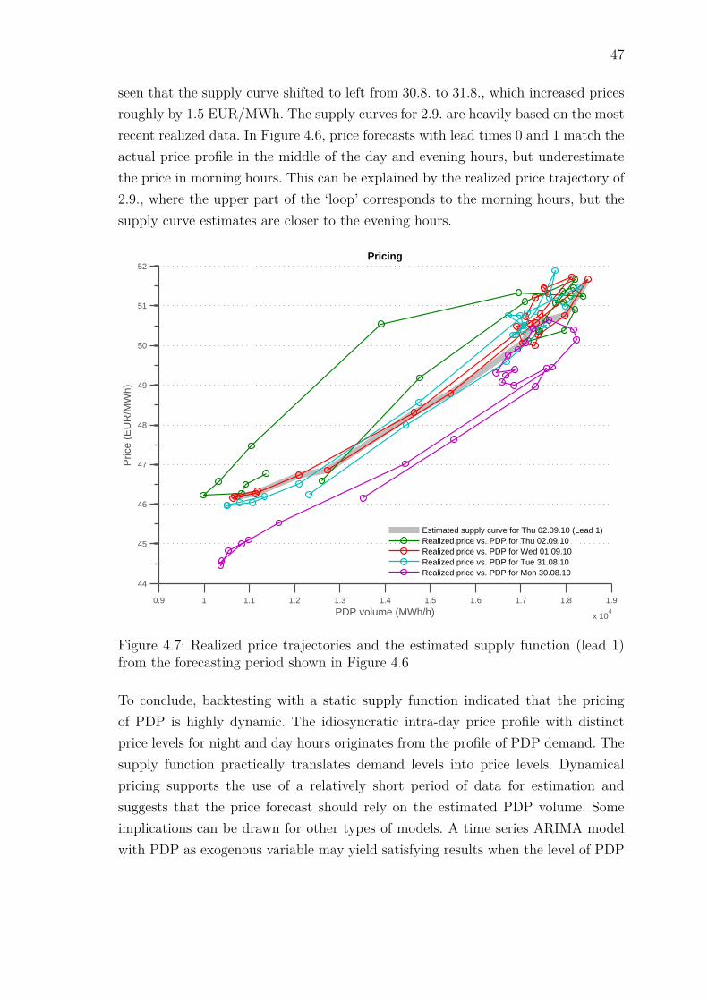
47

seen that the supply curve shifted to left from 30.8. to 31.8., which increased pricesroughly by 1.5 EUR/MWh. The supply curves for 2.9. are heavily based on the mostrecent realized data. In Figure 4.6, price forecasts with lead times 0 and 1 match theactual price profile in the middle of the day and evening hours, but underestimatethe price in morning hours. This can be explained by the realized price trajectory of2.9., where the upper part of the ‘loop’ corresponds to the morning hours, but thesupply curve estimates are closer to the evening hours.

0.9 1 1.1 1.2 1.3 1.4 1.5 1.6 1.7 1.8 1.9

x 104

44

45

46

47

48

49

50

51

52

PDP volume (MWh/h)

Pric

e (E

UR

/MW

h)

Pricing

Estimated supply curve for Thu 02.09.10 (Lead 1)Realized price vs. PDP for Thu 02.09.10Realized price vs. PDP for Wed 01.09.10Realized price vs. PDP for Tue 31.08.10Realized price vs. PDP for Mon 30.08.10

Figure 4.7: Realized price trajectories and the estimated supply function (lead 1)from the forecasting period shown in Figure 4.6

To conclude, backtesting with a static supply function indicated that the pricingof PDP is highly dynamic. The idiosyncratic intra-day price profile with distinctprice levels for night and day hours originates from the profile of PDP demand. Thesupply function practically translates demand levels into price levels. Dynamicalpricing supports the use of a relatively short period of data for estimation andsuggests that the price forecast should rely on the estimated PDP volume. Someimplications can be drawn for other types of models. A time series ARIMA modelwith PDP as exogenous variable may yield satisfying results when the level of PDP

48

volume remains stable. However, the model is linear with respect to PDP and maynot capture steeply increasing prices, which occur when PDP approaches the limit ofavailable production capacity. This problem could be alleviated by applying a moresophisticated ARIMA-GARCH model, which could measure the dynamic volatility(Section 3.4). An artificial neural network model could possibly benefit from a longestimation data set, which can be used to train the model (Section 3.5). It may alsobe able handle the intra-day dynamics better than a static supply function. However,the proposed framework provides higher transparency over price formation. Finally,it should be emphasized that the framework depends heavily on the quality of theestimated supply function.

4.3.3 Analysing the effects of changing fundamentals

As the second stage of validation, the forecast error of the static PDP supply functionwas studied with regression analysis. Analysis of supply functions showed that thepricing of PDP varies in relation to time. Under the assumption of competitivepricing, the variations can be connected to fundamental price drivers discussed inSection 4.2.2. The regression models studied in this subsection attempt to explain therealized price by correcting the output of the static supply function with fundamentalpredictors. The estimation algorithm produces supply functions, which resemblepricing at the end of the estimation period. Parameters were estimated by fittingthe regression model to the whole estimation period using ordinary least squares.

The proposed framework operates on hourly frequency, and the fundamental predic-tors should likewise have a high frequency to distinguish hours. fundamentals withweekly frequency, such as actual hydro balance, are effectively constant within theforecasting horizon. Out of the fundamentals discussed in Section 4.2.2, the follow-ing were included in the regression analysis: inflow in Norway, consumption-weightedaverage temperature in Norway and Sweden, supply tightness in Norway, and thesystem-level PDP. Inflow and temperature had daily frequency, while tightness andPDP were specified on hourly level.

Experiments were made with three different regression models. Linear models werechosen because they can approximate non-linear effects, and parameter estimationis simple. A fundamental predictor for day d and hour h was defined as

xd,h = fd,h − f , (4.3)

49

where fd,h is the actual value of the fundamental, and f is a base value from theestimation period. f Inflow and fT emperature were defined as the average of days, fromwhich data points were included in the supply function estimate (typically 2–3 days).In order not to lose a level of detail, the base value for tightness was defined asfT ightness = fT ightness

h , the average value of hour h over days, from which data pointswere included in the supply function estimate.

In the first experiment, pure differences were used as predictors, resulting in themodel

pd,h = β0 + β1p0d,h + β2x

Inflowd,h + β3x

T emperatured,h + β3x

T ightnessd,h + εd,h, (4.4)

where p0d,h is the price forecast given by the supply function estimate at PDP de-

mand qd,h, βi are the regression coefficients and εd,h is the error term. The secondexperiment used interactions of PDP and the fundamental predictors as variables,specified as

pd,h = β0 + β1p0d,h + qd,h

(β2x

Inflowd,h + β3x

T emperatured,h + β4x

T ightnessd,h

)+ εd,h. (4.5)

The third experiment extended the interaction model by adding future values offundamental predictors. Future values of 1–5 days ahead were used with weightsidentical to the actual value. With predictors up to 5 days ahead, the model was

pd,h = β0 + β1p0d,h + qd,h

(β2x

Inflowd+0,h + · · ·+ β7x

Inflowd+5,h

+ β8xT emperatured+0,h + · · ·+ β13x

T emperatured+5,h (4.6)

+ β14xT ightnessd+0,h + · · ·+ β19x

T ightnessd+5,h

)+ εd,h.

The regression models were backtested against the validation data set. Time peri-ods were selected to represent different seasons and fundamental situations, such asperiods when fundamentals are very stable or change rapidly. Length of the esti-mation period was 14 days, and the forecast was made 7 days ahead with no leadbetween estimation and forecasting periods. For temperature and tightness, realizedvalues were used both in the estimation and forecasting periods. For inflow realizedvalues were available only on weekly level. Hence, values from a time series of latestforecasts for each day were used instead.

Conclusions were made by analysing the error terms and the estimated regressioncoefficients. It was checked if the predictors were statistically significant and if their

50

signs corresponded to the expected fundamental effects, which are summarized inTable 4.2. Overall, the interaction model (4.5) performed better than the basic model(4.4). This could be expected, as correlation between the realized price and PDPdemand was noticed in the analysis of supply curve behaviour (Section 4.2.2). Thethird model (4.6) produced a high goodness of fit due to the high number of variablesin the model, but it did not produce better forecasts then the interaction model.

The regression analysis did not produce reliable quantitative results, which could beused to adjust the price forecasted by an estimated supply function. However, thefollowing conclusions could be made based on the analysis. The regression coefficientscould not be regarded as constant during the estimation and forecasting periods,which together spanned 21 days. Best results were produced under conditions, wherethe values of the fundamental predictors in the forecasting period remained withinthe same limits as in the estimation period. If the values changed significantly, themodel typically under or overestimated the effect. This was particularly noticedwith inflow and temperature. In the studied models, the effect of a fundament wasdirectly proportional to its value difference. However, the findings suggest that theeffects are non-linear even on the very short term. In several cases the price givenby the regression model was inferior to the output of the static supply function,because fundamental predictors adjusted the price in the wrong direction.

4.4 Facilitating price forecasts in practice

This section sums up experiments conducted with the proposed forecasting frame-work and puts forward how the framework can benefit day-to-day forecasting activ-ities.

Realized volumes of price-dependent production (PDP) are needed for supply func-tion estimation. They can be calculated from the power balance as in (4.2), or bydirectly summing up PDP volumes from appropriate statistics. Hourly productionstatistics per generation source are required in both cases, and in principle the datais publicly available. Nord Pool Spot publishes total consumption, production andexchange volumes, and each TSO reports hourly production statistics per generationsource. However, the Swedish and Danish TSOs publish production statistics with aconsiderable lag, which can be several months in the former case and about 10 daysin the latter. In effect, the public data is of little value, and the forecaster must turn

51

to commercial data providers, which are capable of supplying up-to-date figures.

The estimate of future PDP demand is an external variable in the framework. Sim-ilarly to the realized values, the estimate can be derived from the power balance byusing forecasted values, or an external PDP forecast may be used. The forecastershould take into account that the estimate for PDP implies certain expectations onconsumption, exchange and PIP. Moreover, the exchange implies a certain price dif-ference between markets. Major adjustments in the supply function may affect theprice difference to such extent that the direction of the exchange reverts, which couldin turn change the whole PDP estimate. Furthermore, the estimate should reflectreductions in consumption, production or available transmission capacity events asindicated by Nord Pool Spot’s urgent market messages (UMMs).

A PDP supply function that represents the actual pricing of a particular day is thebasis for building estimates for following days. The estimation algorithm presented inSection 4.3.1 can be used to produce a crude estimate, which should be reviewed andtuned by the forecaster. In particular, it should be checked whether the pricing hasbeen unambiguous. If not, special consideration is needed, because a single supplyfunction cannot represent the price in each hour of the day. Moreover, the forecastermust extrapolate the supply function estimate to cover the volume range of PDPdemand in the forecasting period, if the future demand differs from the volumesobserved in the estimation period.

Statistical modelling of short-term fundamental effects turned out to be extremelychallenging. Supply curves can be used to measure changes in pricing, but it is upto the forecaster to connect the changes with market fundamentals. Likewise, theforecaster should take a view on the fundamentals and adjust the supply functionestimates for each day in the forecasting period.

Chapter 5

Conclusions

The purpose of this thesis was to develop and evaluate a framework for forecastinghourly spot prices of electricity in the Nordic market up to one week ahead. Thistype of short-term price forecasts can be used to support operational planning andelectricity trading decisions. Only a few references related to fundamental short-term price forecasts in the Nordic market were found (Dueholm and Ravn, 2004;Javanainen, 2005). Overviews of electricity price forecasting can be found e.g. inBunn (2000), Bunn and Karakatsani (2003) and Weron and Misiorek (2006).

The research method of this thesis consisted of two parts. First, Nordic marketdata was studied in order to identify fundamental drivers affecting price formation,and second, a forecasting framework was designed. The empirical part of the thesisconsisted of implementing the framework and validating it against actual marketdata from years 2009–2011. As a major part of the implementation, an algorithmwas created to estimate aggregated supply functions from market data. Finally, aneffort was made to explain changes in estimated supply functions by changes inmarket fundamentals.

The framework proposed in this thesis was based on a fundamental approach inspiredby Bunn (2000), who argues that a short-term price profile can be forecasted byconstructing a supply function and projecting a demand estimate onto it. In this thisthesis the approach was developed further to match the idiosyncrasies of the Nordicmarket. The supply function was estimated from realized prices and productionvolumes. Thus, it represented actual pricing on a certain day, including possibleprice distortions due to market inefficiency or other reasons. The production andconsumption volumes considered only price-dependent production (PDP). If total

52

53

volume of production would be used, the estimated supply functions would be shiftedby temporal variation in the volume of price-independent production (PIP). Whenonly PDP volumes were used, shifts in the supply functions could be attributed tochanges in water values, short-run marginal costs and related market fundamentals.

The empirical results showed that the spot price was highly volatile and that theeffects of market fundamentals have complex dynamics. These effects arise fromthe supply side, whereas the short-term demand is quite predictable. The pricetrajectories of realized PDP volumes changed from day to day, and occasionally thepricing differed between the hours of a single day. The supply function estimationalgorithm exploited typically data from the previous 2–5 days, while older prices wereincompatible with the requirement for a non-decreasing supply function estimate.The results support the chosen approach, which relies on a small estimation dataset and emphasizes importance of forecasts for market fundamentals. It is unlikelythat statistical models with constant parameters would yield satisfying results.

Experiments with historical market data indicated that the framework was able toreproduce reasonable hourly price profiles, when the realized PDP volume was usedas the demand. The results were highly sensitive to the estimated supply functions.Another challenge arose from cases, where the level of PDP demand in the estimationperiod was significantly different compared to the forecasting period. As a result,the estimated supply function was not defined for extreme values of PDP demand inthe forecasting period. Automatic and/or statistical extrapolation of the estimatedsupply function turned out to be difficult, because its shape depends on fundamentalfactors. This could be necessary, for instance, if the temperature changes drastically.

Based on the results, it can be suggested that model user’s input is incorporatedwith the estimation of supply functions. It may have several advantages when theframework is used in day-to-day forecasting. An experienced user is likely to surpassthe estimation algorithm in accuracy. Instead of relying only on statistical data, theuser can use their own view and interpret any information that could potentially havean effect on the pricing. The regression models used to explain changes in supplyfunctions with fundamental changes did not produce reliable quantitative results.However, the trajectories of realized prices and PDP volumes can be used to studyday-on-day changes in the pricing of supply. Combined with access to fundamentaldata, the analysis of trajectories can be useful in building market insight.

The scope of this thesis was limited to the Nordic system price, which is calcu-lated without considering the limitations of transmission capacity between bidding

54

areas. When a transmission line becomes congested, the concerned bidding areaswill have different area prices. Other limitations arise from the assumptions madein the framework. It should be noted that the framework assumes that the supplyfunction of PDP is constant within a day. The empirical studies revealed that theassumption does not hold all the times. Therefore, it is advised that the model userexamines the data used for estimation in order to assess the validity of the assump-tion. Moreover, it is probable that the accuracy of empirical results suffered fromthe high-level aggregation of production volume data. Based on the available data,production volumes had to be classified as PIP or PDP by generation technologyand country. The data did not differentiate regulated and unregulated hydro powergeneration. As a result, all Swedish and Finnish hydro power was considered to bePIP, even though it has some room for price-based regulation. Norwegian hydropower was considered to be fully PDP.

Further studies could concentrate on extending the proposed forecasting framework.A logical follow-up would be to model the area prices. As a starting point, the currentframework could be applied to a single price area by modelling the area-specific PDPsupply function, demand and exchange. Another improvement could be to treat theexchange in/out of the Nordic market (or between bidding areas) as an endogenousvariable. At present exchange is assumed to be exogenous, while its direction andvolume actually depend on the differences of area prices in the concerned areas.Furthermore, the supply function estimation technique has room for improvement.The heuristic algorithm presented in this thesis uses only historical price and volumedata. It could be possible to attain more accurate supply functions by adjustingthe estimate based on production tightness or other market fundamentals. Moreattention should be also given to modelling changes in the supply function as afunction of market fundamentals. In this thesis, the analysis of fundamentals wasbased on realized historical values. If appropriate data could be obtained, it wouldbe interesting to study if supply curve changes could be explained better by changesin consecutive fundamental forecasts. It seems possible, because water values andhydro power production schedules are based on future expectations.

Bibliography

Andersson B., Bergman L. (1995). Market structure and the price of electricity: Anex ante analysis of the deregulated Swedish electricity market. The Energy Journal16(2) pp. 97–109.

Angelus A. (2001). Electricity price forecasting in deregulated markets. The Electric-ity Journal 14(3) pp. 32–41.

Baldick R., Grant R., Kahn E. (2004). Theory and application of linear supply func-tion equilibrium in electricity markets. Journal of Regulatory Economics 25(2)pp. 143–167.

Borenstein S., Bushnell J., Knittel C.R. (1999). Market power in electricity markets:Beyond concentration measures. The Energy Journal 20(4) pp. 65–88.

Botterud A., Kristiansen T., Ilic M.D. (2010). The relationship between spot andfutures prices in the Nord Pool electricity market. Energy Economics 32(5) pp.967–978.

Box G.E.P., Jenkins G.M. (1976). Time Series Analysis: Forecasting and Control.Holden-Day, Oakland, California.

Bunn D.W. (2000). Forecasting loads and prices in competitive power markets. Pro-ceedings of the IEEE 88(2) pp. 163–169.

Bunn D.W., Karakatsani N.V. (2003). Forecasting electricity prices. Working pa-per, London Business School. Also available as http://www.erasmusenergy.com/downloadattachment.php?aId=f1b845f3419ea055a3fe6fe11ac95ca8&articleId=50.

Bunn D.W., Oliveira F. (2001). Agent-based simulation-an application to the newelectricity trading arrangements of England and Wales. IEEE Transactions onEvolutionary Computation 5(5) pp. 493–503.

Bye T., Bruvoll A., Aune F.R. (2006). The importance of volatility in inflow ina deregulated hydro-dominated power market. Discussion papers no. 472, Statis-tics Norway, Research Department. Also available as http://www.ssb.no/cgi-bin/publsoek?job=forside&id=dp-472&kode=dp&lang=en.

Bye T., Hansen P.V. (2008). How do spot prices affect aggregate electricity demand?Discussion papers no. 527, Statistics Norway, Research Department.

55

56

Catalão J., Mariano S., Mendes V., Ferreira L. (2007). Short-term electricity pricesforecasting in a competitive market: A neural network approach. Electric PowerSystems Research 77(10) pp. 1297–1304.

Dueholm L., Ravn H.F. (2004). Modelling of short term electricity prices, hydroinflow and water values in the Norwegian hydro system. In 6th IAEE EuropeanConference. Also available as http://www.balmorel.dk/Doc/ShortTermHydro2004.pdf.

European Market Coupling Company (2009). EMCC Optimizer 2.0. Technical re-port. Also available as http://www.marketcoupling.com/document/1137/EMCC%20Optimizer.pdf.

Eurostat (2012). Supply, transformation, consumption – electricity – annual data[nrg_105a]. Statistical database. Available as http://appsso.eurostat.ec.europa.eu/nui/show.do?dataset=nrg_105a.

Eydeland A., Wolyniec K. (2003). Energy and Power Risk Management. Wiley.

Flatabø N., Doorman G., Grande O., Randen H., Wangensteen I. (2003). Experi-ence with the Nord Pool design and implementation. IEEE Transactions on PowerSystems 18(2) pp. 541–547.

Fosso O., Gjelsvik A., Haugstad A., Mo B., Wangensteen I. (1999). Generationscheduling in a deregulated system. The Norwegian case. IEEE Transactions onPower Systems 14(1) pp. 75–81.

Fridolfsson S.O., Tangerås T.P. (2009).Market power in the Nordic electricity whole-sale market: A survey of the empirical evidence. Energy Policy 37(9) pp. 3681–3692.

Førsund F.R. (2007). Hydropower Economics. Springer.

Gao F., Xiaohong G., Cao X.R., Papalexopoulos A. (2000). Forecasting power mar-ket clearing price and quantity using a neural network method. In 2000 PowerEngineering Society Summer Meeting, pp. 2183–2188, IEEE.

Garcia R., Contreras J., van Akkeren M., Garcia J. (2005). A GARCH forecastingmodel to predict day-ahead electricity prices. IEEE Transactions on Power Systems20(2) pp. 867–874.

Geman H., Roncoroni A. (2006). Understanding the fine structure of electricityprices. The Journal of Business 79(3) pp. 1225–1261.

Gibbons R. (1992). A Primer in Game Theory. Prentice Hall.

Green R.J., Newbery D.M. (1992). Competition in the British electricity spot market.Journal of Political Economy 100(5) pp. 929–953.

Guthrie G., Videbeck S. (2007). Electricity spot price dynamics: Beyond financialmodels. Energy Policy 35(11) pp. 5614–5621.

57

Haykin S. (1994). Neural Networks: A Comprehensive Foundation. Prentice HallInternational.

Huisman R., Huurman C., Mahieu R. (2007). Hourly electricity prices in day-aheadmarkets. Energy Economics 29(2) pp. 240–248.

Jabłonska M. (2011). From fluid dynamics to human psychology. What drives fi-nancial markets towards extreme events. Ph.D. thesis, Lappeenranta Universityof Technology.

Javanainen T. (2005). Analysis of short-term hydro power production in the Nordicelectricity market. Master’s thesis, Helsinki University of Technology.

Jónsson T. (2008). Forecasting of electricity prices: Accounting for wind power pre-dictions. Master’s thesis, Technical University of Denmark.

Johnsen T.A. (2001). Demand, generation and price in the Norwegian market forelectric power. Energy Economics 23(3) pp. 227–251.

Kalatie S. (2005). Sähkön markkinahintaa selittävät tekijät. Master’s thesis,Lappeenranta University of Technology.

Kanamura T., Ohashi K. (2007). A structural model for electricity prices with spikes:Measurement of spike risk and optimal policies for hydropower plant operation.Energy Economics 29(5) pp. 1010–1032.

Kara M. (editor) (2004). Energia Suomessa: Tekniikka, talous ja ympäristövaikutuk-set. VTT Prosessit, Edita Prima Oy.

Karakatsani N.V., Bunn D.W. (2008a). Forecasting electricity prices: The impact offundamentals and time-varying coefficients. International Journal of Forecasting24(4) pp. 764–785.

Karakatsani N.V., Bunn D.W. (2008b). Intra-day and regime-switching dynamics inelectricity price formation. Energy Economics 30(4) pp. 1776–1797.

Kauppi O. (2009). A model of imperfect dynamic competition. Ph.D. thesis, HelsinkiSchool of Economics.

Kumar David A., Wen F. (2001). Market power in electricity supply. IEEE Trans-actions on Energy Conversion 16(4) pp. 352–360.

Laukkanen A. (2004). Short term inflow forecasting in the Nordic power market.Master’s thesis, Helsinki University of Technology.

Livanis E., Zapranis A. (2007). Forecasting the day-ahead electricity price in NordPool with neural networks: Some preliminary results. Technical report, EnergyInformation Administration, Office of Integrated Analysis and Forecasting, U.S.Department of Energy. Also available as http://papers.ssrn.com/sol3/papers.cfm?abstract_id=1568939.

58

Meyer-Brandis T., Tankov P. (2008). Multi-factor jump-diffusion models of electric-ity prices. International Journal of Theoretical and Applied Finance 11(05) pp.503–528.

Nogales F., Contreras J., Conejo A., Espinola R. (2002). Forecasting next-day elec-tricity prices by time series models. IEEE Transactions on Power Systems 17(2)pp. 342–348.

Nord Pool Spot (2011a). Company presentation. Accessed on 15.3.2011.http://nordpoolspot.com/Global/Download%20Center/Annual-report/Nord-Pool-Spot-Company-Presentation_2011.pdf

Nord Pool Spot (2011b). The Nordic electricity exchange and the Nordic model fora liberalized electricity market. Accessed on 4.10.2011.http://nordpoolspot.com/Global/Download%20Center/Rules-and-regulations/The-Nordic-Electricity-Exchange-and-the-Nordic-model-for-a-liberalized-electricity-market.pdf

Nord Pool Spot (2011c). Trading appendix 2a: Elspot market regulations. Accessedon 4.6.2012.http://nordpoolspot.com/Global/Download%20Center/Rules-and-regulations/trading-appendix_2-a_elspot-market-regulations_01jan2011.pdf

NordREG (2012). Nordic market report 2012: Development in the Nordic electric-ity market. Technical report. Also available as https://www.nordicenergyregulators.org/Publications/.

Pindyck R.S. (1999). The long-run evolution of energy prices. The Energy Journal20(2) pp. 1–27.

Queiroz A., Oliveira F., Lima J.M., Balestrassi P. (2007). Simulating electricity spotprices in Brazil using neural network and design of experiments. In 2007 IEEELausanne Power Tech, pp. 2029–2034.

Ravn H.F. (2001). Balmorel: A model for analyses of the electricity and CHP mar-kets in the Baltic sea region. Technical report, Balmorel Project. Also available ashttp://www.eabalmorel.dk/index.php?option=com_content&view=article&id=32:balmorel-a-model-for-analyses-of-the-electricity-and-chp-markets-&catid=2:pub&Itemid=22.

Seebregts A.J., Goldstein G.A., Smekens K. (2001). Energy/Environmental mod-eling with the MARKAL family of models. In OR2001 Conference, Energy andEnvironment Session.

Skantze P., Gubina A., Ilic M.D. (2000). Bid-based stochastic model for electricityprices: The impact of fundamental drivers on market dynamics. Energy Labora-tory Publications MIT EL 00–004, Massachusetts Institute of Technology.

Szkuta B., Sanabria L., Dillon T. (1999). Electricity price short-term forecasting

59

using artificial neural networks. IEEE Transactions on Power Systems 14(3) pp.851–857.

Vehviläinen I., Bröckl M., Virtanen E., Kallio M. (2010). Nordic electricitypeak prices during the winter 2009-2010. Technical report, Gaia ConsultingOy. Also available as http://www.energiamarkkinavirasto.fi/files/Gaia_Raportti_20100930.pdf.

Vehviläinen I., Pyykkönen T. (2005). Stochastic factor model for electricity spotprice – the case of the Nordic market. Energy Economics 27(2) pp. 351–367.

Vuorinen A. (2009). Planning of Optimal Power Systems: 2009 Edition. EkoenergoOy.

Wallace S., Fleten S. (2003). Stochastic programming models in energy. Handbooksin Operations Research and Management Science 10 pp. 637–678.

Weron R. (2005). Heavy tails and electricity prices. In The Deutsche Bundesbank’s2005 Annual Fall Conference, pp. 10–12.

Weron R. (2007). Modeling and Forecasting Electricity Loads and Prices: A Statis-tical Approach. Wiley.

Weron R., Misiorek A. (2006). Short-term electricity price forecasting with timeseries models: A review and evaluation. In Complex Electricity Markets (editedby W. Mielczarski), SEP Łódź.

Weron R., Misiorek A. (2008). Forecasting spot electricity prices: A comparison ofparametric and semiparametric time series models. International Journal of Fore-casting 24(4) pp. 744–763.

Wolfgang O., Haugstad A., Mo B., Gjelsvik A., Wangensteen I., Doorman G. (2009).Hydro reservoir handling in Norway before and after deregulation. Energy 34(10)pp. 1642–1651.

World Wind Energy Association (2011). World wind energy report 2010. Techni-cal report. Also available as http://www.wwindea.org/home/images/stories/pdfs/worldwindenergyreport2010_s.pdf.