A Short Manual for the MATLAB Upen2DTool package

V. Bortolottia, R.J.S. Brown, P. Fantazzinib, G. Landic, F. Zamac

a Department of Civil, Chemical, Environmental, and Materials Engineering, University of Bologna bDepartment of Physics and Astronomy, University of Bologna, Italy

dDepartment of Mathematics, University of Bologna

version 1.1 – July 2019

This 2-dimensional (2D) inversion program developed at the University of Bologna

(Bologna, Italy), named Upen2DTool, processes 2D ASCII Nuclear Magnetic

Relaxation (NMR) data to produce distributions in the two NMR dimensions

(specifically longitudinal T1 and transverse T2 relaxation times). Upen2DTool

implements the Upen2D algorithm, an 2D extension of the Uniform PENalty

principle, to compute locally adapted regularization parameters and approximate

solutions by solving a sequence of regularized least squares problems. The software

is written in Matlab® script language and it comes also with a version compiled for

Windows. After a brief introduction of the theory, we present the algorithm used in

the program. Then we describe the user interface and how to use the program.

Finally, some examples of computation of the accompanied data are presented.

1 INTRODUCTION AND GENERAL THEORY

The structure of different types of porous media can be analyzed through measurements of the

NMR relaxation of 1H nuclei. Parameters like the longitudinal (T1) and the transverse (T2)

relaxation times, as well as the self-diffusion molecular coefficient, can be determined and

associated to properties of the 1H fluids and saturated porous media.

In case of heterogeneous porous media samples, one expects to measure a multi-exponential decay

signal from the relaxation measurements (but also for the diffusion measurements). So, for

examples in case of 1D signal, one expects to find:

1

( ) ( ) e

i

k

tM

T

i i k i

k

S t g A T

i=1, …, N 1)

Where, Tk are the relaxation times, A(Tk) the unknown system relaxation times and i represent the

noise of the signal. N is the number of acquired points of the relaxation curve and M the number

of relaxation components of the underlying physical model.

The problem of determining the distribution of relaxation times from NMR data is an inverse ill-

posed problem modeled by a first kind Fredholm Integral Equation having separable exponential

kernel, k1(t1, T1) and k2(t2, T2), that in a 2-dimensional case has the following form:

1 2 1 1 1 2 2 2 1 2 1 2 1 2

0

( , ) ( , ) ( , ) ( , ) ( , )S k t T k t T F T T dT dT e t t

2)

where 1 2

( , )e t t represents additive Gaussian noise. The evolution times t1 and t2 are independent

variables in the two dimensions: t1 is the evolution time of the experiment in the first dimension

(IR or CPMG experiment) and t2 the evolution time in the second dimension (CPMG experiment).

The kernels are decaying exponential functions whose expression depends on the specific

NMR experiment and the unknown distribution 1 2

( , )F T T is supposed to be greater or equal to a

constant , not necessarily positive.

There are several codes, usually developed in Matlab®, that solve this ill-posed problem using

different methods. We have developed UPEN2D, a Matlab script, that solves the 2D inverse ill-

posed problem implementing the UPEN (Uniform PENalty) principle [1]. Therefore, UPEN2D

computes locally adapted regularization parameters and approximate solutions by solving a

sequence of regularized least squares problems.

Considering the discretized form of the integral equation (2), in order to avoid artifact peaks in the

computed distribution, UPEN2D applies a multiple-parameter Tikhonov regularization and solves

the following minimization problem:

2 2

2 1

1

min ( ) ( )N

i i

i

f

K K f s Lf‖ ‖

where 1 1

1

M NK , 2 2

2

M NK are the discretized exponential kernels,

1 2,

MM M M s , is

the discrete vector of the measured noisy data, 1 2

,N

N N N f , is the vector reordering of the

distribution, ‖ ‖ is the 2

L norm, N NL is the discrete Laplacian operator and

i are the locally

adapted regularization parameters, 1, ,i N . The present version of the code implements the

kernels for IR-CPMG (T1-T2 model) and CPMG-CPMG (T2-T2 model) experiments.

In the T1-T2 case, the two kernels have the following expressions:

1

1

1 1 1, 1 2

t

TK t T e

, 2

2

2 2 2,

t

TK t T e

while in the T2-T2 case, the two kernels have the following expressions:

1

21

1 1 21,

t

TK t T e

, 2

22

2 2 22,

t

TK t T e

In order to improve the quality and the efficiency of the reconstructions, Upen2D script makes it

possible to apply Singular Value Decomposition (SVD) filtering. In fact, the SVD filter allows the

reduction of the data size by projecting the data vector s onto a lower-dimensional subspace

spanned by the first left singular vectors of the kernel matrices K1 and K2.

2 ALGORITHM

The numerical method implemented in Upen2D is an iterative procedure where, at each iteration,

suitable values for thei 's are determined by imposing that all the non-null products 2

( )i i Lf have

the same constant value (UPEN principle) and an approximate distribution is obtained by solving

a problem with Newton's Projection method. See reference [1] for detailed explanation.

Briefly, let ( )kp and ( )k

c denote the values of the gradient and Laplacian of the reconstructed map

( )kf at index , then the steps of the Upen2D algorithm can be summarized as follows:

1- Using the SVD threshold parameter ( > 0) compute the truncated SVDs ˆ1

K and ˆ2

K

matrices of the matrices K1 and K2;

2- Compute s the SVD projection of s;

3- Set k = 0. Using the tolerance parameter TolGP and running few iterations the of Gradient

Projection method, compute a staring guess f(0) for the distribution f:

(0) 22 1 2

ˆarg min ( )

f

f K K f s‖ ‖

4- repeat

a) compute

( ) 22 1( ) 2

( ) 2 ( ) 2

0

( )1, ,

max ( ) max ( )i i

k

k

i k k

p I c I

i NN p c

K K f s‖ ‖

b) using the tolerance parameters TolNP, TolCG and the NP and CG algorithms,

compute

( 1) 2 ( ) 22 1 2

1

arg min ( ) ( )N

k k

i i

i

f

f K K f s Lf‖ ‖

until ( 1) ( ) ( )k k k

UPENTol

f f f‖ ‖ ‖ ‖

5- Save computed distribution on file

The algorithm depends on several parameters that can be grouped as follows:

• Parameters: 00 0

, , ,p c

used to control the proper choice of the local regularization

parametersi . See references [1], [8] and [7] for a detailed discussion.

• Tolerance parameters used to stop the iterative methods: TolCG, TolNP, TolGP, TolUPEN. The

default values, that have proven to work properly for many kinds of different set of data, are

reported in table 1.

• SVD threshold parameter used to filter the input data, the default value is set to 10-2.

Table 1- Default Tolerance parameters.

3 DESCRIPTION OF THE PROGRAM AND INSTALLATION

These notes refer to the Matlab version of Upen2DTool.

The package scripts are stored in the folder Upen2DTool and compute 2D multi-exponential

inversion of data that must be stored in an ASCII format file.

The Upen2DTool contains the following folders and files:

• “main.m” driver script to launch the program;

• matlab functions that implement the Upen2D method: “UPEN2D.m”, “Upen2DRun.m”,

“get_l.m”, “newt_proj.m”, “cg2dn.m”, “grad_proj_noreg.m”, “get_diff.m”, “T1_T2_Kernel.m”,

“T2_T2_Kernel.m”;

• matlab input/output functions: “grafico_1D.m”, “grafico_2D.m”, “grafico_3D.m”,

“LoadFlags.m”, “SetInputFile.m”, “SetPar.m”, “LoadData.m”;

• “DATA” a folder used to store the input data files, and parameter files with the parameters used

to drive Upen2D during the inversion process (see next paragraph for a detailed description of these

files). The DATA folder has two embedded examples whose data are stored in the “T1-T2” and

“T2-T2” subfolders;

• “output files” a folder that contains the following output files created runtime by the computation:

- “2D_Distribution.txt”, the computed 2D map of relaxation times;

- “Parameters.txt”, with the relevant output parameters such as computation time, iteration

numbers, value of the output residual norm;

- “T1.txt” and “T2.txt, with the values of the vectors T1 and T2 in eq. (1);

- “t1.txt” and “t2.txt”, with the values of the vectors t1 and t2 in (1);

- “Residual.txt”, with the residual of the last computed 2D map is saved in the file.

• “DOC” folder with the manual;

Installation

To install the package just copy the Upen2DTool folder to your HD.

Program run and data loading

To run the program set Upen2DTool as the matlab current folder and run the script “main.m”. Once

the program is launched, an input data dialog window (“Open Data Directory”) will appear asking

for the directory where the datafiles and parameter files are stored. The input dialog is shown in

Figure 1.

Figure 1- Input dialog to select the data directory. Single-click to

select the sub-folder of the data folder DATA.

To select data and parameter files select the desired folder present in DATA by clicking on the

“Folder Selection” button. Then, the data and parameters inside the data folder are automatically

loaded by the program and the computation starts. A message dialog box (see Figure 2) will appear

and will remain on until the computation is finished.

Figure 2- Message dialog box.

Input data, parameter files and keywords

A data folder must contain 6 files: three data files and three parameter files.

Data files

- a column ASCII data files with the list of the M times used to acquire the relaxation

curve related to the first dimension. Usually the first dimension is the Inversion times

of a IR sequence or the echo times of a CPMG sequence;

- a column ASCII data files with the list of the N times used to acquire the relaxation

curve of the second dimension. Usually it contains the Echo times of a CPMG

sequence;

- a 2D MN matrix data file with the acquired signal. For example, in case of a IR-

CPMG acquisition, the M rows of the matrix are the CPMGs acquired with N echoes

at M different IR inversion times.

Parameter files with the keywords

The three (3) parameter files contain the keywords that drive the inversion computation. The

files are in “fixed format”, therefore the position (the column of the “=” symbol) of the value of

keyword cannot be changed. Keyword value in a wrong position crashes the program. Rows

that do not contain a keyword are interpreted as comments and ignored.

- FileFlag.par, contains a list of keywords that modify the functionality of Upen2D:

-FL_typeKernel, 1 or 4, 1 to select the T1-T2 kernel model or 4 for the T2-T2

kernel model;

-FL_InversionTimeLimits, 0 or 1, if the value is 0 then Upen2D automatically

computes the left and right extreme limits of the relaxation times (T1(1),

T1(M), T2(1) and T2(N)) used in the inversion process using 4 times the last

measured data times (t1(M), t2(N))and ¼ of the first measured data times

(t1(1), t2(1)), respectively. Otherwise if the value is 1 then Upen2D will use

the limits as reported in the FileSetInput.par file (see below);

-FL_OutputData, 0 or 1. 1 to create output files;

-FL_NoContour, Number of Contour lines to obtain 2D contour maps. Set 0 to

obtain the 2D map without contour lines;

- FL_Verbose, 0 or 1. 1 to display extended information.

- FilePar.par

- par.gpnr.tol, convergence tolerance of the Projected Gradient algorithm;

- par.gpnr.maxiter, maximum number of iterations of the Projected Gradient

algorithm;

- par.nwtp.maxiter, maximum number of iterations of the Projected Newton

algorithm;

- par.nwtp.tolrho, convergence tolerance of the Projected Newton algorithm;

- par.cgn2d.tol, convergence tolerance of the Conjugate Gradient algorithm;

- par.cgn2d.maxiter, maximum number of iterations of the Conjugate Gradient

algorithm;

- par.svd.svd, 0 or 1, 1 enable the use of the SVD algorithm;

- par.svd.soglia, tolerance of the SVD algorithm;

- par.upen.tol, convergence tolerance of UPEN algorithm;

- par.upen.iter, maximum number of iterations of the UPEN algorithm;

- par.upen.beta00, is a scale parameter that depends on the specific material, see

references [1], [4] and [3] for a detailed discussion;

- par.upen.beta0, is a compliance floor that prevents division by zero, it should

be small enough to prevent undersmoothing, and large enough to avoid

oversmoothing;

- par.upen.beta_p, the compliance parameter for the local slope smoothing of the

2D distribution;

- par.upen.beta_c, the compliance parameter for the local curvature smoothing of

the 2D distribution.

- FileSetInput.par

-Filenamedata, the name of the 2D data files;

-filenameTimeX, the filename of vectors of times of the first dimension;

-filenameTimeY, the filename of vector of times of the second dimension;

-nx, number of relaxations time bins along the first dimension used by Upen2D;

-ny, number of relaxations time bins along the second dimension used by

Upen2D;

-T1min, minimum inversion time limit for the second inversion dimension, used

if FL_InversionTimeLimits = 0;

-T1max, maximum inversion time limit for the second dimension, used if

FL_InversionTimeLimits = 0;

-T2min, minimum inversion time limit for the first inversion dimension, used if

FL_InversionTimeLimits = 0;

-T2max, maximum inversion time limit for the first inversion dimension, used if

FL_InversionTimeLimits = 0.

Output files

When the computation terminates, many files are saved in the folder “DATA/output_files/”. The

2D matrix of the computed distribution is automatically saved in an ASCII file with the name

“2D_Distribution.txt”. The files with the coordinates (relaxation times) of the distribution in the

two dimensions are saved under the folder “DATA/output_files/” with the names “T1.txt” and

“T2.txt. Also the times of the acquired data are saved, “t_1.txt” and “t_2.txt”. At last, the list of

parameters used and the positions coordinates of peaks are saved in the file “Parameters.txt” and

the residual of the last computed 2D map is saved in the file “Residual.txt”. In addition, at the end

a number of plots are shown (they can be saved as “.fig” files as well as “.jpg” files). In particular,

the software shows: the projection of the 2D map along the two dimensions (Fig. 3a and Fig. 3b),

the 2D distribution map (Fig. 3c) and the 3D distribution map (Fig. 3d).

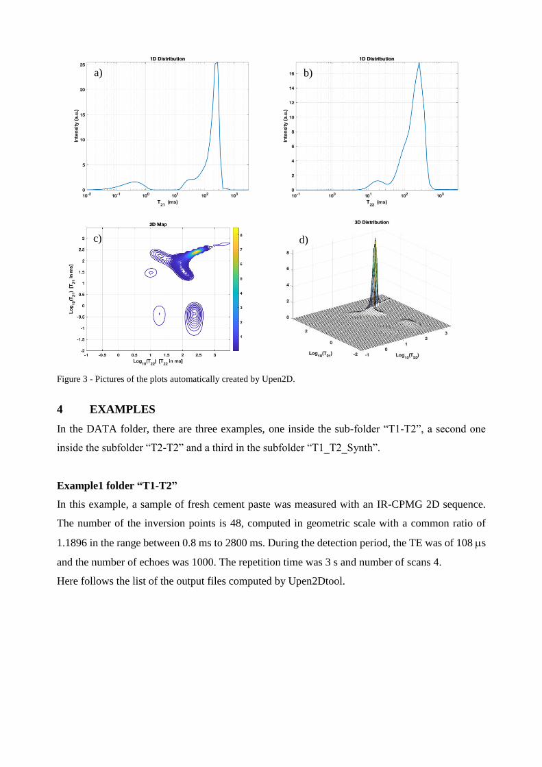
Figure 3 - Pictures of the plots automatically created by Upen2D.

4 EXAMPLES

In the DATA folder, there are three examples, one inside the sub-folder “T1-T2”, a second one

inside the subfolder “T2-T2” and a third in the subfolder “T1_T2_Synth”.

Example1 folder “T1-T2”

In this example, a sample of fresh cement paste was measured with an IR-CPMG 2D sequence.

The number of the inversion points is 48, computed in geometric scale with a common ratio of

1.1896 in the range between 0.8 ms to 2800 ms. During the detection period, the TE was of 108 s

and the number of echoes was 1000. The repetition time was 3 s and number of scans 4.

Here follows the list of the output files computed by Upen2Dtool.

a) b)

c) d)

Figure 4 – “T1-T2” experiment. Projection along the T1 (a) and T2 (b) dimension, (c) Reconstructed 2D Contour

relaxation map, (d) 3D map.

Example2 folder T2-T2

In this example a sample of Maastricht stone saturated with water was measured with a CPMG-

CPMG 2D sequence. During the preparation period, the echo time (TE) was 6.61 ms and the

number of echoes was 128. The mixing time lasts 100 s. During the detection period, the TE was

of 300 s and the number of echoes was 2800. The repetition time was 3 s and number of scans 16.

The output files plots are those reported in the Figure 3 of the paragraph “Output files”.

Example3 folder “T2-T2_Synth”

This is a T1-T2 synthetic case. We consider a reference map distribution of size 64x64 and use it

to synthesize the simulated IR-CPMG data sequence with 1282048 non uniformly distributed

times in the interval [10-3, 3 103] ms. The reference map distribution has the following three

peaks:

Height T1 (ms) T2 (ms)

P1 184.07 807.91 24.95

P2 227.55 6.56 2.48

P3 48.87 572.83 24.95

a) b)

c) d)

The noisy data s are obtained by adding Gaussian white noise of level 10-2 (SNR 20 dB) to the

synthetic data.

The peaks positions and height, computed by 2DUpenTool, are reported in the following table:

Height T1 (ms) T2 (ms)

P1 176.84 959.47 24.95

P2 219.6 6.56 2.46

P3 42.17 572.83 24.95

The Relative Error (Err) and Root Mean Squared Error (RMSE) have the following values:

Err = 0.113, RMSE= 1.720. The computed plots are shown in Figure 5.

Figure 5 - “T1-T2_synth” example. Projection along the (a) T1 and (b) T2 dimension, red line (true relaxation time

distribution), blue line (computed relaxation time distribution), (c) Reconstructed 2D Contour relaxation map, (d) 3D

map.

5 REFERENCES

[1] V. Bortolotti, R. J. S. Brown, P. Fantazzini, G. Landi, F. Zama, Inverse Problems 33 (1) (2016).

[2] B. Blümich, Essential NMR, Springer-Verlag, 2005.

[3] V. Bortolotti, L. Brizi, P. Fantazzini, G. Landi, F. Zama, Filtering techniques for efficient inversion of

two-dimensional nuclear magnetic resonance data, Journal of Physics: Conference Series 904 (1) (2017).

[4] V. Bortolotti, R.J.S. Brown, P. Fantazzini, G. Landi, F. Zama, UPEN2D: Improved 2DUPEN algorithm

for inversion of two-dimensional NMR data, Microporous and Mesoporous Materials 269 195 – 198

(2018).

a) b)

c) d)