Embed Size (px)
Citation preview

A SHORT COURSE ON WITTEN
HELFFER-SJOSTRAND THEORY
D. Burghelea (Ohio State University)
Abstract.
Witten-Helffer-Sjostrand theory is an addition to Morse theory and Hodge-de
Rham theory for Riemannian manifolds and considerably improves on them by in-
jecting some spectral theory of elliptic operators. It can serve as a general tool toprove results about comparison of numerical invariants associated to compact man-
ifolds analytically, i.e. by using a Riemannian metric, or combinatorially, i.e. byusing a triangulation. It can be also refined to provide an alternative presentationof Novikov Morse theory and improve on it in many respects. In particular it can
be used in symplectic topology and in dynamics. This material represents my Notesfor a three lectures course given at the Goettingen summer school on groups and
geometry, June 2000.
Contents
0. Introduction
1. Lecture 1: Morse theory revisited
a. Generalized triangulations
b. Morse Bott generalized triangulations
c. G-generalized triangulations
d. Proof of Theorem 1.1
e. Appendix : The transversality of the maps p and s from
section d.
2. Lecture 2: Witten deformation and the spectral properties of
the Witten Laplacian
a. De Rham theory and integration
Supported in part by NSF
Typeset by AMS-TEX
1

2 WITTEN HELFFER SJOSTRAND THEORY
b. Witten deformation and Witten Laplacians
c. Spectral gap theorems
d. Applications
e. Sketch of the proof of Theorem 2.1
3. Lecture 3: Helffer Sjostrand Theorem, on an asymptotic im-
provement of the Hodge-de Rham theorem
a. Hodge de Rham Theorem
b. Helffer Sjostrand Theorem (Theorem 3.1)
c. Extensions and a survey of other applications
References.
0. Introduction.
Witten Helffer Sjostrand theory, or abbreviated, WHS -theory, consists of anumber of results which considerably improve on Morse theory and De Rham -Hodge theory.
The intuition behind the WHS -theory is provided by physics and consists inregarding a compact smooth manifold equipped with a Riemannian metric and aMorse function (or closed 1-form) as an interacting system of harmonic oscillators.This intuition was first exploited by E. Witten, cf[Wi], in order to provide a short”physicist’s proof ” of Morse inequalities, a rather simple but very useful result intopology.
Helffer and Sjostrand have completed Witten’s picture with their results onSchrodinger operators and have considerably strengthened Witten’s mathemati-cal statements, cf [HS2]. The work of Helffer and Sjostrand on the Witten theorycan be substantially simplified by using simple observations more or less familiarto topologists, cf [BZ] and [BFKM].
The mathematics behind the WHS-theory is almost entirely based on the fol-lowing two facts: the existence of a gap in the spectrum of the Witten Laplacians(a one parameter family of deformed Laplace-Beltrami operator involving a Morsefunction h), detected by elementary mini-max characterization of the spectrum ofselfadjoint positive operators and simple estimates involving the equations of theharmonic oscillator. The Witten Laplacians in the neighborhood of critical pointsin “ admissible coordinates” are given by such equations. The simplification we

D. BURGHELEA 3
referred to are due to a compactification theorem for the space of trajectories andof the unstable sets of the gradient of a Morse function with respect to a ”good”Riemannian metric. This theorem can be regarded as a strengthening of the basicresults of elementary Morse theory.
The theory, initially considered for a Morse function, can be easily extendedto a Morse closed one form, and even to the more general case of a Morse-Bottform.These are closed 1-forms which in some neighborhood of a connected com-ponent of the zero set are differential of a Morse-Bott function. So far the theoryhas been very useful to obtain an alternative derivation of results concerning thecomparison of numerical invariants associated to compact manifolds analytically(i.e. by using a Riemannian metric,) and combinatorially cf[BZ1], [BZ2], [BFKM],[BFK1], [BFK4], [BFKM], [BH].
The theory provides an alternative (analytic) approach to the Novikov- Morsetheory with considerable improvements and consequently has applications in sym-plectic topology and dynamics. These aspects will be developed in a forthcomingpaper [BH].
This minicourse is presented as a series of three lectures. The first is a reconsid-eration of elementary Morse theory, with the sketch of the proof of the compact-ification theorem. The second discusses the ”Witten deformation” of the LaplaceBeltrami operator and its implications and provides a sketch of the proof of Theorem2.1 the main result of the section. The third presents Helffer-Sjostrand Theoremas an asymptotic improvement of the Hodge-de Rham Theorem and finally surveyssome of the existing applications. Part of the material presented in these notes willcontained in a book [BFK5] in preparation, which will be written in collaborationwith L. Friedlander and T. Kappeler.
Lecture 1: Morse Theory revisited.
a. Generalized triangulations.
Let Mn be a compact closed smooth manifold of dimension n. A generalizedtriangulation is provided by a pair (h, g), h : M → R a smooth function, g aRiemannian metric so that
C1. For any critical point x of h there exists a coordinate chart in the neigh-borhood of x so that in these coordinates h is quadratic and g is Euclidean.
More precisely, for any critical point x of h, (x ∈ Cr(h)), there exists a coordinatechart ϕ : (U, x)→ (Dε, 0), U an open neighborhood of x in M, Dε an open disc of

4 WITTEN HELFFER SJOSTRAND THEORY
radius ε in Rn, ϕ a diffeomorphism with ϕ(x) = 0, so that :
(i) h · ϕ−1(x1, x2, · · · , xn) = c− 1/2(x21 + · · ·x2
k) + 1/2(x2k+1 + · · ·x2
n)
(ii) (ϕ−1)∗(g) is given by gij(x1, x2, · · · , xn) = δij
Coordinates so that (i) and (ii) hold are called admissible.It follows then that any critical point x ∈ Cr(h) has a well defined index, i(x) =
index(x) = k, k the number of the negative squares in the expression (i), which isindependent of the choice of a coordinate system (with respect to which h has theform (i)).
Consider the vector field −gradg(h) and for any y ∈M, denote by γy(t),−∞ <t <∞, the unique trajectory of −gradg(h) which satisfies the condition γy(0) = y.For x ∈ Cr(h) denote by W−x resp. W+
x the sets
W±x = y ∈M | limt→±∞
γy(t) = x.
In view of (i), (ii) and of the theorem of existence, unicity and smooth dependenceon the initial condition for the solutions of ordinary differential equations, W−xresp. W+
x is a smooth submanifold diffeomorphic to Rk resp. to Rn−k, with k =index(x). This can be verified easily based on the fact that
ϕ(W−x ∩ Ux) = (x1, x2, · · · , xn) ∈ D(ε)|xk+1 = xk+2 = · · · = xn = 0,
andϕ(W+
x ∩ Ux) = (x1, x2, · · · , xn) ∈ D(ε)|x1 = x2 = · · · = xk = 0.
Since M is compact and C1 holds, the set Cr(h) is finite and since M is closed(i.e. compact and without boundary), M =
⋃x∈Cr(h)W
−x . As already observed
each W−x is a smooth submanifold diffeomorphic to Rk, k =index(x), i.e. an opencell.
C2. The vector field −gradgh satisfies the Morse-Smale condition if for anyx, y ∈ Cr(h), W−x and W+
y are transversal.C2 implies thatM(x, y) := W−x ∩W+
y is a smooth manifold of dimension equal toindex(x)−index(y).M(x, y) is equipped with the action µ : R×M(x, y)→M(x, y),defined by µ(t, z) = γz(t).
If index(x) ≤ index(y), and x 6= y, in view of the transversality requested by theMorse Smale condition, M(x, y) = ∅.
If x 6= y and M(x, y) 6= ∅, the action µ is free and we denote the quotientM(x, y)/R by T (x, y); T (x, y) is a smooth manifold of dimension index(x) ≤index(y)−1, diffeomorphic to the submanifoldM(x, y)∩h−1(λ), for any real numberλ in the open interval (index x, index y). The elements of T (x, y) are the trajectoriesfrom “x to y” and such a trajectory will usually be denoted by γ.

D. BURGHELEA 5
If x = y, then W−x ∩W+x = x.
Further the condition C2 implies that the partition of M into open cells is actu-ally a smooth cell complex. To formulate this fact precisely we recall that ann−dimensional manifold X with corners is a paracompact Hausdorff space equippedwith a maximal smooth atlas with charts ϕ : U → ϕ(U) ⊆ R
n+ with R
n+ =
(x1, x2, · · ·xn)|xi ≥ 0. The collection of points of X which correspond (by someand then by any chart) to points in Rn with exactly k coordinates equal to zerois a well defined subset of X and it will be denoted by Xk. It has a structure of asmooth (n − k)−dimensional manifold. ∂X = X1 ∪X2 ∪ · · ·Xn is a closed subsetwhich is a topological manifold and (X, ∂X) is a topological manifold with bound-ary ∂X. A compact smooth manifold with corners, X, with interior diffeomorphicto the Euclidean space, will be called a compact smooth cell.
For any string of critical points x = y0, y1, · · · , yk with
index(y0) > index(y1) >, · · · , > index(yk),
consider the smooth manifold of dimension index y0 − k,
T (y0, y1)× · · · T (yk−1, yk)×W−yk ,
and the smooth map
iy0,y1,··· ,yk : T (y0, y1)× · · · × T (yk−1, yk)×W−yk →M,
defined by iy0,y1,··· ,yk(γ1, · · · , γk, y) := iyk(y), where ix : W−x → M denotes theinclusion of W−x in M.
Theorem 1.1. Let τ = (h, g) be a generalized triangulation.1)For any critical point x ∈ Cr(h) the smooth manifold W−x has a canonical
compactification W−x to a compact manifold with corners and the inclusion ix hasa smooth extension ix : W−x →M so that :(a) (W−x )k =
⊔(x,y1,··· ,yk) T (x, y1)× · · · × T (yk−1, yk)×W−yk ,
(b) the restriction of ix to T (x, y1)× · · · × T (yk−1, yk)×W−yk is given byix,y1··· ,yk .
2) For any two critical points x, y with i(x) > i(y) the smooth manifold T (x, y)has a canonical compactification T (x, y) to a compact manifold with corners andT (x, y)k =
⊔(x,y1,··· ,yk=y) T (x, y1)× · · · × T (yk−1, yk).
The proof of Theorem 1.1 will be sketched in the last subsection of this section.This theorem was probably well known to experts before it was formulated by
Floer in the framework of infinite dimensional Morse theory cf. [F]. As formulated,

6 WITTEN HELFFER SJOSTRAND THEORY
Theorem 1.1 is stated in [AB]. The proof sketched in [AB] is excessively compli-cated and incomplete. A considerably simpler proof will be sketched in Lecture 1subsection d) and is contained in [BFK5] and [BH].
Observation:O1: The name of generalized triangulation for τ = (h, g) is justified by the
fact that any simplicial smooth triangulation can be obtained as a generalizedtriangulation, cf [Po].
O2: Given a Morse function h and a Riemannian metric g, one can performarbitrary small C0− perturbations of g, so that the pair consisting of h and theperturbed metric is a generalized triangulation, cf [Sm] and [BFK5].
Given a generalized triangulation τ = (h, g), and for any critical point x ∈ Cr(h)an orientation Ox of W−x , one can associate a cochain complex of vector spacesover the field K of real or complex numbers, (C∗(M, τ), ∂∗). Denote the collectionof these orientations by o. The differential ∂∗ depends on the chosen orientationso := Ox|x ∈ Cr(h). To describe this complex we introduce the incidence numbers
Iq : Cr(h)q × Cr(h)q−1 → Z
defined as follows:If T (x, y) = ∅, we put Iq(x, y) = 0.If T (x, y) 6= ∅, for any γ ∈ T (x, y), the set γ×W−y is an open subset of the boundary∂W−x and the orientation Ox induces an orientation on it. If this is the same as theorientation Oy, we set ε(γ) = +1, otherwise we set ε(γ) = −1. Define Iq(x, y) by
Iq(x, y) =∑
γ∈T (x,y)
ε(γ).
In the case M is an oriented manifold, the orientation of M and the orientation Oxon W−x induce an orientation O+
x on the stable manifold W+x .
For any c in the open interval (h(y), h(x)), h−1(c) carries a canonical orientationinduced from the orientation of M. One can check that Iq(x, y) is the intersectionnumber of W−x ∩ h−1(c) with W+
y ∩ h−1(c) inside h−1(c) and is also the incidencenumber of the open cells W−x and W−y in the CW− complex structure provided byτ.
Denote by (C∗(M, τ), ∂∗(τ,o)) the cochain complex of K− Euclidean vector spacesdefined by(1) Cq(M, τ) := Maps(Crq(h),K)(2) ∂q−1
(τ,o) : Cq−1(M, τ)→ Cq(M, τ), (∂q−1f)(x) =∑y∈Crq−1(h) Iq(x, y)f(y),
where x ∈ Crq(h).(3) Since Cq(M, τ) is equipped with a canonical base provided by the maps Exdefined by Ex(y) = δx,y, x, y ∈ Crq(h), it carries a natural scalar product whichmakes Ex, x ∈ Crq(h), orthonormal.

D. BURGHELEA 7
Proposition 1.2. For any q, ∂q · ∂q−1 = 0.
A geometric proof of this Proposition follows from Theorem 1.1. The reader canalso derive it by observing that (C∗(M, τ), ∂∗) as defined is nothing but the cochaincomplex associated to the CW−complex structure provided by τ via Theorem 1.1.
b. Morse Bott generalized triangulations.The concept of generalized triangulation and Theorem 1.1 above can be extended
to pairs (h, g) with h a Morse Bott function; i.e Cr(h) consists of a disjoint unionof compact connected smooth submanifolds Σ and the Hessian of h at any x ∈ Σis nondegenerated in the normal directions of Σ. More precisely a MB-generalizedtriangulation is a pair τ = (h, g) which satisfies C’1 and C’2 below:
C’1: Cr(h) is a disjoint union of closed connected submanifolds Σ, and for anyΣ there the exist admissible coordinates in some neighborhood of Σ. An admissiblecoordinate chart around Σ is provided by:
1) two orthogonal vector bundles ν± over Σ equipped with scalar product pre-serving connections (parallel transports)∇± so that ν+ ⊕ ν− is isomorphic to thenormal bundle of Σ,
2) a closed tubular neighborhood of Σ, ϕ : (U,Σ)→ (Dε(ν− ⊕ ν−),Σ), U closedneighborhood of Σ, so that :
(i) : h · ϕ−1(v1, v2) = c− 1/2||v1||2 + 1/2||v2||2 where v± ∈ E(ν±);(ii) : (ϕ−1)∗(g) is the metric induced from the restriction of g on Σ, the scalar
products and the connections in ν±.
The rank of ν− will be called the index of Σ and denoted by i(Σ) = index(Σ).As before for any x ∈ Cr(h) consider W±x and introduce W±Σ = ∪x∈ΣW
±x .
C’2:(the Morse Smale condition) For any two critical manifolds Σ,Σ′ and x ∈ Σ,W−x and W+
Σ′ are transversal.As before C’2 implies thatM(Σ,Σ′) := W−Σ ∩W
+Σ′ is a smooth manifold of dimen-
sion equal to i(Σ)−i(Σ′)−dim Σ, and that the evaluation maps u :M(Σ,Σ′)→ Σ isa smooth bundle with fiber W−x ∩W+
Σ′ a smooth manifold of dimension i(Σ)− i(Σ′).M(Σ,Σ′) is equipped with the free action µ : R×M(Σ,Σ′)→M(Σ,Σ′) defined
by µ(t, z) = γz(t) and we denote the quotient space M(Σ,Σ′)/R by T (Σ,Σ′).T (Σ,Σ′) is a smooth manifold of dimension i(Σ) − i(Σ′)+dim Σ−1, diffeomorphicto the submanifold M(Σ,Σ′) ∩ h−1(λ), for any real number λ in the open interval(h(Σ), h(Σ′)). In addition, one has the evaluation maps, uΣ,Σ′ : T (Σ,Σ′) → Σwhich is a smooth bundle with fiber W−x ∩W+
Σ′/R, a smooth manifold of dimensioni(Σ) − i(Σ′) − 1, and lΣ,Σ′ : T (Σ,Σ′) → Σ′ a smooth map. The maps u··· and l···induce by pull- back constructions the smooth bundles
u(Σ0,Σ1,··· ,Σk) : T (Σ0,Σ1)×Σ1 · · · ×Σk−1 T (Σk−1,Σk)→ Σ0,

8 WITTEN HELFFER SJOSTRAND THEORY
the smooth maps
l(Σ0,Σ1,··· ,Σk) : T (Σ0,Σ1)×Σ1 · · · ×Σk−1 T (Σk−1,Σk)→ Σk
and
iΣ0,Σ1,··· ,Σk : T (Σ0,Σ1)×Σ1 · · · ×Σk−1 T (Σk−1,Σk)×Σk W−Σk→M,
defined by iΣ0,y1,··· ,yk(γ1, · · · , γk, y) := iΣk(y), for γi ∈ T (Σi−1,Σi) and y ∈W−Σk ,The analogue of Theorem 1.1 is Theorem 1.1’ below. The proof of Theorem 1.1
as given below, subsection d), and is formulated in such way that the extension tothe Morse Bott case is straightforward.
Theorem 1.1’.Let τ = (h, g) be a MB generalized triangulation.1) For any critical manifold Σ ⊂ Cr(h), the smooth manifold W−Σ has a canonical
compactification to a compact manifold with corners W−Σ , and the smooth bundleπ−Σ : W−Σ → Σ resp. the smooth inclusion iΣ : W−Σ → M have extensions π−Σ :W−Σ → Σ, a smooth bundle whose fibers are compact manifolds with corners, resp.iΣ : W−Σ →M a smooth map, so that
(a): (W−Σ )k =⊔
(Σ,Σ1,··· ,Σk) T (Σ,Σ1)×Σ1 · · · ×Σk−1 T (Σk−1,Σk)×Σk W−Σk,
(b): the restriction of iΣ to T (Σ,Σ1)×Σ1 · · · ×Σk−1 T (Σk−1,Σk)×Σk W−Σk
is givenby iΣ,Σ1··· ,Σk .
2) For any two critical manifolds Σ,Σ′ with i(Σ) > i(Σ′) the smooth mani-fold T (Σ,Σ′) has a canonical compactification to a compact manifold with cornersT (Σ,Σ′) and the smooth maps u : T (Σ,Σ′)→ Σ and l : T (Σ,Σ′)→ Σ′ have smoothextensions u : T (Σ,Σ′) → Σ and l : T (Σ,Σ′) → Σ′ with u a smooth bundle whosefibers are compact manifolds with corners. Precisely
(T (Σ,Σ′))k =⊔
(Σ,Σ1,··· ,Σk) T (Σ,Σ1)×Σ1 · · · ×Σk−1 T (Σk−1,Σk).
For a critical manifold Σ choose an orientation of ν− if this bundle is orientableand an orientation of the orientable double cover of ν− if not. Such an object will bedenoted byOΣ and the collection of allOΣ will be denoted by o ≡ OΣ|Σ ⊂ Cr(h).
Choosing the collection o in addition to the Morse-Bott generalized triangulationτ one can provide as an analogue of the geometric complex (C∗(M, τ), ∂∗(τ,o)) thecomplex (C∗, D∗) defined by
Cr =:⊕
(k,Σ)|k+i(Σ)=r
Ωk(Σ, o(ν−))
and Dr : Cr → Cr+1 given by the matrix |||∂kΣ,Σ′ ||| whose entries

D. BURGHELEA 9
∂k(Σ,Σ′) : Ωk(Σ′, o(ν′−))→ Ωr−i(Σ)+i(Σ′)+1(Σ, o(ν−)) are given by1
∂k(Σ,Σ′) =
dk : Ωk(Σ, o(ν−))→ Ωk+1(Σ, o(ν−))if Σ = Σ′
(−1)k(uΣ,Σ′)∗ · (lΣ,Σ′)∗otherwise
Here Ω∗(Σ, o(ν−)) denotes the differential forms on Σ with coefficients in the
orientation bundle of ν− and (...)∗ denotes the integration along the fiber of uΣ,Σ′ .
The orientation bundle of ν− has a canonical flat connection. When ν− is ori-entable then this bundle is trivial as bundle with connection and Ω∗ identifies tothe ordinary differential forms.
A Morse Bott function h is a smooth function for which the critical set consistsof a disjoint union of connected manifolds Σ, so that the Hessian of h at each criticalpoint of Σ is nondegenerated in the normal direction.
Observation:O.2’: Given a pair (h, g) with h a Morse Bott function and g is a Riemannian
metric one can provide arbitrary small C0 perturbation g′ of g so that the pair(h, g′) satisfies C ′. If (h, g) satisfies C ′1 one can choose g′ arbitrary closed to g inC0−topology so that g = g′ away from a given neighborhood of the critical pointset, g′ = g in some (smaller) neighborhood of the critical point set and (h, g′) is anMB generalized triangulation.
c. G-Generalized triangulations.
Of particular interest is the case of a smooth G−manifold (M,µ : G×M →M)where G is a compact Lie group and µ a smooth action. In this case we considerpairs (h, g) with h a G-invariant smooth function and g a G−invariant Riemannianmetric. Then Cr(h) consists of a union of G−orbits. The G−version of conditionsC1 and C2 are obvious to formulate. We say that the pair (h, g) with both hand g G−invariant is a G-generalized triangulation resp. normal G-generalizedtriangulation if G-C1 (resp. normal G-C1) and G-C2 hold.
G-C1: Cr(h) is a finite union of orbits denoted by Σ and for any critical orbitΣ we require the existence of an admissible chart. More precisely, such a chartaround Σ is provided by the following data:
1: A closed subgroup H ⊂ G, two orthogonal representations ρ± : H → O(V±)and a scalar product on the Lie algebra g of G which is invariant with respect tothe adjoint representation restricted to H.ρ± induce orthogonal bundles ν± : E(ν±) → Σ. The total space of these G−
bundles are E(ν±) = G×H V±. The scalar product on g and the the scalar product
1this formula is implicit in (2.2) in view of the fact that Int∗ : (Ω∗, d∗) → (C∗(M, τ), ∂∗) issupposed to be a surjective morphism of cochain complexes

10 WITTEN HELFFER SJOSTRAND THEORY
on V = V− ⊕ V+ induces a G−invariant Riemannian metric on G and on G × V.The metric on G×V descends to a G−invariant Riemannian metric on E(ν−⊕ν+).
2) A positive number ε, a constant c ∈ R and a G−equivariant diffeomorphismϕ : (U,Σ) → Dε(ρ+ ⊕ ρ−) where U is a closed G− tubular neighborhood of Σ inM, and Dε denotes the disc of of radius ε in the underlying Euclidean space of therepresentation ρ+ ⊕ ρ−, so that
(i) : h · ϕ−1((g, v1, v2)) = c− 1/2||v1||2 + 1/2||v2||2) where v± ∈ E(ν±)(ii) : (ϕ−1)∗(g) is the Riemannian metric on E(ν− ⊕ ν+) described above.We call the admissible chart ”normal” if in addition ρ− is trivial. The condition
normal G-C1 requires the admissible charts to be normal.G-C2: This condition is the same as C’2.Observation:O1”: Given a pair (h, g) one can perform an arbitrary small C0 perturbation
(h′, g′) so that (h′, g′) satisfies normal G-C1. This was proven in [M].O2”: Given (h, g) a pair which satisfies normal G-C1 then one can perform an
arbitrary small C0 perturbation on the metric g and obtain the G− invariant metricg′ (away from the critical set) so that (h, g′) satisfies G-C2. This result is provenin [B].
Clearly, aG−generalized triangulation is aMB−generalized triangulation, henceTheorem 1.1’ above can be restated in this case as Theorem 1.1” with the additionalspecifications that in the statement of Theorem 1.1’ all compact manifolds withcorners are G− manifolds and all maps are G− equivariant.
Note that a G−generalized triangulation provides via Theorem 1.1” a structureof a smooth G−handle body and a normal G− generalized triangulation providesa structure of smooth G−CW complex for M. The smooth triangulability of com-pact smooth manifolds with corners if combined with the existence of normal G−generalized triangulation lead to the existence of a smooth G−triangulation in thesense of [I] and then to the existence of smooth triangulation of the orbit spacesof a smooth G−manifold when G is compact. There is no proof for this result inliterature. The best known result so far, is the existence of a C0 triangulation ofthe orbit space established by Verona. [V].
d): Proof of Theorem 1.1.
Some notationsWe begin by introducing some notations:
Let c0 < c1 · · · < cN be the collection of all critical values (c0 the absolute minimum,cN the absolute maximum) and fix ε > 0 small enough so that ci − ε > ci−1 + ε forall i ≥ 1. Denote by:
Cr(i) := Cr(h) ∩ h−1(ci),

D. BURGHELEA 11
Mi := h−1(ci),
M±i := h−1(ci ± ε)
M(i) := h−1(ci−1, ci+1)
For any x ∈ Cr(i) denote by:
S±x := W±x ∩ M±i
Sx := S+x × S−x
W±x (i) := W±x ∩M(i)
SW x(i) := S+x ×W−x (i).
It will be convenient to write
S±i :=⋃
x∈Cr(i)
S±x
Si :=⋃
x∈Cr(i)
Sx ⊂M−i ×M+i
W±(i) :=⋃
x∈Cr(i)
W±x (i)
SW (i) :=⋃
x∈Cr(i)
S+x ×W−x (i)

12 WITTEN HELFFER SJOSTRAND THEORY
Observe that:1) Si ⊂M+
i ×M−i , SW (i) ⊂M+
i ×M(i)2) M±i is a smooth manifold of dimension n − 1, (n = dimM) and M(i) is a
smooth manifold of dimension n, actually an open set in M. Mi is not a mani-
fold, however,M i := Mi \ Cr(i),
M±
i := M±i \ S±i are are smooth manifolds
(submanifolds of M) of dimension n− 1.
The flow Φt and few induced mapsLet Φt be the flow associated to the vector field −gradgh/|| − gradgh|| on
M \ Cr(h) and consider:a) the diffeomorphisms
ψi : M−i →M+i−1
ϕ±i :
M±i →M i
obtained by the restriction of Φ(ci−ci−1−2ε) and Φ±ε,
b) the submersion ϕ(i) : M(i) \ (W−(i) ∪W+(i)) →M i defined by ϕ(i)(x) :=
Φh(x)−ci(x).Observe that ϕ±i and ϕ(i) extend in an unique way to continuous maps
ϕ±i : M±i →M, ϕ(i) : M(i)→Mi.
Two manifolds with boundary
The manifold Pi : Define
Pi := (x, y) ∈M−i ×M+i | ϕ
−i (x) = ϕ+
i (y),

D. BURGHELEA 13
and denote by p±i : Pi →M±i the canonical projections. One can verify that Pi is acompact smooth (n−1) dimensional manifold with boundary, (smooth submanifoldof M−i ×M
+i ) whose boundary ∂Pi can be identified to Si ⊂M−i ×M
+i . Precisely
OP1: p±i : Pi \ ∂Pi →M±
i are diffeomorphisms,OP2: the restriction of p+
i × p−i to ∂Pi is a diffeomorphism onto Si. (Each p±i
restricted to ∂Pi is the projection onto S±i .)
The manifold Q(i) : Define
Q(i) = (x, y) ∈M+i ×M(i)|ϕ+
i (x) = ϕ(i)(y)
or equivalently, Q(i) consists of pairs of points (x, y), x ∈ M+i , y ∈ M(i) which
lie on the same (possibly broken) trajectory and denote by li : Q(i) → M+i resp.
ri : Q(i)→M(i) the canonical projections.One can verify that Q(i) is a smooth n−dimensional manifold with boundary,
(smooth submanifold of M+i ×M(i)) whose boundary ∂Q(i) is diffeomorphic to
SW (i) ⊂M+i ×M(i). More precisely
OQ1: li : Q(i) \ ∂Q(i) →M
+
i is a smooth bundle with fiber an open segmentand ri : Q(i) \ ∂Q(i)→M(i) \W−(i) a diffeomorphism,
OQ2: the restriction of l × r to ∂Q(i) is a diffeomorphism onto SW (i). (l resp.r restricted to ∂Q(i) identifies with the projection onto S+
i resp. W (i)).
Since Pi and Q(i) are smooth manifolds with boundaries,
Pr,r−k := Pr × Pr−1 · · ·Pr−k
andPr(r − k) := Pr × · · ·Pr−k+1 ×Q(r − k)
are smooth manifolds with corners.Our arguments for the proof of Theorem 1.1 will be based on the following
method for recognizing a smooth manifold with corners. If P is a smooth manifoldwith corners, O,S smooth manifolds, p : P → O and s : S → O smooth maps sothat p and s are transversal (p is transversal to s if its restriction to each k− cornerof P is transversal to s, ) then p−1(s(S)) is a smooth submanifold with corners ofP.
Proof of Theorem 1.1 First we prove part (2). We want to verify thatT (x, y) (cf the definition in the statement of Theorem 1.1) is a smooth manifoldwith corners. Let x ∈ Cr(r + 1) and y ∈ Cr(r − k − 1), k ≥ −2. If k = −2 thestatement is empty, if k = −1 there is nothing to check, so we suppose k ≥ 0.
We consider P = Pr,k as defined above, O =∏r−kr (M+
i × M−i )), and S =S−x ×M−r · · · ×M−(r−k+1) × S
+y . In order to define the maps p and s we consider

14 WITTEN HELFFER SJOSTRAND THEORY
ωi : M−i →M−i ×M+i+1 given by ωi(x) = (x, ψi(x)), and
pi : Pi →M+i ×M
−i given by pi(y) = (p+
i (y), p−i (y)).We also denote by α : S−x → M+
r and β : S+y → M−k−r the restriction of ψr+1
resp. of ψ−1r−k to S−x resp. S+
y . Take s = α× ωr · · ·ωr−k+1 × β and p :=∏r−ki=r πi.
The verification of the transversality follows easily from OP1, OP2 and the MorseSmale condition C2. It is easy to see that p−1(s(S)) is compact and identifies toT (x, y); the verification of this fact is left to the reader.
To prove part (1) we first consider the map ix : X = W−x →M defined by (a) and(b) in Theorem 1.1 (1). Let X := W−x and for any positive integer k we denote byX(k) := i−1
x (M(k)). The proof will be given in two steps. First we will topologizeX(k) and put on it a structure of a smooth manifold with corners, so that therestriction of ix to X(k) is a smooth map. Second we check that X(k) and X(k′)induce on the intersection X(k) ∩X(k′) the same topology and the same smoothstructure. These facts imply that X has a canonical structure of smooth manifoldwith corners and ix is a smooth map. The compacity of X follows by observingthat the image ix(X) is compact and the preimage of any point is compact.
To accomplish the first step we proceed in exactly the same way as in the proofof part (2). Suppose x ∈ Cr(r + 1). ConsiderP := Pr(k),O := (M+
r ×M−r )× · · · (M+r−k+1 ×M
−k+r−1)×M+
r−k, and
S := S−x ×M−r · · · ×M−r−k+1.
Takep := pr × · · · × pr−k+1 × lr−k ands = α× ωr · · · × ωr−k+1.
The verification of the transversality follows from OP1, OP2, OQ1, OQ2 andthe Morse Smale condition C2 above as explained in the Appendix. It is easy tosee that p−1(s(S)) identifies to X(r − k).
The second step is more or less straightforward, so it will be left again to thereader. q.e.d.
Appendix : The verification of transversality of the maps p and s.
Consider the diagrams

D. BURGHELEA 15
S−r+1
α
M−r
id
ψr
6666666M−r−1
id
· · · M−r−k+1
ψr−k+1
<<<<<<<S+r−k−1
β
M+r
222222
M−r M+r−1 M−r−1 · · · M+
r−k M−r−k
Pr
p+r
YY222222p−r
FF Pr−1
p+r−1
[[8888888
p−r−1
CC· · · Pr−k
p+r−k
\\8888888
p−r−kAA
Diagram 1
S−r+1
α
M−r
id
ψr
6666666M−r−1
ψr−k+1· · · M−r−k+1
ψr−k+1
AAAAAAAA
M+r M−r M+
r−1 M−r−1 · · · M+r−k
Pr
p+r
YY2222222p−r
FF Pr−1
p+r−1
[[8888888
p−r−1
CC· · · Q(r − k)
lr−k
OO
Diagram 1’
M−r
id
ψr
6666666M−r−1
id
· · · M−r−k+1
ψr−k+1
<<<<<<<S+r−k−1
β
M−r M+
r−1 M−r−1 · · · M+r−k M−r−k
S−r
i
OO
Pr−1
p−r−1
[[8888888
p+r−1
CC· · · Pr−k
p+r−k
[[8888888
p−r−k
AA
Diagram 2

16 WITTEN HELFFER SJOSTRAND THEORY
S−r+1
α
M−r
id
ψr
6666666M−r−1
id
· · · M−r−k+1
ψr−k+1
<<<<<<<
M+r M−r M+
r−1 M−r−1 · · · M+r−k
Pr
p+r
XX2222222p−r
FFPr−1
p+r−1
[[7777777
p−r−1
CC· · · S+
r−k
i
OO
Diagram 3
M−r
id
ψr
6666666M−r−1
id
· · · M−r−k+1
ψr−k+1
AAAAAAAA
M−r M+r−1 M−r−1 · · · M+
r−k
S−r
i
OO
Pr−1
p+r−1
[[8888888
p−r−1
CC· · · Q(r − k)
lr−k
OO
Diagram 4
For each of these diagrams denote by P resp. O resp. R, the product of themanifolds on the third resp. second resp. first row and let p : P → O resp.s : R → O denote the product of the maps from the third to the second row resp.the first to the second row. Clearly P is a smooth manifold with corners. Denote
byP the interior of P, i.e P \ ∂P, and by
p :P → O the restriction of p to
P.
We refer to the statement ”p transversal to s” with p and s obtained from the
diagram 1, 1’ 2, 2’, 3, 4 as: T 1r,k, T
1′
r,k, T2r,k, T
2′
r,k, T3r,k, T
4r,k.
In view of the observation OP2 and OQ2 and of the fact that ” mi : Mi →Oiandsi : Ri → Oi, i = 1, 2,Mi,Oi,Ri smooth manifolds imply the transversalityof m1 ×m2 :M1 ×M2 → O1 ×O2and s1 × s2 : R1 ×R2 → O1 ×O2”, it is easyto see that the transversality of p and s obtained from the diagram 1 resp. 1′ canbe derived from the validity of the statements T 1
r,k, T2r,k, T
3r,k resp. T 1′
r,k, T3r,k, T
4r,k
for various r, k.In view of the fact that all arrows except α, β, lr−k and the inclusions ( cf Di-
agrams 2,3,4) are open embeddings, the properties T 1r,k, · · · , T 4
r,k follow from thetransversality of W−r+1 and W+
r−k−1. This finishes the verification of the transver-sality statement needed for the proof of Theorem 1.1. q.e.d

D. BURGHELEA 17
Lecture 2: Witten deformation and the spectral properties of the WittenLaplacian.
a. De Rham theory and integration.Let M be a closed smooth manifold and τ = (h, g) be a generalized triangu-
lation or more general a Morse-Bott generalized triangulation and o a system oforientations. Denote by (Ω∗(M), d∗) the De Rham complex of M. This is a cochaincomplex whose component Ωq(M) is the (Frechet) space of smooth differentialforms of degree q and whose differential dq : Ωq(M) → Ωq+1(M) is given by theexterior differential d. Recall that Stokes’ theorem for manifolds with corners canbe formulated as follows:
Theorem. Let P be a compact r−dimensional oriented smooth manifold with cor-ners and f : P → M a smooth map. Denote by ∂f : P1 → M the restriction of fto the smooth oriented manifold P1 (P1 defined as in section 1a). If ω ∈ Ωr−1(M)is a smooth form then
∫P1
(∂f)∗(ω) is convergent and∫P
f∗(dω) =∫P1
(∂f)∗(ω).
Define the linear maps Intq : Ωq(M)→ Cq(M, τ) as follows.a) In the case τ is a generalized triangulation and Cq(M, τ) := Maps(Crq(h),K),
Intq is defined by
Intq(ω)(x) :=∫W−x
ω,(2.1)
where K is the field of real or complex numbers.b) In the case τ is an Morse-Bott generalized triangulation and
Cq(M, τ) :=⊕
k+dim(Σ)=q
Ωk(Σ, o(ν−)),
Intq is given by integrating the pull back by iΣ : W−Σ → M of a form ω ∈ Ωq(M)along the fiber of πΣ : W−Σ → Σ, i.e.
Intq(ω) = ⊕k+dim(Σ)=q(π−Σ )∗i∗Σω ∈ Ωq−i(Σ)(Σ, o(ν−))(2.2)
It is a consequence of Theorem 1.1 (1.1’) that the collection of the linear mapsIntq defines a morphism
Int∗ : (Ω∗(M), d∗)→ (C∗(M, τ), ∂∗)
of cochain complexes which has the following property (de Rham):

18 WITTEN HELFFER SJOSTRAND THEORY
Theorem. Int∗ induces an isomorphism in cohomology.
c) Suppose that we are in the case of a G−manifold and τ is a G−generalizedtriangulation as described in section 1. Fix an irreducible representation ξ : G →O(Vξ) and denote by (Ω∗ξ , d
∗ξ) resp. (C∗ξ , ∂
∗ξ ) the subcomplex of (Ω∗, d∗) resp.
(C∗, ∂∗) defined by the property that Ω∗ξ resp. C∗ξ is the largest G−invariant sub-space of Ω∗ resp. C∗ which contains no other irreducible representation but ξ.Equivalently for any irreducible representation ξ′, ξ′ 6= ξ, Ω∗ξ ⊗G Vξ′ = 0 resp.C∗ξ ⊗G Vξ′ = 0. Since G is compact, (Ω∗, d∗) = ⊕ξ(Ω∗ξ , d∗ξ) resp. (C∗, ∂∗) =⊕ξ(C∗ξ , ∂∗ξ ). Since the integration map is G−equivariant, Int(Ω∗ξ) ⊂ C∗ξ .
Denote byInt∗ξ : (Ω∗ξ , d
∗ξ)→ (C∗ξ , ∂
∗ξ )
the restriction of Int∗ to the components (Ω∗ξ , d∗ξ) corresponding to ξ.
We have the following refinement of de Rham Theorem.
Theorem. Int∗ξ induces an isomorphism in cohomology.
Theorem 3.1-1” below (Lecture 3) will imply these theorems.
b) Witten deformation and Witten Laplacians.
Let M be a closed manifold and α ∈ Ω1(M) a closed 1− form, i.e dα = 0. Fort > 0 consider the complex (Ω∗(M), d∗(t)) with differential
dq(t)(ω) = dω + tα ∧ ω.(2.3)
If α = dh with h : M → R a smooth function, dq(t)(ω) = e−thdeth(ω) and d∗(t)is the unique differential in Ω∗(M) which makes the multiplication by the smoothfunction eth an isomorphism of cochain complexes
eth : (Ω∗(M), d∗(t))→ (Ω∗(M), d∗).
Recall that for any vector field X on M one defines a zero order differentialoperator, ι∗X : Ω∗(M)→ Ω∗−1(M), by
(ιqXω)(X1, X2, · · · , Xq−1) := ω(X,X1, · · · , Xq−1)(2.4)
and a first order differential operator L∗X : Ω∗(M)→ Ω∗(M), the Lie derivative inthe direction X, by
LqX := dq−1 · ιqX + ιq+1X · dq.(2.5)

D. BURGHELEA 19
They satisfy the following identities:
ιX(ω1 ∧ ω2) = ιX(ω1) ∧ ω2 + (−1)|ω1|ω1 ∧ ιX(ω2).(2.6)
where |ω1| denotes the degree of ω1 and
LX(ω1 ∧ ω2) = LX(ω1) ∧ ω2 + ω1 ∧ LX(ω2).(2.7)
Given a Riemannian metric g on the oriented manifold M we have the zero orderoperator Rq : Ωq(M) → Ωn−q(M), known as the Hodge-star operator which, withrespect to an oriented orthonormal frame e1, e2, · · · , en in the cotangent space atx, is given by
Rqx(ei1 ∧ · · · ∧ eiq ) = ε(i1, · · · , iq)e1 ∧ · · · ∧ ei1 ∧ · · · ∧ eiq ∧ · · · ∧ en,(2.8)
where 1 ≤ i1 < i2 < · · · < iq ≤ n, and ε(i1, i2, · · · , iq) denotes the sign of thepermutation of (1, · · · , n) given by
(i1, · · · , iq, 1, 2, · · · , i1, · · · , i2, · · · , i2, · · · , iq, · · · , n).
Here a “hat” above a symbol means the deletion of this symbol.The operators Rq satisfy
Rq ·Rn−q = (−1)q(n−q)Id.(2.9)
With the help of the operators Rq for an oriented Riemannian manifold of dimen-sion n, one defines the fiberwise scalar product , : Ωq(M)×Ωq(M)→ Ω0(M)and the formal adjoints of dq, dq(t), ιqX , L
qX , by the formulas
ω1, ω2 = (Rn)−1(ω1 ∧Rq(ω2)),(2.10)
δq+1 = (−1)nq+1Rn−q · dn−q−1 ·Rq+1 : Ωq+1(M)→ Ωq(M),(2.11)δq+1(t) = (−1)nq+1Rn−q · dn−q−1(t) ·Rq+1 : Ωq+1(M)→ Ωq(M),
(ιqX)] = (−1)nq−1Rn−q · ιn−q−1X ·Rq−1 : Ωq−1(M)→ Ωq(M),
(LqX)] = (−1)(n+1)q+1Rn−q · Ln−qX ·Rq : Ωq(M)→ Ωq(M)
These operators satisfy
ιXω1, ω2 = ω1, (ιX)]ω2 (2.12)
and
(LX)] = (ιX)] · δ + δ · (ιX)].(2.13)

20 WITTEN HELFFER SJOSTRAND THEORY
Note that LqX + (LqX)] is a zeroth order differential operator. Let X] denotethe element in Ω1(M) defined by X](Y ) := X,Y and for α ∈ Ω1(M) let(Eα)q : Ωq(M)→ Ωq+1(M), denote the exterior product by α. Then we have
(ιqX)] = (EX])q−1.(2.14)
It is easy to see that the scalar products, and hence the operators δq, δq(t), ι]Xand L]X are independent of the orientation of M. Therefore they are defined (firstlocally and then, being differential operators, globally) for an arbitrary Riemannianmanifold, not necessarily orientable, and satisfy (2.10), (2.12)-(2.14) above.
For a Riemannian manifold (M, g) one introduces the scalar product Ωq(M) ×Ωq(M)→ C by
< ω,ω′ >:=∫M
ω ∧ ω′ =∫M
ω, ω′ dvol(g).(2.15)
In view of (2.12), δq+1(t), (ιqX)] and (LqX)] are formal adjoints of dq(t), ιqX(t)and LqX with respect to the scalar product < ., . > .
For a Riemannian manifold (M, g), one introduces the second order differentialoperators ∆q : Ωq(M) → Ωq(M), the Laplace Beltrami operator, and ∆q(t) :Ωq(M)→ Ωq(M), the Witten Laplacian (for the 1-form α) by
∆q := δq+1 · dq + dq−1 · δq,
and∆q(t) := δq+1(t) · dq(t) + dq−1(t) · δq(t).
Note that ∆q(0) = ∆q. In view of (2.3) -(2.10) and (2.12) one verifies
∆q(t) = ∆q + t(L−gradgα + L]−gradgα) + t2||α||2Id(2.16)
where gradgα is the unique vector field defined by (gradgα)] = α. One verifies thatL−gradgα + L]−gradgα is a zeroth order differential operator.
The operators ∆q(t) are elliptic, essentially selfadjoint, and positive, hence theirspectra, spect∆q(t), are contained in [0,∞). Further
ker ∆q(t) = ω ∈ Ωq(M)|dq(t) = 0, δq(t) = 0
If α = dh and if 0 is an eigenvalue of ∆q(0), then 0 is an eigenvalue of ∆q(t)for all t and with the same multiplicity: this because dq(t) = e−th · dq · eth· andδq(t) = e−th · δq · eth·.
D. BURGHELEA 21
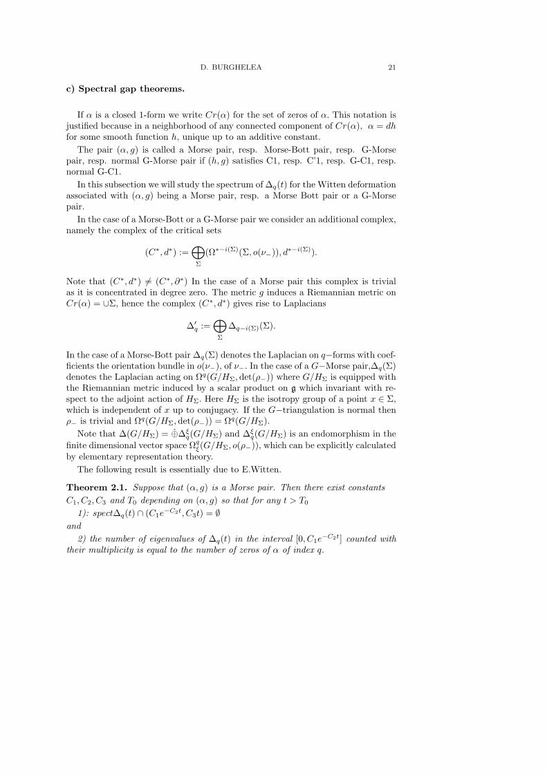
c) Spectral gap theorems.
If α is a closed 1-form we write Cr(α) for the set of zeros of α. This notation isjustified because in a neighborhood of any connected component of Cr(α), α = dhfor some smooth function h, unique up to an additive constant.
The pair (α, g) is called a Morse pair, resp. Morse-Bott pair, resp. G-Morsepair, resp. normal G-Morse pair if (h, g) satisfies C1, resp. C’1, resp. G-C1, resp.normal G-C1.
In this subsection we will study the spectrum of ∆q(t) for the Witten deformationassociated with (α, g) being a Morse pair, resp. a Morse Bott pair or a G-Morsepair.
In the case of a Morse-Bott or a G-Morse pair we consider an additional complex,namely the complex of the critical sets
(C∗, d∗) :=⊕
Σ
(Ω∗−i(Σ)(Σ, o(ν−)), d∗−i(Σ)).
Note that (C∗, d∗) 6= (C∗, ∂∗) In the case of a Morse pair this complex is trivialas it is concentrated in degree zero. The metric g induces a Riemannian metric onCr(α) = ∪Σ, hence the complex (C∗, d∗) gives rise to Laplacians
∆′q :=⊕
Σ
∆q−i(Σ)(Σ).
In the case of a Morse-Bott pair ∆q(Σ) denotes the Laplacian on q−forms with coef-ficients the orientation bundle in o(ν−), of ν−. In the case of a G−Morse pair,∆q(Σ)denotes the Laplacian acting on Ωq(G/HΣ,det(ρ−)) where G/HΣ is equipped withthe Riemannian metric induced by a scalar product on g which invariant with re-spect to the adjoint action of HΣ. Here HΣ is the isotropy group of a point x ∈ Σ,which is independent of x up to conjugacy. If the G−triangulation is normal thenρ− is trivial and Ωq(G/HΣ,det(ρ−)) = Ωq(G/HΣ).
Note that ∆(G/HΣ) = ⊕∆ξq(G/HΣ) and ∆ξ
q(G/HΣ) is an endomorphism in thefinite dimensional vector space Ωqξ(G/HΣ, o(ρ−)), which can be explicitly calculatedby elementary representation theory.
The following result is essentially due to E.Witten.
Theorem 2.1. Suppose that (α, g) is a Morse pair. Then there exist constantsC1, C2, C3 and T0 depending on (α, g) so that for any t > T0
1): spect∆q(t) ∩ (C1e−C2t, C3t) = ∅
and2) the number of eigenvalues of ∆q(t) in the interval [0, C1e
−C2t] counted withtheir multiplicity is equal to the number of zeros of α of index q.

22 WITTEN HELFFER SJOSTRAND THEORY
The above theorem states the existence of a gap in the spectrum of ∆q(t), namelythe open interval (C1e
−C2t, C3t), which widens to (0,∞) when t→∞.Clearly C1, C2, C3 and T0 determine a constant T > T0, so that for t ≥ T, 1 ∈
(C1e−C2t, C3t) and therefore
spect∆q(t) ∩ [0, C1e−C2t] = spect∆q(t) ∩ [0, 1]
andspect∆q(t) ∩ [C3t,∞) = spect∆q(t) ∩ [1,∞).
For t > T we denote by Ωq(M)sm(t) the finite dimensional subspace of Ωq(M)generated by the q−eigenforms of ∆q(t) corresponding to the eigenvalues of ∆q(t)smaller than 1. Note that Ωq(M)sm(t) is of dimension mq where mq is the numberof critical points of index q of the closed 1-form α.
The theory of elliptic operators implies that these eigenforms which are a priorielements in the L2−completion of Ωq(M), are actually smooth, i.e. in Ωq(M). Notethat d(t)(Ωq(M)sm(t)) ⊂ Ωq+1(M)sm(t), so that (Ω∗(M)sm(t), d∗(t)) is a finite di-mensional cochain subcomplex of (Ω∗(M), d∗(t)) and (eth(Ω∗(M)sm(t)), d∗) is afinite dimensional subcomplex of (Ω∗(M), d∗). Clearly the L2−orthogonal comple-ment of Ω∗(M)sm(t) in Ω∗(M) is also a closed Frechet subcomplex (Ω∗(M)la(t), d∗(t))of (Ω∗(M), d∗(t)) and we have the following decomposition
(Ω∗(M), d∗(t)) = (Ω∗(M)sm(t), d∗(t))⊕ (Ω∗(M)la(t), d∗(t))(2.17)
with (Ω∗(M)la(t), d∗(t)) acyclic.Let us consider now the case of a Morse-Bott pair. Denote by λ′q,1 ≤ λ′q,2 ≤
· · · ≤ λ′q,r ≤ · · · be the spectrum of ∆′q, and by λ′q the first nonzero eigenvalue of∆′q. The following result is due to Helffer [H] (cf also [P]).
Theorem 2.1’. Suppose that (α, g) is a Morse-Bott pair and r ≥ 1, an integer.Then there exist positive constants C1, C2, T0, so that for any t > 0 and t ≥ T and1 ≤ q ≤ n|λq,r(t)− λ′q,r| < C1t
−C2 where λq,r(t) is the r−th eigenvalue of ∆q(t).
In particular one can find T ≥ T0 so that for λ′ = infλ′q and t > T
1) Spect∆q(t) ∩ (C1t−C2 ,−C1t
−C2 + λ′) = ∅2) λ′/2 ∈ (C1t
−C2 ,−C1t−C2 + λ′).
Therefore one can again produce a decomposition of the form
(Ω∗(M), d∗(t)) = (Ω∗(M)sm(t), d∗(t))⊕ (Ω∗(M)la(t), d∗(t))(2.17′)
where (Ω∗(M)sm(t), d∗(t)) is a finite dimensional cochain subcomplex of (Ω∗, d∗(t))with (Ωq(M)sm(t) given by the span of the eigenforms corresponding to eigenvalues
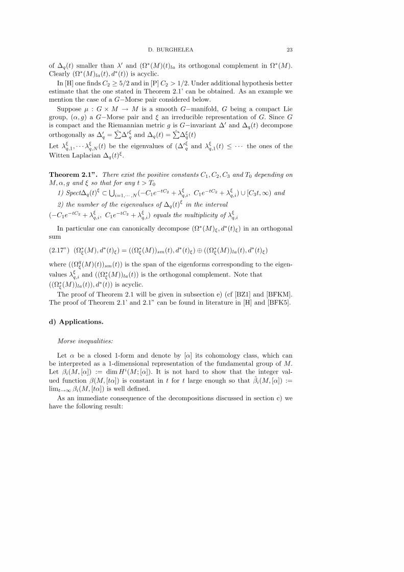
D. BURGHELEA 23
of ∆q(t) smaller than λ′ and (Ω∗(M)(t)la its orthogonal complement in Ω∗(M).Clearly (Ω∗(M)la(t), d∗(t)) is acyclic.
In [H] one finds C2 ≥ 5/2 and in [P] C2 > 1/2. Under additional hypothesis betterestimate that the one stated in Theorem 2.1’ can be obtained. As an example wemention the case of a G−Morse pair considered below.
Suppose µ : G × M → M is a smooth G−manifold, G being a compact Liegroup, (α, g) a G−Morse pair and ξ an irreducible representation of G. Since Gis compact and the Riemannian metric g is G−invariant ∆′ and ∆q(t) decomposeorthogonally as ∆′q =
∑∆′ξq and ∆q(t) =
∑∆ξq(t)
Let λξq,1, · · ·λξq,N (t) be the eigenvalues of (∆′ξq and λξq,1(t) ≤ · · · the ones of the
Witten Laplacian ∆q(t)ξ.
Theorem 2.1”. There exist the positive constants C1, C2, C3 and T0 depending onM,α, g and ξ so that for any t > T0
1) Spect∆q(t)ξ ⊂
⋃i=1,··· ,N (−C1e
−tC2 + λξq,i, C1e−tC2 + λξq,i) ∪ [C3t,∞) and
2) the number of the eigenvalues of ∆q(t)ξ in the interval
(−C1e−tC2 + λξq,i, C1e
−tC2 + λξq,i) equals the multiplicity of λξq,i
In particular one can canonically decompose (Ω∗(M)ξ, d∗(t)ξ) in an orthogonalsum
(Ω∗ξ(M), d∗(t)ξ) = ((Ω∗ξ(M))sm(t), d∗(t)ξ)⊕ ((Ω∗ξ(M))la(t), d∗(t)ξ)(2.17”)
where ((Ωqξ(M)(t))sm(t)) is the span of the eigenforms corresponding to the eigen-values λξq,i and ((Ω∗ξ(M))la(t)) is the orthogonal complement. Note that((Ω∗ξ(M))la(t)), d∗(t)) is acyclic.
The proof of Theorem 2.1 will be given in subsection e) (cf [BZ1] and [BFKM].The proof of Theorem 2.1’ and 2.1” can be found in literature in [H] and [BFK5].
d) Applications.
Morse inequalities:
Let α be a closed 1-form and denote by [α] its cohomology class, which canbe interpreted as a 1-dimensional representation of the fundamental group of M.Let βi(M, [α]) := dimHi(M ; [α]). It is not hard to show that the integer val-ued function β(M, [tα]) is constant in t for t large enough so that βi(M, [α]) :=limt→∞ βi(M, [tα]) is well defined.
As an immediate consequence of the decompositions discussed in section c) wehave the following result:

24 WITTEN HELFFER SJOSTRAND THEORY
Theorem 2.2. Suppose that α is a Morse one form and let Ci := ](Cri(α)). Thenfor any integer N , we have
(−1)NN∑i=0
(−1)iCi ≥ (−1)NN∑i=0
(−1)iβi(M, [tα])
for t ≥ T0. If α is a Morse Bott one form and Cr(α) is the union of the closedconnected submanifolds Σ, then the above formula holds with Ci given by Ci =∑
Σ dimHi−i(Σ)(Σ, o(ν−)).
Clearly the inequalities remain true with βi(M, [tα]) replaced by βi(M, [α]). Theabove result is known as the Morse inequalities when α = dh and as the Novikov-Morse inequalities when α is a closed 1-form. It has a number of pleasant conse-quences in symplectic topology which will be discussed below.
Symplectic vector fields:
Let (M2n, ω) be a symplectic manifold. The nondegenerated 2- form ω estab-lishes a bijective correspondence X → αX between the set of smooth vector fields Xon M and the smooth 1-forms α with αX defined by the formula αX(Y ) = ω(X,Y )for any vector field Y.
Given a vector field X consider Zeros(X) := x ∈ M |X(x) = 0. We saythat x0 ∈ Zeros(X) is nondegenerated if in one (and then any) coordinate systemx1, · · ·x2n around x0 ∈ M the vector field X =
∑i=1,··· ,2n ai(x1, · · · , x2n)∂/∂xi
satisfies det(∂ai/∂xj(x01, · · · , x0
2n)) 6= 0 where (x01, · · · , x0
2n) are the coordinates ofx0. In this case we set
I(x0) := sign det(∂ai/∂xj(x01, · · · , x0
2n)).(2.18)
The famous Hopf Theorem states:
Theorem. If M is closed and all zeros of X are nondegenerated, then∑x∈Zeros(X)
I(x) = χ(M)
where χ(M) denotes the Euler Poincare characteristic of M. In particular
](Zeros(X)) ≥ |χ(M)|.
This is the best general result about such vector fields. The estimate is sharp.The vector field X is called symplectic if the 1-parameter (local) group of dif-
feomorphisms induced by X preserves the form ω, equivalently if LX(ω) = 0 or,

D. BURGHELEA 25
equivalently if d(αX) = 0. Clearly, Zeros(X) = Cr(αX) and if all zeros of X arenondegenerated, αX is a Morse form and one can easily verify that I(x) = (−1)i(x)
where i(x) denotes the index of the critical point x of the form αX . Theorem 2.2provides a considerable improvement of the Hopf Theorem, in particular it saysthat for a symplectic vector field with all zeroes nondegenerated
](Zeros(X)) ≥∑i
βi(M, [α]).(2.19)
In fact, as shown in [BH2], it is possible to prove the existence of zeros of a sym-plectic vector field in certain cases by ”torsion methods” even when βi(M, [α]) = 0for any i.
One can also apply the above theory to the study of some Lagrangian intersec-tions. A precise situation is the case of the symplectic manifold T ∗M, the cotangentbundle of a smooth manifold M, equipped with the canonical symplectic structure.
We are interested in the intersection of the zero section, the canonical Lagrangianin T ∗M, with the image of a Lagrangian immersion i : Σ → T ∗M. In case that Σhas a generating function h : E → R, where E is the total space of a smoothvector bundle on M, and all critical points of h are nondegenerated (cf [MS] for thedefinition of a generating function), the count of the intersection points of i(Σ) andM reduces to the count of zeroes of the closed form i∗(σ) on Σ. As all zeros arenondegenerated and Theorem 2.2 applies. Here σ is the canonical 1-form on T ∗Mwhose differential d(σ) defines the canonical symplectic structure on T ∗M.
e) Sketch of the proof of Theorems 2.1.
The proof of Theorems 2.1 stated in the next section c) is based on a mini-maxcriterion for detecting a gap in the spectrum of a positive selfadjoint operator in aHilbert space H (cf Lemma 2.3 below) and uses the explicit formula for ∆q(t) inadmissible coordinates in a neighborhood of the set of critical points.
Lemma 2.3. Let A : H → H be a densely defined (not necessary bounded ) selfadjoint positive operator in a Hilbert space (H,<,>) and a, b two real numbers sothat 0 < a < b <∞. Suppose that there exist two closed subspaces H1 and H2 of Hwith H1 ∩H2 = 0 and H1 +H2 = H such that(1) < Ax1, x1 > ≤ a||x1||2 for any x1 ∈ H1,(2) < Ax2, x2 > ≥ b||x2||2 for any x2 ∈ H2.
Then spectA⋂
(a, b) = ∅.
The proof of this Lemma is elementary (cf [BFK3] Lemma 1.2) and might be agood exercise for the reader.
Consider x ∈ Cr(α) and choose admissible coordinates (x1, x2, ..., xn) in a neigh-

26 WITTEN HELFFER SJOSTRAND THEORY
borhood of x. With respect to these coordinates α = dh,
h(x1, x2, ..., xn) = −1/2(x21 + · · ·+ x2
k) + 1/2(x2k+1 + · · ·+ x2
n)
and gij(x1, x2, ..., xn) = δij , and hence by (2.16) the operator ∆q(t) has the form
∆q,k(t) = ∆q + tMq,k + t2(x21 + · · ·+ x2
n)Id(2.20)
with
∆q(∑I
aI(x1, x2, ..., xn)dxI) =∑I
(−n∑i=1
∂2
∂x2i
aI(x1, x2, ..., xn))dxI ,
and Mq,k is the linear operator determined by
Mq,k(∑I
aI(x1, x2, ..., xn)dxI) =∑I
εq,kI aI(x1, x2, ..., xn)dxI .(2.21)
Here I = (i1, i2 · · · iq), 1 ≤ i1 < i2 · · · < iq ≤ n, dxI = dxi1 ∧ · · · ∧ diq and
εq,kI = −n+ 2k − 2q + 4]j|k + 1 ≤ ij ≤ n,
where ]A denotes the cardinality of the set A. Note that εq,kI ≥ −n and is = −n iffq = k.
Let Sq(Rn) denote the space of smooth q−forms ω =∑I aI(x1, x2, ..., xn)dxI
with aI(x1, x2, ..., xn) rapidly decaying functions. The operator ∆q,k(t) acting onSq(Rn) is globally elliptic (in the sense of [Sh1] or [Ho]), selfadjoint and positive.This operator is the harmonic oscillator in n variables acting on q−forms and itsproperties can be derived from the harmonic oscillator in one variable − d2
dx2 +a+bx2
acting on functions. In particular the following result holds.
Proposition 2.4. (1) ∆q,k(t), regarded as an unbounded densely defined opera-tor on the L2−completion of Sq(Rn), is selfadjoint, positive and its spectrum iscontained in 2tZ≥0 (i.e positive integer multiples of 2t).
(2) ker ∆q,k(t) = 0 if k 6= q and dim ker ∆q,q(t) = 1.
(3) ωq,t = (t/π)n/4e−tPi x
2i /2dx1 ∧ · · · ∧ dxq is the generator of ker ∆q,q(t) with
L2−norm 1.
For a proof consult [BFKM] page 805.Choose a smooth function γη(u), η ∈ (0,∞), u ∈ R, which satisfies
γη(u) =
1 if u ≤ η/2
0 if u > η
.(2.23)

D. BURGHELEA 27
Introduce ωηq,t ∈ Ωqc(Rn) defined by
ωηq,t(x) = βq(t)−1 γη(|x|)ωq,t(x)
with |x| =√∑
i x2i and
βq(t) = (t/π)n/4(∫Rn
γ2η(|x|)e−t
Pi x
2i dx1 · · · dxn)1/2.(2.24)
The smooth form ωηq,t has its support in the ball |x| ≤ η, agrees with ωq,t onthe ball |x| ≤ η/2 and satisfies
< ωηq (t), ωηq (t) >= 1(2.25)
with respect to the scalar product < ., . > on Sq(Rn), induced by the Euclideanmetric. The following proposition can be obtained by elementary calculations incoordinates in view of the explicit formula of ∆q,k(t) (cf [BFKM], Appendix 2).
Proposition 2.5. For a fixed r ∈ N≥0 there exist positive constants C,C ′, C ′′, T0,and ε0 so that t > T0 and ε < ε0 imply
(1) | ∂|α|
∂xα11 ···∂x
αnn
∆q,q(t)ωεq,t(x)| ≤ Ce−C′t for any x ∈ Rn and multiindex α =
(α1, · · · , αn), with |α| = α1 + · · ·+ αn ≤ r.(2) < ∆q,k(t)ωεq,t, ω
εq,t > ≥ 2t|q − k|
(3) If ω ⊥ ωεq,t with respect to the scalar product < ., . > then
< ∆q,qω, ω > ≥ C ′′t||ω||2.
For the proof of Theorem 2.1 (and of Theorem 3.1 in the next lecture) we setthe following notations. We choose ε > 0 so that for each y ∈ Cr(h) there exists anadmissible coordinate chart ϕy : (Uy, y) → (D2ε, 0) so that Uy ∩ Uz = ∅ for y 6= z,y, z ∈ Cr(h).
Choose once and for all such an admissible coordinate chart for each y ∈ Crq(h).Introduce the smooth forms ωy,t ∈ Ωq(M) defined by
ωy,t|M\ϕ−1y (D2ε)
:= 0, ωy,t|ϕ−1y (D2ε)
:= ϕ∗y(ωεq,t).(2.26)
For any given t > 0 the forms ωy,t ∈ Ωq(M), y ∈ Crq(h), are orthonormal.Indeed, if y, z ∈ Crq(h), y 6= z ωy,t and ωz,t have disjoint support, hence areorthogonal, and because the support of ωy,t is contained in an admissible chart,< ωy,t, ωy,t >= 1 by (2.25).

28 WITTEN HELFFER SJOSTRAND THEORY
For t > T0, with T0 given by Proposition 2.5, we introduce Jq(t) : Cq(X, τ) →Ωq(M) to be the linear map defined by
Jq(t)(Ey) = ωy,t ,
where Ey ∈ Cq(X, τ) is given by Ey(z) = δyz for y, z ∈ Cr(h)q. Jq(t) is an isometry,thus in particular injective.
Proof of Theorems 2.1: (sketch). Take H to be the L2−completion of Ωq(M)with respect to the scalar product < ., . >, H1 := Jq(t)(Cq(M, τ)) and H2 = H⊥1 .Let T0, C, C
′, C ′′ be given by Proposition 2.5 and define
C1 := infz∈M ′
||gradgα(z)||,
with M ′ = M \⋃y∈Crq(α) ϕ
−1y (Dε),and
C2 = supx∈M||(L−gradgα + L]−gradgα)(z)||.
Here ||gradgα(z)|| resp. ||(L−gradgα + L]−gradgα)(z)|| denotes the norm of the
vector gradgα(z) ∈ Tz(M) resp. of the linear map (L−gradgα + L]−gradgα)(z) :Λq(Tz(M))→ Λq(Tz(M)) with respect to the scalar product induced in Tz(M) andΛq(Tz(M)) by g(z). Recall that if X is a vector field then LX + L]X is a zerothorder differential operator, hence an endomorphism of the bundle Λq(T ∗M)→M.
We can use the constants T0, C, C′, C ′′, C1, C2 to construct C ′′′ and ε1 so that
for t > T0 and ε < ε1, we have < ∆q(t)ω, ω >≥ C3t < ω, ω > for any ω ∈ H2 (cf.[BFKM], page 808-810).
Now one can apply Lemma 2.3 whose hypotheses are satisfied for a = Ce−C′t, b =
C ′′′t and t > T0. This concludes the first part of Theorem 2.1.Let Qq(t), t > T0 denote the orthogonal projection in H on the span of the
eigenvectors corresponding the eigenvalues smaller than 1. In view of the elliptic-ity of ∆q(t) all these eigenvectors are smooth q−forms. An additional importantestimate is given by the following Proposition:
Proposition 2.6. For r ∈ N≥0 one can find ε0 > 0 and C3, C4 so that for t > T0
as constructed above, and any ε < ε0 one has, for any v ∈ Cq(M, τ)
(Qq(t)Jq(t)− Jq(t))(v) ∈ Ωq(M),
and for 0 ≤ p ≤ r,
||(Qq(t)Jq(t)− Jq(t))(v)||Cp ≤ C3e−C4t||v||,

D. BURGHELEA 29
where || · ||Cp denotes the Cp−norm.
The proof of this Proposition is contained in [BZ1], page 128 and [ BFKM] page811. Its proof requires (2.16), Proposition 2.5 and general estimates coming fromthe ellipticity of ∆q(t).
Proposition 2.6 implies that for t large enough, say t > t0, Iq(t) := Qq(t)Jq(t)is bijective, which finishes the proof of Theorem 2.1.
Lecture 3: Helffer Sjostrand Theorem, an asymptotic improvement ofthe Hodge-de Rham theorem
In this section we will formulate the result of Helffer Sjostrand for a generalizedtriangulation and its analogue for a G−generalized triangulation.
a. Hodge-de Rham theorem and its (asymptotic) generalization.First let us recall the classical Hodge-de Rham theorem.
Consider a closed Riemannian manifold (M, g) and a simplicial smooth triangula-tion τ. The Riemannian metric g provides a scalar product in the Frechet spaceof smooth forms and then the Laplace Beltrami operators ∆i : Ωi(M) → Ωi(M).Let us denote by Hi := ker ∆i. The simplicial triangulation τ provides the (finitedimensional) cohomology vector spaces H∗τ (M).
Theorem. (Hodge-de Rham )Given a Riemannian manifold (M, g) equipped with a smooth triangulation τ one
can produce:1) a canonical orthogonal decomposition Ω∗(M) = H∗ ⊕ Ω∗2(M), with H∗ =
Ker∆∗ a finite dimensional graded vector space and Ω∗2(M) = d(Ω∗−1(M)) ⊕d](Ω∗+1(M))
2) a canonical linear isomorphism (whose inverse is induced from integration offorms on simplexes) J : H∗τ (M,R)→ H∗.
The above theorem provides a canonical realization of the cohomology, calculatedwith the help of the smooth triangulation τ, as differential forms, harmonic withrespect to the given Riemannian metric g.
One can improve the above result by realizing the full geometric complex definedby the triangulation as a subcomplex of differential forms but the ” canonicity”statement remains true only asymptotically. More precisely one can show:
Theorem. Given a Riemannian manifold (M, g) and a smooth triangulation τ fort ∈ R large enough one can produce

30 WITTEN HELFFER SJOSTRAND THEORY
1) a smooth one-parameter family of orthogonal decompositions
(Ω∗(M), d) = (Ω∗(M)0(t), d)⊕ (Ω∗(M)1(t), d)
with (Ω∗(M)0(t), d) a finite dimensional complex, which is O(1/t) canonical2, and2) a smooth family of isomorphisms I∗(t) : C∗(M, τ) → Ω(M)∗0(t) so that the
composition I∗(t) · S∗(t), where S∗(t) is the scaling isomorphism
S∗(t) : (C∗(M, τ), δ∗τ,o)→ (C∗(M, τ), δ∗τ,o(t))(3.1)
defined by Sq(t)(Ex) = (πt )(n−2q)/4e−th(x)Ex, x ∈ Crq(h), is of the form I∗+O(1/t)with I∗ an isometry. Moreover I∗(t) is O(1/t) canonical3.
In view of a result of Pozniak which claims that any smooth triangulation canbe realized as a generalized triangulation (cf section 1 a), O.1) the above theoremis a straightforward reformulation of Theorem 3.1 below, proven by Helffer andSjostrand.
b. Helffer Sjostrand theorem (Theorem 3.1).We consider only the case of a generalized triangulation and of a G- generalized
triangulation. We pick up orientations o as indicated in section 1 and consider thescaling (3.1) Sq(t) : (C∗(M, τ), δ∗τ,o) → (C∗(M, τ), δ∗τ,o(t)) and, for t large enough,the compositions L(t) and L(t)ξ defined by the following diagram
(Ω∗(M), d∗(t)) eth−−−−→ (Ω∗(M), d∗) Int∗−−−−→ (C∗(M, τ), δ∗τ,o)
in
x S∗(t)
y(Ω∗sm(M)(t), d∗(t)) (C∗(M, τ), δ∗τ,o(t))
and
(Ω∗(M)ξ, (d∗(t))ξ)eth−−−−→ (Ω∗(M)ξ, d∗ξ)
Int∗−−−−→ (C∗(M, τ)ξ, δ∗ξ )
in
x S∗(t)
y((Ω∗sm(M)(t))ξ, d∗(t)ξ) (C∗(M, τ)ξ, δ∗ξ (t))
The following theorems are reformulations of a theorem due to Helffer- Sjostrand,cf [HS2].
2i.e. for any two such possible decompositions the finite dimensional subspaces Ω∗(M)0(t) areat an O(1/t) distance with respect to the scalar product induced by the metric g.
3i.e. for any two such possible I(t)′s, I1(t) and I2(t), ||I1(t)− I2(t)|| = O(1/t)

D. BURGHELEA 31
Theorem 3.1. (Helffer-Sjostrand). Given M a closed manifold and τ = (g, h) ageneralized triangulation, there exists T > 0, depending on τ, so that for t > T,L∗(t) is an isomorphism of cochain complexes. Moreover, there exists a family ofisometries Rq(t) : Cq(M, τ) → Ωq(M)sm(t) of finite dimensional vector spaces sothat Lq(t) ·Rq(t) = Id+O(1/t).
and
Theorem 3.1”. Given a closed G−manifold M, with G being a compact Lie groupand τ = (g, h) a G−generalized triangulation and an irreducible representationξ, there exists T > 0, depending on τ and ξ, so that for t > T, L∗(t)ξ is anisomorphism of cochain complexes. Moreover, there exists a family of isometricsRq(t)ξ : Cq(M, τ)ξ → (Ωq(M)sm(t))ξ of finite dimensional vector spaces so thatLq(t)ξ ·Rq(t)ξ = Id+O(1/t).
It is understood that Cq(M, τ) is equipped with the canonical scalar productdefined in section 1, and Ωq(M)sm(t) with the scalar product < , > defined by(2.15).
One can also prove an analogue of Theorem 3.1 for MB-generalized triangula-tions. This requires a finite dimensional cell complex instead of (C∗, ∂∗). Suchcomplex is described in [BH] where an analogue of Theorem 3.1 for a Morse-Bottform is established.
Sketch for the proof of Theorems 3.1: The proof is a continuation of theproof of Theorem 2.1 in the previous lecture and we use the same notation. There-fore we invite the reader to review the section e) of Lecture 2 .
Let T0 be provided by Proposition 2.6. For t ≥ T0, let Rq(t) be the isometrydefined by
Rq(t) := Jq(t)(Jq(t)]Jq(t))−1/2(3.2)
and introduce Uy,t := Rq(t)(Ey) ∈ Ωq(M) for any y ∈ Crq(h) = Crq(dh). Propo-sition 2.6 implies that there exists ε > 0, t0 and C so that for any t > t0 and anyy ∈ Cr(h)q one has
supz∈M\ϕ−1
y (Dε)
||Uy,t(z)|| ≤ Ce−εt(3.3)
and
||Uy,t(z)− ωy,t(z)|| ≤ C1t, for any z ∈W−y ∩ ϕ−1
y (Dε).(3.4)
To check Theorem 3.1 it suffices to show that
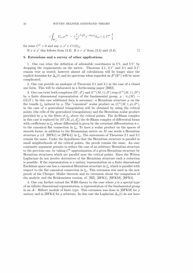
32 WITTEN HELFFER SJOSTRAND THEORY
|∫W−x′
Ux,teth − (
t
π)n−2q
4 e−th(x)δxx′ | ≤ C ′′1t
for some C ′′ > 0 and any x, x′ ∈ Cr(h)q.If x 6= x′ this follows from (3.3). If x = x′ from (3.3) and (3.4).
5. Extensions and a survey of other applications.
1. One can relax the definition of admissible coordinates in C1, and C1” bydropping the requirements on the metric. Theorems 2.1, 2.1” and 3.1 and 3.1”remain true as stated; however almost all calculations will be longer since theexplicit formulae for ∆q(t) and its spectrum when regarded on S∗(Rn) will be morecomplicated.
2. One can provide an analogue of Theorems 2.1 and 3.1 in the case of a closedone form. This will be elaborated in a forthcoming paper [BH2].
3. One can twist both complexes (Ω∗, d∗) and (C∗(M, τ), ∂∗) resp (C∗(M, τ), D∗)by a finite dimensional representation of the fundamental group, ρ : π1(M) →GL(V ). In this case additional data is necessary: a Hermitian structure µ on theflat bundle ξρ induced by ρ. The ”canonical” scalar product on (C∗(M, τ, ρ), ∂∗),in the case of a generalized triangulation will be obtained by using the criticalpoints (the cells of the generalized triangulation) and the Hermitian scalar productprovided by µ in the fibers of ξρ above the critical points. The de-Rham complexin this case is replaced by (Ω∗(M,ρ), d∗ρ) the de-Rham complex of differential formswith coefficients in ξρ whose differential is given by the covariant differentiation w.r.to the canonical flat connection in ξρ. To have a scalar product on the spaces ofsmooth forms, in addition to the Riemannian metric on M one needs a Hermitianstructure µ (cf. [BFK1] or [BFK4]) in ξρ. The statements of Theorems 2.1 and 3.1remain the same. Under the hypotheses that the Hermitian structure is parallel insmall neighborhoods of the critical points, the proofs remain the same. An easycontinuity argument permits to reduce the case of an arbitrary Hermitian structureto the previous one, by taking C0 approximation of a given Hermitian structure byHermitian structures which are parallel near the critical points. Since the WittenLaplacians do not involve derivatives of the Hermitian structure such a reductionis possible. If the representation is a unitary representation on a finite dimensionalEuclidean space one has a canonical Hermitian structure in ξρ which is parallel withrespect to the flat canonical connection in ξρ. This extension was used in the newproofs of the Cheeger- Muller theorem and its extension about the comparison ofthe analytic and the Reidemeister torsion, cf. [BZ], [BFK1], [BFKM], [BFK4].
4. One can further extend the WHS-theory to the case where ρ is a special typeof an infinite dimensional representation, a representation of the fundamental groupin an A− Hilbert module of finite type. This extension was done in [BFKM] for ρunitary and in [BFK4] for ρ arbitrary. In this case the Laplacian ∆q(t) do not have

D. BURGHELEA 33
discrete spectrum and it seems quite remarkable that Theorems 2.1 and 3.1 remaintrue. It is even more surprising that exactly the same arguments as presented abovecan be adapted to prove them. A particularly interesting situation is the case ofthe left regular representation of a countable group Γ on the Hilbert space L2(Γ)when regarded as an N (Γ) right Hilbert module of the von Neumann algebra N (Γ),cf.[BFKM] for definitions. One can prove that Farber extended L2−cohomology ofM, a compact smooth manifold with infinite fundamental group defined analytically(i.e. using differential forms and a Riemannian metric) and combinatorially (i.eusing a triangulation) are isomorphic and therefore the classical L2−Betti numbersand Novikov-Shubin invariants defined analytically and combinatorially are thesame. For this last fact see [BFKM] section 5.3.
The WHS-theory was a fundamental tool in the proof of the equality of theL2−analytic and the L2−Reidemeister torsion presented [BFKM].
5. One can further extend Theorems 1.1, 1,1’, 2.2, 2.2’, 3.3, 3.3’, to bordisms(M,∂−M,∂+M), and ρ a representation of Γ = π1(M) on an A−Hilbert moduleof finite type. In this case one has first to extend the concept of generalized trian-gulation to such bordisms. This will involve a pair (h, g) which in addition to therequirements C1-C3 is supposed to satisfy the following assumptions: g is productlike near ∂M = ∂−M ∪ ∂+M, the function h : M → [a, b] satisfies h−1(a) = ∂−M,h−1(b) = ∂+M, a, b regular values, and is linear on the geodesics normal to ∂Mnear ∂M. In case h is replaced by a closed 1-form the requirement is that thisform vanishes on ∂M. This extension was partly done in [BFK2] and was used toprove gluing formulae for analytic torsion and to extend the results of [BFKM] tomanifolds with boundary.
5. One can actually extend the WHS-theory to the case where h is a generalizedMorse function, i.e. the critical points are either nondegenerated or birth-death.This extension is much more subtle and very important. Beginning work in thisdirection was done by Hon Kit Wai in his OSU dissertation.
References
[AB] D.M.Austin, P.M.Braam, Morse Bott theory and equivariant cohomology, The Floermemorial volume, Progress in Math, Vol. 133 Birkhauser Verlag, 1995.
[BZ1] J. P. Bismut, W. Zhang, An extension of a theorem by Cheeger and Muller, Asterisque205 (1992), 1-209.
[BZ2] J. P. Bismut, W. Zhang, Milnor and Ray-Singer metrics on the equivariant determinant
of a flat vector bundle, GAFA 4 (1994), 136-212.
[B] D.Burghelea, WHS theory in the presence of symmetry (in preparation).

34 WITTEN HELFFER SJOSTRAND THEORY
[BH1] D.Burghelea, S. Haller, On the topology and analysis of closed one form I (Novikov’s
theory revisited), DG -0101043.
[BH2] D.Burghelea, S. Haller, On the topology and analysis of closed one form II (in prepara-tion).
[BFK1] D. Burghelea, L. Friedlander, T. Kappeler, Asymptotic expansion of the Witten defor-mation of the analytic torsion, J. of Funct. Anal. 137 (1996), 320-363.
[BFK2] D. Burghelea, L. Friedlander, T. Kappeler, Torsion for manifolds with boundary andgluing formulas, Math. Nacht. 208 (1999), 31-91.
[BFK3] D. Burghelea, L. Friedlander, T. Kappeler, Witten deformation of analytic torsion andthe Reidemeister torsion, Amer.Math.Soc.Transl.(2), 184 ,(1998), 23-39.
[BFK4] D. Burghelea, L. Friedlander, T. Kappeler, Relative torsion, Communications in Con-temporary Math., to appear in issue 1, 2001.
[BFK5] D. Burghelea, L. Friedlander, T. Kappeler, WHS-theory (book in preparation).
[BFKM] D. Burghelea, L. Friedlander, T. Kappeler, P. McDonald, Analytic and Reidemeister
torsion for representations in finite type Hilbert modules, GAFA, 6 (1996), 751-859.
[DR] G. De Rham, Varietes Differentiables, Hermann, Paris, 1980.
[F] A.Floer, Symplectic fixed points and holomorphic spheres, Comm.Math.Phys. 120 (1989)
575-671.
[HS1] B. Helffer, J. Sjostrand, Multiple wells in the semi-classical limit I, Comm PDE 9 (1984),
337-408.
[HS2] B. Helffer, J. Sjostrand, Puits multiples en mecanique semi-classique, IV Etude du com-
plexe de Witten, Comm PDE 10 (1985), 245-340.
[H] B. Helffer, Etude de Laplacien de Witten associe a une fonction de Morse degeneree,
Publications de l’Univ. de Nantes, 19...
[I] S. Illman, The Equivariant Triangulation Theorem for Actions of Compact Lie Groups,
Math. Ann. 262 (1983), 487-501.
[L] F. Laudenbach, On the Thom Smale complex (appendix in [BZ]), Asterisque, 205 (1992)
209-233.
[MS] D. McDuff, D.Salamon, Introduction to Symplectic topology, Calderon Press, Oxford,1995.

D. BURGHELEA 35
[M] K. H. Meier, G-Invariante Morse Funktionen, Manuscripta math. 63 (1989), 99-114.
[Po] M. Pozniak, Triangulation of smooth compact manifolds and Morse theory, Warwick
preprint 11 (1990).
[P] I. Prokhorenko, Morse Bott functions and the Witten Laplacian, Communications inAnalysis and Geometry, Vol 7, no 4 (1999), 841-918.
[Sm] S. Smale, On the gradient dynamical systems, Annals of Math. 74 (1961), 199-206.
[Wi] E. Witten, Supersymmetry and Morse theory, J. of Diff. Geom. 17 (1982), 661-692.
[V] A. Verona, Stratified Mapping-Structure and Triangulability, .LNM, v. 1102 (1984)
Springer- Verlag.

![THE LUND MONTE CARLO FOR JET FRAGMENTATION ......T SjOstrand/Lund Monte Carloforjet fragmentation 245 processes: e~e annihilation [10],leptoproduction or Regge phenomenology itis motivated](https://img.pdfslide.us/doc/110x75/60a033b8723cc37b475c4e1a/the-lund-monte-carlo-for-jet-fragmentation-t-sjostrandlund-monte-carloforjet.jpg)


![Abstract. arXiv:1202.1208v3 [math.AT] 8 Sep 2012 · arXiv:1202.1208v3 [math.AT] 8 Sep 2012 2 DAN BURGHELEA AND STEFAN HALLER set of Jordan cells and of the numbers ]Bc r+]Bo r 1:Here](https://img.pdfslide.us/doc/110x75/6053ba342cef7b1e9d02b7cf/abstract-arxiv12021208v3-mathat-8-sep-2012-arxiv12021208v3-mathat-8-sep.jpg)


![On Courant’s nodal domain property for linear ...helffer/Herrmannhelfferjourneelabo2017.pdf · refers to the PhD thesis of Horst Herrmann (Gottingen, 1932) [13]. Bernard Hel er,](https://img.pdfslide.us/doc/110x75/5b8832d67f8b9a1a248e7940/on-courants-nodal-domain-property-for-linear-helfferherrmannhe-refers.jpg)