A Shapley decomposition of carbon emissions without residuals

Energy Policy 30 (2002) 727–736

A Shapley decomposition of carbon emissions without residuals

Johan Albrechta,*, Delphine Fran-coisa, Koen Schoorsb

aFaculty of Economics and Business Administration Centre for Environmental Economics and Environmental Management (CEEM),

University of Ghent, Hoveniersberg 24, 9000 Ghent, BelgiumbUniversity of Oxford, SBS, 59, George Street, Oxford, OX1 2BE, UK

Abstract

Conventional decomposition techniques for historical evolutions of carbon emissions present path dependent factor weights of

selected variables next to significant residuals. Especially for analyses over long periods with many variables, high residuals make it

almost impossible to derive reliable conclusions. As an alternative, we present the Shapley decomposition technique for carbon

emissions over the period 1960–1996. This technique makes it possible to present a correct and symmetric decomposition without

residuals. The starting point of our analysis was an extended Kaya Identity with nine components.

In a study of four countries, the Shapley decomposition showed that the carbon intensity of energy use and the decarbonization of

economic growthFvariables that are targeted with current climate policy measuresFhave more effect on total emissions than

generally suggested in conventional decomposition exercises. Another interesting conclusion from our analysis was that the effect of

population growth on emissions can be for some countries more important than the decarbonization efforts. r 2002 Elsevier

Science Ltd. All rights reserved.

Keywords: Carbon dioxide emissions; (Shapley) decomposition; Kaya identity

1. Introduction

In many fields of social sciences, decompositiontechniques are used to help disentangle the impact ofvarious causal factors. An analysis of energy-relatedcarbon emission patterns and its driving factors canprovide essential information for policy studies onnational strategies and the use of flexible instrumentsin climate policy. A decomposition of total CO2

emissions over a number of contributing factors shedssome light on the importance of crucial parame-tersFlike the ongoing decarbonization of energyservices or the rate of autonomous energy efficiencyimprovementsFthat are used in scenarios to calculatethe possible cost of climate policy scenarios fordeveloped countries.While sophisticated forecast technologies are avail-

able for the latter type of exercises, traditional decom-position analyses with a limited number of factors stillyield important residuals, even over short periods oftime. Another problem is that the value of the

contribution assigned to any given factor depends onthe order in which the factors appear in the eliminationsequence. Factors that are not treated symmetrically leadto an important ‘path dependence’ problem (Shorrocks,1999). This strongly reduces the relevance of decomposi-tion exercises for studies over longer periods. Therefore,we present in this paper a Shapley decomposition ofcarbon emissions that eliminates both problems. Afteran introduction to the Kaya Identity, we first work withfour contributing factors or components (carbon/energy,energy/GDP, GDP/population and population) for theperiod 1960–1996. For the same data set, we present theShapley decomposition results next to the results from atraditional decomposition. Our calculations are based ondata for Belgium, France, Germany and the UnitedKingdom. In the next step, we decompose the first twofactors over three economic sectors (industry, transportand other sectors) and discuss the main findings fromthis detailed Shapley decomposition.

2. The Kaya identity and a decomposition for four

countries

The aim of a decompostion analysis is to reveal theimportance of distinct components or factors that drive

*Corresponding author. Tel.: +32-9-264-3474; fax: +32-9-264-

3599.

E-mail addresses: [email protected] (J. Albrecht), Delphi-

[email protected] (D. Fran-cois), [email protected] (K.

Schoors).

0301-4215/02/$ - see front matter r 2002 Elsevier Science Ltd. All rights reserved.

PII: S 0 3 0 1 - 4 2 1 5 ( 0 1 ) 0 0 1 3 1 - 8

historical data. The relative weight of each factor in theobserved change can be relevant information for policymeasures. In the field of climate policy, reliableinformation on the ongoing decarbonization of indus-trialized economies and on the sensitivity of energyintensity to energy price shocks is necessary input forpolicymakers. This information is necessary to evaluatevarious strategies to achieve the reduction targets of thesix Kyoto Protocol greenhouse gases, with or withoutinternational flexibility instruments.There are two broad categories of decomposition

techniques: input–output techniques and disaggregationtechniques. Both techniques have different data require-ments but the latter are more suitable for internationalcomparisons, which explains their widespread use. Formethodological details we refer to Liaskas et al. (2000)and Park (1992). A recent overview of methodologicalissues in cross-country/region decomposition techniquesis given by Zhang and Ang (2001). They apply twopopular conventional decomposition methods, i.e. theLaspeyres method and the arithmetic mean weightDivisia method, and two recently proposed perfectdecomposition methods, i.e. the refined Laspeyresmethod and the logarithmic mean weight Divisiamethod to two data sets and discuss the differences. Intheir definition, perfect methods give complete decom-position results regardless of the data pattern, asopposed to the conventional methods. To stimulatethe debate on the best decomposition method, wepresent in the next sections of this paper another perfectdecomposition method.Important residuals constitute the most serious

problem with conventional disaggregative decomposi-tion. Liaskas et al. (2000) decompose industrial CO2

emissions for a number of European countries. Theywork with two periods, 1973–1983 and 1983–1993, andthe factors in the decomposition are output, energyintensity, fuel mix and structure. For some countries, theweight of the residual in the decomposition over onlyten years exceeds the weight of three of the other fourcomponents. For the United Kingdom, the Netherlands,Italy, France, Finland, Spain, Denmark, Belgium andAustria, the weight of the structural componentFor thestructural economic effect on emissionsFis lower thanthat of the residual. Obviously, conclusions from thistype of analysis are not always straightforward. Forlonger periods and for analyses with more components,the residual becomes even more problematic. This isillustrated in the next section with data for Belgium,France, Germany and the United Kingdom. We firstpresent a mathematical expression of total emissions bymeans of the Kaya Identity (Kaya, 1990). This equationprovides a useful tool to decompose total nationalcarbon emissions (C):

C ¼ ðC=EÞðE=GDPÞðGDP=PÞP ð1Þ

The formula links energy-related carbon emissions(C) to energy (E), the level of economic activity(GDP=gross domestic product) and population (P).C=E denotes the carbon intensity of energy use, E=GDPis the energy intensity of economic activity and GDP=Pis the per capita income. At any moment in time, thelevel of energy-related carbon emissionsFnext toemissions that result from changes in land-useFcanbe seen as the product of the four Kaya Identitycomponents. For small to moderate changes in the Kayacomponents between any two years, the sum of thepercent changes in each of the variables closelyapproximates the percent change in carbon emissionsbetween those two years:

dðlnCÞ=dt ¼ dðlnC=EÞ=dtþ dðln E=GDPÞ=dt

þ dðlnGDP=PÞ=dtþ dðlnPÞ=dt: ð2Þ

The historical trends in the Kaya Identity componentsprovide a reference point for evaluating current andfuture climate policy projections of carbon emissions aswell as the key economic, demographic and energyintensity factors leading to those emissions. With theavailability of detailed data, the impact of for instancethe replacement of coal in electricity generation bynatural gas or nuclear power can be compared to theimpact of economic growth on energy-related emissions.The Kaya Identity can reveal interesting differencesbetween emission patterns of developed and developingcountries. For an analysis based on the Kaya Identity ofthe implications of emission trading under the KyotoProtocol for the US economy, we refer to Dougher(1999).

2.1. Kaya in the International Energy Outlook 2001

A global view is given in Table 1 with the KayaIdentity components for three world regions. A histor-ical analysis for the period 1970–1999 is complementedwith the reference case projections for 1999–2020 fromthe International Energy Outlook 2001 (EIA, 2001).Positive annual average growth rates of carbon emis-sions between 1970 and 1999 are found for developed aswell as for developing countries. For all countries,economic growth and population growth outpaceddeclines in energy intensity and carbon intensity ofenergy use. The average annual decline of carbonemissions of 5.4% in the 1990s in Eastern Europe andthe Former Soviet Union presents a special case. Thisdecline is the result of a severe drop in economic outputper capita (�4%/yr). The IEO2001 reference caseprojections illustrate that reductions of carbon emis-sions require accelerated declines in energy intensityand/or carbon intensity. Such changes may in turnrequire significant changes in the existing energyinfrastructure. It remains questionable whether thesenecessary changes can be realised in one or two decades.

J. Albrecht et al. / Energy Policy 30 (2002) 727–736728

Energy use in the transport sector will continue todepend on oil since there are currently few economicalalternatives. And if such an alternative would soonarrive (e.g. ethanol, bio-methanol, hydrogen, fuel celltechnology, etc.), reshaping the current fuel deliveryinfrastructure would take a long time.Furthermore, we need to consider actual political

decisions that will later have important consequences forenergy infrastructures and energy-related emissions.Several European countries already committed to acomplete phase-out of domestic nuclear power genera-tion. This decision will slow down the decline in carbonintensity as a result of the increased use of fossil fuels.

2.2. An analysis for four countries

In Table 2, we present for four European countriesdata for the period 1960–1996. Instead of working withaverage annual percentage changes as in Table 1, we stilluse the Kaya Identity but subdivide the total period inthree subperiods: the early years before the oil crisis(1960–1973), the oil crisis years (1974–1986) and recenthistory or the period after the oil crisis (1987–1996).Information on the used sources and calculations thatwere necessary to compile Table 2 are given in theappendix.Carbon or CO2 emissions did increase in the four

countries over the period 1960–1996 but the differencesare remarkable. Total emissions increased strongly inBelgium, Germany and France, but only modestly theUnited Kingdom (UK). It is important to note that the

different situation in the UK seems to be the result ofwhat happened in the early years of the analysis. From1960 to 1973, emissions in the UK did grow by only13.8% while emissions in Germany and France morethan doubled (+123% resp. +109%). Emissions inBelgium did increase by 85.1% from 1960 to 1973. Thesedivergent post-war evolutions depend on strategic (andeven environmental) fuel choices for electricity produc-tion and on the strong and uneven development ofenergy-intensive industries like iron and steel produc-tion, chemical manufacturing and mining. Londonexperienced a sequence of ‘killer smogs’ in the late1940s and early 1950s, leading to the Clean Air Act of1956 that imposed much lower sulfur dioxide concen-trations (Elsom, 1997). New technologies were installedand coal gradually was replaced by gas and oil. Theresult was a decline of carbon and sulfur dioxideemissions.A good example of the different evolution in energy-

intensive industries is the metals industry in the UK thatdid grow by only 0.06% per year during the period1954–1973. For that period the average annual growthrate of ‘all manufacturing’ was 0.88% with the highestgrowth rates found for instruments (+1.25%), electricalengineering (+1.39%) and vehicles (+1.38%). For theperiod 1973–1986, the metals industry faced an averageannual growth of �0.73% while the average for UKmanufacturing was �0.47% (Oulton and O’Mahony,1994). For countries like Belgium, the strong growth ofthe iron and steel industry was one of the drivingeconomic forces in the post-war era.

Table 1

Average annual percentage change in CO2 emissions and the Kaya Identity components by region, 1970–2020a

History Reference case projection

Parameter 1970–1980 1980–1990 1990–1999 1999–2010 2010–2020

Industrialized World

C/E (%) �0.5 �0.7 �0.5 0.0 0.1

E/GDP (%) �1.1 �2.0 �0.7 �1.3 �1.3GDP/P (%) 2.4 2.2 1.6 2.2 2.0

P (%) 0.9 0.7 0.6 0.5 0.4

C emissions (%) 1.7 0.2 1.0 1.4 1.1

Developing World

C=E (%) �0.8 �0.2 �0.7 �0.1 �0.1E=GDP (%) �0.4 0.9 �1.0 �1.4 �1.4GDP=P (%) 3.5 1.7 3.1 3.7 4.2

P (%) 2.2 2.1 1.7 1.7 0.8

C emissions (%) 4.6 4.5 3.1 3.9 3.5

Eastern Europe and the Former Soviet Union

C=E (%) �0.8 �0.3 �1.0 �0.2 �0.3E=GDP (%) 1.4 0.6 �0.5 �2.4 �2.6GDP=P (%) 2.4 0.6 �4.0 4.1 4.5

P (%) 0.9 0.7 0.0 0.0 0.0

C emissions (%) 3.9 1.6 �5.4 1.4 1.5

aSource: Energy Information Administration (2001).

J. Albrecht et al. / Energy Policy 30 (2002) 727–736 729

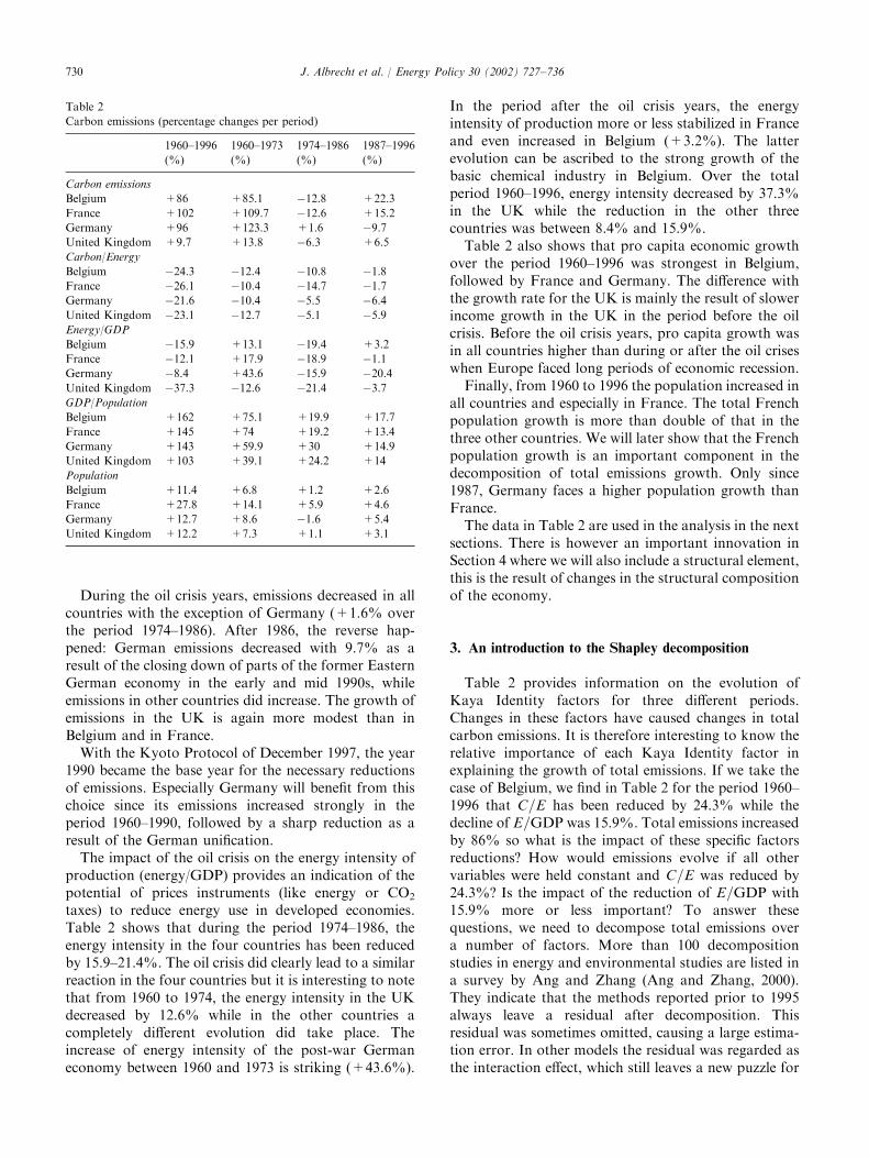
During the oil crisis years, emissions decreased in allcountries with the exception of Germany (+1.6% overthe period 1974–1986). After 1986, the reverse hap-pened: German emissions decreased with 9.7% as aresult of the closing down of parts of the former EasternGerman economy in the early and mid 1990s, whileemissions in other countries did increase. The growth ofemissions in the UK is again more modest than inBelgium and in France.With the Kyoto Protocol of December 1997, the year

1990 became the base year for the necessary reductionsof emissions. Especially Germany will benefit from thischoice since its emissions increased strongly in theperiod 1960–1990, followed by a sharp reduction as aresult of the German unification.The impact of the oil crisis on the energy intensity of

production (energy/GDP) provides an indication of thepotential of prices instruments (like energy or CO2

taxes) to reduce energy use in developed economies.Table 2 shows that during the period 1974–1986, theenergy intensity in the four countries has been reducedby 15.9–21.4%. The oil crisis did clearly lead to a similarreaction in the four countries but it is interesting to notethat from 1960 to 1974, the energy intensity in the UKdecreased by 12.6% while in the other countries acompletely different evolution did take place. Theincrease of energy intensity of the post-war Germaneconomy between 1960 and 1973 is striking (+43.6%).

In the period after the oil crisis years, the energyintensity of production more or less stabilized in Franceand even increased in Belgium (+3.2%). The latterevolution can be ascribed to the strong growth of thebasic chemical industry in Belgium. Over the totalperiod 1960–1996, energy intensity decreased by 37.3%in the UK while the reduction in the other threecountries was between 8.4% and 15.9%.Table 2 also shows that pro capita economic growth

over the period 1960–1996 was strongest in Belgium,followed by France and Germany. The difference withthe growth rate for the UK is mainly the result of slowerincome growth in the UK in the period before the oilcrisis. Before the oil crisis years, pro capita growth wasin all countries higher than during or after the oil criseswhen Europe faced long periods of economic recession.Finally, from 1960 to 1996 the population increased in

all countries and especially in France. The total Frenchpopulation growth is more than double of that in thethree other countries. We will later show that the Frenchpopulation growth is an important component in thedecomposition of total emissions growth. Only since1987, Germany faces a higher population growth thanFrance.The data in Table 2 are used in the analysis in the next

sections. There is however an important innovation inSection 4 where we will also include a structural element,this is the result of changes in the structural compositionof the economy.

3. An introduction to the Shapley decomposition

Table 2 provides information on the evolution ofKaya Identity factors for three different periods.Changes in these factors have caused changes in totalcarbon emissions. It is therefore interesting to know therelative importance of each Kaya Identity factor inexplaining the growth of total emissions. If we take thecase of Belgium, we find in Table 2 for the period 1960–1996 that C=E has been reduced by 24.3% while thedecline of E=GDP was 15.9%. Total emissions increasedby 86% so what is the impact of these specific factorsreductions? How would emissions evolve if all othervariables were held constant and C=E was reduced by24.3%? Is the impact of the reduction of E=GDP with15.9% more or less important? To answer thesequestions, we need to decompose total emissions overa number of factors. More than 100 decompositionstudies in energy and environmental studies are listed ina survey by Ang and Zhang (Ang and Zhang, 2000).They indicate that the methods reported prior to 1995always leave a residual after decomposition. Thisresidual was sometimes omitted, causing a large estima-tion error. In other models the residual was regarded asthe interaction effect, which still leaves a new puzzle for

Table 2

Carbon emissions (percentage changes per period)

1960–1996

(%)

1960–1973

(%)

1974–1986

(%)

1987–1996

(%)

Carbon emissions

Belgium +86 +85.1 �12.8 +22.3

France +102 +109.7 �12.6 +15.2

Germany +96 +123.3 +1.6 �9.7United Kingdom +9.7 +13.8 �6.3 +6.5

Carbon/Energy

Belgium �24.3 �12.4 �10.8 �1.8France �26.1 �10.4 �14.7 �1.7Germany �21.6 �10.4 �5.5 �6.4United Kingdom �23.1 �12.7 �5.1 �5.9Energy/GDP

Belgium �15.9 +13.1 �19.4 +3.2

France �12.1 +17.9 �18.9 �1.1Germany �8.4 +43.6 �15.9 �20.4United Kingdom �37.3 �12.6 �21.4 �3.7GDP/Population

Belgium +162 +75.1 +19.9 +17.7

France +145 +74 +19.2 +13.4

Germany +143 +59.9 +30 +14.9

United Kingdom +103 +39.1 +24.2 +14

Population

Belgium +11.4 +6.8 +1.2 +2.6

France +27.8 +14.1 +5.9 +4.6

Germany +12.7 +8.6 �1.6 +5.4

United Kingdom +12.2 +7.3 +1.1 +3.1


the reader (Sun, 1998). Some methods proposed after1995 are perfect, i.e. do not leave a residual term in theresults (Ang and Zhang, 2000). One of these perfectdecomposition methods is the one introduced by Sun(Sun, 1998). In his method, referred to as the refinedLaspeyres index method (Ang and Zhang, 2000), theinteractions (residual) are distributed equally among themain effects based on the ‘jointly created and equallydistributed’ principle. In order to do this, one has toassume that ‘there is no reason to assume contrary’.However, no further proof of the validity of thisassumption is given. Sun and Ang (2000) apply thesame principle to the Paasche and Marshall-Edgeworthforms. Contrary to the Laspeyres index model, whichadopts a prospective view, the Paasche index adopts aretrospective view. The Marshall-Edgeworth indexadopts a compromising view based on the Laspeyresand Paasche indices (Sun and Ang, 2000). The authorsprove that when the ‘jointly created and equallydistributed’ principle is applied to the Paasche andMarshall-Edgeworth models, the decomposition resultsare identical to the Laspeyres form results. But themethod implies the assumption made by Sun.Another perfect decomposition method discussed by

Ang and Zhang (2000) is the logarithmic mean Divisiamethod, proposed by Ang and Choi (1997). Theyreplaced the arithmetic mean weight function used inthe arithmetic mean Divisia index method by alogarithmic mean weight function. This refinementresults in a perfect decomposition, but one has to takeinto account the fact that using a logarithmic weightfunction implies the assumption of a constant growthrate. Furthermore, this refined Divisia method is basedon the normalization of the weight function, because thesum of the weight function over all sectors is not unity,but by definition always slightly less than unity (Angand Choi, 1997).We add to this literature by proposing a perfect

decomposition of carbon emissions based on theShapley value. Indeed, the decomposition problem hasformal similarities with a classical problem in co-operative game theory. Shapley (1953) was the first togive a formula for the real power of any given voter in acoalition voting game with transferable utility. This iscommonly referred to as the Shapley value. The Shapleyvalue is the mathematical expression of the real power ofa player when all orders of coalition formation areequiprobable. The Shaply value distributes the realpower among the players, satisfying three axioms,namely symmetry, no inessential players and additivity.Symmetry means that every player should be treatedsymmetrically in the estimation. No inessential playersmeans that players that do not contribute to the powerof any coalition do not receive any power. Additivitymeans that the power derived from every single possiblecoalition can be added to find the total real power.

Since 1953, the Shapley value has been used in anumber of cost allocation models. The properties ofsymmetry and no inessential players are very useful inthis context. A clear and simple explanation of how touse the Shapley value in cost allocation problems isgiven in Hamlen et al. (1977). Young et al.(1982)proposed to use the Shapley value to allocate costs inwater resources development projects. Kattuman et al.(1999) proposed to use the Shapley value to allocate thecosts of electricity transmission losses in the networkbetween several electricity generators. In these Shapley-value based cost allocation models everything happensas if the cost drivers enter the equation one by one, eachof them receiving their marginal contribution to thetotal cost. All orders of entering the cost equation areconsidered and receive the same weight 1=n! in thecomputation of the ultimate allocation of costs.Shorrocks (1999) points at the formal similarity

between the original Shapley value coalition problemand the general problem of allocating a certain amountof any output or cost among a set of agents, beneficiariesor cost drivers. Shorrocks builds on this similarity toconstruct a general decomposition procedure based onthe Shapley value (Shapley, 1953). Basically, thetechnique involves estimating the impact of eliminatingeach factor in succession, repeating this exercise for allpossible elimination sequences (the symmetry property)and then for each factor averaging its estimated impactover all the possible elimination sequences (the additiv-ity property). Let us consider what this concretelyimplies for the decomposition. In a simple ceteris paribustype decomposition one calculates the impact of eachvariable, leaving other variables constant. Because of theinteractions between several variables, this gives rise to aresidual. The literature has come up with several ways toavoid or allocate this residual (see higher). One simplemethod is to calculate the contribution of one variable,and then add cumulatively more and more variables.The result is a perfect decomposition without residuals.However, the order in which we include variables largelydetermines their calculated contribution because theallocation of the interaction effects depends on the orderof inclusion of the variable. Since the results depend onthe order by which variables enter the calculation, thiscumulative approach is path dependent and hencebiased. The underlying problem is that variables arenot treated symmetrically.The Shapley decomposition iterates the cumulative

approach for every possible order (permutation) ofvariables. With n variables, we need to make n!calculations, with each calculation based on anotherorder for including new variables. The Shapley valueimplies that taking the average of the n! estimatedcontributions for every variable, yields the true con-tribution of each variable. As a result, the Shapleydecomposition has three major advantages. First of all,


the decomposition is perfect, meaning that the sum ofthe impacts, allocated to each of the explanatoryvariables, equals the observed change in the decomposedvariable. One does not need to make any assumptions oreffort to allocate the residual, as the solution is free fromresiduals. Secondly, the Shapley decomposition issymmetric (or anonymous): the factors are treated inan even-handed manner, without making any furthertheoretical assumptions. Thirdly, the Shapley decom-position allows for very complex decompositions thatwould otherwise be troublesome because of very highresiduals and subsequent interpretation problems. Wewill illustrate the Shapley decomposition of a morecomplex identity in the next section.

4. Sectoral and structural effects in the decomposition

Starting from (1) and the data in Table 2, we addsectoral and structural effects to our analysis over theperiod 1960–1996. The change in carbon intensity ofenergy use and the change of energy intensity ofproduction can be due to changes within sectors (sectorsbecome more or less intensive in energy and carbon) orchanges between sectors (sectors that are intensive inenergy or carbon become more or less important in totalproduction). For simplicity, we work with three sectors:industry, transport and other sectors. For these threesectors, changes between 1960 and 1996 in the carbonintensity of energy and in the energy intensity of theproduction are calculated. For climate policy recom-

mendations, this type of information is essential,especially for analyses with extended time horizons. Byincluding these effects in our analysis, we have ninecomponents for the decomposition: three sectoralcarbon intensity effects (C=Eindustry; C=Etransport;C=Eother; denoted as Ci

j in (3)) three sectoral energyintensity effects (Ei in (3)), the effect of pro capita GDP(Ppc

o in (3)), the population effect (P in (3)) and thestructural effect. Name ajt the share of a sector j at time tin total production, the final equation for the change incarbon emissions over n sectors is presented in (3):

C ¼

Pnj¼1 ajtC

ijtE

ijt

� �Ppct Pt �

Pnj¼1 aj0C

ij0E

ij0

� �Ppc0 P0

Pnj¼1 aj0C

ij0E

ij0

� �Ppc0 P0

ð3Þ

As a result of the inclusion of sectoral and structuraleffects, there are some modest differences in the data,when comparing to the data used in Table 2. We explainour data in the appendix.We illustrate the problem of residuals in the basic

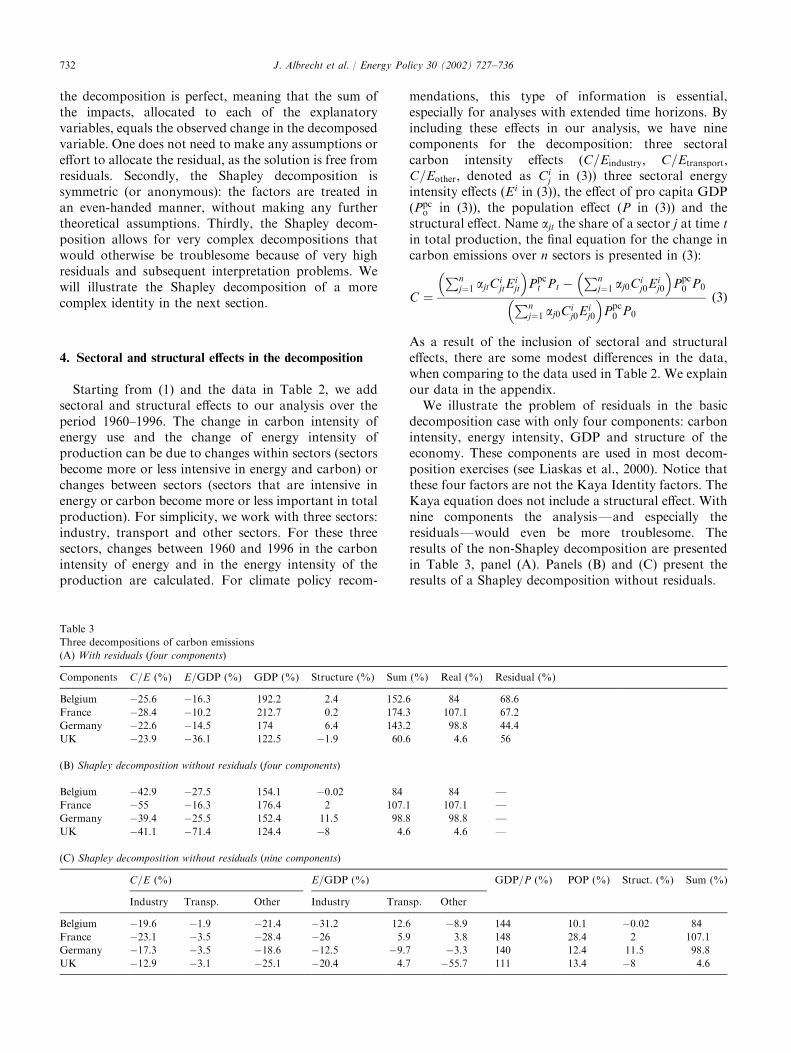
decomposition case with only four components: carbonintensity, energy intensity, GDP and structure of theeconomy. These components are used in most decom-position exercises (see Liaskas et al., 2000). Notice thatthese four factors are not the Kaya Identity factors. TheKaya equation does not include a structural effect. Withnine components the analysisFand especially theresidualsFwould even be more troublesome. Theresults of the non-Shapley decomposition are presentedin Table 3, panel (A). Panels (B) and (C) present theresults of a Shapley decomposition without residuals.

Table 3

Three decompositions of carbon emissions

(A) With residuals (four components)

Components C=E (%) E=GDP (%) GDP (%) Structure (%) Sum (%) Real (%) Residual (%)

Belgium �25.6 �16.3 192.2 2.4 152.6 84 68.6

France �28.4 �10.2 212.7 0.2 174.3 107.1 67.2

Germany �22.6 �14.5 174 6.4 143.2 98.8 44.4

UK �23.9 �36.1 122.5 �1.9 60.6 4.6 56

(B) Shapley decomposition without residuals (four components)

Belgium �42.9 �27.5 154.1 �0.02 84 84 FFrance �55 �16.3 176.4 2 107.1 107.1 FGermany �39.4 �25.5 152.4 11.5 98.8 98.8 FUK �41.1 �71.4 124.4 �8 4.6 4.6 F

(C) Shapley decomposition without residuals (nine components)

C=E (%) E=GDP (%) GDP=P (%) POP (%) Struct. (%) Sum (%)

Industry Transp. Other Industry Transp. Other

Belgium �19.6 �1.9 �21.4 �31.2 12.6 �8.9 144 10.1 �0.02 84

France �23.1 �3.5 �28.4 �26 5.9 3.8 148 28.4 2 107.1

Germany �17.3 �3.5 �18.6 �12.5 �9.7 �3.3 140 12.4 11.5 98.8

UK �12.9 �3.1 �25.1 �20.4 4.7 �55.7 111 13.4 �8 4.6


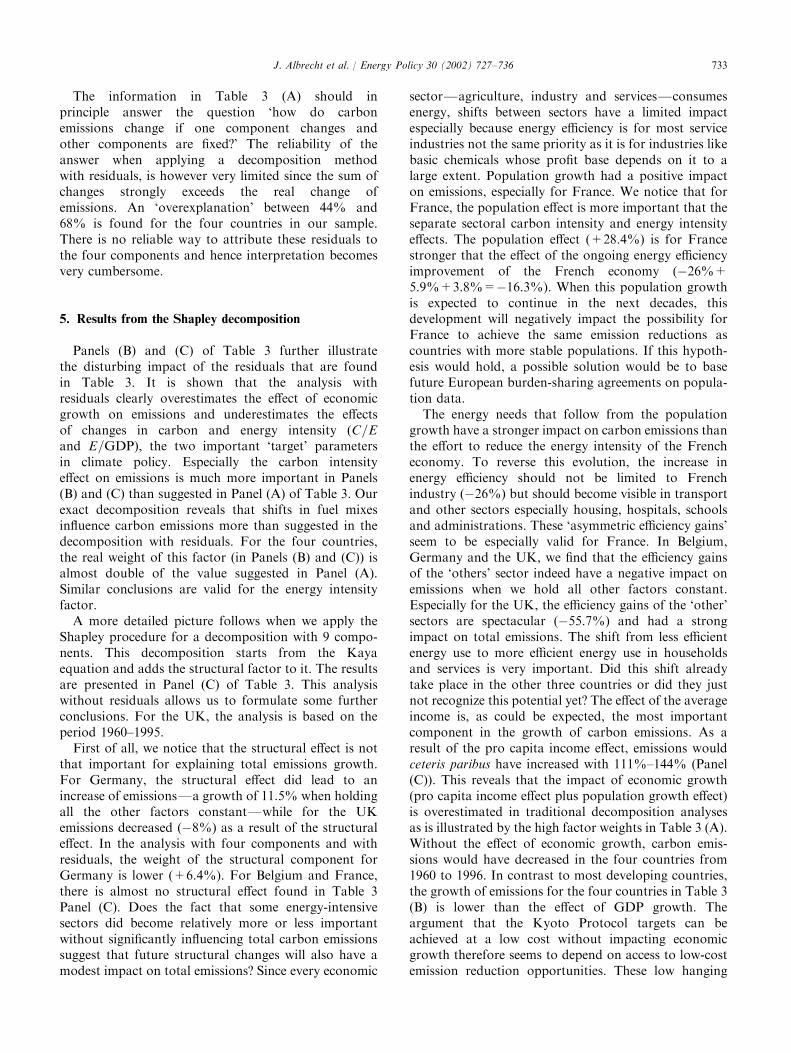
The information in Table 3 (A) should inprinciple answer the question ‘how do carbonemissions change if one component changes andother components are fixed?’ The reliability of theanswer when applying a decomposition methodwith residuals, is however very limited since the sum ofchanges strongly exceeds the real change ofemissions. An ‘overexplanation’ between 44% and68% is found for the four countries in our sample.There is no reliable way to attribute these residuals tothe four components and hence interpretation becomesvery cumbersome.

5. Results from the Shapley decomposition

Panels (B) and (C) of Table 3 further illustratethe disturbing impact of the residuals that are foundin Table 3. It is shown that the analysis withresiduals clearly overestimates the effect of economicgrowth on emissions and underestimates the effectsof changes in carbon and energy intensity (C=Eand E=GDP), the two important ‘target’ parametersin climate policy. Especially the carbon intensityeffect on emissions is much more important in Panels(B) and (C) than suggested in Panel (A) of Table 3. Ourexact decomposition reveals that shifts in fuel mixesinfluence carbon emissions more than suggested in thedecomposition with residuals. For the four countries,the real weight of this factor (in Panels (B) and (C)) isalmost double of the value suggested in Panel (A).Similar conclusions are valid for the energy intensityfactor.A more detailed picture follows when we apply the

Shapley procedure for a decomposition with 9 compo-nents. This decomposition starts from the Kayaequation and adds the structural factor to it. The resultsare presented in Panel (C) of Table 3. This analysiswithout residuals allows us to formulate some furtherconclusions. For the UK, the analysis is based on theperiod 1960–1995.First of all, we notice that the structural effect is not

that important for explaining total emissions growth.For Germany, the structural effect did lead to anincrease of emissionsFa growth of 11.5% when holdingall the other factors constantFwhile for the UKemissions decreased (�8%) as a result of the structuraleffect. In the analysis with four components and withresiduals, the weight of the structural component forGermany is lower (+6.4%). For Belgium and France,there is almost no structural effect found in Table 3Panel (C). Does the fact that some energy-intensivesectors did become relatively more or less importantwithout significantly influencing total carbon emissionssuggest that future structural changes will also have amodest impact on total emissions? Since every economic

sectorFagriculture, industry and servicesFconsumesenergy, shifts between sectors have a limited impactespecially because energy efficiency is for most serviceindustries not the same priority as it is for industries likebasic chemicals whose profit base depends on it to alarge extent. Population growth had a positive impacton emissions, especially for France. We notice that forFrance, the population effect is more important that theseparate sectoral carbon intensity and energy intensityeffects. The population effect (+28.4%) is for Francestronger that the effect of the ongoing energy efficiencyimprovement of the French economy (�26%+5.9%+3.8%=�16.3%). When this population growthis expected to continue in the next decades, thisdevelopment will negatively impact the possibility forFrance to achieve the same emission reductions ascountries with more stable populations. If this hypoth-esis would hold, a possible solution would be to basefuture European burden-sharing agreements on popula-tion data.The energy needs that follow from the population

growth have a stronger impact on carbon emissions thanthe effort to reduce the energy intensity of the Frencheconomy. To reverse this evolution, the increase inenergy efficiency should not be limited to Frenchindustry (�26%) but should become visible in transportand other sectors especially housing, hospitals, schoolsand administrations. These ‘asymmetric efficiency gains’seem to be especially valid for France. In Belgium,Germany and the UK, we find that the efficiency gainsof the ‘others’ sector indeed have a negative impact onemissions when we hold all other factors constant.Especially for the UK, the efficiency gains of the ‘other’sectors are spectacular (�55.7%) and had a strongimpact on total emissions. The shift from less efficientenergy use to more efficient energy use in householdsand services is very important. Did this shift alreadytake place in the other three countries or did they justnot recognize this potential yet? The effect of the averageincome is, as could be expected, the most importantcomponent in the growth of carbon emissions. As aresult of the pro capita income effect, emissions wouldceteris paribus have increased with 111%–144% (Panel(C)). This reveals that the impact of economic growth(pro capita income effect plus population growth effect)is overestimated in traditional decomposition analysesas is illustrated by the high factor weights in Table 3 (A).Without the effect of economic growth, carbon emis-sions would have decreased in the four countries from1960 to 1996. In contrast to most developing countries,the growth of emissions for the four countries in Table 3(B) is lower than the effect of GDP growth. Theargument that the Kyoto Protocol targets can beachieved at a low cost without impacting economicgrowth therefore seems to depend on access to low-costemission reduction opportunities. These low hanging


fruits can probably be found in developing or transi-tional countries.Table 3 (C) shows that for industry, the decrease in

energy intensity had an important impact on totalemissions for all countries. This effect is strongestfor Belgium where the increasing energy efficiency ofindustry could reduce emissions by 31.2% whenother factors are held constant. For Germany, thiseffect is weakest (�12.5%). There is still no indicationof a trend towards increased energy efficiency inthe transport sector. Cleaner and more fuel-efficienttransport equipment can not compensate the stronggrowth of transport activities in most developedcountries. Another explanation can be the decliningmarket share of rail transport in the container market incountries like Belgium. Holding all other componentsconstant, the evolution of the transport energy intensitywould lead to increasing emissions in Belgium, Franceand the UK.Only for Germany, the impact would be negative.

With respect to the carbon intensity of energy use, thereare only minor differences between the four countries.The impact of the change in industrial carbon intensityon total emissions is between �12.9% (UK) and�23.1% (France). The impact of carbon intensitychanges in transport is very similar: between �1.9%for Belgium and �3.5% for France and Germany. Thisis not a surprise since transport infrastructure is verysimilar in the four countries. The impact of other carbonintensity changes is more diverging. For Germany, wefind the lowest value with �18.6%. For France thiseffect is most important: �28.4%.

6. Growth versus component weight

When we compare Table 2 to Table 3 (B) and (C),some points deserve our further attention. For the fourcountries, the differences in the carbon intensity ofenergy use during the period 1960–1996 seem to bemodest in Table 2. Table 3 (B) shows that similarevolutions in carbon intensity (from �21.6% forGermany to �26.1% for France, see Table 2) can havea different impact on total emissions (from �39.4% to�55%). Precisely this impact provides the most usefulinformation for further policy development. The differ-ence in carbon intensity between France and Belgium isonly 1.8% (see Table 2) while the difference in totalweight is 12.1% (see Table 3 (B)). Holding all othercomponents constant, similar reductions in carbonintensity can lead to different reductions in carbonemissions because of structural differences betweendifferent economies. We therefore need to be aware ofall the interaction effects that take place inside theeconomy. The evolution of one single variable can beinteresting but the impact of this single variable on total

emissions depends on the evolution of other variablesas well. The more interactions are included in theanalysis, the more reliable the reported effects will be.This explains why we opted for an extended Kayaequation with nine components. Of course, we do notclaim that this extended equation captures all relevantinteractions.The differences in the evolution of the energy intensity

of production also correspond to more explicit differ-ences in the weight of this factor in the decomposition.The difference between Belgium and France is 3.8% (seeTable 2: �15.9% versus �12.1%) while the difference inthe total weight of this factor is 11.2% (�27.5% versus�16.3% in Table 3 (B)). Similarly, compared to the UK,E=GDP is 25.2% lower in France (�37.3% versus�12.1%). The total weight of this factor is for the UK�71.4% while it is only �16.3% for France.These findings illustrate again that similar trends for

parameters in Table 2 can be the result of very differentevolutions in similar developed economies and viceversa.

7. Conclusions

Starting from the Kaya Identity, we presented aShapley decomposition for carbon emissions forfour European countries. This technique makes itpossible to present a perfect and symmetric decomposi-tion without residuals. Compared to conventionaldecomposition techniquesFwith residuals that amountto more than 50% of carbon emission growthFthis is apromising improvement offering valid and reliableinformation on complex questions such as the impor-tance of specific energy-related evolutions in totalemissions growth.From a limited analysis for four countries, we found

that the Shapley decomposition showed that factorslike the carbon intensity of energy use and thedecarbonization of economic growth have moreeffect on total emissions than suggested in conventionaldecomposition exercises. In these exercises, the effectof economic growth on emissions is overestimatedfor developed countries since this important variablecaptures a significant part of the residuals. But thereal weight of this variable is lower and the weight ofthe other variablesFthose that are the essence ofclimate policyFis higher. These results seem tosuggest that fuel mix changes and the ongoing decarbo-nization can in interaction with other effects play animportant role in climate policy. Another interestingconclusion from our analysis was that the effect ofpopulation growth on emissions can be for somecountries be more important than the decarbonizationefforts.


Appendix A

Population

Source: OECD Energy Balances.

GDP

global Kaya IdentitySource: OECD National Accounts, I. We used the

Gross Domestic Product (Expenditure) data in US $ atexchange rates and price levels of 1990.

sectoral decompositionSource: OECD National Accounts, II, Value Added

by Kind of Activity approach (for compatibility reasonswith the decomposition of the Energy data).

Sectoral decomposition calculations for each separatecountry were as follows:

Belgium (MN FB90 Price); France (MN FF80 Price)

Total Industry Sector GDP=Manufacturing+Elec-tricity, Gas and Water+ConstructionTotal Transport Sector GDP=Transport and StorageTotal Other Sectors GDP=Gross Domestic Pro-

duct�Total Industry Sector GDP�Total TransportSector GDP

Germany (MN DM 91 Price)

German ‘Value Added’ GDP data were only availablefrom 1991. For the years 1960–1990 we used data fromthe former Federal Republic of Germany and added10% as this was estimated to be the GDP share of theformer German Democratic Republic. We assumed thatthe different sectors were equally represented in bothparts of the country, knowing that this would lead toonly minor distortions of the data.

Germany 1991–1996

Total Industry Sector GDP=Manufacturing+Con-structionTotal Transport Sector GDP=Transport, Storage

and CommunicationTotal Other Sectors GDP=Gross Domestic Pro-

duct�Total Industry Sector GDP�TotalTransport Sector GDP

Germany 1960–1990

Total Industry Sector GDP=Manufacturing+Elec-tricity, Gas and Water+ConstructionTotal Transport Sector GDP=Transport and StorageTotal Other Sectors GDP=Gross Domestic Pro-

duct�Total Industry Sector GDP�Total

Transport Sector GDP

United Kingdom (MN PS Curr. Price)

Total Industry Sector GDP=Manufacturing+Elec-tricity, Gas and Water+ConstructionTotal Transport Sector GDP=Transport, Storage

and CommunicationTotal Other Sectors GDP=Gross Domestic Pro-

duct�Total Industry Sector GDP�TotalTransport Sector GDP

The baseyear and the used currencies differ fromthose used in the global Kaya Identity. We thereforemultiplied all sectoral GDP data by correction factors(GDP used in global Kaya formula/‘Value Added’GDP) for each year.

EnergySource: OECD Energy Balances.We opted for Total Final Consumption as a basic

concept in calculating the Carbon and Energy KayaIdentity Factor. Total Final Consumption is the sum ofconsumption by the different end-use sectors. The reasonfor this choice is the fact that Total Final Consumptiondata can easily be disaggregated into different sectors,more specifically the industry sector, the transport sectorand the other sectors (Agriculture, Commerce and Publ.Serv., Residential and Non-specified). We did notinclude Non-Energy Use. A correction factor wasincluded when comparing the sum of the sectoraldecompositions with the global Kaya results.

CarbonTotal Final Consumption data comprise the use of

different energy sources, as well as Electricity and Heat.The decomposition of Electricity and Heat is based ondata from Electricity Plants, CHP Plants and HeatPlants. Emission factors from fossil fuel combustionwere found in the ‘Second Netherlands’ NationalCommunication on Climate Change Policies’ and the‘Revised 1996 IPPC Guidelines for National Green-house Gas Inventories: Reference Manual’.

References

Ang, B.W., Choi, K.H., 1997. Decomposition of aggregate energy and

gas emission intensities for industry: a refined Divisia index

method. The Energy Journal 18 (3), 59–73.

Ang, B.W., Zhang, F.Q., 2000. A survey of index decomposition

analysis in energy and environmental studies. Energy 25,

1149–1176.

Dougher, R., 1999. The Kyoto Protocol: implications of emissions

trading scenarios. American Petroleum Institute Research Paper

#095, July.


Elsom, D., 1997. Atmospheric pollution trends in the United

Kingdom. In: Simon, J. (Ed.), The State of Humanity. Blackwell,

Oxford, UK.

Energy Information Administration, 2001. International Energy

Outlook 2001. Washington DC, March 28.

Hamlen, S.S., Hamlen, W.A., Tschirhart, J.T., 1977. The use of core

theory in evaluating joint cost allocation schemes. Accounting

Review 52 (3), 616–0627.

Kattuman, P.A., Bialek, J.W., Abi-Samra, N., 1999. Electricity

Trading and Co-operative Game Theory. Proceedings of the 13th

Power System Computation Conference, Trondheim, June 28–July

2, 1999, pp. 238–243.

Kaya, Y., 1990. Impact of carbon dioxide emission control on GNP

growth: interpretation of proposed scenarios. Paper presented at

the IPCC Energy and Industry Subgroup, Response Strategies

Working Group, Paris, France.

Liaskas, K., Mavrotas, G., Mandaraka, M., Diakoulaki, D., 2000.

Decomposition of industrial CO2 emissions: the case of European

union. Energy Economics 22, 383–394.

Oulton, N., O’Mahony, M., 1994. Productivity and Growth. A study

of British Industry, 1954–1986. Cambridge University Press,

Cambridge.

Park, S.-H., 1992. Decomposition of industrial energy consumption:

an alternative method. Energy Economics 14, 265–270.

Shapley, L., 1953. A value for n-person games. In: Kuhn, H.W.,

Tucker, A.W. (Eds.), Contributions to the theory of games, Vol. 2.

Princeton University, Princeton, NJ.

Shorrocks, A.F., 1999. Decomposition procedures for distributional

analysis: a unified framework based on the Shapley value. Mimeo,

University of Essex.

Sun, J.W., 1998. Changes in energy consumption and energy

intensity: a complete decomposition model. Energy Economics

20, 85–100.

Sun, J.W., Ang, B.W., 2000. Some properties of an exact energy

decomposition model. Energy 25, 1177–1188.

Young, H.P., Okada, N., Hashimoto, T., 1982. Cost allocation in

water resources development. Water Resources Research 18 (3),

463–475.

Zhang, F.Q., Ang, B.W., 2001. Methodological issues in cross-

country/region decomposition of energy and environment indica-

tors. Energy Economics 23, 190–197.


Documents

A Shapley decomposition of carbon emissions without residuals