A shallow geothermal experiment in a sandy aquifermonitored using electric resistivity tomography

Thomas Hermans1, Alexander Vandenbohede2, Luc Lebbe2, and Frédéric Nguyen3

ABSTRACT

Groundwater resources are increasingly used around theworld for geothermal exploitation systems. To monitor suchsystems and to estimate their governing parameters, we relymainly on borehole observations of the temperature field at afew locations. Bulk electric resistivity variations can bringimportant information on temperature changes in aquifers.We have used surface electric resistivity tomography to monitorspatially temperature variations in a sandy aquifer during a ther-mal injection test. Heated water (48°C) was injected for 70 hoursat the rate of 87 l∕h in a 10.5°C aquifer. Temperature changesderived from time-lapse electric images were in agreement withlaboratory water electric conductivity-temperature measure-ments. In parallel, a coupled hydrogeologic saturated flow

and heat transport model was calibrated on geophysical data forthe conceptual model, and on hydrogeologic and temperaturedata for the parameters. The resistivity images showed an upperflow of heated water along the well above the injection screensand led to a new conceptualization of the hydrogeologic sourceterm. The comparison between the temperature models derivedfrom resistivity images and from the simulations was satisfac-tory. Quantitatively, resistivity changes allowed estimating tem-perature changes within the aquifer, and qualitatively, the heatedplume evolution was successfully monitored. This work demon-strates the ability of electric resistivity tomography to study heatand storage experiments in shallow aquifers. These results couldpotentially lead to a number of practical applications, such as themonitoring or the design of shallow geothermal systems.

INTRODUCTION

Groundwater plays a major part in the production of geothermalenergy, which is increasingly growing worldwide. For instance, in2010, geothermal heat pumps accounted for 47.2% of thermal en-ergy use and 68.3% of total installed capacity in the world (Lund,2010). Geothermal energy resources therefore constitute an essen-tial field of research and development in the diversification ofenergy resources to hinder global warming.Very-low temperature systems (<30°C) are much more easily ac-

cessible and involve lower implementation costs than deeper hightemperature systems. Moreover, very-low temperature systems,such as shallow aquifers, are relatively abundant in alluvial or coast-al plains where urban development concentrates. From 0 to less than100 meters depth, groundwater has an average temperature ranging

from 5°C to 30°C and may be used for cooling or heating (Allen andMilenic, 2003).Exploitation of geothermal energy relies on either extraction (or

storage) of groundwater (or heated water) through pumping (orinjection) wells or on heat exchange between the geological med-ium and a fluid circulating in a closed and buried circuit (Lund et al.,2005). To design such systems, engineers must estimate the param-eters governing heat transport processes, which are mainly heatcapacity and thermal conductivity of fluid and solid (Busby et al.,2009). Engineers generally rely on standard calculation charts,which may not be representative of in situ conditions, such asthe influence of the soil/rock, the well and the fluid, or onthermal response tests in wells, which deliver only well-centeredinformation (similar to pumping tests). In this context, electric re-sistivity tomography (ERT) can bring relevant spatial and temporal

Manuscript received by the Editor 9 June 2011; revised manuscript received 8 September 2011; published online 13 February 2012.1University of Liege, Department ArGEnCo, Applied Geophysics, Liege, Belgium and F.R.S.-FNRS, Aspirant, Brussels, Belgium. E-mail: thomas.hermans@

ulg.ac.be.2Ghent University, Department of Geology and Soil Science, Research Unit Groundwater Modelling, Ghent, Belgium. E-mail: alexander.vandenbohede@

ugent.be; luc.lebbe@ugent.be.3University of Liege, Department ArGEnCo, Applied Geophysics, Liege, Belgium. E-mail: f.nguyen@ulg.ac.be.

© 2012 Society of Exploration Geophysicists. All rights reserved.

B11

GEOPHYSICS, VOL. 77, NO. 1 (JANUARY-FEBRUARY 2012); P. B11–B21, 9 FIGS., 1 TABLE.10.1190/GEO2011-0199.1

Downloaded 15 Feb 2012 to 139.165.125.85. Redistribution subject to SEG license or copyright; see Terms of Use at http://segdl.org/

information through the correlation between temperature and bulkelectric resistivity changes with a greater coverage than single wellsfor in situ studies.Bulk electric resistivity of soil/rock samples decreases with

temperature (e.g., Revil et al., 1998; Hayley et al., 2007). Thiscorrelation reflects the change in conductivity of water containedin the pores but also in the surface conductivity of grains. The firsteffect is related to changes in the fluid viscosity, whereas the secondis due to changes in the surface ionic mobility. As a result, tempera-ture corrections in time-lapse series may be necessary to correctelectric resistivity tomography results to avoid misinterpretationwhen explaining resistivity changes (e.g., Hayley et al., 2007,2010; Ma et al., 2011).Geothermal experiments have been performed for several

decades in hydrogeology. Buscheck et al. (1983), Molson et al.(1992), or Vandenbohede et al. (2009), for example, simulate ther-mal injection and recovery experiments and heat tracing (e.g.,Anderson et al., 2005, for a review) tests have been used to studygroundwater reservoirs.A parallel can be done between temperature monitoring

(Anderson, 2005) and salt tracer test (Ptak et al., 2004). Tempera-ture and salt concentration both have an effect on fluid and surfaceelectric conductivity (Revil et al., 1998). As shown recently bySingha et al. (2011), traditional chemically conservative tracersmay not be electrically conservative due to phenomena like ion ex-changes, mass transfers, or surface conductance. Temperature mayalso modify chemical processes by changing equilibrium constantsor reaction kinetics. Both effects modify the density of the fluid, butin an opposite way. Saline tracers can be used to generate very highelectrical resistivity contrasts (typically around 10 to 1), but an in-crease in salinity will increase water density and potentially lead thetracer to sink down the aquifer (e.g., Kemna et al., 2002). It is dif-ficult to reach such a contrast with heat tracers, but an increase intemperature will decrease the density, which is favorable whenmonitoring from the surface because the injected tracer will notsink. An analogy exists concerning the flow and transport modelfor both types of tracer (e.g., Anderson, 2005; Langevin et al.,2010), but using thermal tracers enables the derivation of governingparameters for heat transport processes. The monitoring design withERT will be similar for both cases, but the interpretation needs touse appropriate petrophysical relationships.ERT has been applied to study heat reservoirs where hydrother-

mal fluids generate high resistivity contrasts due to their tempera-ture often exceeding 150°C. In those situations, ERT can detect thereservoir itself, map preferential flow paths, and is useful to char-acterize rock properties (e.g., Pérez-Flores and Gomez Trevino,1997; Bruno et al., 2000; Garg et al., 2007; Arango-Galván et al.,2011). Recently, several studies were carried out to image volcanohydrothermal systems with very long resistivity cables, showingthat ERT is a reliable tool to detect hydrothermal features (e.g.,Revil et al., 2010, 2011). ERT has also been used to study seasonalchanges in permafrost rock walls. A resistivity-temperature rela-tionship was calibrated around and below the freezing point to givequantitative information on frozen rock temperatures (Krautblatteret al., 2010).Time-lapse measurements were also used to monitor geothermal

systems. Legaz et al. (2009) used ERT and self-potential measure-ments to image the effect of the variations in Inferno Crater Lake

level in New Zealand. ERT highlighted a large decrease in resistiv-ity as the water level in the lake decreased.Ramirez et al. (1993) use cross-borehole time-lapse ERT to moni-

tor a steam injection during a restoration process. Changes in resis-tivity were related to an increase in water and soil temperature, adisplacement of pore water and changes in ionic content ofthis water.LaBrecque et al. (1996b) monitored temperature changes in the

context of Joule heating combined to vapor extraction during aremediation process with cross-boreholes time-lapse ERT. Theycompared their results with temperature measurements but didnot proceed to a conversion of ERT results into temperature. Theyanalyzed differences in conductivity cell by cell to remove the spa-tial variability influence which remains constant during the heating.After 7 days of heating, the mean temperature increased by 17°C,they found mean temperatures in agreement with their expectations.After 14 days, the temperature reached 100°C and the change inconductivity was bigger than expected by temperature effects only.It was explained by a decrease in saturation. After 28 days ofheating, conductivites were much below the background valuesshowing an important loss of water produced by desaturation.To our knowledge, few studies have used time-lapse surface ERT

to estimate the characteristics of heat exchange and fluid transportduring a geothermal tracer experiment at low temperature and smallscale, typical of very-low enthalpy geothermal systems. Benderitterand Tabbagh (1982) carried out an experiment where injectedheated water in a 4 to 7 m depth confined aquifer was monitoredwith DC resistivity measurements. The electric current wasinjected into two electrodes and the potential was measured at amoving electrode with reference to a fixed one. The authors pro-duced qualitative anomaly maps using percentage changes in poten-tial. Due to limited computing power, these maps were interpretedusing electric forward modeling of resistivity anomalies calculatedfor simple geometric subsurface models determined according tothe injected volume. The existence of an electric anomaly in bulkelectric resistivity (−33%) resulting from injection of heated water(40°C) was clearly demonstrated.In this paper, we examine the potential of ERT to image an in-

jection and storage experiment using heated water, and its contribu-tion in calibrating coupled flow and heat transport models. Theheated plume evolution was successfully imaged by ERT as itwas injected in one well. Combined with temperature well logs,ERT images contributed to detect leakage in the injection welland to calibrate the source term in the thermohydrogeologicmodel. In addition, ERT-derived temperatures in the aquifer seemin accordance with the latter model.The paper is organized as follows. First the study site is pre-

sented. Then, the methodology of the experiment is described:the injection procedure, petrophysical relationships, the thermo-hydrogeologic model, error assessment, and the inversion methodare presented. The results section describes the background study ofthe site and the comparison to borehole data to validate ERT images.Results of time-lapse data collected after injection are also pre-sented and are compared to thermohydrogeologic modeling results.

FIELD SITE

The field experiments took place on the campus De Sterre ofGhent University, Belgium, from 8 to 12 February 2010 (Figure 1).Figure 2 shows a schematic cross section of the site with lithological

B12 Hermans et al.

Downloaded 15 Feb 2012 to 139.165.125.85. Redistribution subject to SEG license or copyright; see Terms of Use at http://segdl.org/

characteristics and the position of the water level, together with thewell description. The upper layer lies from 0 to −2 m andcorresponds to unsaturated fine sands. From −2 m down to−4.4 m, the same sands are found at saturation. These sands con-stitute homogeneous Quaternary deposits, as evidenced by nearbyboreholes (W02 and W03 on Figure 1). Below −4.4 m, a clay layerof Tertiary age is found, forming a low permeability layer. The in-jecting well was drilled down to −4.4 m, it is made of a PVC casingwith a screen of 90 cm at the bottom of the Quaternary layer.Calibrated sands were poured around the well along the screen,and bentonite cement was used to fill the upper part of the drillinghole as a hydraulic seal. The water table lies at −2 m and is nearlyflat on the site; a gradient of 0.005 toward thesouth-southwest was derived from three wells(W01, W02, and W03 on Figure 1). The tem-perature in the aquifer was 10.5°C.

METHODS

Heating and injection of water

A slug test was performed in the injection wellto estimate possible injection rates. A volume of10 l was injected and the evolution of the hydrau-lic head was followed with a pressure transducer.For a water temperature of 10.5°C, a maximumrate of 70 l∕h was estimated. However, for waterat 48°C, the decrease in viscosity enabled an in-jection rate of 87 l∕h.For practical reasons, it was not possible to

heat the formation water directly. This wouldhave required two new pumping wells and wouldhave led to logistics problems: control of pump-ing rates during all the experiment and storage ofpumped formation water in containers outside ofthe building in cold air conditions before heating.Access to the unconfined aquifer was only pos-sible in the injection well. Other wells intersect-ing the unconfined aquifer were located on the other side of the road(Figure 1). The use of resistance to heat the water through Jouledissipation (LaBrecque et al., 1996b) was not considered becauseit would only lead to conduction and no convection.Tap water was thus used for the injection. Its temperature fluc-

tuated between 9°C and 14°C. After passing through a heating sys-tem consisting of two electric boilers having a capacity of 200 l anda power of 2200 W, water temperatures varied between 45°C and49°C, with an average of 48°C. Injection of heated water started at 9February and lasted for 70 hours.

Petrophysical relationships

In this section, we will describe the relationship between tem-perature and water electric conductivity as well as the one betweenwater electric conductivity and bulk electric conductivity.A linear dependence between electric conductivity and tempera-

ture of soil/rock can be assumed when limited temperature intervalsare considered (a few tens of degrees). Equation 1 expresses thelinear relation around 25°C (Hayley et al., 2007):

σTσ25

¼ mðT − 25Þ þ 1; (1)

where σT is the electric conductivity of soil/rock at temperature T(in °C), m is the fractional change in electric conductivity perdegree Celsius. The value of m can be experimentally determinedand varies according to the type of fluid and sediments. A valuebetween 0.018 °C−1 and 0.025 °C−1 is often found for m (Hayleyet al., 2007). Water and surfaces conductivity effects may beseparated and expressed by similar equations with different frac-tional changes, mf and ms, respectively. Revil et al. (1998) foundmf equal to 0.023°C−1 and ms around 0.04°C−1 for surfaceconductivity on the temperature range 25°C–200°C. The ratio ofsurface conductivity to the fluid conductivity increases withtemperature and equation 1 does not apply for bulk conductivity.

Figure 1. The study area is located on the campus De Sterre of Ghent University; W01gives the position of the injection well, W02 and W03 the position of two wells used todescribed the water level. The black line shows the position of ERT profile next to thegeological institute.

water level

fine sand

sandy clay

0

– 2

– 4.4

– 12

Dep

th (

m)

Figure 2. The first 4.4 meters of the field site consist of fine sands.These sands cover a sandy clay layer which is less permeable. Thewater level lies at −2 m. The injection well is drilled in the finesands and is screened between −3.5 and −4.4 m.

Shallow geothermal test monitored with ERT B13

Downloaded 15 Feb 2012 to 139.165.125.85. Redistribution subject to SEG license or copyright; see Terms of Use at http://segdl.org/

Hayley et al. (2007) apply the same model as Revil et al. (1998) onthe temperature range 0°C–25°C and found ms around 0.018 °C−1

and mf equal to 0.0187 (Hayashi, 2004). These values are similar,leading globally to linear temperature dependence for the bulk elec-tric resistivity.Archie’s law (equation 2) describes the link between the forma-

tion factor F and the porosity ϕ through the cementation exponentm (Archie, 1942):

1

F¼ ϕm: (2)

The formation factor is used to link the bulk and fluid electricconductivity (equation 3) when surface conductivity can beneglected:

σb ¼σfF; (3)

where σb is the bulk electric conductivity of the soil/rock in S∕mand σf is the electric conductivity of the fluid in S∕m. Equation 3does not involve surface conductivity. When the matrix conductiv-ity is nonnegligible, in shaly and clayey sediments for example,additional terms are needed to take into account the surface conduc-tivity of the solid. Equation 4 generalizes equation 3 to include thesurface conductivity σs:

σb ¼σfF

þ σs: (4)

Several authors (e.g., Waxman and Smits, 1968; Revil et al.1998) give more complex equations to take into account the surfaceconductivity, using, for example, the cation exchange capacity.In saturated sediments, equation 3 shows that the bulk electric

conductivity is directly proportional to the fluid electric conductiv-ity if we neglect the surface conductivity. In our study, theexperiment took place in sandy sediments free of clays from thesurface down to −4.4 m. Several authors (e.g., Revil et al.,1999; Revil and Linde, 2006; Bolève et al., 2007; Leroy et al.,2008) showed that silica grains have a surface conductivity, whichcannot be neglected if the water is fresh enough (e.g., Jardani et al.,

2009). According to Revil and Linde (2006), the surface electricconductivity increases when the diameter of the particles decreases:

σs ¼6Σs

d0; (5)

where Σs is the specific surface conductivity in siemens and d0 isthe mean particle diameter in meters. If we assume the specific sur-face conductivity given by Bolève et al. (2007), 4.0 × 10−9 S and amean particle size diameter for the fine sands of 200 μm, we found asurface conductivity of 1.2 × 10−4 S∕m, which is three orders ofmagnitude below the water electric conductivity on the site, i.e.,around 0.1 S∕m. The role of the sediment surface electric conduc-tivity was thus neglected.In the clays of Tertiary age, equation 4 should be used to take into

account the change in surface conductivity. Interpretation in termsof temperature was not considered in the clays because the surfaceconductivity effect cannot be neglected. Clay acts as an imperme-able barrier avoiding convection processes, but conduction is stillpossible, leading to an increase in temperature of the clay.In the unsaturated zone, Archie’s law (equation 3) can be ex-

tended to account for water saturation Sw

σb ¼σfF

Snw; (6)

where n is an empirical exponent close to two. In consequence,electric conductivity changes in the unsaturated zone may be relatedto either saturation or temperature changes.In the 10°C–50°C temperature interval considered for this experi-

ment, a linear relationship can describe the link between tempera-ture and water electric conductivity (Figure 3). Applying equation 1for water electric conductivity, we obtain a fractional change in con-ductivity mf equal to 0.02125 per degree Celsius. This value isbetween the values obtained by Hayashi (2004) in the interval0°C–25°C (mf ¼ 0.0187) and by Revil et al. (1998) on the interval25°C–200°C (mf ¼ 0.023).At 10.5°C, tap water, which is used for injection, electric conduc-

tivity is 374 μS∕cm whereas formation water conductivity is676 μS∕cm (Figure 3). At 48°C, the average injection temperature,tap water electric conductivity reaches 818 μS∕cm. If both watershad the same conductivity, the increase in temperature would haveled to an increase in water electric conductivity, and thus, in bulkelectric conductivity, according to equation 3, of 120%. However,the increase in temperature from 10.5°C to 36°C first balances thisdifference of 302 μS∕cm in electric conductivity instead ofproducing an electric conductivity anomaly, which appears onlyabove 676 μS∕cm. Only the increase from 36 to 48 °C contributesto produce an electric anomaly in the sand layer. In consequence,the maximum increase in bulk electric conductivity is equal to 21%,the corresponding decrease in bulk electric resistivity is 17%.To interpret ERT time-lapse series in terms of temperature varia-

tions in the aquifer, we used the ratio of equation 3 between thetime-lapse series and a background reference model, assumingthat the formation factor is independent of the bulk conductivity.With equation 1, we derive the expected temperature from ERTmeasurements.To take into account the difference in conductivity between

formation and tap water, the injection was simulated with thecalibrated hydrogeologic model (see below, “Heat and flow

Figure 3. Electrical conductivity of the injected water increaseslinearly with temperature (points) according to our laboratory mea-surements, the fractional change per degree Celcius is about 2.1%.The formation water at temperature of the aquifer (i.e., 10.5 °C, line)is more conductive than the injected water.

B14 Hermans et al.

Downloaded 15 Feb 2012 to 139.165.125.85. Redistribution subject to SEG license or copyright; see Terms of Use at http://segdl.org/

transport model”). We started from an aquifer filled with formationwater and then simulated the injection during 70 hours of a solutionwhose conductivity was equal to the one of tap water, at a rate of87 l∕h. The dispersivity was set at 0.2 m, it was chosen according toresults in similar Quaternary deposits (Vandenbohede and Lebbe,2002; Vandenbohede et al., 2011). The transition between waterelectric conductivity in S∕m and concentration C in mg∕L, wasmade using Keller and Frischknecht (1966): σf ≈ C

5000. Then, a tem-

perature correction was applied according to the simulated conduc-tivity of the water at the end of the injection. If the conductivity wasequal to the conductivity of tap water, no correction was applied,and we can directly apply equation 1 to derive the temperature. Ifthe conductivity was equal to the one of formation water, a correc-tion of –25.5°C was applied. This takes into account the fact thatformation water has the same electric conductivity as tap waterwhen its temperature is 25.5°C lower. Doing so, we assume thatthe fractional change in electric conductivity per degree Celsiusm (equation 1) is the same for the formation water. Between,these two conductivity limits, a linear variation was used to calcu-late the temperature correction, i.e., if the conductivity was equalto the mean between tap and formation water, a correction of−12.25 °C was applied.

Heat and flow transport model

Parameters responsible for heat transport in the aquifer are ofspecial interest when studying geothermal systems. We carriedout thermohydrogeologic modeling to identify those parametersand to assess their reliability. Temperature logs were taken beforeand after the test, as well as during the storage phase, i.e., after theend of injection. A complete description of this modeling can befound in Vandenbohede et al. (2011).To simulate heat transport, the US Geological Survey computer

program SEAWAT version 4 (Langevin et al., 2007) was used. Thisis a finite-difference solver, coupling MODFLOW-2000 (Harbaughet al., 2000) with MT3DMS (Zheng and Wang, 1999). SEAWAT iscapable of simulating heat transport taking into account density andviscosity changes.We simulated the test with a 3D model constituted of 80 rows and

80 columns of 0.25 m each (20 by 20 m) and 23 layers. The firsteight layers are 0.3 m thick and represent Quaternary deposits, andthe top of the model corresponds to the water table. The remaininglayers represent clay deposits. The thicknesses are 0.3 m thick forlayers 9 to 13, 0.4 m for layers 14 and 15, 0.5 m for layers 16 and17, 0.6 m for layers 18 and 19, 0.7 m for layers 20 and 21, 0.8 m forlayer 22 and 0.9 m for layer 23. The geology building (Figure 1) isrepresented by the first 30 columns of the upper four layers, whichare inactive. Western and eastern boundary are constant headboundaries representing the hydraulic gradient of 5 × 10−3.Constant temperature boundary conditions are applied in the first

layer and in cells bordering the inactive cells representing thebuilding. This temperature depends on air temperature and tempera-ture of the groundwater recharge, which are subject to seasonalchanges. We approximated this variation with a sinusoidal functioncalibrated, thanks to temperature measurements in W01 andW02 asdone by Suzuki (1960) for instance. The influence of the buildingwas taken into account by increasing the mean temperature of theaquifer next to it. With this seasonal model, we simulated theinitial conditions for the heat injection test; details can be foundin Vandenbohede et al. (2011).

A horizontal hydraulic conductivity of 0.5 m∕dwas derived fromslug tests performed in the well (Vandenbohede et al., 2011). Theslug test was interpreted using guidelines given by Butler (1998)and interpreted with the KGS model (Hyder et al., 1994). ForTertiary deposits, we estimated a horizontal hydraulic conductivityof 0.1 m∕d from previous studies (Lebbe et al., 1992). Verticalconductivity was taken ten times smaller for both cases and weestimated an effective porosity of 0.35, which is a typical valuefor sediments. These values are based on our knowledge of thelithology and results from previous experiments in similar Quater-nay sediments (Vandenbohede and Lebbe., 2002, 2003, 2006). Thegroundwater recharge was estimated at 150 mm∕year. Thermalproperties of the medium are summed up in Table 1.The injection phase, the phase of interest for comparison

with geophysical data, is simulated with one stress period of70 h (2.92 days) subdivided in 300 time steps. The storage phaseis simulated with 45 stress periods of one day subdivided in 10time steps.The model was calibrated by trial and error.

Electric resistivity measurements

We used an ABEM® SAS 1000 Terrameter (single channel)with 64 take-outs and stainless steel electrodes with copper wireconnectors. Dipole-dipole arrays generally lead to better resultsin terms of imaging but have a lower signal-to-noise ratio (S/N)(Dahlin and Zhou, 2004). On the field site, the level of noisewas quite high. We attribute the origin of the ambient noise tothe urban nature of the area (Figure 1). As a second choice, we useda Wenner-Schlumberger array with the n factor lower than or equalto six and an unlimited a factor with an electrode spacing of 0.75 m.This array type has a higher S/N than the dipole-dipole array. Theaverage repeatability error was below 0.1%. The array used to col-lect the data had 62 electrodes and 823 measurements points.The ERT profile was centered on well W01, located at the ab-

scissa 23.5 m on the profile, and parallel to the geological institutebuilding (Figure 1). The total length was equal to 45.75 m.

Table 1. Model parameters used in the SEAWAT model(Langevin et al., 2010; Vandenbohede et al., 2011).

Reference temperature To ¼ 10 °C

Fluid density — temperaturerelation

∂ρ∕∂T ¼ − 0.375 kg∕ð°Cm3ÞReference viscosity μo ¼ 0.001 kg∕ðmsÞPorosity θ ¼ 0.35

Solid matrix density ρs ¼ 2640 kg∕m3

Specific heat of the fluid cF ¼ 4183 J∕ðkg°CÞSpecific heat of the solid cS ¼ 710 J∕ðkg°CÞDistribution coefficient fortemperature

KDT ¼ 1.69 10−4 m3∕kg

Thermal conductivity of fluid λF ¼ 0.58 W∕ðm°CÞThermal conductivity of solid λS ¼ 3 W∕ðm°CÞBulk thermal conductivity λb ¼ 2.153 W∕ðm°CÞBulk thermal diffusivity DT ¼ 0.127 m2∕d

Shallow geothermal test monitored with ERT B15

Downloaded 15 Feb 2012 to 139.165.125.85. Redistribution subject to SEG license or copyright; see Terms of Use at http://segdl.org/

Due to time and logistic constraints, it was not possible to carryout a 3D ERT study. We thus limited the test to this single 2D pro-file. Because, in this work, we were mainly interested in time-lapsedata, the effect of the building on the electric measurements wassupposed to be constant in time. This effect should therefore cancelwhen working in relative terms (LaBrecque et al., 2000; Kemnaet al., 2002). In addition, Bowling et al. (2007) explain that theeffect of a quarry cliff of infinite resitivity was only perceived within5 m of an electric tomography profile (48 electrodes with a spacingof 2 m). However, the targeted plume of heated water is 3D andsome distortions could occur using a 2D survey leading to errorsin the estimated magnitude of the anomaly (e.g., Bentley andGharibi, 2004). In our case, the plume is expected to be symmetric,reducing the artifacts compared to a fully 3D heterogeneousmedium.The estimation of the data quality for ERT (noise level) is very

important because the inverse electric problem is nonlinear (see sec-tion, Inversion procedure) and can lead to large amplifications ofdata noise in the electric image. An overestimation of the levelof noise can lead to a smoothed final image. In contrast, whenthe noise level is underestimated, the inversion algorithm willgenerate rough and irregular structures to reproduce noisy data(LaBrecque et al., 1996a).We used reciprocal measurements (Parasnis, 1988) to assess the

error level in the data (LaBrecque et al., 1996a). Reciprocalmeasurements are obtained by swapping current and potentialdipoles from normal measurements. To minimize acquisition timefor the reciprocal measurements, 200 points were sampled out of the823 with both normal and reciprocal measurements randomly cho-sen for each pseudodepth. Obviously, we kept all of the 823 normalmeasurements to invert our data sets.Slater et al. (2000) propose a general procedure to assess the level

of noise in a data set containing normal and reciprocal measure-ments. The reciprocal error eN∕R (ohm) is defined as

eN∕R ¼ RN − RR; (7)

where RN and RR are the normal and reciprocal resistance (ohm).The model proposes a linear variation of this error according to themean resistance R (ohm)

jeN∕Rj ¼ aþ bR; (8)

where a represents the minimum absolute error (ohm) and bdefines the relative increase of the error with the resistance. Theseparameters are determined by the envelope that contains all thepoints after removal of outliers. This is illustrated on Figure 4for the 200 sample points. Obvious outliers were removed. The bestfit for the envelope was found with a minimum absolute value of0.001 Ohm and a relative error of 2.5%.These parameters were used to assess the error level for each data

point to weight the data during the inversion process and to fulfillthe discrepancy principle (e.g., Aster et al., 2005) to stop the itera-tive inversion process. This error model was used for subsequenttime frames to compare quantitatively the images.

Inversion procedure

Because the inverse electric problem is ill-posed, there is not aunique model that can explain these data. A common way to find aphysically plausible solution is to regularize the problem withadditional constraints (Tikhonov and Arsenin, 1977):

ψðmÞ ¼ ψdðmÞ þ λψmðmÞ. (9)

Equation 9 expresses the objective function of the regularizedproblem where the first term of the right side expressed the datamisfit and the second term, the misfit with an a priori modelcharacteristic (roughness). The regularization parameter λ quantifiesthe compromise between these two terms. The solution of theinverse problem is based on the minimization of the objectivefunction (equation 9 through an iterative process (Kemna, 2000).Equation 9) can be expressed as

ψðmÞ ¼ kWdðd − fðmÞÞk2 þ λkWmmk2 (10)

where Wd is the data weighting matrix, based in our case on thereciprocal error, f is the nonlinear operator mapping the log conduc-tivities of the modelm to the log impedance data set d andWm is theroughness matrix (deGroot-Hedlin and Constable, 1990). We referto Kemna (2000) for more details on the implementation of theiterative scheme (choice of λ, etc.). The iteration process is stoppedwhen the rms value of error-weighted data misfit reaches the valueone for a maximum possible value of λ, i.e., the data are fitted withintheir error level.For the background image, we added a structural constraint by

modifying Wm following the methodology described by Kaipioet al. (1999). At a point x close to a defined discontinuity, thesmoothness constraint is modified such that the penalty to a rapidchange of the model is smaller toward the discontinuity than alongit. We refer to Kaipio et al. (1999) for more details.For the time-lapse series, we used the procedure described by

LaBrecque and Yang (2000) and Kemna et al. (2002), referredto as difference inversion. The background model m0 serves as areference for the time-lapse inversion of temporal changes in thedata d − d0, the latter being the background data. The objectivefunction to minimize becomes (Kemna et al., 2002)

0 1 2 3 40

0.04

0.08

Resistance (ohm)

Abs

olut

e re

cipr

ocal

err

or (

ohm

)

Outliers

Envelope

|e| = 0.001 + 0.025 R

Figure 4. Reciprocal measurements are used to assess the errorlevel (Slater et al., 2000). A linear model of the error is used todescribe the envelope curve of the absolute reciprocal error accord-ing to the mean resistance. A minimum error of 0.001 ohm and arelative error of 2.5% are found.

B16 Hermans et al.

Downloaded 15 Feb 2012 to 139.165.125.85. Redistribution subject to SEG license or copyright; see Terms of Use at http://segdl.org/

ψdiffðmÞ ¼ kWd½d − d0 þ fðm0Þ − fðmÞ�k2þ λkWmðm −m0Þk2. (11)

Assessing the quality of an ERT image and the reconstruction ofelectric resistivity is a major point when interpreting imagingresults. Because the parameter resolution matrix of the inverse pro-blem (Alumbaugh and Newman, 2000) is computationally expen-sive to calculate, other image appraisal tools may be used, such asthe cumulative sensitivity matrix (Kemna, 2000; Nguyen et al.,2009), which was used in this study:

S ¼ JTWTdWdJ: (12)

RESULTS

Background image

Before the heated water injection started, a background imagewas collected in February 2010 to serve as a reference for subse-quent time-lapse series.Standard smoothness constraint regularization was first used to

invert the data (equation 10). The error model of equation 8 wasused to weight the data. It yielded a smooth model with gradualchanges from high surface resistivity corresponding to the unsatu-rated sand to low-resistive clay (Figure 5a). The transitions betweenunsaturated and saturated zones or sand and clay are not clearlyobservable. To take into account available prior information andto better define the saturated sand, which is the zone of injection,additional structural constraints (Kaipio et al., 1999) deduced fromborehole evidences were included to improve the solution. At −2 m

and −4.5 m, where we know that a horizontal limit exists, the hor-izontal/vertical anisotropy ratio in the smoothness constraint inver-sion was set at 1000∶1, i.e., the smoothing effect of the inversions is1000 lower vertically than horizontally. It permits reduction of thevertical smoothing effects at these locations and so to avoid smooth-ing effects between unsaturated and saturated zones and sands and

clays, respectively. It yields the background image (Figure 5b).The comparison between the two models (Tikhonov regularizationand with structural constraints) shows that the layers boundaries aresharper.The lithological/hydrological layering is clearly visible on the

ERT image (Figure 5b). The first layer, corresponding to unsatu-rated sand in the upper 2 m, displays resistivity values between100 and 200 ohm-m, decreasing from the surface to the bottom withincreasing saturation (see equation 6). At abscissa 5, 35 and 40 m,resistivity increases up to 300 ohm-m; this is due to the presence ofindured sands in the upper part of the sand layer. From 2 m belowthe surface down to −4.4 m, the sands are saturated; we thus ob-serve a decrease in resistivity down to about 30 ohm-m. At the depthof 4.4 m, the resistivity values decrease again, with values below10 ohm-m, due to the presence of sandy clay.

Time-lapse electric images

Using the background resistivity model (Figure 5b) as a startingmodel and reference model (equation 11), resistance changes wereinverted to reproduce resistivity models 24 h, 48 h, and 72 h afterthe beginning of injection of heated water. We used the same noiselevel for all the data. The results are displayed in Figure 6 in terms ofpercentage change in bulk electric resistivity.Because ERT is a nonlinear inverse problem, the injection of

heated water and subsequent modification of the bulk electric resis-tivity distribution can modify the resolution and sensitivity patternin time and space (Singha and Gorelick, 2006). In this case, a smallincrease in sensitivity is expected because the new distribution ofbulk resistivity will display a zone of smaller resistivity in the center

5 10 15 20 25 30 35 40 45

–10

–5

Clay

Saturatedsand

Unsaturated

5 10 15 20 25 30 35 40 45

–10

–5

Clay

Saturatedsand

Unsaturated

10 1003.2 31.6 316(ohm.m)

Distance along the profile (m)

Dep

th (

m)

Dep

th (

m)

Well

Well

a)

b)

Figure 5. The correspondence between ERT and borehole data isimproved when structural constraints are added (b) to the standardsmoothness constraint (a). The saturated sands are better described,which is important because it constitutes the zone of injection.

–10

–5

0

0 5 10 15 20 25 30 35 40 45

–10

–5

0

–20

–18

–16

–14

–12

–10

–8

–6

–4

–2

0

Heated water injection

0 5 10 15 20 25 30 35 40 45

–10

–5

0

% Change

24 h

48 h

72 h

Distance along the profile (m)

Dep

th (

m)

Dep

th (

m)

Dep

th (

m)

a)

b)

c)

Figure 6. The plume of heated water is detected as an increasingnegative anomaly (i.e., decrease in bulk electrical resistivity) in thetime-lapse series after (a) 24 h, (b) 48 h, and (c) 72 h. The minus13% isoline, highlighted in black, illustrates the growing heatedwater anomaly. The minus 10% isoline is highlighted in gray; belowthis value changes are not directly interpretable due to the noise andchanging weather conditions.

Shallow geothermal test monitored with ERT B17

Downloaded 15 Feb 2012 to 139.165.125.85. Redistribution subject to SEG license or copyright; see Terms of Use at http://segdl.org/

of the profile due to the presence of the plume of heated water. Thiszone will focus current lines and improve the sensitivity.To ensure that we avoid interpreting anomalies related to

differential resolutions, we analyzed the cumulative sensitivitydistribution (equation 12) for the different time frames. As an ex-ample, we compared the cumulative sensitivity before (background)and after 48 h of injection (Figure 7a and 7b, respectively). Changesin sensitivity are visible but are mostly limited to the deepest layersof the site, which are not concerned by the heated water injection, asshown by the comparison of the sensitivity logs at the position ofthe well (Figure 7c). For the zone concerned by this injection, from−2 m to −4.5 m, sensitivity values remain within the same rangeand changes in resistivity from the background to the time-lapseseries due to differential resolutions should be avoided.The heated water plume is detected at the location of the injection

well at different times as an increasing negative electric resistivityanomaly, in agreement with the petrophysical model presentedabove, as illustrated by the minus 13% change in bulk electric

resistivity isoline on Figure 6. The maximum amplitude changeis detected at the end of injection at the center of the plume(Figure 6c). As explained previously, the maximum decrease in re-sistivity is around 17%, which is lower than expected because in-jection water is more resistive (less conductive) than formationwater at the same temperature (Figure 3). If both waters would havehad similar electric conductivity, the maximum decrease wouldhave been around 54%. Due to the smoothing effect of inversion,the plume is enlarged, the decrease in resistivity concerns a biggervolume than expected and the maximum decrease is likely under-estimated. Three-dimensional effects can also reduce the maximumdecrease in resistivity.After 24 h (Figure 6a), a change of −12% in bulk electric

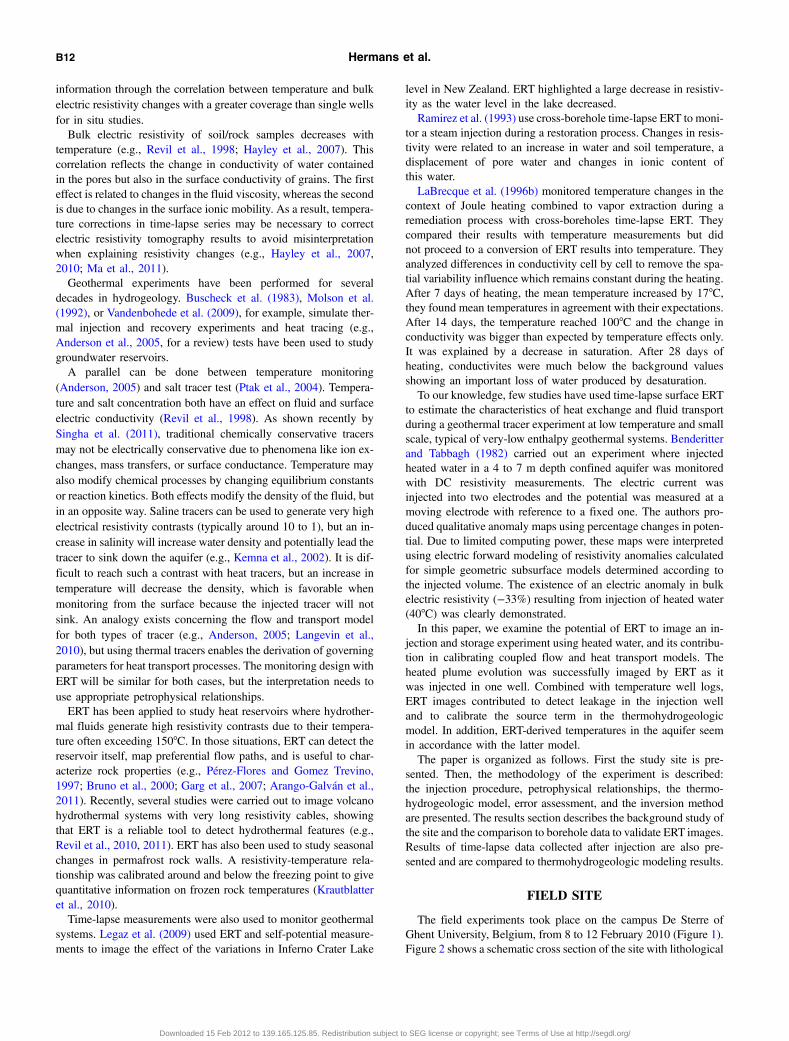
resistivity is detected at the well. At this time, the volume of heatedwater injected in the well was limited to 2.1 m3, yielding a smallanomaly that ERT can barely image. After 48 h (Figure 6b), theanomaly is enlarged and the change in resistivity is higher (−15%).Because the volume of heated water injected is doubled (4.2 m3),ERT managed to image the plume in more details. At the end ofinjection (Figure 6c), the decrease in resistivity reaches its maxi-mum (17%). The geophysical inversions show that the plume ex-tension is limited in depth by the clay layer. This result is also inaccordance with the hydrogeology of the site because this layer isconsidered as impermeable.A decrease of electric resistivity is observed above the top of the

screen in the aquifer, between −2 and −3.5 m, where thebentonite seal was placed. This variation corresponds to an increasein temperature, as shown by temperature logs (Figure 8) carried outafter the injection phase (Vandenbohede et al., 2011). Such animportant increase in temperature could not be explained onlyby heating due to thermal conduction from the PVC casing (thermalconductivity of 0.17 W∕mC°). This phenomenon can be explainedif the bentonite seal used to prevent leakage of injection water wasnot properly set up, inducing injection of heated water to reach theupper part of the aquifer. Another hydraulic conductivity anisotropyratio, with a greater vertical component, could have a similar effect.However, even a forward flow and transport simulation with a 1∶1

5 10 15 20 25 30 35 40 45

–10

–5

–7 –6 –5 –4 –3 –2 –1

5 10 15 20 25 30 35 40 45

–10

–5

log S

Distance along the profile (m)

10–510–410–310–210–1100–10

–9

–8

–7

–6

–5

–4

–3

–2

–1

0

Relative cumulative sensitivity

Dep

th (

m)

Dep

th (

m)

Dep

th (

m)

Background

Time-lapse

Clay limit

sensitivity log

a)

b)

c)

Figure 7. The cumulative sensitivity before the test (a) and duringthe test (b) remain similar in the zone of injection (between −2 and−4.5 m), artifacts due to different resolutions should be avoided. Alog of sensitivity at the position of the well (c) enabled to appreciatequantitatively this similarity. The maximum difference in the zoneof injection is found at the bottom of the sand where the sensitivityis 8 × 10−3 for the background and 5 × 10−3 after 48 hours.

10 20 30 40 50–5

–4

–3

–2

Well water temperature (°C)

Dep

th (

m)

0.2 d1.9 d4

d5d

6d

9.9

d11

.9d

14d

17d

21d

26d

32.9

d41

.9d

Figure 8. Temperature logs were taken after the injection in the in-jection well (W01) to control the temperature in the aquifer and tocalibrate the thermohydrogeologic model. The misfit betweenobserved (o) and calculated (solid line) temperature logs can be ap-preciated at different observation times (Vandenbohede et al, 2011).

B18 Hermans et al.

Downloaded 15 Feb 2012 to 139.165.125.85. Redistribution subject to SEG license or copyright; see Terms of Use at http://segdl.org/

anisotropy ratio is not able to produce temperatures similar to theone observed with the logs. We thus favor the former hypothesis. Inaddition, we observe a bulk electric resistivity decrease in the un-saturated zone along the well, which could be caused by thermalconduction through the pipe.On Figure 6a and 6b, we see an almost systematic lowering of

5% in bulk electric resistivity across the entire image. In contrast,in Figure 6c, significant changes are limited to the zone of injec-tion; elsewhere, variations are around −3% at maximum. It is im-portant to recall that all the inversions were run with the samelevel of noise, determined once with the reciprocal error. However,we think that the data quality (noise level), which was estimatedonly once after the injection, varied during the three days of in-jection (e.g., Miller et al., 2008). During the background, theweather was dry with air temperature above 0°C. For the follow-ing two days, air temperature decreased below 0°C and snow fell.Surface conditions were thus completely different, which influ-enced the contact resistance at electrodes and therefore the noiselevel. This change might affect the overall quality of the imagealso at depth and might be reflected in the difference inversionthrough enhanced/reduced smoothing effect. As a result, the−10% isoline seems larger after 48 h than after 72 h. At theend of injection, temperature was again above zero and weatherconditions were closer to that of the background.To assess the minimal changes in temperature that could be

detected by the electric survey, which depends mainly on the elec-tric resistivity distribution, on the estimated S/N and on the arraydesign, we generated an ensemble of 100 geoelectric data setsby adding a 2.5% Gaussian random noise to the field data thatwas used to compute the background image (Figure 5). This ensem-ble was then inverted with the same inversion parameters (Kemnaet al., 2007). We found that the distribution of each parameter fol-lows a Gaussian distribution. The generated artificial electric resis-tivity changes are around 3% to 5%, when considering changesbetween the average resistivity and the average resistivity minusone standard deviation. This would correspond to temperature var-iations of about 2°C to 3°C. As a result, we considered only changestwo times greater than the noise-related changes (10% in magni-tude) as significant.An anomaly is also present at 37 m from the beginning of the

profile. At this position, a big tree was present. Barker and Moore(1998) show the influence of roots in the saturation of sands and thistree could explain why resistivities below 100 ohm-m are found lessdeep than elsewhere in the section (Figure 5). However, the cause ofthe 10% decrease in resistivity below the water table at this positionis unclear.

Comparison with thermohydrogeologic modeling

In our initial modeling attempt, the injection rate was concen-trated at the screen position. To account for the geophysical obser-vations, which shows a temperature increase all along the well, itwas necessary to spread the injection rate over the complete lengthof the well in the thermohydrogeologic model. Figure 8 shows, insupport of the geophysical images, increased temperatures in theinjection well, corresponding to downhole temperature profiles,above the screen during the storage phase, reflecting the failureof the bentonite to seal the annular space of the well. We assumethat these temperatures are in equilibrium with water outside of the

borehole. The results of the calibration process are presented inTable 1.Resistivity values from ERT images were converted into tempera-

ture using equations 1 and 3 (called hereafter ERT-derived tempera-ture). The main difficulty was to account for the difference inelectric conductivity of formation water and tap water. To do so,we used the simulation from the calibrated model during theinjection phase (see section Methods). It was then possible to com-pare our ERT results with the thermohydrogeologic model.The comparison (Figure 9) shows that the horizontal and

vertical positions of the plume after 72 h are correctly imaged,but the plume itself is enlarged. Before 72 h, the volume of heatedwater is not big enough to be correctly imaged (not shown here).The enlargement of the plume can be easily explained by thesmoothness constraint used to regularize the model differences inthe inversion process and was also observed by Vanderborght et al.(2005) for a saline tracer.The ERT-derived temperature image also shows changes near the

surface in the unsaturated zone, between 0 and –2 m depth. Here,saturation variations can also explain smaller resistivity values. Thetemperature values given in Figure 9b in the unsaturated zone arenot reliable because they assume similar saturations for the back-ground and the time-lapse series.Temperatures monitored with ERT are quite consistent with the

thermohydrogeologic modeling after 72 h. The maximumtemperature deduced from ERT is 45°C which is only 3°C belowthe mean temperature of injection. The width and thickness ofthe plume are also satisfactory. Note that the smoothing effect ofthe regularization is in part counterbalanced by the spatial distribu-tion of the proportion of tap and formation water obtained fromhydrogeologic simulations.

Figure 9. Petrophysical laws enabled to transform resistivity valuesinto temperatures. The plume detected with ERT (b) is in accor-dance with the plume calculated with a calibrated thermohydrogeo-logic model (a).

Shallow geothermal test monitored with ERT B19

Downloaded 15 Feb 2012 to 139.165.125.85. Redistribution subject to SEG license or copyright; see Terms of Use at http://segdl.org/

CONCLUSION

Electric resistivity tomography appears to be a reliable tool toimage injection and storage of heated water and should thereforebe further studied to complement thermal response tests. Wemapped the extent of a geothermal plume around a borehole, in un-favorable field conditions (varying surface conditions). Changes inresistivity can be interpreted qualitatively to follow the evolution ofthe plume of heated water in the subsurface and quantitatively toestimate the temperature change. At shallow depths, ERT was ableto detect leakage in the bentonite seal and appears as a reliable toolto check in situ geothermal installations, their efficiency and pos-sible heat losses.Laboratory measurements and site specific petrophysical rela-

tionships enabled quantitative interpretation in terms of temperaturein the aquifer. Such volumetric information, in contrast with tem-perature logs, could be of great importance to calibrate thermohy-drogeologic models, which often rely on integrated and localizedinformation to calibrate volumetric parameters. In our specific case,the difference in conductivity between formation and injectionwaters limited the use of inferred temperature directly in the ther-mohydrogeologic model, even if they appear to be reliable. How-ever, geophysics was used to conceptualize the source term of thethermohydrogeologic model. At present, few techniques address thein situ characterization of low enthalpy geothermal systems and aspecific methodology could be developed including ERT and othergeophysical methods sensitive to temperature changes.A limitation to quantify directly hydrogeologic and heat transport

parameters with ERT results seems to be the regularization methodused to invert the data. It could be interesting to combine forwardelectric modeling and hydrogeologic modeling in a coupled-inversion scheme to avoid the regularization, and thus thesmoothing.A second main disadvantage is the loss of resolution with depth.

For deeper geothermal reservoirs, crosshole tomography could beapplied to image the temperature distribution in the reservoir. Weimaged correctly with surface ERT measurements a 35°C tempera-ture change, corresponding to a decrease of 17% in bulk electricresistivity, using an electrode spacing a of 0.75 m, a 2.5-m-thick,3-m-width, and 3-m deep hot water plume. We can generalize thesefeatures using nondimensional numbers linked to the electrode spa-cing a: thickness of 3.33a, width and depth of 4a. These valuescan serve as guidelines for further studies and application to deeperreservoirs.The road ahead is to perform a more quantitative integration of

our geophysical data and results in the thermohydrogeologic mod-eling, if modeling is performed, and to refine the geophysical ima-ging, if imaging is needed. Our approach should, in time, contributeto the development of in situ techniques to characterize groundwaterand porous matrix properties governing heat transfer in the subsur-face and to monitor shallow geothermal resources exploitation.

ACKNOWLEDGMENTS

We would like to thank the Fund for Scientific Research for sup-porting Thomas Hermans (French Community) as an aspirant andAlexander Vandenbohede (Flanders) as a postdoctoral researcher.We also thank the “Bourse Pisart” of Liege University for givingfunds for the internship of Thomas Hermans in Ghent University.We would like to thank deeply the editor Vladimir Grechka and the

associate editor for motivating us in improving the manuscript sinceits first version. We thank A. Revil, L.R. Bentley, and an anon-ymous reviewer for their constructive remarks leading to a greatlyimproved manuscript.

REFERENCES

Allen, A., and D. Milenic, 2003, Low-enthalpy geothermal energy resourcesfrom groundwater in fluvioglacial gravels of buried valleys: AppliedEnergy, 74, 9–19, doi: 10.1016/S0306-2619(02)00126-5.

Alumbaugh, D. L., and G. A. Newman, 2000, Image apraisal for 2-D and3-D electromagnetic inversion: Geophysics, 65, 1455–1467, doi:10.1190/1.1444834.

Anderson, M. P., 2005, Heat as a ground water tracer: Ground Water, 43,951–968, doi: 10.1111/gwat.2005.43.issue-6.

Arango-Galván, C., R. M. Prol-Ledesma, E. L. Flores-Márquez, C. Canet,and R. E. Villanueva Estrada, 2011, Shallow submarine and subaerial,low-enthalpy hydrothermal manifestations on Punta Banda, BajaCalifornia, Mexico: Geophysical and geochemical characterization:Geothermics, 40, 102–111, doi: 10.1016/j.geothermics.2011.03.002.

Archie, G. E., 1942, The electrical resistivity log as an aid in determiningsome reservoir characteristics: Association for Computing Machinery,Transactions on Mathematical Software, 146, 54–62.

Aster, R. C., B. Borchers, and C. Thurber, 2005, Parameter estimation andinverse problems: Elsevier Academic Press.

Barker, R., and J. Moore, 1998, The application of time-lapse electricaltomography in groundwater studies: The Leading Edge, 17,1454–1458, doi: 10.1190/1.1437878.

Benderitter, Y., and J. Tabbagh, 1982, Heat storage in a shallow confinedaquifer: Geophysical tests to detect the resulting anomaly and its evolutionwith time: Journal of Hydrology, 56, 85–98, doi: 10.1016/0022-1694(82)90058-0.

Bentley, L. R., and M. Gharibi, 2004, Two- and three-dimensional electricalresistivity imaging at a heterogeneous remediation site: Geophysics, 69,674–680, doi: 10.1190/1.1759453.

Bolève, A., A. Crespy, A. Revil, F. Janod, and J. L. Mattiuzzo, 2007, Stream-ing potentials of granular media: Influence of the Duhkin and Reynoldsnumbers: Journal of Geophysical Research, 112, B08204, doi: 10.1029/2006JB004673.

Bowling, J. C., D. L. Harry, A. B. Rodriguez, and C. Zheng, 2007, Integratedgeophysical and geological investigation of a heterogeneous fluvial aqui-fer in Columbus, Mississippi: Journal of Applied Geophysics, 62, 58–73,doi: 10.1016/j.jappgeo.2006.08.003.

Bruno, P. P. G., V. Paoletti, M. Grimaldi, and A. Rapolla, 2000, Geophysicalexploration for geothermal low enthalpy resources in Lipari Island, Italy:Journal of Volcanology and Geothermal Research, 98, 173–188, doi:10.1016/S0377-0273(99)00183-3.

Busby, J., M. Lewis, H. Reeves, and R. Lawley, 2009, Initial geologicalconsiderations before installing ground source heat pump systems:Quarterly Journal of Engineering Geology and Hydrogeology, 42,295–306.

Buscheck, T. A., C. Doughty, and C. F. Tsang, 1983, Prediction and analysisof a field experiment on a multilayered aquifer thermal energy storagesystem with strong buoyancy flow: Water Resources Research, 19,1307–1315, doi: 10.1029/WR019i005p01307.

Butler, J. J., 1998, The design, performance, and analysis of slug tests: LewisPublishers.

Dahlin, T., and B. Zhou, 2004, A numerical comparison of 2D resistivityimaging with ten electrode arrays: Geophysical Prospecting, 52,379–398, doi: 10.1111/gpr.2004.52.issue-5.

deGroot-Hedlin, C., and S. Constable, 1990, Occam’s inversion to generatesmooth, two dimensional models from magnetotelluric data: Geophysics,55, 1613–1624, doi: 10.1190/1.1442813.

Garg, S. K., J. W. Pritchett, P. E. Wannamaker, and J. Combs, 2007, Char-acterization of geothermal reservoirs with electrical surveys: Beowavegeothermal field: Geothermics, 36, 487–517, doi: 10.1016/j.geothermics.2007.07.005.

Harbaugh, A. W., E. R. Banta, M. C. Hill, and M. G. McDonald, 2000,MODFLOW-2000, the U.S. Geological Survey modular ground-watermodel: User guide to modularization concepts and the ground-water pro-cess, USGS Open-File Rep, 00-92.

Hayashi, M., 2004, Temperature-electrical conductivity relation of water forenvironmental monitoring and geophysical data inversion: EnvironmentalMonitoring and Assessment, 96, 119–128, doi: 10.1023/B:EMAS.0000031719.83065.68.

Hayley, K., L. R. Bentley, M. Gharibi, and M. Nightingale, 2007, Low tem-perature dependence of electrical resistivity: Implications for near surfacegeophysical monitoring: Geophysical Research Letters, 34, L18402, doi:10.1029/2007GL031124.

B20 Hermans et al.

Downloaded 15 Feb 2012 to 139.165.125.85. Redistribution subject to SEG license or copyright; see Terms of Use at http://segdl.org/

Hayley, K., L. R. Bentley, and A. Pidlisecky, 2010, Compensating fortemperature variations in time-lapse electrical resistivity difference ima-ging: Geophysics, 75, no. 4, WA51–WA59, doi: 10.1190/1.3478208.

Hyder, Z., J. J. Butler, C. D. McElwee, and W. Liu, 1994, Slug tests inpartially penetrating wells: Water Resources Research, 30, 2945–2957,doi: 10.1029/94WR01670.

Jardani, A., A. Revil, W. Barrash, A. Crespy, E. Rizzo, S. Straface,M. Cardiff, B. Malama, C. Miller, and T. Johnson, 2009, Reconstructionof the water table from self-potential data: A Bayesian approach: GroundWater, 47, 213–227, doi: 10.1111/gwat.2009.47.issue-2.

Kaipio, J. P., V. Kolehmainen, M. Vauhkonen, and E. Somersalo, 1999,Inverse problems with structural prior information: Inverse Problems,15, 713–729, doi: 10.1088/0266-5611/15/3/306.

Keller, G. V., and F. C. Frischknecht, 1966, Electrical methods ingeophysical prospecting: Oxford.

Kemna, A., 2000, Tomographic inversion of complex resistivity — Theoryand application: Ph.D. thesis, Ruhr-University of Bochum.

Kemna, A., F. Nguyen, and S. Gossen, 2007, On linear model uncertaintycomputation in electrical imaging: SIAM Conference on mathematicaland computational issues in the Geosciences, 82.

Kemna, A., J. Vanderborght, B. Kulessa, and H. Vereecken, 2002, Imagingand characterization of subsurface solute transport using electricalresistivity tomography (ERT) and equivalent transport models: Journalof Hydrology, 267, 125–146, doi: 10.1016/S0022-1694(02)00145-2.

Krautblatter, M., S. Verleysdonk, A. Flores-Orozco, and A. Kemna, 2010,Temperature-calibrated imaging of seasonal changes in permafrost rockwalls by quantitative electrical resistivity tomography (Zugspitze,German/Austrian Alps): Journal of Geophysical Research, 115,F02003, doi: 10.1029/2008JF001209.

LaBrecque, D. J., M. Miletto, W. Daily, A. Ramirez, and E. Owen, 1996a,The effects of noise on Occam’s inversion of resistivity tomography data:Geophysics, 61, 538–548, doi: 10.1190/1.1443980.

LaBrecque, D. J., A. L. Ramirez, W. D. Daily, A. M. Binley, andS. A. Schima, 1996b, ERT monitoring of environmental remediation pro-cesses: Measurement Science and Technology, 7, 375–383, doi: 10.1088/0957-0233/7/3/019.

LaBrecque, D. J., and X. Yang, 2000, Difference inversion of ERT data: Afast inversion method for 3-D in-situ monitoring: Proceedings SAGEEP,723–732.

Langevin, C. D., A. M. Dausman, and M. C. Sukop, 2010, Solute and heattransport model of the Henry and Hilleke laboratory experiment: GroundWater, 48, 757–770, doi: 10.1111/j.1745-6584.2009.00596.x.

Langevin, C. D., D. T. Thorne, A. M. Dausman, M. C. Sukop, andW. Guo, 2007, SEAWAT Version 4: A computer program for simulationof multi-species solute and heat transport, U.S. Geolological SurveyTechnical Methods, Book 6, chap. A22.

Lebbe, L., M. Mahouden, and W. De Breuck, 1992, Execution of a triplepumping test and interpretation by an inverse numerical model: AppliedHydrogeology, 4, 20–34.

Legaz, A., J. Vandenmeulebrouck, A. Revil, A. Kemna, A. W. Hurst, R.Reeves, and R. Papasin, 2009, A case study of resistivity and self-potential signatures of hydrothermal instabilities, Inferno Crater Lake,Waimangu, New Zealand: Geophysical Research Letters, 36, L12306,doi: 10.1029/2009GL037573.

Leroy, P., A. Revil, A. Kemna, P. Cosenza, and A. Ghorbani, 2008, Complexconductivity of water-saturated packs of glass beads: Journal of Colloidand Interface Science, 321, 103–117, doi: 10.1016/j.jcis.2007.12.031.

Lund, J. W., 2010, Direct utilization of geothermal energy: Energiespectrum,3, 1443–1471, doi: 10.3390/en3081443.

Lund, J. W., D. H. Freeston, and T. L. Boyd, 2005, Direct applicationof geothermal energy: 2005 worldwide review: Geothermics, 34,691–727, doi: 10.1016/j.geothermics.2005.09.003.

Ma, R., A. McBratney, B. Whelan, B. Minasny, and M. Short, 2011,Comparing temperature correction models for soil electrical conductivitymeasurement: Precision Agriculture, 12, 55–66.

Miller, C. R., P. S. Routh, T. R. Brosten, and J. P. McNamara, 2008,Application of time-lapse ERT imaging to watershed characterization:Geophysics, 73, no. 3, G7–G17, doi: 10.1190/1.2907156.

Molson, J. W., E. O. Frind, and C. D. Palmer, 1992, Thermal energy storagein an unconfined aquifer: 2. Model development, validation, and applica-tion: Water Resources Research, 28, 2857–2867, doi: 10.1029/92WR01472.

Nguyen, F., A. Kemna, A. Antonsson, P. Engesgaard, O. Kuras, R. Ogilvy,J. Gisbert, S. Jorreto, and A. Pulido-Bosch, 2009, Characterization ofseawater intrusion using 2D electrical imaging: Near Surface Geophysics,7, 377–390.

Parasnis, D. S., 1988, Reciprocity theorems in geoelectric and geoelectro-manetic work: Geoexploration; International Journal of Mining andTechnical Geophysics and Related Subjects, 25, 177–198, doi:10.1016/0016-7142(88)90014-2.

Pérez Flores, M. A., and E. Gomez Trevino, 1997, Dipole-dipole resistivityimaging of the Ahuachapan-Chipilapa geothermal field, El Salvador:Geothermics, 26, 657–680, doi: 10.1016/S0375-6505(97)00015-1.

Ptak, T., M. Piepenbrink, and E. Martac, 2004, Tracer tests for the investiga-tion of heterogeneous porous media and stochastic modelling of flow andtransport — A review of some recent developments: Journal of Hydrol-ogy, 294, 122–163, doi: 10.1016/j.jhydrol.2004.01.020.

Ramirez, A., W. Daily, D. LaBrecque, E. Owen, and D. Chesnut, 1993,Monitoring an underground steam injection process using electrical resis-tance tomography: Water Resources Research, 29, 73–87, doi: 10.1029/92WR01608.

Revil, A., L. M. Cathles, S. Losh, and J. A. Nunn, 1998, Electrical conduc-tivity in shaly sands with geophysical applications: Journal of Geophy-sical Research, 103, 23925–23936, doi: 10.1029/98JB02125.

Revil, A., A. Finizola, T. Ricci, E. Delcher, A. Peltier, S. Barde-Cabusson,G. Avard, T. Bailly, L. Bennati, S. Byrdina, J. Colonge, F. Di Ganga,G. Douillet, M. Lupi, J. Letort, and E. Tsang Hin Sun, 2011, Hydrogeol-ogy of Stromboli volcano, Aeolian Islands (Italy) from the interpretationof resistivity tomograms, self-potential, soil temperature and soil CO2concentration measurements: Geophysical Journal International, 186,1078–1094, doi: 10.1111/j.1365-246X.2011.05112.x.

Revil, A., T. C. Johnson, and A. Finizola, 2010, Three-dimensionalresistivity tomography of Vulcan’s Forge, Vulcano Island, southernItaly: Geophysical Research Letters, 37, L15308, doi: 10.1029/2010GL043983.

Revil, A., and N. Linde, 2006, Chemico-electrochemical coupling in micro-porous media: Journal of Colloid and Interface Science, 302, 682–694,doi: 10.1016/j.jcis.2006.06.051.

Revil, A., H. Schwaeger, L. M. Cathles, and P. D. Manhardt, 1999, Stream-ing potential in porous media 2. Theory and application to geothermalsystems: Journal of Geophysical Research, 104, 20033–20048, doi:10.1029/1999JB900090.

Singha, K., and S. M. Gorelick, 2006, Effects of spatially variable resolutionon field-scale estimates of tracer concentration from electrical inversionsusing Archie’s law: Geophysics, 71, no. 3, G83–G91, doi: 10.1190/1.2194900.

Singha, K., L. Li, F. D. Day-Lewis, and A. B. Regberg, 2011, Quantifyingsolute transport processes: Are chemically “conservative” tracers electri-cally conservative?: Geophysics, 76, no. 1, F53–F63, doi: 10.1190/1.3511356.

Slater, L., A. M. Binley, W. Daily, and R. Johnson, 2000, Cross-hole elec-trical imaging of a controlled saline tracer injection: Journal of appliedgeophysics, 44, 85–102, doi: 10.1016/S0926-9851(00)00002-1.

Suzuki, S., 1960, Percolation measurements based on heat flow through soilwith special reference to paddy fields: Journal of Geophysical Research,65, 2883–2885, doi: 10.1029/JZ065i009p02883.

Tikhonov, A. N., and V. A. Arsenin, 1977, Solution of ill-posed problems:Winston & Sons.

Vandenbohede, A., T. Hermans, F. Nguyen, and L. Lebbe, 2011, Shallowheat injection and storage experiment: Heat transport simulation and sen-sitivity analysis: Journal of Hydrology, 409, 262–272, doi: 10.1016/j.jhydrol.2011.08.024.

Vandenbohede, A., and L. Lebbe, 2002, 3D density dependent numericalmodel of a tracer test performed in the Belgian coastal plain: Proceedingof the First Geologica Belgica International Meeting, Aardkundige Me-dedelingen, 12, 223–226.

Vandenbohede, A., and L. Lebbe, 2003, Combined interpretation of pump-ing and tracer tests: Theoritical considerations and illustration with a fieldtest: Journal of Hydrology, 277, 134–149, doi: 10.1016/S0022-1694(03)00090-8.

Vandenbohede, A., and L. Lebbe, 2006, Double forced gradient tracer test:Performance and interpretation of a field test using a new solute transportmodel: Journal of Hydrology, 317, 155–170, doi: 10.1016/j.jhydrol.2005.05.015.

Vandenbohede, A., A. Louwyck, and L. Lebbe, 2009, Conservative soluteversus heat transport in porous media during push-pull tests: Transport inPorous Media, 76, 265–287, doi: 10.1007/s11242-008-9246-4.

Vanderborght, J., A. Kemna, H. Hardelauf, and H. Vereecken, 2005, Poten-tial of electrical resistivity tomography to infer aquifer transport charac-teristics from tracer studies: A synthetic case study: Water ResourcesResearch, 41, W06013, doi: 10.1029/2004WR003774.

Waxman, M. H., and L. J. M. Smits, 1968, Electrical conductivities in oil-bearing shaly sands: Society of Petroleum Engineers Journal, 8, 107–122,doi: 10.2118/1863-A.

Zheng, C., and P. P. Wang, 1999, MT3DMS, a modular three-dimensionalmultispecies model for simulation of advection, dispersion and chemicalreactions of contaminants in groundwater systems: Documentation anduser’s guide, U.S. Army Engineer Research and Development CenterContract Report SERDP-99-1.

Shallow geothermal test monitored with ERT B21

Downloaded 15 Feb 2012 to 139.165.125.85. Redistribution subject to SEG license or copyright; see Terms of Use at http://segdl.org/