Embed Size (px)
Citation preview
A set of canonical problems in sloshing. Part 0: Experimental setup and data processing A. Souto-Iglesias a'*, E. Botia-Vera a, A. Martín b, F. Pérez-Arribas a
a Naval Architecture Department (ETSIN), Technical University of Madrid (UPM), 28040 Madrid, Spain b University Institute for Automobile Research (INSIA), Technical University of Madrid (UPM), 2803Í Madrid, Spain
A R T I C L E I N F O A B S T R A C T
Keywords: Uncertainty analysis Sloshing Experimental data reconstructing
In a series of attempts to research and document relevant sloshing type phenomena, a series of experiments have been conducted. The aim of this paper is to describe the setup and data processing of such experiments. A sloshing tank is subjected to angular motion. As a result pressure registers are obtained at several locations, together with the motion data, torque and a collection of image and video information. The experimental rig and the data acquisition systems are described. Useful information for experimental sloshing research practitioners is provided. This information is related to the liquids used in the experiments, the dying techniques, tank building processes, synchronization of acquisition systems, etc. A new procedure for reconstructing experimental data, that takes into account experimental uncertainties, is presented. This procedure is based on a least squares spline approximation of the data. Based on a deterministic approach to the first sloshing wave impact event in a sloshing experiment, an uncertainty analysis procedure of the associated first pressure peak valué is described.
1. Introduction
This paper is part of a series of ongoing attempts to research and document relevant sloshing type phenomena, by means of mainly experimental techniques, with the aim of generating useful reference data for CFD validation. The relevant details of the experimental setups as well as the techniques used for the data processing are presented in this paper. A previously pub-lished paper (Delorme et al., 2009) was dedicated to the study of the influence of excitation frequency on wave impact pressures induced by lateral sloshing during roll motions. The following papers in the series will treat problems related to wave impact pressure statistical analysis and fluid structure interaction. The information obtained from this sloshing rig has been used for CFD validation in a number of recent papers (Khayyer and Gotoh, 2009; Bulian et al., 2010; Idelsohn et al., 2008; Degroote et al., 2010; Souto-Iglesias et al., 2006) but there is room for improve-ment in the reference data and progress in this direction is in the spirit of the present work.
Sloshing is the intense movement of the free surface of liquids inside tanks. It generates dynamic loads on the tank structure and thus becomes an important issue to be considered in the design and operation of membrane system LNG vessels (Tveitnes et al., 2004).
* Corresponding author. Tel.: +34 91 336 71 56; fax: +34 91 544 21 49. E-mail address: [email protected] (A. Souto-Iglesias).
At the moment, this phenomenon is receiving a lot of attention due to the ongoing conceptual design projects for floating LNG extraction and liquefaction plants (Kuo et al., 2009). As reported by stake-holders, it is foreseen that the SPB type tanks, for which no sloshing related risks are expected, will be the ones used for the FPSO permanent unit. Nonetheless, most of the LNG tankers fleet, which will have to offload the LNG from those units, belong to the membrane type, with a general arrangement of four or five large un-baffled containment tanks. Consequently, the risk of severe sloshing damages is high during the offloading operation, when these tanks remain partially filled.
The research on sloshing from the experimental point of view has been mainly led by classification societies like DNV, ABS or LRS. Obtaining a detailed description of these experiments is often difficult due to the confidentiality of these studies. Berg (1987) and Olsen (1976) both for DNV and Bass et al. (1985) studied the impact pressures in sloshing flows, as well as the very interesting and intricate issue of the scaling of sloshing experimental valúes to full scale. These studies suffered from limitations due to the limited recording and sampling capabilities of the data acquisition systems that were state of the art at that time. They were not capable of capturing high frequency modes in the pressure signáis ñor long series of data which was necessary to perform a rigorous probabilistic analysis.
The situation has evolved in the last 10 years from those seminal studies by incorporating recent data acquisition technol-ogies using one degree of freedom linear (Panigrahy et al., 2009;

Eswaran et al., 2009) and angular motion rigs (Akyildiz and Ünal, 2005) and six degrees of freedom platforms that allow the reproduc-tion of complex ship motions (Pistani et al., 2010). A very significant contribution belongs to Lugni et al. (2006, 2010a, 2010b), who described the extraordinary accelerations during wave impact events, though their work is not specifically arranged so as to be useful as reference for CFD validation attempts. A widely known attempt to provide such validation data emerged from the Special lst "Sloshing Dynamics" Symposium at ISOPE-2009 Conference in which a bench-mark test case was proposed to all participants (Kim et al., 2009).
Graczyk et al. (2006), Graczyk and Moan (2008) and Pastoor et al. (2005) have tried to characterize the sloshing related loads from a probabilistic assessment of extensive registers of sloshing cycles. Nonetheless, the probabilistic approach is of limited use for the validation of CFD simulations. Data from canonical well understood deterministic experiments provides better reference information for CFD validation. Based on the previous assumptions, we have thoroughly documented the experimental procedure that we have used and elaborated data treatment techniques that enable the use of sloshing experimental data in CFD simulations. A significant part of this attempt is grounded on the data fitting technique documented in this paper. This technique is based on a novel B-spline reconstruction of the time history of a certain experimental magni-tude obtained by fitting the experimental history with a constrained least-squares approximation. Reconstruction techniques are often used as a complement of PIV measurements (see e.g. Lu and Smith, 1991), but they are not that common when providing reference data for CFD validation. The approach is described in Section 3.3 and computer codes are provided as supplementary materials.
It is relevant to mention that the growing interest in the study of sloshing phenomena has not been complemented with developments in the estimation of the uncertainties associated with the experiments and actually the aforementioned proposed benchmark (Kim et al., 2009) lacks such analysis. Within this scenario, it seems reasonable to devote some effort to assess the
quality of experimental results in order to make them much more useful and risk-free when validating numerical results or more importantly when using them in Engineering. Quoting Stern et al. (1999), "Experimental uncertainty estimates are imperative for risk assessments in design both when using data directly or in calibrating and/or validating simulation methods".
To that extent, this work adapts the AIAA (1995) and ANSI/ASME procedures to estímate experimental uncertainties of sloshing type investigations. First, the essence of the problem is described, followed by a detailed explanation of how the experiment is carried out. First of all, the kind of problem for which the uncertainty analysis is desired is described, and then the procedure to be followed for a real test case will be documented. As aforementioned, the literature on uncertainty analysis on sloshing problems is scarce. There are a few seminal references on uncertainty analysis in the naval fie Id by the IIHR Iowa group (Gui et al., 2001 a,b, 2002; Longo and Stern, 2005; Stern et al., 1999), but to our knowledge none of them have dealt with the sloshing problem.
The paper is organized as follows: First, a description of the sloshing rig is given, together with the fluids used in the experiments and special attention is paid to the data acquisition systems. Second, the data post-processing is explained, followed by the uncertainty analysis implemented in the study of pressure peaks in wave impact events. Third, the reconstruction of experimental data taking into account experimental uncertainties is documented. Finally a conclusions summary together with future work targets is provided.
2. Experimental setup
2.2. Testing rig
The testing rig is shown in Fig. 1. The driving system is a crank-rocker mechanism that transforms the rotational motion of an
Fig. 1. Angular motion sloshing rig case study.

1825
electric motor (element 10 in Fig. 1) into a harmonic rolling motion of the moving part of the rig (elements 1, 2,13 in Fig. 1) at the front. This moving part is designed to embrace a partially filled tank. The shaft which transmits the movement to the tank is adapted to measure torque and angular position by means of an encoder and a torquemeter, as seen in Fig. 1. The rocker (element 9 in Fig. 1) can be attached to the crank (element 11 in Fig. 1) at different positions making it possible to change the amplitude of the roll motion from 2o to 15°. Although differently dimensioned, the underlying concept of the testing rig is similar to the one used by Akyildiz and Ünal (2005). The harmonic rolling motion of the rocker is transmitted to the moving part of the rig through a torque transducer with a máximum rated torque of 200 Nm (element 3 in Fig. 1). Prior to A/D conversión, the torque signal is amplified using element 8 in Fig. 1. The máximum roll frequency is around 2 Hz. This depends mainly on the admissible torque which is influenced by the center of gravity, center of rotation and inertia of all the components. An incremental rotary optical encoder (element 4 in Fig. 1) registers the roll angle at the roll shaft.
The upper and lower arms (elements 1 and 2 in Fig. 1, respec-tively) of the moving part of the rig can be displaced along a vertical linear guide (element 13 in Fig. 1). This allows easy modification of the vertical position of the tank from one test to another. The bottom arm has two side telescopic supplements which are designed to easily hold tanks of different breadths. In conjunction with the shaft encoder at the lower end of the linear guide, a 25 pulses per millimeter linear incremental wire encoder (element 7 in Fig. 1) has been connected in order to increase the accuracy of the harmonic rolling motion monitoring.
The angular speed control is carried out with a frequency inverter (element 12 in Fig. 1) which controls the movement of the electric motor (element 10 in Fig. 1), which in turn governs the frequency of the shaft oscillation. The harmonic movement induced by the shaft is transmitted to the fluid motion inside the tank. The waves produced inside the tank hit the tank walls generating high pressures on them, which are measured by piezo-resistive pressure gauges (element 6 in Fig. 1). The pressure signal is amplified using element 5 in Fig. 1 before the A/D conversión. A reference zero position is defined by a locking handle (element 15 in Fig. 1). This item guarantees that the initial position remains invariable throughout the testing. An optical LED (element 14 in Fig. 1) shows the start of the movement using the first pulse of the aforementioned shaft rotatory encoder. This LED is used to synchronize the video recording with the movement signal. The motion starts in most cases counter-clockwise, which corre-sponds to positive angles.
The tanks are manufactured with plexiglass and assembled with screws. The one used in the main part of the experiments is rectangular and was originally dimensioned as a 1/60 scaled model of a longitudinal section of a 138,000 m3 LNG tanker hold. Main dimensions are 900 mm in breadth and 520 mm in height. Side faces can be replaced by double 2X and half 0.5X thickness (lX=62mm).
2.2. Fluids
Three different fluids have been used in the experiments: water, sunflower oil and glycerin. They are considered Newtonian fluids and their physical properties are shown in Table 1. The Reynolds number Re ranges from O(102) to 0(105) thus covering four orders of magnitude. The Weber number is similar for the three fluids. In order to increase the contrast in pictures and videos, the fluids are dyed using Fluorescein (water and glycerin) or Riboflavin (oil).
Table 1 Physical properties (SI units) of the liquids and non-dimensional numbers. p for density, ¡i for the dynamic viscosity, v for the kinematic viscosity and a for surface tensión.
Liquids
Water
Oil
Glycerin
P
998
900
1261
¡i
8.94e-4
0.045
0.934
V
8.96e-7
5 e - 5
7 .4e-4
O"
0.0728
0.033
0.064
J?e
0(105)
0(103)
0(102)
We
OOO3)
OOO3)
ooo3)
2.3. Data acquisition
2.3.í. Sensors Both analog and digital sensors have been used (see Fig. 2). The
pressure sensors and the torque transducer, all based on strain gauge measurements, belong to the first group. KULITE pressure 5 psi mini sensors model Xtel-190(M) have been used due to their small size (5 mm diameter) and high natural frequency (over 150 kHz). We refer the reader to the company specification sheet for further details. The rotatory and linear position encoders belong to the second group.
2.3.2. Actuators The main actuator control is variable-frequency drive (VFD)
SEW MOVIDRIVE MD60A used to change the velocity of the electrical motor which stimulates the testing rig. The VFD can manage several excitation frequencies (0.1-3 Hz). The output signal (Volts) needed to control the VFD is generated by the card NI PCI6221 analog output channel.
2.3.3. Signal conditioning The measurements obtained with strain gauges (mV) need
amplification prior to the A/D converter. The sensor output range (typically 18-20 mV) has to be conditioned to match the input span of the A/D converter (typically - 1 0 to 10 V) in order to optimize the accuracy of the amplification operation. This is achieved by adjust-ing the valué of the amplifier gain. This procedure is performed in every set of measurements by calibrating the gain through pre-liminary experiments.
2.3.4. Data recording The acquisition card (NI PCI6221) that centralizes the signáis
coming from the sensors has múltiple analog channels, digital counters and multipurpose A/D, I/O channels, which are used for control purposes. It can measure up to 16 multiplexed mode pressure sensors at a frequency of 20 kHz per channel, which means that the time delay in A/D conversión depends on this sampling frequency. In this particular case it is less or equal than by 0.0005 s for all channels. Such a high frequency rate is necessary in order to capture the high frequency pressure peaks (Pistani et al., 2010). Linking all of these devices is achieved by using a LABVIEW application. The output information is later processed and managed using DIADEM.
The qualitative point of view of our phenomena is captured with photographic and video recording by two camera devices. One of them has the capability to capture high speed videos and the other one has the capability to take photographs with high shutter speed. In order to synchronize the movement signal with the high speed video camera, the control software turns on a LED light when the first digital pulse coming from the position encoder is registered. This indicates that the movement has started. The photographs are taken using a similar program.

PRESSURE GAUGE KULITE XTL-190
mV
O V DC SOU
KR-CEUM010 AMPLIFIER
24VOCSOURCE
CANON EOS 450 D REFLEX CAMERA
i FREC
!
CAMERA RELAY 5VDC ANALOGDIGITAL CONVERTER 16 BITS
SHUTTER
ECUENCYINVERTER SEW MDV 60-A °)
ANALOG OUTPUTS 0-10VDC
CASIO FX-1 HIGH SPEED CAMERA
NI PCI 6221 DIGITAL OUTPUTS
05V DC DIGITAL INPUT PULSE COUNTERS HOMEPOSITION LED
ELECTRIC MOTOR 400 V AC SEW EURODRIVE
L
| > ( o . F E
DIGITAL A,B,Z
I DIFERENTIAL TO RSE SIGNAL CONVERTER SN65LBC173A
SHAFT ENCODER HEIDENHAIN ROD 426
12 V DC SOURCI fc*i DIGITAL
A,8,Z
LINEAR ENCODER DPF HLS-S 500 J
Fig. 2. Sloshing rig data acquisition scheme.
3. Data processing
3.2. General
One relevant aspect to be clarified when describing an experimental setup is to what extent the data obtained from the experiments is subjected to uncertainties. Some of the sensors are nominally digital, whilst others are analog. Nonetheless, in order to process the information recorded by the latter, the amplified signal needs to be converted into digital by the corresponding A/D converter. Therefore, the experimental phe-nomenon is described by a set of discontinuous discrete numbers. This particularity is a well known restriction and in principie it does not pose a problem. Nevertheless, if part of that information is going to be used as input for a numerical model, there are usually requests regarding the differentiability class of the time functions obtained from experiments. Quite often, the sampled variables in the experiments are essentially differentiable. They only become discontinuous after the sampling process, as for instance with the continuous motion of the moving parts of the sloshing rig when sampled with a digital encoder. It is good practice to recover as much of the original signal as possible by performing a fitting within the limits imposed by the uncertainties of the measurements.
In view of all this, it is important to assess and hopefully bound the uncertainties that are present in our experiments. On the other hand it is also important to provide good quality reference data to be eventually used as input data for numerical simulations, taking into account both the uncertainties and the nature of the phenomena under study. This section is dedicated to both issues.
3.2. Uncertainty analysis
3.2.í. General The uncertainty assessment of the results is based on a series of
standards and norms recommended by AIAA Standard S-071 for the majority of engineering tests (AIAA, 1995) and by the ITTC Quality Manual Procedures (International-Towing-Tank-Conference, 1999). Under these guidelines, the total uncertainty U is the root sum square of the total bias (systematic component, B) and the random error (precisión component, P):
U¿=B¿+P¿ (1)
Since pressure at specific locations forms part of the experimental data of all tests, the procedure is applied here to pressure peaks valúes. To our knowledge there is no previous attempt referred in the literature to apply this methodology to pressure registers in sloshing tests.
3.2.2. Pressure peaks We are considering, in order to exemplify the uncertainty
assessment procedure, the first pressure peak in a lateral impact event (Fig. 3). According to Choi et al. (2010), a correct flush mounting of the pressure gauge reduces the incidence of ripples and undesirable secondary peaks in the pressure register. This correct flush mounting is something to which attention has been paid in the setup. If, however, múltiple peaks are registered within one cycle, only the highest one is considered for the uncertainty analysis. The experiment is repeated N times (N=100), resuming it after letting the fluid rest. This is done for a number of configura-tions, considering different fluids, filling levéis, tank widths (Fig. 4), roll frequency, etc. Some of these experiments have been presented

in reference (Botia-Vera et al., 2010) and an extensive analysis of the experiments' outcomes is being prepared for submission.
For the particular configuration discussed here, the filling level ratio is 18%, the amplitude of the motion is 4o and the roll period is 0.85 times the first sloshing period.
The pressure p is obtained by measuring the amplified voltage V from the sensor with the corresponding zero offset V0 and the calibration slope Ka (given by the manufacturer, 29.92 mb/V):
p = Ka(V-V0) (2)
The sensitivity coefficients corresponding to the terms in Eq. (2) are defined as
ev-. dp sv -Ka, QV¡¡:
dp
SVQ -Ka, eKa
dp
dKa •V-VQ (3)
The bias term in the uncertainty is computed using this coefficients as
BP = 8VBV + 0VoBVo + 0KaBKa (4)
The bias due to voltage is 0.01 V and the bias of Ka, as given by the sensor manufacturer, is 0.06 mb/V. The valué 6Ka depends on the
5 0 - -
40 --
30 --
G
Pressure Impact [mBar] Roll Position [deg]
- ^ ^ \ \ ^ ^ — i — i — i — h ^ p — t ^ — i — i -
i —-i^H *< i
0 0.5 1 1.5 2 2.5 3 3.5
Fig. 3. Pressure at sensor one for the first peak in a lateral impact event.
specific test. In the test under consideration this valué is 1.1 V. Therefore Bp = 0.43 mb.
The average peak pressure p is obtained averaging the peaks of all the registers:
p = ^ L i P i v N
(5)
The precisión limit for this average is obtained from AIAA (1995)
(6)
with Sp the standard deviation of the sample, and tN_-¡ the Student coefficient with N - l degrees of freedom corresponding to the 95% confidence interval ( t=2 forN > 10). No exclusión criteria such as Chauvenet's has been considered; the experiments are performed in a rather isolated environment and we think there are no grounds to discard any measurement. For the sample
test case, p-. Therefore,
= 37.10 mb, S„ = 7.32mb, N=100, and P„ = 1.45mb.
Uj=BJ+PJ=2.28mb2
These results are summarized in Table 2. The ratio between the uncertainty Up and the average peak p is around 4% which is reasonably low enough to consider this data useful for CFD validations, regarding the computations of pressure peaks averages for initial conditions within the uncertainty ranges considered.
Table 2 Sample pressure peak valué and uncertainties.
V Up Bp Pp Up/P (%) &plU¡ (%) P¡/U¡ (%)
37.10 mb 1.51 mb 0.43 mb 1.45 mb 4.07 8.03
91.97
Fig. 4. First lateral impact event for three tank widths.
3.3. Experimental data reconstruction
3.3.í. General The experimental setup used in this series of studies provides an
accurate description of the angular motion of the tank. In principie, these real time-angle curves can be introduced directly as input data in any computational model aimed at having a consistent simulation of the experimental phenomena. Proceeding this way, when over-lapping experimental videos of sloshing flows and those of simula-tions, a sense of the quality of the simulation can be directly appreciated (Souto-Iglesias et al., 2006). In angular motions, the simplest initial condition is starting with a zero angle and zero angular velocity. The engine driving system of the rig is designed to produce a sinusoidal type motion in the tank. The engine drives a total mass composed not only of the liquid inside the tank but also of the tank itself as well as the structure that holds it. Therefore, it is physically unfeasible to achieve a sine motion instantaneously, and the real motion will have an initial zero angular velocity instead of finite speed, as in the sinusoidal case.
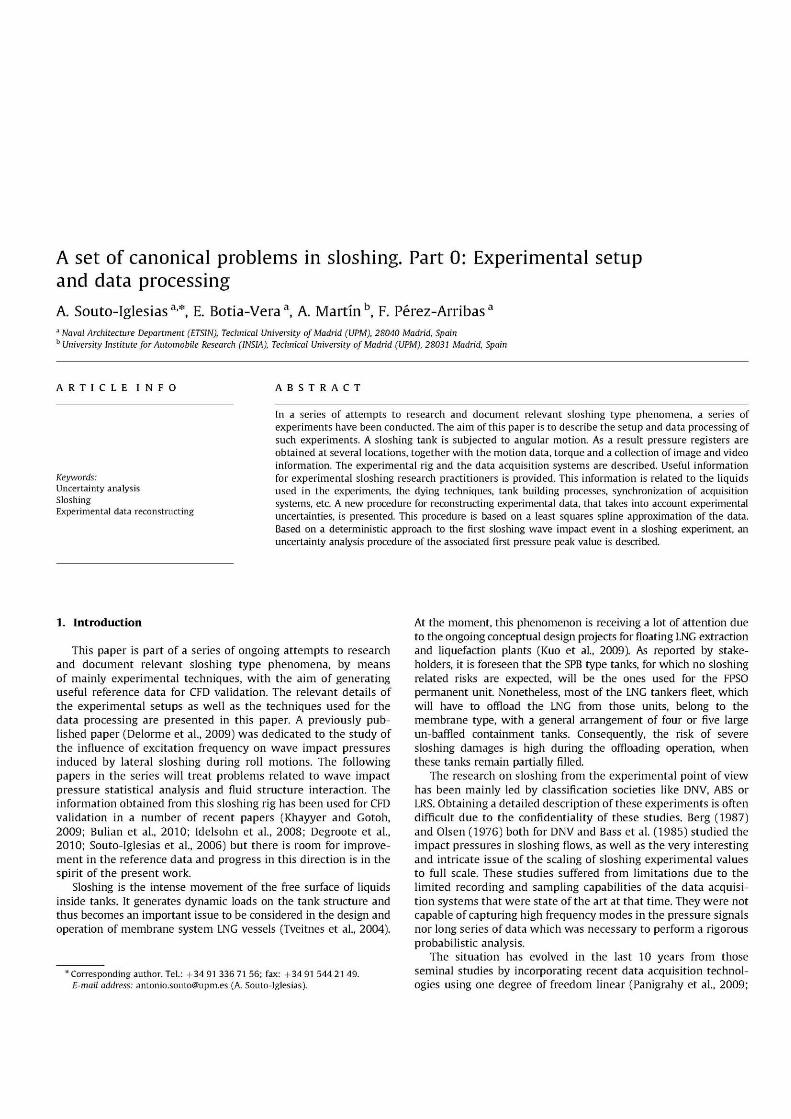
The angular position is measured using a 5000 pulses encoder with a precisión of 0.072°. It could appear to the reader that a 5000 holes encoder sensor is an adequate equipment to register the tank motion. Nevertheless, when dealing with + 2° amplitude roll motion, which is the mínimum the system can develop, such precisión error implies a relative error of 1.8%. The magnitude is twice this valué if we refer to just one part of the motion, either negative or positive angles. As a matter of fact, this error is not allowed if we want to use the encoder register to trigger a photographic camera or any real-time device. Moreover, when the angular measurement of that encoder is used to define the roll motion, a curve such as the one in Fig. 5 is obtained. This representation is discontinuous and inadequate to be used as the driving motion in a simulation code. It is not just a problem of the position itself, but of this position being used to estímate the roll angle derivatives, which are often needed to incorpórate inertia terms into the computational model (see e.g. Bulian et al., 2010), or to impose solid boundary conditions.
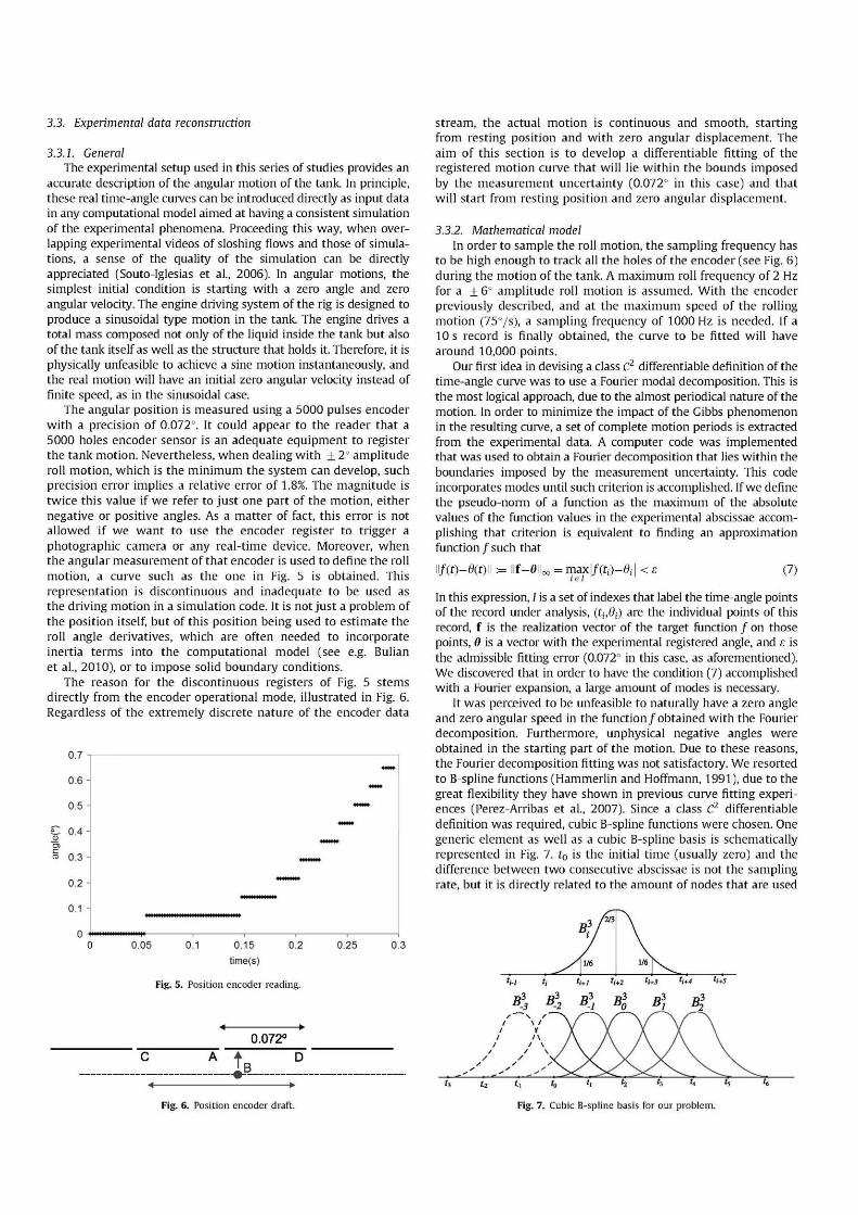
The reason for the discontinuous registers of Fig. 5 stems directly from the encoder operational mode, illustrated in Fig. 6. Regardless of the extremely discrete nature of the encoder data
Fig. 5. Position encoder reading.
0.072° A tF
stream, the actual motion is continuous and smooth, starting from resting position and with zero angular displacement. The aim of this section is to develop a differentiable fitting of the registered motion curve that will lie within the bounds imposed by the measurement uncertainty (0.072° in this case) and that will start from resting position and zero angular displacement.
3.3.2. Mathematical model In order to sample the roll motion, the sampling frequency has
to be high enough to track all the holes of the encoder (see Fig. 6) during the motion of the tank. A máximum roll frequency of 2 Hz for a + 6° amplitude roll motion is assumed. With the encoder previously described, and at the máximum speed of the rolling motion (75°/s), a sampling frequency of 1000 Hz is needed. If a 10 s record is finally obtained, the curve to be fitted will have around 10,000 points.
Our first idea in devising a class C2 differentiable definition of the time-angle curve was to use a Fourier modal decomposition. This is the most logical approach, due to the almost periodical nature of the motion. In order to minimize the impact of the Gibbs phenomenon in the resulting curve, a set of complete motion periods is extracted from the experimental data. A computer code was implemented that was used to obtain a Fourier decomposition that lies within the boundaries imposed by the measurement uncertainty. This code incorporates modes until such criterion is accomplished. If we define the pseudo-norm of a function as the máximum of the absolute valúes of the function valúes in the experimental abscissae accom-plishing that criterion is equivalent to finding an approximation function / such that
\\f(t)-6(t)\\ llf-011 : max|/(t¡)-$¡ < e iel
(7)
In this expression, / is a set of indexes that label the time-angle points of the record under analysis, (t¡,0¡) are the individual points of this record, f is the realization vector of the target function / on those points, 0 is a vector with the experimental registered angle, and e is the admissible fitting error (0.072° in this case, as aforementioned). We discovered that in order to have the condition (7) accomplished with a Fourier expansión, a large amount of modes is necessary.
It was perceived to be unfeasible to naturally have a zero angle and zero angular speed in the function /obtained with the Fourier decomposition. Furthermore, unphysical negative angles were obtained in the starting part of the motion. Due to these reasons, the Fourier decomposition fitting was not satisfactory. We resorted to B-spline functions (Hammerlin and Hoffmann, 1991), due to the great flexibility they have shown in previous curve fitting experi-ences (Pérez-Arribas et al., 2007). Since a class C2 differentiable definition was required, cubic B-spline functions were chosen. One generic element as well as a cubic B-spline basis is schematically represented in Fig. 7. t0 is the initial time (usually zero) and the difference between two consecutive abscissae is not the sampling rate, but it is directly related to the amount of nodes that are used
Fig. 6. Position encoder draft.
ti <o ' i *i *3 t l '=
Fig. 7. Cubic B-spline basis for our problem.

in the B-spline approximation. The expression of the reconstructed target function / in the B-spline basis is given in the following equation:
f(t)--n-1
¡ = - 3 (8)
In Eq. (8), n is the number of intervals in which the duration of the experimental sample is divided for the B-spline approximation. If the restriction of both zero angle and zero velocity at time zero is imposed, the following relationships (Eq. (9)) between the coeffi-cients, taking into account the compact support nature of the B-spline basis elements, are obtained:
(9) 0 - 3 = 0 - 1 ; 0-2 = — Q - i / 2
Henee/takes on the next form:
f(f) = a_,e_,(t)+J2aiB^t) (10)
with
-_B3_3-B3_2/2 + B3_, (11)
In order to find the coefficients a¡, the least squares approximation technique is used (Hammerlin and Hoffmann, 1991), similarly to what is done for the Fourier modal decomposition. The dimensión of the B-spline basis n is increased until the condition (7) is fulfilled. A symmetric definite positive linear system has to be solved in each of these attempts. The key idea is that / belongs to the space generated by the functions {e_^ ,B3
0,B\,... }B3_1} for which
t¡me(s)
Fig. 8. B-spline least-squares approximation (red) and original record (black). (For interpretation of the references to color in this figure legend, the reader is referred to the web versión of this article.)
the conditions of zero valué and derivative at time zero are identically accomplished.
The approximation needs around 150 nodes for a 10,000 points definition. The function is smooth, as well as its derivative, as can be seen in Figs. 8 and 9, in which the approximation corresponds to the experimental register of Fig. 5. Derivative and second derivatives are obtained exactly by differentiating the terms of Eq. (10).
The reconstruction procedure presented in this section has been exemplified by the fitting of a time roll angle curve. It can be used for a wide range of applications comprising for instance the motion of moving mass in a coupling problem (Buhan et al., 2010) or the motion of the tip of an elastic beam in a FSI problem (Degroote et al., 2010).
3.3.3. Computer code In order to genérate the smoothed data for the simulations,
two options are available:
1. To provide a table containing a large amount of the curves points. This data table can be integrated into the simulation code by linearly interpolating it.
2. To offer the curve definition subroutines as well as a file containing the vector with the coefficients a-i,a0, . . . ,an-i of the curve. These routines can be incorporated into the simulation codes allowing the exact evaluation of the angle and the angle derivative.
Source FORTRAN files and helpful materials that cover both options can be downloaded from: http://canal.etsin.upm.es/ papers/SOUTOETAL_OE2010.rar.
The code BSPLINE_COEF computes the coefficients a¡ in Eq. (10). The code BSPLINE_REC evaluates (reconstructs) f[t) in Eq. (10) in an user defined interval and abscissae spacing. The linear system involved is solved using LAPACK DGESV subroutine. The codes can be used directly or the source files adapted for specific needs of the reader.
4. Conclusions
The aim of this paper has been to provide a complete description of the experimental setup and data processing procedure of the authors' angular motion sloshing rig. Information related to the liquids used in the experiments, data acquisition system, devices' synchronization, etc. has been provided. A new procedure for reconstructing experimental data, that takes into account experimental uncertainties, has been presented. This procedure is based
-10 0.05 0.1 0.15 0.2
time(s) time(s)
Fig. 9. Original record(black), B-spline least-squares approximation (red) and its derivative (blue). Right figure: zoom of initial part.
0.3

on a least squares spline approximation of the data using a modified B-spline basis that accounts for specific physical restrictions. An uncertainty analysis procedure of the first pressure peak valué in wave impact events has also been presented. Our main objective is to characterize deterministically relevant sloshing phenomena so that this information can be consistently used for CFD validation.
Further work is necessary focusing on incrementing the amount of information obtained from the experiments mainly through the use of PIV techniques. Reduced ullage pressure experiments will be performed and documented in the future.
Acknowledgments
The research leading to these results has received funding from the Spanish Ministry for Science and Innovation under Grant TRA2010-16988 "Caracterización Numérica y Experimental de las Cargas Fluido-Dinámicas en el transporte de Gas Licuado". The authors thank Miguel Ángel Marín-Fuentes from NAVANTIA, Louis Delorme from EUROCOPTER EADS, Juan Santos from ETSIT-UPM and Gabriele Buhan from DINMA-University of Trieste for their support and fresh ideas during the research presented in this paper. Finally, the authors are particularly grateful to Carrie Jaxon and Sebastian Martín-Vázquez Tudsbery for correction and improvement of the English text.
References
AIAA, 1995. Assessment of the Wind Tunnel Data Uncertainty. Technical Report AIAA S-071-1995, AIAA.
Akyildiz, H., Ünal, E., 2005. Experimental investigation of pressure distribution on a rectangular tank due to the liquid sloshing. Ocean Eng. 32 (11-12), 1503-1516.
Bass Jr., RL, Trudell, R.W., Navickas, J., Peck, J.C., Yoshimura, N., Endo, S., Pots, B.F.M., 1985. Modeling criteria for scaled LNG sloshing experiments. J. Fluids Eng. Trans. ASME 107 (2), 272-280.
Berg, A., 1987. Scaling Laws and Statistical Distributions of Impact Pressures in Liquid Sloshing. Technical Report no. 87-2008, Det Norske Veritas (DNV).
Botia-Vera, E., Souto-Iglesias, A., Buhan, G., Lobovsky, L., 2010. Three SPH novel benchmark test cases for free surface flows. In: 5th ERCOFTAC SPHERIC Workshop on SPH Applications.
Bulian, G., Souto-Iglesias, A., Delorme, L, Botia-Vera, E., 2010. SPH simulation of a tuned liquid damper with angular motion. J. Hydraul. Res. 48,28-39 (extra issue).
Choi, H., Choi, Y., Kim, H., Kwon, S., Park, J., Lee, K., 2010. A study on the characteristics of piezoelectric sensor in sloshing experiments. In: International Offshore and Polar Engineering Conference (ISOPE). The International Society of Offshore and Polar Engineers (ISOPE), June.
Degroote, J., Souto-Iglesias, A., Paepegem, W.V., Annerel, S., Bruggeman, P., Vierendeels, J., 2010. Partitioned simulation of the interaction between an elastic structure and free surface flow. Comput. Methods Appl. Mech. Eng. 199 (33-36), 2085-2098.
Delorme, L., Colagrossi, A., Souto-Iglesias, A., Zamora-Rodriguez, R., Botia-Vera, E., 2009. A set of canonical problems in sloshing. Part I: pressure field in forced roll. Comparison between experimental results and SPH. Ocean Eng. 36 (2), 168-178.
Eswaran, M., Saha, U.K., Maity, D., 2009. Effect of baffles on a partially filled cubic tank: numerical simulation and experimental validation. Comput. Struct. 87 (3-4), 198-205.
Graczyk, M., Moan, T., 2008. A probabilistic assessment of design sloshing pressure time histories in LNG tanks. Ocean Eng. 35 (8-9), 834-855.
Graczyk, M., Moan, T., Rognebakke, O., 2006. Probabilistic analysis of characteristic pressure for LNG tanks. J. Offshore Mech. Arct. Eng. 128 (2), 133-144.
Gui, L., Longo, J., Metcalf, B., Shao, J., Stern, F., 2001a. Forces, moment, and wave pattern for surface combatant in regular head waves part i. Measurement systems and uncertainty assessment. Exp. Fluids 31 (6), 674-680.
Gui, L, Longo, J., Metcalf, B., Shao, J., Stern, F., 2002. Forces, moment and wave pattern for surface combatant in regular head waves. Exp. Fluids 32 (1), 27-36.
Gui, L., Longo, J., Stern, F., 2001b. Towing tank PIV measurement system, data and uncertainty assessment for DTMB Model 5512. Exp. Fluids 31 (3), 336-346.
Hammerlin, G., Hoffmann, K.H., 1991. Numerical Mathematics. Springer-Verlag, New York (gunter Hammerling, Karl-Heinz Hoffmann; translated by Larry Schumaker; 19910426).
Idelsohn, S., Marti, J., Souto-Iglesias, A., Oñate, E., 2008. Interaction between an elastic structure and free-surface flows: experimental versus numerical comparisons using the PFEM. Comput. Mech. 43 (1), 125-132.
International-Towing-Tank-Conference, 1999. Recommended Procedures and Guidelines. Testing and Extrapolation Methods. Uncertainty Analysis in EFD. Uncertainty Assessment Methodology. Technical Report.
Khayyer, A., Gotoh, H., 2009. Wave impact pressure calculations by improved SPH methods. Int. J. Offshore Polar Eng. 19 (4), 300-307.
Kim, H.I., Kwon, S.H., Park, J.S., Lee, K.H., Jeon, S.S., Jung, J.H., Ryu, M.C., Hwang, Y.S., 2009. An experimental investigation of hydrodynamic impact on 2-D LNG models. In: International Offshore and Polar Engineering Conference (ISOPE). The International Society of Offshore and Polar Engineers (ISOPE), June.
Kuo, J.F., Campbell, R.B., Ding, Z., Hoie, S.M., Rinehart, A.J., Sandstrom, R.E., Yung, T.W., Creer, M.N., Danaczko, M.A., 2009. LNG tank sloshing assessment methodology—the new generation. In: International Offshore and Polar Engineering Conference (ISOPE). The International Society of Offshore and Polar Engineers (ISOPE), June.
Longo, J., Stern, F., 2005. Uncertainty assessment for towing tank tests with example for surface combatant DTMB model 5415. J. Ship Res. 49 (1), 55-68.
Lu, L.J., Smith, C.R., 1991. Velocity profile reconstruction using orthogonal decom-position. Exp. Fluids 11 (4), 247-254.
Lugni, C, Brocchini, M., Faltinsen, O.M., 2006. Wave impact loads: the role of the flip-through. Phys. Fluids 18 (12), 101-122.
Lugni, C, Brocchini, M., Faltinsen, O.M., 2010a. Evolution of the air cavity during a depressurized wave impact. II. The dynamic field. Phys. Fluids 22 (5), 056102.
Lugni, C, Miozzi, M., Brocchini, M., Faltinsen, O.M., 2010b. Evolution of the air cavity during a depressurized wave impact. I. The kinematic flow field. Phys. Fluids 22 (5), 056101.
Olsen, H., 1976. Local impact pressures in basically prismatic tanks. in: Seminar on Liquid Sloshing. Det Norske Veritas (DNV), pp. 1-24.
Panigrahy, P., Saha, U., Maity, D., 2009. Experimental studies on sloshing behavior due to horizontal movement of liquids in baffled tanks. Ocean Eng. 36 (3-4), 213-222.
Pastoor, W., Klungseth-Ostvold, T., Byklum, E., Valsgard, S., 2005. Sloshing Load and Response in LNG Carriers for New Designs, New Operations and New Trades. Technical Report, Det Norske Veritas Technical Paper.
Pérez-Arribas, F., Suárez, J.A., Clemente, J.A., Souto-Iglesias, A., 2007. Geometric modelling of bulbous bows with the use of non-uniform rational B-spline surfaces. J. Mar. Sci. Technol. 12 (2), 83-94.
Pistani, F., Thiagarajan, K., Seah, R., Roddier, D., 2010. Set-up of a Sloshing Laboratory at the University of Western Australia. In: International Offshore and Polar Engineering Conference (ISOPE). The International Society of Offshore and Polar Engineers (ISOPE), June.
Souto-Iglesias, A., Delorme, L, Pérez-Rojas, L, Abril-Pérez, S., 2006. Liquid moment amplitude assessment in sloshing type problems with smooth particle hydro-dynamics. Ocean Eng. 33 (11-12), 1462-1484.
Stern, F., Muste, M., Beninanti, M.L., Eichinger, W.E., 1999. Summary of Experimental Uncertainty Assessment Methodology with Example. Technical Report IIHR No. 406, IIHR-Hydroscience and Engineering, The University of Iowa.
Tveitnes, T., Ostvold, T.K, Pastoor, LW., Sele, H.O., 2004. A sloshing design load procedure for membrane LNG tankers. In: Proceedings of the 9th Symposium on Practical Design of Ships and Other Floating Structures, Luebeck, Travemuende, Germany, pp. 123-131.