DI

SC

US

SI

ON

P

AP

ER

S

ER

IE

S

Forschungsinstitut zur Zukunft der ArbeitInstitute for the Study of Labor

A Sequential Malmquist-Luenberger Productivity Index

IZA DP No. 4199

May 2009

Donghyun OhAlmas Heshmati

A Sequential Malmquist-Luenberger

Productivity Index

Donghyun Oh CESIS, KTH Royal Institute of Technology, Stockholm

Almas Heshmati

TEPP, Seoul National University and IZA

Discussion Paper No. 4199 May 2009

IZA

P.O. Box 7240 53072 Bonn

Germany

Phone: +49-228-3894-0 Fax: +49-228-3894-180

E-mail: iza@iza.org

Any opinions expressed here are those of the author(s) and not those of IZA. Research published in this series may include views on policy, but the institute itself takes no institutional policy positions. The Institute for the Study of Labor (IZA) in Bonn is a local and virtual international research center and a place of communication between science, politics and business. IZA is an independent nonprofit organization supported by Deutsche Post Foundation. The center is associated with the University of Bonn and offers a stimulating research environment through its international network, workshops and conferences, data service, project support, research visits and doctoral program. IZA engages in (i) original and internationally competitive research in all fields of labor economics, (ii) development of policy concepts, and (iii) dissemination of research results and concepts to the interested public. IZA Discussion Papers often represent preliminary work and are circulated to encourage discussion. Citation of such a paper should account for its provisional character. A revised version may be available directly from the author.

IZA Discussion Paper No. 4199 May 2009

ABSTRACT

A Sequential Malmquist-Luenberger Productivity Index This study proposes an alternative methodology for measuring environmentally sensitive productivity growth. The rationale of this methodology is to consider the features of technology appropriately by excluding a spurious technical regress based on the macroeconomic perspective. In order to consider this condition and to develop an alternative index, a directional distance function and the concept of the successive sequential production possibility set are combined. With this combination, the conventional Malmquist-Luenberger productivity index is modified to give the alternative sequential environmentally sensitive productivity index. This proposed index is employed in measuring productivity growth and its decomposed components of OECD countries for the period 1970-2003. We distinguish two main empirical findings. First, even though the components of the conventional Malmquist-Luenberger productivity index and the proposed index are different, the developments of productivity are similar. Second, unlike in previous studies, the efficiency change is the main contributor to the earlier study period, whereas the effect of technical change has prevailed over time. JEL Classification: D24, D61, D57, C43, Q56 Keywords: efficiency change, environmentally sensitive productivity growth index,

directional distance function, Malmquist-Luenberger productivity index, productivity, sequential production possibility set, technical change

Corresponding author: Donghyun Oh CESIS Royal Institute of Technology SE-100 44 Stockholm Sweden E-mail: donghoh@infra.kth.se

1. Introduction

In recent decades extensive studies have been made to measure environmentally sensitive productivity growth and its decomposed sources. The expansive development of the research in the productivity area is in the line with increasing international concerns about climate change and sustainable economic growth. These concerns, in turn, have induced global cooperation in environmental regulations, such as the Kyoto Protocol and the Bali Roadmap. These international mutual assistance systems for environmental change basically require the assessment of the emission of environmentally harmful by-products through the simultaneous consideration of the environmental, economical as well as technical points of view. This means that the environmental policies, especially those related to climate change, should be made with a multi-facet assessment regarding the features of by-products and not merely by relying on a unilateral approach.

In order to meet the above prerequisite for the assessment of environmental policies, research with a different focus has been demanded to measure empirically the impact of emissions of by-products. This research includes not only theoretical approaches but also empirical studies. Among the range of methodologies for measuring the environmentally sensitive productivity index, the Malmquist-Luenberger productivity index (hereafter, ML index) has long been regarded as one of the pioneering methodologies. Since it only requires the quantities on the input/output bundles without demanding information on costs of inputs/outputs, it has been widely used in applied studies for measuring productivity in the field of resource and environmental economics. Another favorable aspect is that the ML index does not require any functional form assumptions on the production function. Moreover, the ML index enables productivity growth to be decomposed into several components, such as efficiency change and technical change. Thanks to the above methodological merits, the ML index has been frequently utilized not only in micro level studies but also in macro level studies.

As regards the empirical studies using the ML index at the micro level, Chung et al. (1997) is the first study. They analyze the productivity growth and its decomposed sources of Swedish paper and pulp mills for the period 1986-1990. Their empirical result suggests that technical change is the main contributor to productivity growth rather than efficiency change. Using micro-level panel data, Färe et al. (2001) employ the ML index to account for both marketed output and the output of the pollution abatement activities of US state manufacturing sectors from 1974 to 1986. Weber and Domazlicky (2001) apply the same methodology to investigate the manufacturing data from 1988 to 1994. Pasurka (2006) employs the ML index and decomposes productivity growth into several factors. By doing this, he calculates the relative importance of factors associated with changes in xNO and emissions by US

coal-fired electric power plants. Nakano and Managi (2008) measure productivity in the Japanese steam power-generation sector to examine the effects of industrial reforms on productivity over the period 1978-2003.

2SO

Compared to the numerous empirical studies at the micro level, to our knowledge, only two studies incorporate undesirable outputs into the productivity analysis at the macro level. Yörük and Zaim (2005) employ both the Malmquist productivity index and the ML index to analyze productivity growth and its decomposed source of OECD countries for the period 1985-1998. They find that Ireland and Norway are the best performers and technical change is the main contributor to productivity growth. Kumar (2006) employs the ML index to analyze the environmentally sensitive productivity growth of 41 countries for the period

2

1973-1992. In his study Kumar finds that the productivity growth of Annex-I countries is higher than that of Non-Annex-I countries, and technical change is the main contributor to productivity growth. It should be noted that the conventional ML index, employed in these studies, has the possibility of producing biased productivity measures due to drawbacks discussed below in this study.

In spite of its wide use, the conventional ML index has a weak point in that it does not appropriately consider the features of technology. That is, although in general the technology always progresses or at least remains unchanged from the macroeconomic perspective, the ML index may yield long-run technical deterioration. Needless to say, as noted by Shestalova (2003), when we consider the features of technology at the industry level, it is not uncommon to observe technical regress in some industrial branches such as the mining sector. Except for those particular branches, it is quite undeniable that in general the technology at least remains unchanged in most industrial sectors. Hence, the technology of an economy, being the aggregate of all industrial sectors, should be considered as being in the state of progress or at least as remained unchanged. Especially for the developed countries such as OECD member states, which will be empirically examined in this study, it is fairly rational to assume that technology progresses or remains unchanged. If we employ the conventional ML index in analyzing data from those states, it is very frequent to observe technical regress (see Kumar (2006)). Therefore, it is important to alleviate the underlying assumptions in the conventional ML index in order to consider appropriately the progressive feature of technology when we analyze the environmentally sensitive productivity growth index.

Reconsidering the necessity of the multi-facet assessment of the emissions of by-products, it is obvious that the technical aspect of three dimensions in the assessment is misleadingly dropped if we employ the conventional ML index. This also means that the feature of technical change is not properly considered in the conventional ML index. Hence, it is necessary to be cautious when accessing the empirical results of the ML index, especially in policy-making. This means that the empirical results obtained by the conventional ML index may inherit a likelihood of being biased. Hence, in order to eliminate this dormant bias in the technical change, the conventional ML index needs to be revised.

In this study, we suggest an alternative measure of the environmentally sensitive productivity growth, which is free from the aforementioned spurious technical regress. This is done by augmenting the basic assumptions in the conventional ML index. This alternative measure not only properly reflects the features of technology but also accordingly yields an unbiased productivity growth index. In developing our methodology, we combine the concept of the successive sequential reference production sets (Tulkens and Vanden Eeckaut, 1995) and the concept of the directional distance function (Luenberger, 1992). The combination of these two concepts enables us to introduce a sequential directional distance function. Our environmentally sensitive productivity growth measure utilizes this sequential directional distance function. This alternative environmentally sensitive productivity measure is named the sequential Malmquist-Luenberger productivity index (hereafter, SML index). In similarity with the conventional ML index, the SML index also can be decomposed into underlying components of productivity growth.

The proposed index is employed to measure the environmentally sensitive productivity growth, efficiency change and technical change of 26 OECD member states over the period 1970-2003. We retrieved the data from the Penn World Table and the World Bank Development Indicators databases for this empirical investigation. Empirical results show that the efficiency change is the main contributor during the earlier part of our study period,

3

whereas technical change is the main contributor during the later part of the study period. Interestingly, this finding is somewhat different from those of the previous studies, in which technical change is found to be the main contributor to productivity growth. Another finding is that the Nordic countries have a higher level of productivity growth among OECD member states for the study period. The result of our methodology is compared with that of Chung et al. (1997) serving as a benchmark. The result of this comparison indicates that the developments of productivity between the two methodologies are similar but the decomposed components are quite different.

In summary, the main contribution of this paper to the literature is the provision of an alternative environmentally sensitive productivity growth index which properly considers the progressiveness of technology. To do this, as suggested by Shestalova (2003), we extended the conventional ML index by incorporating the directional distance function. Empirically, this paper extends the study of Yörük and Zaim (2005) by employing the existing methodology as well as the proposed methodology. It also investigates the environmentally sensitive productivity growth of OECD member states with a more recent data set.

The remainder of this paper is organized as follows. A methodological discussion is given in Section 2. A description on the data set and the empirical results are presented in Section 3. This study is briefly concluded in Section 4.

2. Methodology

As stated earlier, the methodology we propose in this study employs an augmentation of the basic assumptions of the ML index. Hence, the underlying assumptions are introduced in Section 2.1, followed by the definitions of the sequential directional distance function in Section 2.2. Then, we present the conventional ML index as well as our alternative SML index in Section 2.3. In Section 2.4, the calculating issue on the SML index is illustrated.

2.1. The underlying assumptions

This section deals with underlying assumptions required for defining the conventional ML productivity index and its extension, the SML index. The basic assumptions discussed in this section are from Färe et al. (2005). It includes assumptions about the feasibility of output, null-jointness, and weak and strong disposability.

The production possibility set (PPS) for decision making units (DMUs; countries, in this study) producing M desirable outputs, MRy , and undesirable by-products, J JRb ,

is represented by the output set . This set consists of desirable and undesirable outputs vector

( )P x( )y b that is jointly produced from inputs which is represented by the input

vector,

NNRx . Then, the PPS can be expressed as follows:

(1) ( ) {( ) can produce ( )}| P x y b x y b

In order to describe and model the production technology in which both desirable and undesirable outputs are jointly produced, a number of assumptions are required in the form of

4

axioms.

First, the PPS is assumed to be compact for the input vector NRx . Inputs are also assumed

strongly disposable, so tha

S will not shrink when the inputs used in production

ption of null-jointness is expressed as follows:

e assumption of the null-jointness is imposed on

ption needs to be imposed onto the PPS, which is stated as s:

to be t:

(2) if then ( ) ( ) x x P x P x

Equation (2) suggests that the PPactivities are increased.

Second, the incorporation of undesirable outputs into the classical production technology requires the assumption of null-jointness. This assumption implies that the DMUs should necessarily produce the undesirable outputs when they produce the desirable outputs. The assum

(3) if ( ) ( ) and 0 then 0 y b P x b y

Equation (3) suggests that the desirable outputs cannot be produced if the undesirable outputs are not produced. This is always true when ththe production technology.

Third, a weak disposability assumfollow

(4) if ( ) ( ) and 0 1 then ( ) ( ) y b P x y b P x

This assumption implies that any proportional contraction of the desirable and the undesirable outputs is also feasible if the original combination of the desirable and the undesirable outputs is in the PPS, for a given inputs x . This assumption also implies that the undesirable outputs are costly to dispose of. In other word, the cost for the abatement of the undesirable

h, the strong disposability of the desirable outputs is also required, as follows:

goods inevitably results in less production of the desirable outputs.

Fourt

(5) if ( ) ( ) and then ( ) ( ) y b P x y y y b P x

This assumption means that some of the desirable outputs can always be disposed of without any additional cost.

e benchmark when calculating the directional istance functions.

[Figure 1 about here]

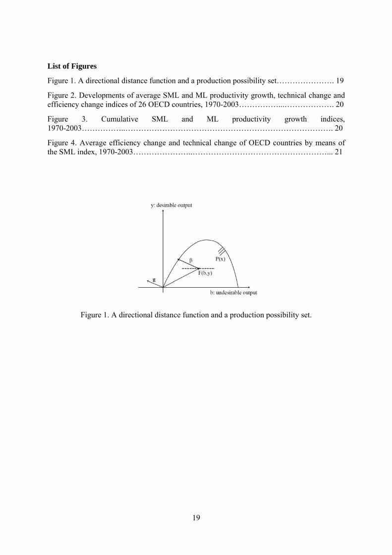
The PPS, which satisfies all the above assumptions, can be depicted in an outputs space, as illustrated in Figure 1. In order to represent it in a simple way, a case with one desirable good and one undesirable good is illustrated in this figure. In depicting the PPS, without loss of generality, it is assumed that the producers use the same amount of input. The horizontal axis represents the undesirable good, and the vertical axis represents the desirable good. All producers are producing combinations of the desirable and undesirable outputs in the inner area of the solid curve. Producers on the solid curve are assumed to be producing on the production frontier. These are utilized as thd

5

2.2. The ML and SML indices

The PPS can be elaborated by employing the directional distance function. Let ( ) y bg g g

be a direction vector, where M JR R g

( )}

. Then, the directional distance function is defined

as follows:

(6) ( ) max{ ( )D y b y bx y b g g y g b g P x

This function seeks the maximum increase of the desirable outputs while simultaneously reducing the undesirable outputs. The direction vector, g , determines the direction of outputs, by which the desirable outputs increase and the undesirable outputs decrease. The process of determining the direction vector is dependent on the purpose of study and policy implications. For example, Arcelus and Arcena (2005) apply three types of direction vectors in analyzing the environmentally sensitive efficiency of OECD countries. They examine the effects of environmental regulations which are assumed to be represented by the direction vectors. Since the purpose of this study is not to show the effect of selecting direction vectors when measuring the environmentally sensitive productivity growth, the direction vector is chosen following the pioneering work of Chung et al. (1997). Hence, in the present study, the direction vector was taken as ( )g y b .

Looking at Figure 1 again, the direction vector and the directional distance function are depicted for a DMU F. Again, the PPS is represented by the inner area of the solid curve. The direction of the directional distance function of the DMU F is depicted as an arrow from the origin towards northwest direction.1 Hence, the directional distance function of the DMU is represented as in Figure 1.

Since the ML index and SML index require a heavy dose of additional notations, we shall omit the direction vector ( )g y b when defining and calculating the indices in the

remainder of this paper. For example, in all places we replace ( )D x y b y b

with

( )D x y b

.

To define and decompose the SML index, two definitions of the PPS are essential for the calculation of the distance functions: a contemporaneous PPS and a sequential PPS. The contemporaneous PPS at time period t is defined as

( ) {( ) can produce ( )}t t t t t t t| P x y b x y b with 1t T . It constructs a reference production set at each point in time , made from the observations at that time only. The sequential PPS at time period is defined as

tt 1 1 2 2( ) ( ) ( ) ( )t tt x P x P x P xP t

, where . It establishes a reference production set using the observations from the point in

time 1 up to time t. The definition of the sequential PPS defined above may look similar to that of Tulkens and Vanden Eeckaut (1995). However, the two definitions are quite different in the sense that our definition includes the desirable and undesirable outputs, whereas their definition only includes the desirable outputs. Also note that the definition of the sequential PPS is the superset of a single contemporaneous PPS. This favorable feature of the sequential PPS enables us to redefine the environmentally sensitive productivity growth index considering the features of technology.

1 t T

1 The direction is determined by the production point of the DMU under our consideration.

6

By using the definition of the contemporaneous PPS, a contemporaneous ML index (equivalently, the conventional ML index) between time period and is defined as follows (Chung et al. 1997):

t 1t

(7) 1 1 1

(1 ( ))

(1 ( ))

s t t ts c

s t t tc

DMLD

x y b

x y b

where the contemporaneous directional distance functions, , are defined on each of the

contemporaneous PPS at the time period . The subscription “ ” in the directional distance function represents the “contemporaneous”. In order to avoid choosing an arbitrary benchmark technology, a geometric mean form of two adjacent contemporaneous ML productivity indices is typically used, expressed as

( ) max{ ( ) ( )}s sc s t tD x y b y y b b P x

s

ML

1

1 1 2]

c

1 ML[t t t tML . The ML index can be decomposed into the efficiency change and technical change. The decomposition is discussed in details in Chung et al. (1997). We omit the further discussion of this issue in order to save space.

In a similar way, the SML index between time period t and 1t is defined on the sequential PPS, ( )ss xP , as follows:

(8) 1 1 1

(1 ( ))

(1 ( ))

s t t tqs

s t t tq

DSMLD

x y b

x y b

where the sequential directional distance functions, ( ) max{ ( ) ( )}s s

q s t tD x y b y y b b xP 1

t

, are defined on each of the

sequential PPS. The subscription “ ” of the sequential distance function represents the

“sequential” nature of the index. Since in general

q1tSML SML without any restrictions on

two production technologies, we also use a geometric mean form of these two SML productivity indices to avoid choosing an arbitrary benchmark technology. The SML index as a result is redefined as:

(9)

1 211

11 1 1 1 1 1

(1 ( )) (1 ( ))

(1 ( )) (1 ( ))

t tt t t t t tq qt t

t tt t t t t tq q

D DSMLD D

x y b x y b

x y b x y b

Obviously, if the contemporaneous PPS at is contained in the contemporaneous PPS at +1 for all , then the SML productivity index is equivalent to the

contemporaneous ML index.

ss )

)

( 1s T

If for all , then 1 1( ) ( )s s s s P x P x ( 1s T 1 1s s sSML ML s

)

.

Proof. for all 1 1( ) ( )s s s s P x P x ( 1s T implies that 1 1 2( ) ( )2( ) ( )s s sP x P P xs x P x , which results in ( ) ( )s s ss x P xP . Then

( ) ( )s ss s s x y b s s sq cD D x y b

since

max ( ) ( )s s s s ss{ } max ( s s s{ ) ( )s s s }y y b b x y y b b P xP1 11 1 1 1 1( ) ( )s ss s s s s s

q cD D x y b x y b

. Also,

. 1

7

This also implies that 1 1( ) (s s )s s s s s sq cD D x y b x y b

since

1 1( ) (s s s s s{ y y b b P1 1( )s

11max ( ) ( ) max )s s s s s ss{ } } y y b b x xP

. It is

trivial to show . 1 1 1 1( )s ss s s s sq cD D

x y b x y b

Hence, 1 1s s sSML ML s .� �

Note that the converse of Proposition 9 is not true.

2.3. Decomposition of the SML index

The geometric mean form of the SML productivity index can be decomposed into two main components as follows:

(10)

11 1 1 1

1 21 1 1 1 1

1 1 1

1 1

1 ( )

1 ( )

1 ( ) 1 ( )

1 ( ) 1 ( )

t t t tqt t

t t t tq

t tt t t t t tq q

t tt t t t t tq q

t t t t

DSMLD

D D

D D

EC TC

x y b

x y b

x y b x y b

x y b x y b

where efficiency change component, 1t tEC

t, represents a movement of a DMU towards the

best practice frontier from time period to 1t ; the technical change, , measures amount of a shift of frontier between t and

1t tTC

1t . The 1t tEC

1t tSML

component measures a catching-up effect and an innovative effect of the DMU. If there have been no changes in inputs and outputs over two time periods, then

1t tTC

1 . If there has been an increase (decrease) in productivity then . It should be noted that the above discussion assumes an unchanged relationship between the two types of outputs.

1t t ( ) 1SML

Changes in efficiency are captured by 1t tEC , which gives a ratio of the distances the DMU are to their respective frontiers in between the time periods and t 1t . If , then there has been a catching up movement or convergence towards the frontier in period

1 1t tEC t 1 . It

is interpreted as an improvement in efficiency. If 1 1t tEC , then it indicates that the country is further away or diverging from the frontier in 1t compared to , and hence it has become less efficient.

t

The technical change component is captured by 1t tTC . The 1t tTC measures the amount of a shift of the frontier between two time periods and t 1t . Note that the technical change index in the SML index is always larger than unity since

. If technical change enables more production of

desirable outputs and less production of undesirable outputs, then , otherwise . It should be noted that the technical change component in the ML index can be

less than unity, indicating technical regress.

1( ) ( )t ts s s s s sq q s t tD D x y b x y b

1 1t tTC

1

1 1t tTC

8

2.4. Calculation of directional distance function

The directional distance function can be calculated in several ways. Färe et al. (2006) and Färe et al. (2005) specify the directional distance function as a quadratic form and employ a linear programming (LP) approach. Other studies by Färe et al. (2007), Kumar (2006), Lee et al. (2002) and Chung et al. (1997) employ a data envelopment analysis (DEA)-type linear programming approach. The above two estimation methods are very similar in that they employ a linear programming in the calculation process. However, two main differences between the two methods can be distinguished: (i) the former approach has an advantage that it can easily calculate the shadow prices, whereas it requires an assumption of the functional form of the directional distance function and imposes lots of restrictions on parameters, and (ii) even though the latter approach does not directly yield the shadow prices, it has advantages in that it requires neither any functional form of the directional distance function nor any restrictions to be imposed on the parameters.2 Since the calculation of the shadow price is not within our research scope in the present study, we employed the latter approach. By choosing this approach, we can secure necessary flexibilities in the estimation process. The methodological aspect of the chosen DEA-type approach will be discussed in calculating the directional distance functions of the SML index.

Let us assume that there are DMUs of inputs and outputs 1k K ( )k k k x y b for time

period 1 T . Using this data, the sequential production technology frontier can be established in the DEA framework as follows:

(11)

1

1

1

( ) {( )

0}

ss

s

s

|

x y b Y z yP

B z b

X z x

z

where Y is a ( )M K matrix of desirable outputs, B is a matrix of

undesirable outputs, and

(J K )X is a (N K ) matrix of inputs for time period , respectively;

y , and are a vector of desirable outputs, a b x 1) )(M (J 1 vector of undesirable

outputs, and a vector of inputs, respectively; (N 1) z is ( 1)K column vector which represents intensities assigned to each observation in constructing the sequential production possibility frontier.

In order to calculate and decompose the SML productivity index of country between time period and , we need to solve four different LP problems. Two of them utilize the same time period for observations and a sequential PPS, while the remaining two utilize the mixed time period for observations and a sequential PPS:

kt 1t

( )t t t tqD x y b

, , 1tq 1 1 1( )t t t

D x y b

1 1t t tqD

x 1( )t y b

) and 1(t t t tqD x y b

. By using the empirical PPS shown in equation (11),

2 The shadow price can be obtained if a dual linear programming is employed.

9

the first sequential directional distance function of the country , k )(t t t tqD x y b

, can be

calculated by solving the following LP problem:

(12)

1

1

1

( ) max

s t (1 )

(1 )

0

t t t tq k k k

ttk

ttk

ttk

D

x y b

Y z y

B z b

X z x

z

The computation of 1 1 1 1(t t t tqD x y b )

is almost the same as equation (12), except that the

superscript is substituted for superscript of variables on the right hand side of the constraint.

1t t

The remaining two distance functions used in construction of the SML productivity index require mixed-period information. The first of these, 1 1(t t t

qD1)t x y b

, is computed for the

country as: k

(13)

1 1 1

1

1

1

1

1

1

( ) max

s t (1 )

(1 )

0

t t t tq k k k

ttk

ttk

ttk

D

x y b

Y z y

B z b

X z x

z

1 1t tk k x 1( )t

kyIn equation (13), the reference technology which is evaluated at by b is

constructed from all observations over the period from 1 to . The last LP problem we need to solve,

t1(t t t t

qD x ) y b

t

, is also a mixed-period problem. It is specified as in equation (13),

but the superscript and are transposed. 1t

Optimal solutions in equation (12), equation (13) and their modified versions are employed in calculating and decomposing the SML index.

3. Empirical Study

As part of the empirical study, the data is described and the two productivity indices, ML and SML, are computed for each of the sample countries and periods. In analyzing the results, the focus is on comparison of the productivity indices, country heterogeneity and their innovativeness.

10

3.1. Description of the data

ely, GDP, , labor force, capital stock, and

obtained by merging the Penn World Table

of le 2. The

As regards emissions, the an our sample is around 1.68%. The

rowth

We obtained the data on five variables nam 2CO

commercial energy consumption for 26 OECD countries over the periods 1970–2003 from Penn World Tables and World Development Indicators. The Czech Republic and Slovakia are excluded from the empirical analysis since these two countries lack data for the period 1970-1995; Hungary and Poland were also excluded from the analysis due to the unavailability of capital stock information over the study period. Among the first two variables, GDP is chosen as a proxy of the desirable output, and 2CO is a proxy of the

undesirable output. Labor force, capital stock, and commercial energy consumption are chosen as the inputs of production technology.

Data on GDP, labor force, and capital stock are(Mark 5.6) and the Penn World Table (Mark 6.2). Since the capital stock for the period 1990–2003 is not available for all countries, we estimated capital stock using the investment series contained in the Penn World Table (Mark 6.2). The capital stock series is created using the capital stock definition stated in the Penn World Table (Mark 5.6) and gross investment information in the Penn World Table (Mark 6.2). We employed the perpetual inventory method for this purpose. In doing so, we assumed that the depreciation rate is 10% per year. GDP and capital stock are transformed and are measured in 2000 US dollars. Data on 2CO

emissions per capita and energy consumption per capita are taken from the website of World Development Indicators. These are multiplied by each national population in order to get the total emissions of 2CO and the total consumption of energy at the country level.

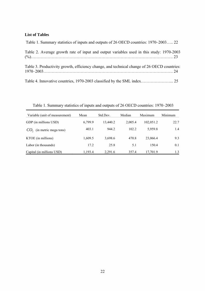
Summary statistics variables used in this study are shown in Table 1 and Tabaverage growth rate of GDP of our sample is 3.02% per year. The highest growth rate with respect to GDP was observed in the Republic of Korea (6.97%), followed by Ireland (4.84%), Luxembourg (4.13%) and Turkey (3.93%). Switzerland (1.42%), Sweden (1.88%) and Denmark (1.88%) show the slowest GDP growth rate during the study period.

[Table 1 about here]

2CO nual growth rate of

Republic of Korea, recorded as the fastest growing economy, is found to be the highest 2CO

emitter (6.57%). This figure is around four times as much as the mean rate of our sam Turkey (5.01%), Portugal (4.34%), Mexico (4.24%) and Greece (4.18%) are also found to be major emitters. Interestingly around one quarter of our sample had a negative growth rate of

2CO emissions. Those countries are Sweden (-1.71%), Luxembourg (-0.97%), Germany

9%), Belgium (-0.62%), France (-0.41%), Denmark (-0.39%) and UK (-0.30%).

The average growth rate of energy usage of our sample is around 2.36%. The average g

ple.

(-0.6

rate of energy usage of the Republic of Korea is also registered as the highest (8.15%). Turkey (4.44%), Portugal (4.44%), Mexico (4.42%) and Greece (3.96%) are registered as countries having relatively high growth rates of energy usage. Denmark (0.08%), Luxembourg (0.08%), UK (0.35%), Germany (0.40%) and Sweden (0.90%) recorded very low growth rates in energy usage. An examination of the growth rates of 2CO emissions and

11

energy usage leads us to conjecture that countries having a high (low) growth rate of 2CO

emissions are also registered as those having high (low) growth rate of energy usage. correlation between 2CO emissions and energy usage is quite high (0.998), which signifies

that a high growth rate of energy usage has induced a high growth rate of 2CO emissions as

argued by Ramanathan (2005). The average growth rates of labor and capital stock of our sample are around 1.24% and 5.46%.

[Ta

The

easures

e SML

ble 2 about here]

.2. A Comparis the ML and SML indices

The approach described in the methodology section constructs the best-practice sequential

As can be seen in panel (a) of Figure

development of technical change m by th

educed from panel (b) of Figure 2 is that the technical change

3 on of

fact d

technology frontier from the data. First, we report the average productivity growth and its decomposed components including efficiency change and technical change calculated by the two methodologies. These are shown in Figure 2. The rates of productivity growth, efficiency change and technical change are shown in the upper panel, middle panel and lower panel of Figure 2, respectively. In this figure, solid lines and dotted lines are productivity (component) indices calculated from the SML index and ML index, respectively.

[Figure 2 about here]

2, the rates of productivity growth of the two m

easured

show very similar trends, signifying that the productivity measures calculated by the two methodologies are similar. The correlation coefficient between the SML and the ML indices is quite high, 0.881. We also tested the null hypothesis that the two productivity growth measures have the same rank by using the Wilcoxon rank sum test. We failed to reject the null at the 1% level of significance, indicating that the ranks of the two productivity growth measures can be regarded as being identical. Based on those two test statistics, it is inferred that the productivity growth indices computed based on the two methodologies in aggregate form are not statistically different.

A priori, one would expect that the framework is different from that of the ML framework, which is confirmed by the trends of technical changes shown in panel (b) of Figure 2. In the technical change measure of the ML index, a total of fifteen years of technical deterioration is observed. Especially during 1970-1981 the technology is recorded as being regressed. However, as discussed in the introduction section, this technical change measure is considered as being biased since such a long-run technical regress is not possible from the macroeconomics perspective. In the technical change of the SML index, on the other hand, the rate of technical change is larger than or equal to unity for all periods. Trends of technical change components of the two methodologies are different when the rate of technical change of the ML index is less than unity, but they show a similar pattern when the ML index is larger than unity. We can observe this similarity in particular at the end of the sample period. This appears to indicate that innovatory technology related to energy and carbon dioxide emissions has emerged during this period.

Another interesting measure of the ML index shows much more volatility than the sequential one. This is because

12

it classifies each change in productivity of countries that belong to the frontier as technical change. On the contrary, the technical change measure in the SML index registers only those changes that lead to the expansion of the PPS. Those differences can be found around the two oil crises of 1973 and of 1979. These oil crises caused lagged overall fall in productivity. It appears that these oil crises affect the declines in the technical change measure of the ML index, whereas they have no impact on that of the SML index.

Compared to the similarity in the patterns of productivity growth between the two

up the world frontier when the above two conditions are

iciency change measure of the ML index, that of the SML index is free

methodologies, the development of efficiency of the SML index is very different from that of the ML index. Not only the correlation coefficient is negative (-0.493), but also the Wilcoxon rank sum test statistics is not statistically significant (p-value is 0.929), indicating inconsistency between the two indices. This dissimilarity in the efficiency change needs to be investigated through the simultaneous examination of the behavior of the PPS and our assumptions imposed when constructing the PPS. Before discussing this dissimilarity, it should be noted again that the efficiency change captures the speed at which a country moves towards the world technology frontier. As already discussed earlier, this measures a catching-up effect. It is obvious that the efficiency gain occurs if the PPS does not change and an input/output bundle of a country moves closer towards the world technology frontier. Even when the PPS expands, the efficiency gain can occur if the convergence speed is faster than the speed of PPS expansion.

It is obvious that a country catchessatisfied. If the PPS contracts, however, a very different story unfolds. That is, the efficiency of a country increases even when it does not attempt to squeeze its endowed inputs to catch up the world frontier technology only if the PPS contradicts. In this case the country’s distance from the world technology frontier is automatically shortened by the contraction of the PPS. This counterfeit catching-up effect can be seen as merely the resultant effect of a free lunch which is prepared by the temporary technological deterioration of the world frontier countries. In other words, the country, although it does not do anything, is recorded as having caught up the world frontier technology if we allow the temporal contraction of the PPS. This is one of drawbacks of the ML index. As a result of the efficiency change component of the ML index, especially during the period 1970-1980, this counterfeit catching-up effect is observed many times. Considering that during the same period the technology is spuriously measured as being deteriorated for a long time period, this counterfeit catching-up originates from the assumption imposed when constructing the PPS of the ML index.

Contrary to the efffrom this counterfeit catching-up effect problem. Because the temporal contraction of the PPS is absorbed by the previous PPS under the framework of the SML index, the abnormal catching-up cannot occur. In this sense, the catching up effect measured by the SML index can be seen as being the genuine catching-up effect compared to that of the ML index.

The two components of the productivity growth measure, i e , efficiency change and technical change, contribute to the development of productivity. In many previous studies such as Chung et al. (1997), Yörük and Zaim (2005) and Kumar (2006), it is reported that productivity growth is mainly attributed to technical change rather than efficiency change. This is true if we only look at the result of the ML index as investigated in the previous studies. That is, the trend of productivity growth is quite similar to that of technical change under the framework of the ML index, as can be seen in the panel (a) and (b) of Figure 2. The correlation coefficient between the ML productivity growth index and the technical change

13

index of the ML index is 0.958, while the one between the ML productivity growth and the efficiency change of the ML index is -0.526. This supports the argument under the framework of the ML index approach.

Looking at the result of the SML index, however, it is easily induced that this argument is not

The cumulative productivity growth measure is also economically meaningful since it gives

Average productivity growth, efficiency change and technical change are calculated for the

[Table 3 about here]

always true. In earlier years of the study period, where the technology rarely changes, the productivity growth is mainly attributed to efficiency change. Nonetheless, the influence of technical change becomes more attributable to the productivity growth over time. This increasing influential pattern of technical change appears to reflect recent technological development related to energy and environment. The recent increasing frequency of policies and protocols launched related to energy and the environment, such as the sustainable growth policies, may be attributed to this trend.

[Figure 3 about here]

us information about how much productivity is accumulated over time. The cumulative productivities of our sample using the two productivity indices are depicted in Figure 3. In this figure, the productivity growth of the first year is adjusted to unity so that the developments of the two measures are easily compared. Even though temporal developments of productivity growth measured by the two methodologies are similar to each other, as discussed earlier, their cumulative versions are apparently different in two ways. First, the productivity measures diverge over time. The cumulative productivity growth for the study period measured by the SML index is 18.1%, and the one measured by the ML index is -8.4%. Second, the cumulative productivity of the SML index becomes larger than unity from 1986, whereas that of the ML index is less than unity for whole study period. Reconsidering the recently increasing concerns and policies about energy and the environment, the positively cumulated productivity growth of the SML index appears to reflect recent changes better than that of the ML index.

3.3. Country Heterogeneity

sample countries. These measures are listed in Table 3. Recall that index values greater (less) than unity indicate improvement (deterioration) in the relevant performance. As expected from the result of the temporal development of productivity growth and its decomposed sources discussed in the previous subsection, the two methodologies yield different measures and decompositions. The number of countries having productivity deterioration is seven in the SML index, while the corresponding number in the ML index is twenty. This large discrepancy between the two methodologies is caused by the different assumption imposed in constructing the PPS. Looking at the decomposed sources of productivity in the two methodologies, the differences are more profound compared with the aggregate level. Regardless of selection of the methodology, Australia, Finland, Italy, Luxembourg, Norway, Switzerland and the USA have positive rate of productivity growth; while Greece, Iceland, Mexico, New Zealand, Portugal, Spain and Turkey show a negative productivity growth for both measures.

14

In order to examine the relationship among the three performance (efficiency change, technical change and productivity growth) measures, a scatter plot is depicted with x-axis of an efficiency change index and y-axis of a technical change index, as shown in Figure 4. The size of the circle in this figure gives us information about the average annual growth rate of productivity.

[Figure 4 about here]

Our sample countries can be classified into several groups in accordance with the following categorization rule. The countries are categorized into a specific group based on their performance in the rates of technical change and efficiency change. If the technical change index of a country is larger (smaller) than the average technical change of our sample, its innovative ability can be considered as being better (worse) than the virtual average country. Likewise, if the efficiency change index of a country is larger (lesser) than unity, it is considered as being in the state of catching up (lagging behind) the world frontier technology, as discussed in the methodology section. Hence, in the present study the criterion of our categorization is set as the average technical change of our sample and a unit efficiency change. Through this categorization rule, we can divide the OECD member states into four groups: more innovative and catching-up countries (Group I), more innovative but lagged countries (Group II), less innovative but catching-up countries (Group III) and less innovative and lagged countries (Group IV).

In Figure 4, those country groups are placed in the northeast, northwest, southeast and southwest spaces. Belgium, Luxembourg and Norway are categorized as Group I countries; Australia, Canada, Switzerland and the USA are categorized as Group II; Finland, France, Ireland, Italy, Korea and Sweden are categorized as Group III countries; and finally Austria, Denmark, Germany, Greece, Iceland, Japan, Mexico, New Zealand, Portugal, Spain, Turkey and UK are categorized as Group IV countries. In the Group IV, it is worth noting that more than half the countries have negative productivity growth. Another interesting fact deduced from Figure 4 is that, except for Iceland, the Nordic countries are categorized as high productivity growth countries. For example, Norway is good at innovating as well as catching up the world frontier technology; Finland and Sweden are also good at catching up the world frontier technology. This favorable state of the Nordic countries can be considered as a benchmark for a successful sustainable economic growth policy.

3.4. Innovative countries

The technical change index for any one particular country between two adjacent years, if not on the frontier, is not necessarily an index of the shift in the world technology frontier. Hence, a value of this factor greater than unity does not necessarily imply that the country under consideration actually pushes the world technology frontier outwards. This means that additional information needs to be investigated in order to determine which countries are the world innovators. The following three conditions help us determine this issue:

(13.a) 1 1t tTC

(13.b) 1 1 1( )t t t tqD

x y b

0

15

(13.c) 1 1 1 1( )t t t t

qD x y b

0

t

t

As discussed earlier, the first condition indicates that the world technology frontier is shifted in more good outputs and fewer bad outputs direction. This means that in period it is possible to increase GDP and to decrease the level of emissions relative to period .

This measures the shift in the relevant portions of the frontier between period and t

1t 2CO

1 for a given country when the good and bad outputs are treated asymmetrically. The second condition indicates that production in period 1t occurs outside the PPS of period . This means that technical change has occurred during the transition period. It implies that technology of period t cannot produce the output vector of period with the input vector of period . Hence, the value of the directional distance function evaluating input/output vector at period relative to the reference technology of period is less than zero. The third condition indicates that the country should be on the world technology frontier in period . In should be noted that, since our sample countries contain all advanced countries, we are confident that the estimated frontier represents the world frontier technology.

t

t

1t 1t

t

1t

1

Table 4 lists the innovative countries for every five-year period from 1970 to 2003. Out of 26 OECD countries, nine countries are recorded as the innovative countries. Those countries are Austria, France, Italy, Luxembourg, Norway, Portugal, Sweden, Switzerland, and the USA. Some countries are innovators only for a short period, e.g., Portugal and the USA, whereas others are innovators covering almost the entire study period, e.g., Luxembourg and Switzerland. As expected, low emitters coupled with high GDP growth, such as

Luxembourg and Switzerland, are recorded as innovative countries. High emitting

countries, such as Korea and Turkey, are not found to be innovators in spite of the fact that their rate of GDP growth is quite high. Interestingly, only two of the Nordic countries (Norway and Sweden), which are among high productive economies, are recorded as the innovators during the period 1990-2000. Although not all of them are the innovators, the Nordic countries appear to be good at following the world frontier technology closely and are only slightly lagged by the top innovators.

2CO

2CO

[Table 4 about here]

4. Conclusion

Although productivity is not the only determinant of economic growth and welfare, it does provide an indirect measure of the economic prosperity, as well as of the standard of living and of the degree of competitiveness of a country. As the environmental concern has remarkably grown during recent decades, the classical productivity growth indices such as the Malmquist productivity index have attempted to integrate the effect of environmentally harmful by-products. Those attempts have resulted in the creation of the environmentally sensitive productivity index by expanding the classical productivity index, such as the Malmquist-Luenberger index. Although this productivity measure considers the environmental and economic perspectives of the relationship between the desirable and undesirable outputs, it fails to appropriately integrate the features of technology.

In order to overcome this weakness of the conventional ML index, we developed an alternative environmentally sensitive productivity growth index. It was done by combining the two concepts of the directional distance function and the successive sequential reference

16

production set. We named it the sequential Malmquist-Luenberger productivity index (SML index). With this augmented methodology, the components of the productivity growth, such as the efficiency change and technical change indices, are properly measured without bias by eliminating the possibility of the contraction of the production possibility set.

The proposed methodology was employed in measuring the environmentally sensitive productivity growth of 26 OECD countries over the period 1970–2003. The empirical results show that: (i) although the developments of the productivity calculated by the ML and SML index are similar to each other, the components of the productivity indices are quite different, (ii) unlike the previous studies, the efficiency change is found to be the main contributor of the productivity growth in the earlier study period, whereas the effect of technical change prevails over time, (iii) by categorizing OECD countries, Belgium, Ireland, Luxembourg and Norway are found to be good at innovating as well as catching up the world frontier technology, (iv) Luxembourg and Switzerland are found to be innovative countries for most of the study period, and (v) the environmentally sensitive productivity growth of the Nordic countries are on average higher than that of the rest of the OECD member states.

Beyond presenting an alternative measure, the present paper is believed to pave th

e way for further methodological development related to the needy environmentally sensitive productivity growth measure. A combination of the concept of the metafrontier (Hayami 1969) and the directional distance function would be a good nominee of those methodological developments in order to facilitate the investigation of group heterogeneity among the sub-samples. We believe that this study will be a roadmap for opening up the possibility of expanding the existing environmentally sensitive productivity growth index. We also believe that the results of the empirical study will have implications for policy-making related to sustainable growth.

17

References Arcelus FJ, Arocena P (2005) Productivity differences across OECD countries in the presence of environmental constraints. J Oper Res Society, 56(12):1352–1362.

Chung YH, Färe R, Grosskopf S (1997) Productivity and undesirable outputs: A directional distance function approach. J Environ Manage, 51(3):229–240.

Färe R, Grosskopf S, Noh DW, Weber W (2005) Characteristics of a polluting technology: Theory and practice. J Econometrics, 126(2):469–492.

Färe R, Grosskopf S, Pasurka CA Jr (2001) Accounting for air pollution emissions in measures of state manufacturing productivity growth. J Reg Sci, 41(3):381–409.

Färe R, Grosskopf S, Pasurka CA Jr (2007) Environmental production functions and environmental directional distance functions. Energy, 32(7):1055–1066.

Färe R, Grosskopf S, Weber WL (2006) Shadow prices and pollution costs in U.S. agriculture. Ecolog Econ, 56(1):89–103.

Hayami Y (1969) Sources of agricultural productivity gap among selected countries. Amer J Agr Econ, 51:564–575.

Kumar S (2006) Environmentally sensitive productivity growth: a global analysis using Malmquist-Luenberger index. Ecolog Econ, 56(2):280–293.

Lee JD, Park JB, Kim TY (2002) Estimation of the shadow prices of pollutants with production/environment inefficiency taken into account: A nonparametric directional distance function approach. J Environ Manage, 64(4):365–375.

Luenberger DG (1992) Benefit functions and duality. J Math Econ, 21(5):461–481.

Nakano M, Managi S (2008) Regulatory reforms and productivity: An empirical analysis of the japanese electricity industry. Energy Pol, 36(1):201–209.

Pasurka CA Jr (2006) Decomposing electric power plant emissions within a joint production framework. Energy Econ, 28(1):26–43.

Ramanathan R (2005) An analysis of energy consumption and carbon dioxide emissions in countries of the middle east and north africa. Energy, 30(15):2831 – 2842.

Shestalova V (2003) Sequential Malmquist indices of productivity growth: An application to OECD industrial activities. J Productiv Anal, 19(2):211–226.

Tulkens H, Vanden Eeckaut P (1995) Non-parametric efficiency, progress and regress measures for panel data: Methodological aspects. Eur J Oper Res, 80(3):474–499.

Weber W, Domazlicky B (2001) Productivity growth and pollution in state manufacturing. Rev Econ Statist, 83(1):195–199.

Yörük BK, Zaim O (2005) Productivity growth in OECD countries: A comparison with malmquist indices. J Compar Econ, 33(2):401–420.

18

List of Figures

Figure 1. A directional distance function and a production possibility set…………………. 19

Figure 2. Developments of average SML and ML productivity growth, technical change and efficiency change indices of 26 OECD countries, 1970-2003……………...………………. 20

Figure 3. Cumulative SML and ML productivity growth indices, 1970-2003……………..……………………………………………………………………. 20

Figure 4. Average efficiency change and technical change of OECD countries by means of the SML index, 1970-2003…………………..……………………………………………... 21

Figure 1. A directional distance function and a production possibility set.

19

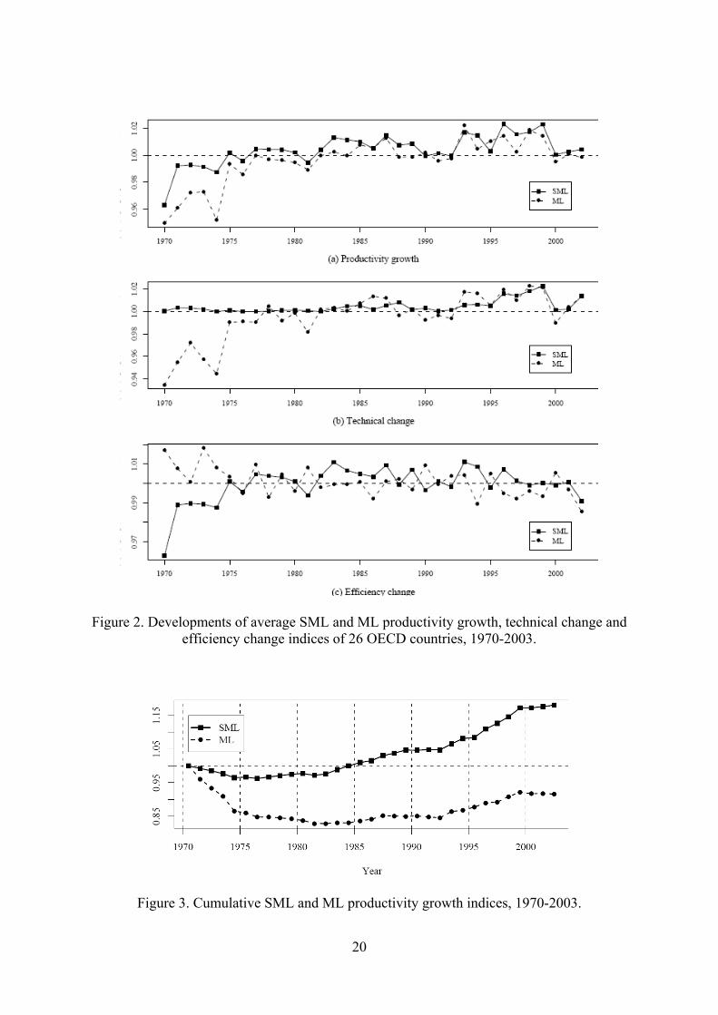
Figure 2. Developments of average SML and ML productivity growth, technical change and efficiency change indices of 26 OECD countries, 1970-2003.

Figure 3. Cumulative SML and ML productivity growth indices, 1970-2003.

20

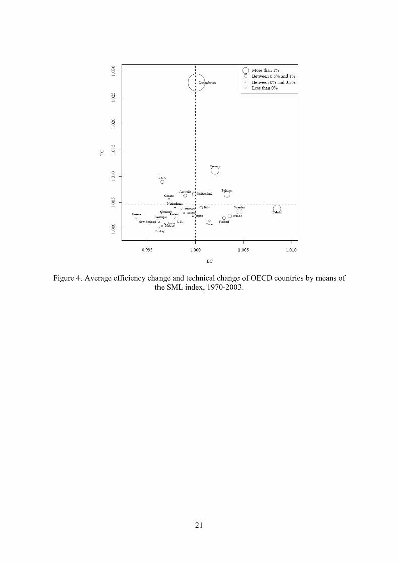
Figure 4. Average efficiency change and technical change of OECD countries by means of the SML index, 1970-2003.

21

List of Tables

Table 1. Summary statistics of inputs and outputs of 26 OECD countries: 1970–2003….. 22

Table 2. Average growth rate of input and output variables used in this study: 1970-2003 (%)…………………………………………………………………………………………. 23

Table 3. Productivity growth, efficiency change, and technical change of 26 OECD countries: 1970–2003…………………………………………………………………………………. 24

Table 4. Innovative countries, 1970-2003 classified by the SML index…………………... 25

Table 1. Summary statistics of inputs and outputs of 26 OECD countries: 1970–2003

Variable (unit of measurement) Mean Std.Dev. Median Maximum Minimum

GDP (in millions USD) 6,799.9 13,440.2 2,005.4 102,051.2 22.7

2CO (in metric mega tons) 403.1 944.2 102.2 5,959.8 1.4

KTOE (in millions) 1,609.5 3,698.6 470.8 23,066.4 9.3

Labor (in thousands) 17.2 25.8 5.1 150.4 0.1

Capital (in millions USD) 1,193.4 2,291.6 357.4 17,701.9 1.3

22

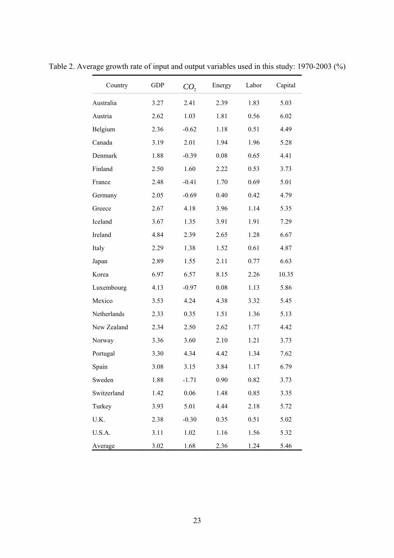
Table 2. Average growth rate of input and output variables used in this study: 1970-2003 (%)

Country GDP 2CO Energy Labor Capital

Australia 3.27 2.41 2.39 1.83 5.03

Austria 2.62 1.03 1.81 0.56 6.02

Belgium 2.36 -0.62 1.18 0.51 4.49

Canada 3.19 2.01 1.94 1.96 5.28

Denmark 1.88 -0.39 0.08 0.65 4.41

Finland 2.50 1.60 2.22 0.53 3.73

France 2.48 -0.41 1.70 0.69 5.01

Germany 2.05 -0.69 0.40 0.42 4.79

Greece 2.67 4.18 3.96 1.14 5.35

Iceland 3.67 1.35 3.91 1.91 7.29

Ireland 4.84 2.39 2.65 1.28 6.67

Italy 2.29 1.38 1.52 0.61 4.87

Japan 2.89 1.55 2.11 0.77 6.63

Korea 6.97 6.57 8.15 2.26 10.35

Luxembourg 4.13 -0.97 0.08 1.13 5.86

Mexico 3.53 4.24 4.38 3.32 5.45

Netherlands 2.33 0.35 1.51 1.36 5.13

New Zealand 2.34 2.50 2.62 1.77 4.42

Norway 3.36 3.60 2.10 1.21 3.73

Portugal 3.30 4.34 4.42 1.34 7.62

Spain 3.08 3.15 3.84 1.17 6.79

Sweden 1.88 -1.71 0.90 0.82 3.73

Switzerland 1.42 0.06 1.48 0.85 3.35

Turkey 3.93 5.01 4.44 2.18 5.72

U.K. 2.38 -0.30 0.35 0.51 5.02

U.S.A. 3.11 1.02 1.16 1.56 5.32

Average 3.02 1.68 2.36 1.24 5.46

23

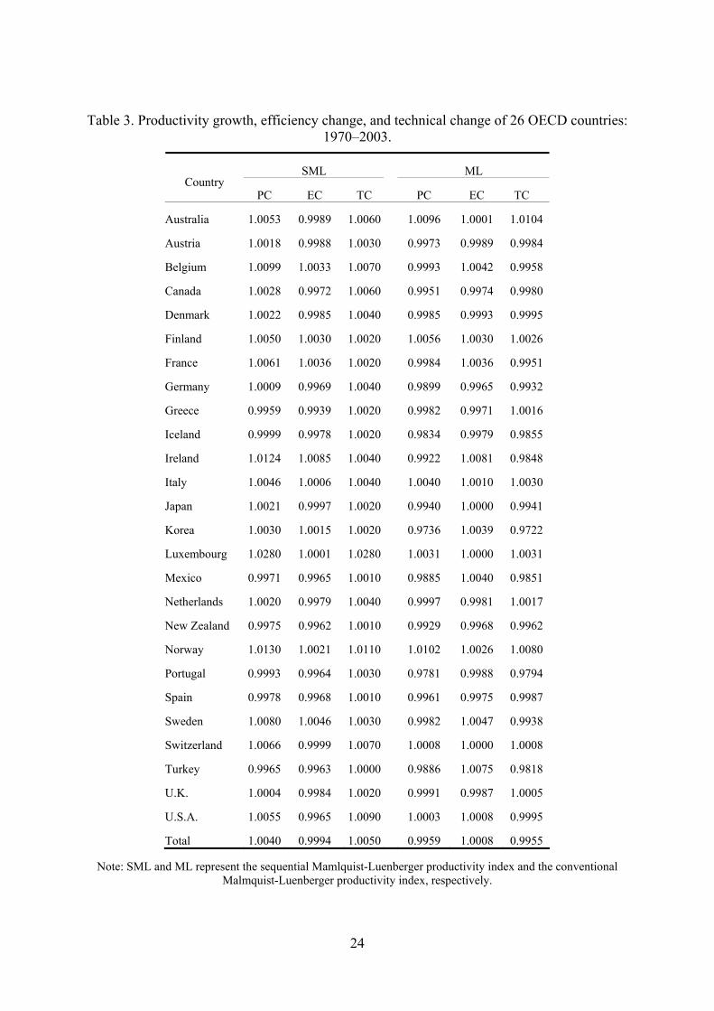
Table 3. Productivity growth, efficiency change, and technical change of 26 OECD countries: 1970–2003.

SML ML Country

PC EC TC PC EC TC

Australia 1.0053 0.9989 1.0060 1.0096 1.0001 1.0104

Austria 1.0018 0.9988 1.0030 0.9973 0.9989 0.9984

Belgium 1.0099 1.0033 1.0070 0.9993 1.0042 0.9958

Canada 1.0028 0.9972 1.0060 0.9951 0.9974 0.9980

Denmark 1.0022 0.9985 1.0040 0.9985 0.9993 0.9995

Finland 1.0050 1.0030 1.0020 1.0056 1.0030 1.0026

France 1.0061 1.0036 1.0020 0.9984 1.0036 0.9951

Germany 1.0009 0.9969 1.0040 0.9899 0.9965 0.9932

Greece 0.9959 0.9939 1.0020 0.9982 0.9971 1.0016

Iceland 0.9999 0.9978 1.0020 0.9834 0.9979 0.9855

Ireland 1.0124 1.0085 1.0040 0.9922 1.0081 0.9848

Italy 1.0046 1.0006 1.0040 1.0040 1.0010 1.0030

Japan 1.0021 0.9997 1.0020 0.9940 1.0000 0.9941

Korea 1.0030 1.0015 1.0020 0.9736 1.0039 0.9722

Luxembourg 1.0280 1.0001 1.0280 1.0031 1.0000 1.0031

Mexico 0.9971 0.9965 1.0010 0.9885 1.0040 0.9851

Netherlands 1.0020 0.9979 1.0040 0.9997 0.9981 1.0017

New Zealand 0.9975 0.9962 1.0010 0.9929 0.9968 0.9962

Norway 1.0130 1.0021 1.0110 1.0102 1.0026 1.0080

Portugal 0.9993 0.9964 1.0030 0.9781 0.9988 0.9794

Spain 0.9978 0.9968 1.0010 0.9961 0.9975 0.9987

Sweden 1.0080 1.0046 1.0030 0.9982 1.0047 0.9938

Switzerland 1.0066 0.9999 1.0070 1.0008 1.0000 1.0008

Turkey 0.9965 0.9963 1.0000 0.9886 1.0075 0.9818

U.K. 1.0004 0.9984 1.0020 0.9991 0.9987 1.0005

U.S.A. 1.0055 0.9965 1.0090 1.0003 1.0008 0.9995

Total 1.0040 0.9994 1.0050 0.9959 1.0008 0.9955

Note: SML and ML represent the sequential Mamlquist-Luenberger productivity index and the conventional Malmquist-Luenberger productivity index, respectively.

24

25

Table 4. Innovative countries, 1970-2003 classified by the SML index. Period List of innovative countries

1970-1975 Luxembourg, Portugal, Switzerland

1975-1980 Switzerland

1980-1985 Luxembourg, Switzerland, USA

1985-1990 Luxembourg, Switzerland

1990-1995 Italy, Luxembourg, Norway, Switzerland

1995-2000 Austria, France, Luxembourg, Norway, Sweden, Switzerland

2000-2003 Austria, France, Italy, Italy, Luxembourg, Sweden, Switzerland