Autonomous Robots (2018) 42:1231–1248https://doi.org/10.1007/s10514-017-9688-z

A sensor-based approach for fault detection and diagnosis for roboticsystems

Eliahu Khalastchi1 ·Meir Kalech1

Received: 11 February 2016 / Accepted: 18 November 2017 / Published online: 7 December 2017© Springer Science+Business Media, LLC, part of Springer Nature 2017

AbstractAs we rely more on robots, thus it becomes important that a continuous successful operation is maintained. Unfortunately,these sophisticated, machines are susceptible to different faults. Some faults might quickly deteriorate into a catastrophe.Thus, it becomes important to apply a fault detection and diagnosis (FDD) mechanism such that faults will be diagnosed intime, allowing a recovery process. Yet, some types of robots require an FDD approach to be accurate, online, quick, ableto detect unknown faults, computationally light, and practical to construct. Having all these features together challengestypical model-based, data-driven, and knowledge-based approaches. In this paper we present the SFDD approach that meetsthese requirements by combining model-based and data-driven techniques. The SFDD utilizes correlation detection, patternrecognition, and a model of structural dependencies. We present two different implementations of the SFDD. In addition,we introduce a new data set, to be used as a public benchmark for FDD, which is challenging due to the contextual natureof injected faults. We show the SFDD implementations are significantly more accurate than three competing approaches, onthe benchmark, a physical robot, and a commercial UAV domains. Finally, we show the contribution of each feature of theSFDD.

Keywords Model-based · Data-driven · Fault detection · Fault diagnosis · Sensors · Robotics

1 Introduction

The use of robots in our daily lives is increasing. Recentreports by the International Federation of Robotics (IFR2016a, b) describe yearly increases of 15% and 25% in salesof service and industrial robots respectively. Robots are usedfor tasks that are too dangerous, too dull, too dirty or toodifficult to be done by humans. Among such tasks we findsurveillance and patrolling (Agmon et al. 2008), aerial search(Goodrich et al. 2008), rescue (Birk and Carpin 2006) andmapping (Thrun 2002).

Robots are complex entities comprising both physical(hardware) and virtual (software) components. They operatein different dynamic physical environments with a varyingdegree of autonomy e.g., satellites, Mars rovers, Unmanned

B Eliahu Khalastchikhalastc@bgu.ac.il

Meir Kalechkalech@bgu.ac.il

1 Information Systems Engineering, Ben-Gurion Universityof the Negev, Beersheba, Israel

Aerial, Ground or Underwater Vehicles (UAV, UGV, UUV),Robotic arm in an assembly line, etc. These sophisticated,and sometimes very expensive machines, are susceptible toa wide range of physical and virtual faults such as wear andtear, noise, or software-control failures (Steinbauer 2013).If not detected in time, a fault can quickly deteriorate intoa catastrophe; endangering the safety of the robot itself orits surroundings (Dhillon 1991). For instance, an undetectedengine fault in aUAV(UnmannedAerialVehicle) can cause itto stall and crash. Thus, robots should be equipped with FaultDetection and Diagnosis (hereinafter FDD)mechanisms thatwill allow recovery processes to take place.

In some aspects, robots are not that different from otherphysical systems in the context of FDD; sensors and actu-ators can be found in non-robotic systems as well. Yet, theautonomy and complex behaviors of robots do yield require-ments that challenge typical FDD approaches—even at thelevel of sensors and actuators FDD.

An autonomous robot may be required to continue oper-ating in the presence of faults. Thus, an FDD mechanismmust be quick enough to allow recovery before a catastro-phe occurs, and online, i.e., detect faults as they occur given

123

1232 Autonomous Robots (2018) 42:1231–1248

the data at hand, rather than after the operation is over whereall the data is available. For instance, in an altitude of X, anengine fault must be detected and diagnosed within Y mil-liseconds, to allow an engine restart.

In addition, an autonomous robot may be independentof remote supporting systems. Thus, FDD is carried out onboard the robot, burdening system resources (CPU, Mem-ory), and thus should be kept computationally-light. Forinstance, a rover on Mars cannot wait 22min for a serveron Earth to communicate the fact that the rover has a criticalfault. Thus, the FDD process should be executed onboard therobot without interfering other mission oriented processes.

Another challenge resides in the fact that an autonomousrobot may not have an external source to compare with itsown perception, e.g. a human operator, radar station, otherrobots. If a fault leads to a wrong perception then the entirebehavior of the robot is compromised. To detect faults, anFDD mechanism must generate an expectation based on noother than the perception of the robot, which in itself mightbe faulty.

Complex behaviors, in particular, interaction with thedynamic and uncertain physical environment, yield two addi-tional requirements fromFDD: the ability to detectunknownfaults, and begin practical to construct. Due to the dynamicand complex nature of a robot’s behavior, one cannot accountfor every possible fault in advance. In addition, approacheswhich rely on a high fidelitymodel of such interactionsmightprove to be impractical.

Unfortunately, traditional model-based, knowledge-base,and data-driven approaches for FDD in the literature arechallenged to meet all of these requirements at once, as weelaborate in the related work section. Basically, somemodelsare hard to construct, unknown faults are hard to extrap-olate with knowledge-based approaches and data-drivenapproaches may not be quick and online.

In this paper, we present a Sensor based approach for FaultDetection and Diagnosis for robotic systems—the SFDD.The approach is designed to meet the FDD requirementsfor robots by combining data-driven and model-based tech-niques. In particular, sensor correlation detection and patternrecognition are used to generate an expectation for faultdetection purposes. The fault detection heuristic and thediagnosis process use a practical model of structural depen-dencies. Multiple faults can be diagnosed. In this workwe present two implementations: the basic SFDD and theextended SFDD which includes additional features that sig-nificantly improve the basic SFDD. These algorithms serveas our main contribution.

Our second contribution lies in the introduction of a newdata set which can be used as a public benchmark to evalu-ate FDD approaches. This data set is very challenging sinceit contains (a) different types of faults, (b) varying faultdurations, (c) concurrent occurrence of double faults, and

(d) contextual faults, i.e., data instances that possess val-ues which are valid under one context but are invalid underanother.

Thiswork is an extensionof our previouswork (Khalastchiet al. 2013) which depicted the basic implementation. In thiswork we expand both the theoretical and empirical parts ofthe research. In particular, in the theoretical aspect we ana-lyze the advantages and drawbacks of the basic SFDD. Thesefindings pave theway for the extendedSFDDimplementationpresented here. We greatly expand the empirical evaluationas well. We empirically show that the SFDD implementa-tions are significantly more accurate than three competingapproaches. For this aim we use the new benchmark, a phys-ical robot, and a commercial UAV. In addition, we showthe contribution of each feature that was added to the basicSFDD, resulting in the extended implementation.

2 Related work

Steinbauer conducted a survey on the nature of faults ofautonomous robots (Steinbauer 2013). The survey partici-pants are developers competing in different leagues of theRobocup competition (Anon 2013). Along with softwarefaults (Steinbauer et al. 2005; Kleiner et al. 2008), the sur-vey concludes that hardware faults such as sensors, actuatorsand platform related faults have a deep negative impact onmission success. In this paper we focus on the detection anddiagnosis of such faults.

To handle such faults, one may apply an FDD approach.Three general approaches are usually used for FDD:Knowledge-Based systems, Model-Based, and Data-Drivenapproaches. Knowledge-Based systems (Akerkar and Sajja2010) typically associates recognized behaviors with prede-fined known faults. Thus, potentially all requirements can bemet apart of the ability to detect unknown faults.

Model-Based approaches (Friedrich et al. 1999; Isermann2005; Travé-Massuyès 2014) on the other hand, are veryequipped to detect unknown faults. Instead of modelingdifferent faults, the expected (normal) behavior of each com-ponent is modeled analytically. During operation, the systemoutput is compared to the output given by the model and ahigh residual indicates a fault. For example, in (Steinbauerand Wotawa 2005) and recently in (Wienke 2016) a modelbased approach is used for detecting failures in the controlsoftware of a robot, including of an unknown type.

Model-Based approaches can meet all requirements but amodel might not be available, or impractical to construct dueto the dynamic context of the environment. Steinbauer andWotawa (2010) the authors emphasize the importance of therobot’s belief management and fault detection with respect tothe real-world dynamic environment. InAkhtar andKuesten-macher (2011) the authors address this challenge by the use

123

Autonomous Robots (2018) 42:1231–1248 1233

of naive physical knowledge. The naive physical knowledgeis represented by the physical properties of objects whichare formalized in a logical framework. Yet, formalizing thephysical laws demands great a priori knowledge about thecontext in which the robot operates (environment and task).

Adiagnosismodel canbe automatically generated (Zamanand Steinbauer 2013; Zaman et al. 2013). The authors utilizethe Robot Operating System (ROS) (Quigley et al. 2009) tomodel communication patterns and functional dependenciesbetween nodes. A node is a process that controls a specificelement of the robot, e.g., a laser range finder or path plan-ning. The model used by our proposed approach is different.First, it is general and not based on ROS, and thus can workon other platforms. Second, our model is structural ratherthan behavioral. Even though it is manually constructed,it is practical to construct since the challenge of describ-ing expected behaviors with respect to the environment isavoided. Another key difference is that our model is used forfault detection and not just for diagnosis.

Data-Driven approaches (Golombek et al. 2011; Hodgeand Austin 2004; Kodratoff and Michalski 2014) are modelfree and have a natural appeal for detecting unknown faults.Data-Driven approaches can be divided to outlier detectionand machine learning approaches. Outlier detection, e.g.,(Pokrajac et al. 2007), uses available data to construct a sta-tistical model and to decide whether or not an outlier is theexpression of a fault (Chandola et al. 2009). Being onlinerestricts the FDD approach from having the complete dataof the entire operation; data is available only up to the cur-rent point in time where it is challenging to differentiate faultexpressions from yet-to-be-seen normal behaviors and thusaccuracy is compromised. Online model creation may pro-duce dynamic models that fit very well to the dynamic natureof the robot. Yet, such approaches face the challenge of pro-ducing the dynamic model within the constraints of time andcomputational-load.

On the other hand, machine learning approaches, e.g.,support vector machines (SVM) (Steinwart and Christmann2008), may involve offline preprocessing that reduces onlinecomputations. An FDD model is learned from offline dataand applied online. Supervised learning approaches relyon data that is already labeled for diagnosed faults (Kha-lastchi et al. 2014). Such data is typically unavailable inthe domain of robots. Some approaches, e.g., (Leeke et al.2011; Christensen et al. 2008), depend on the injection offault expressions to the training data prior to the learning.Such approaches face the challenge of mimicking the faultspropagation through the system to correctly inject the fault’sexpressions in the data.

Another possibility is to use unsupervised or one-classclassification techniques. Hornung et al. (2014) utilize adata set of a fault-free operation. They apply two cluster-ing techniques to produce a two-classed labeled data. First,

Mahalanobis-Distance (Mahalanobis 1936) is utilized tocluster data instances depicting normal behavior. Then, neg-ative selection is used to cluster the unknown data instances,i.e., an infinite amount of possible data instances that do notappear in the data and depict the abnormal behavior of therobot. Having the two labels, an SVM learning algorithmis applied offline, and used online as an anomaly detector.For efficiency the high dimension of the data is reduced bytechniques of projection and re-projection. In this paper wecompare our approach to an algorithm based on Hornung etal’s algorithm.

For both supervised and unsupervised approaches it is achallenging task to select general features such that overfit-ting is avoided, and thus the learned model is general enoughto handle previously unobserved behaviors. In addition, theoffline produced model is static. It is challenging to capturethe online dynamic behavior of the robot with static models.In this paper we describe and analyze two implementationsof the SFDD: the basic implementation creates the modelonline, and the extended implementation creates the modeloffline.

Our arguments regarding knowledge-based,model-based,and data-driven approaches are consistentwith the argumentsof Pettersson (2005) which presents a survey about executionmonitoring in robotics. His survey particularly focuses onmobile robots. There is a very good discussion about theadvantages anddisadvantages of each approach.Our researchis focused on hybrid FDD approaches that by combiningmodel-based and data-driven techniques we can avoid thesedisadvantages when applied for robotic systems.

The proposed approach in this paper has evolved from dif-ferent insights learned from previous works. Lin et al. (2010)we showed that dependent data streams, learned offline, formthe clusters needed by outlier detection. Khalastchi et al.(2011, 2015) two interesting insights are shown: (a) linearcorrelation detection is good enough to form clusters of thedependent data streams, and (b) online temporal correlationdetection is responsible for the detection of some faults, andthus are important. The proposed approach, presented in thispaper, utilizes the Pearson based correlation detection. Inaddition, we provide further analysis about temporal versusprevailing correlations and their contribution for fault detec-tion.

Hornung et al. (2014) and Birnbaum et al. (2015) dis-cussed some disadvantages of Khalastchi et al. (2011).Namely, they discuss (a) the additional processing time andhow it might prevent the processing of high multidimen-sional streams which are sampled in a high frequency, and(b) the fact that some faults may be left undetected for a longperiod of time, e.g., an error resulted of a slow wear thatincreases very slowly and can only be detected after it hasgrown immensely. Identifying these disadvantages alongsideother gained insights from Khalastchi et al. (2011) we intro-

123

1234 Autonomous Robots (2018) 42:1231–1248

duced the (basic) SFDD approach (Khalastchi et al. 2013),which is extended in this paper. The SFDD utilizes pat-tern recognition which is computationally lighter than theMahalanobis-Distance calculation used in Khalastchi et al.(2011), and additionally, it allows the quick detection of slowdrifts. Thus, the two disadvantages of Khalastchi et al. (2011)are avoided.

3 Definitions

Let C = {c1, . . . , cn} be a set of components of the robot.For example, a gyro is a component.

Definition 1 (sensor) Let Cs ⊂ C be a set of sensors. Eachsensor ci expresses an observation v ∈ R we can observeabout the robot. 〈v j,k

i 〉 = 〈v ji , v

j+1i , . . . , vk

i 〉 represents avector of the values sensed by sensor ci from time j to timek, i.e., the sampled data stream of ci .

For an ease of reading, we distinguish between the datastream of an ongoing operation, denoted as 〈d j,k

i 〉, and thedata stream of an historical completed operation, denoted as〈h j,k

i 〉. We refer to the vector of the sensed values 〈v j,ki 〉 as

an observation of the sensor component ci .Implementation note as defined above, each ci ∈ Cs

is one-dimensional. If a robot’s sensor provides multipledimensions of data, then we treat each dimension as a sin-gle component in Cs . For example, an attitude indicator isa physical senor which has two degrees of freedom and pro-vides the pitch and roll angles of a UAV. In this case, weadd attitude pitch and attitude roll as components in Cs . Theattitude indicator, on the other hand, is kept in C , yet it is nottreated as a data providing sensor, but rather, as a componentwhich the attitude pitch and attitude roll are dependent on.This dependency is defined next.

Given ci , c j ∈ C , the predicate δ(ci , c j

)indicates that

ci is dependent on c j , i.e., the input of ci is affected by theoutput of c j . Note that the definition above contains implicittransitivity, i.e., δ

(ci , c j

)∧δ(c j , ck

) → δ (ci , ck). For exam-ple, assume the following dependencies. A vacuum pumpcv pushes air to spin a gyro cg which is used to indicatethe heading ch of a UAV. Then the following predicates aretrue: δ

(ch, cg

), δ

(cg, cv

), δ (ch, cv), i.e., the heading is also

dependent on the vacuum pump.Given ci ∈ C , the predicate h (ci ) → true if the compo-

nent ci is healthy (none faulty).Given ci ∈ Cs , the predicate n (ci ) → true if the out-

put of ci is normal, i.e., the values of vj,ki do not depict

an anomaly. Later we will discuss how an anomaly can beinferred. Armed by these three predicates we can define thesystem description:

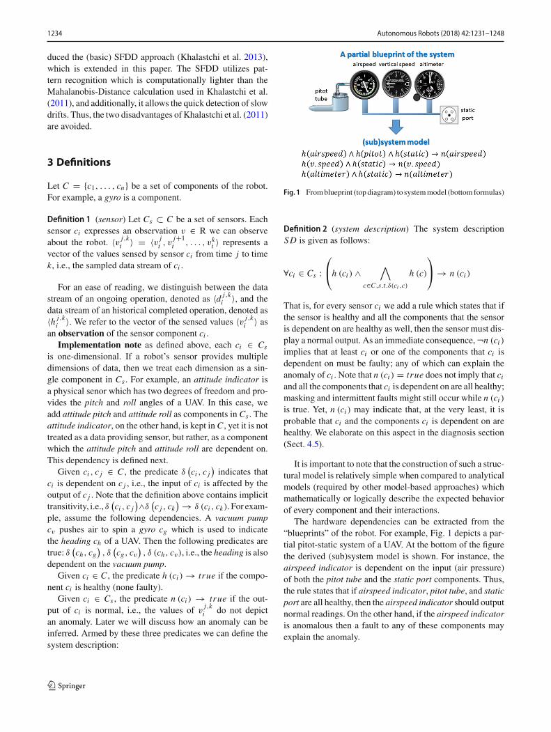
Fig. 1 Fromblueprint (top diagram) to systemmodel (bottom formulas)

Definition 2 (system description) The system descriptionSD is given as follows:

∀ci ∈ Cs :⎛

⎝h (ci ) ∧∧

c∈C,s.t .δ(ci ,c)

h (c)

⎞

⎠ → n (ci )

That is, for every sensor ci we add a rule which states that ifthe sensor is healthy and all the components that the sensoris dependent on are healthy as well, then the sensor must dis-play a normal output. As an immediate consequence,¬n (ci )

implies that at least ci or one of the components that ci isdependent on must be faulty; any of which can explain theanomaly of ci . Note that n (ci ) = true does not imply that ci

and all the components that ci is dependent on are all healthy;masking and intermittent faults might still occur while n (ci )

is true. Yet, n (ci ) may indicate that, at the very least, it isprobable that ci and the components ci is dependent on arehealthy. We elaborate on this aspect in the diagnosis section(Sect. 4.5).

It is important to note that the construction of such a struc-tural model is relatively simple when compared to analyticalmodels (required by other model-based approaches) whichmathematically or logically describe the expected behaviorof every component and their interactions.

The hardware dependencies can be extracted from the“blueprints” of the robot. For example, Fig. 1 depicts a par-tial pitot-static system of a UAV. At the bottom of the figurethe derived (sub)system model is shown. For instance, theairspeed indicator is dependent on the input (air pressure)of both the pitot tube and the static port components. Thus,the rule states that if airspeed indicator, pitot tube, and staticport are all healthy, then the airspeed indicator should outputnormal readings. On the other hand, if the airspeed indicatoris anomalous then a fault to any of these components mayexplain the anomaly.

123

Autonomous Robots (2018) 42:1231–1248 1235

A fundamental building block of the fault detection algo-rithms, proposed in the next section, is the ability to detectcorrelated sensors.

Definition 3 (correlated sensors) Given ci , c j ∈ CS , thepredicate σ

(ci , c j

) → true indicates that sensors ci andc j are correlated, that is, if their data streams are correlated.

The correlation function may vary. For instance, in ourimplementation we use the Pearson correlation calculation.The threshold above which the data streams are deemed ascorrelated may vary as well; in our experiments, for instance,we used 0.9. We address these issues in the description of theapproaches, and in the evaluation section.

A data stream may depict certain patterns, e.g., a “stuck”pattern where all the values in the data stream are the same.We define � as the set of patterns. In our implementations� = {stuck, dri f t}, i.e., patterns that might express faultsymptoms.

Definition 4 (pattern detection) Let the predicate

π(〈v j,k

i 〉, x)

→ true if the data stream 〈v j,ki 〉 is depicting

a pattern x ∈ �.

For instance, π(〈dt−m,t

i 〉, “stuck′′)is true if all the values

in the data stream of component ci in the last m time steps

are the same. π(〈dt−m,t

i 〉, “dri f t ′′)is true if, after a point in

time, the derivative of the values in the data stream appears toincrease (or decrease) towards a steeper angle. To make thecalculation simple and robust to noise in the data, we simplychecked if all the values are linearly arranged within a boundin an angle that is steeper than the one before (see Fig. 2).

Note that the patterns are domain specific and serve asinputs to the fault detection algorithm and are not the focusof this paper. Similarly, other patterns can be added, such as“abrupt change”, “drop to zero”, “static noise”, etc. if theymight express fault symptoms in other domains, e.g., (Nasa2009; Hashimoto et al. 2003; Sharma et al. 2010).

Fig. 2 An example of a “drift” detected. At time step 50 the valuesstated to drift w.r.t the values of time steps 1–49

Definition 5 (fault detection problem) Given a set of compo-nents C , an observation over Cs and the system description,the fault detection problem is to raise an alarm upon theoccurrence of a fault

4 The sensor-based fault detection anddiagnosis

In this sectionwe describe the SFDD and the extended SFDDapproaches. First, the fault detection process is discussed. Inparticular, we describe the SFDD, discuss its drawbacks andcontinue with the description of the extended SFDD faultdetection approach. Then, we describe the diagnosis process,which is the same for both approaches. Finally, we summa-rize by comparing the two approaches and hypothesizewhichshould be more accurate.

4.1 The basic SFDD approach

The SFDD (Khalastchi et al. 2013) is an online approach.The sensor readings are sampled at a fixed rate and stored ina ‘sliding window’. That is, for every time step t we storethe observation of the last m readings of every sensor—[〈dt−m,t

1 〉, . . . , 〈dt−m,tn 〉

]. Sensors may allow different sam-

pling rates. For sensors with a slower sampling rate theprevious value is repeated until a new value is sampled. Forsensors with a quicker sampling rate we simply neglect thedata in between the fixed samples. We advise to use the high-est sampling rate your robot can handle.

We assume that the robot starts with a non-faulty state,and a fault might occur after a given point in time. Thus, eachinstance of the sliding window (time step t) is divided into

twohalves.Thefirst half,[〈dt−m,t−m/2

1 〉, . . . , 〈dt−m,t−m/2n 〉

],

which ismade of older data samples, is assumed to contain no

faults. The second half[〈dt−m/2,t

1 〉, . . . , 〈dt−m/2,tn 〉

], which

is made of newer data samples, is checked for faults.The underlying assumption is that correlated sensors

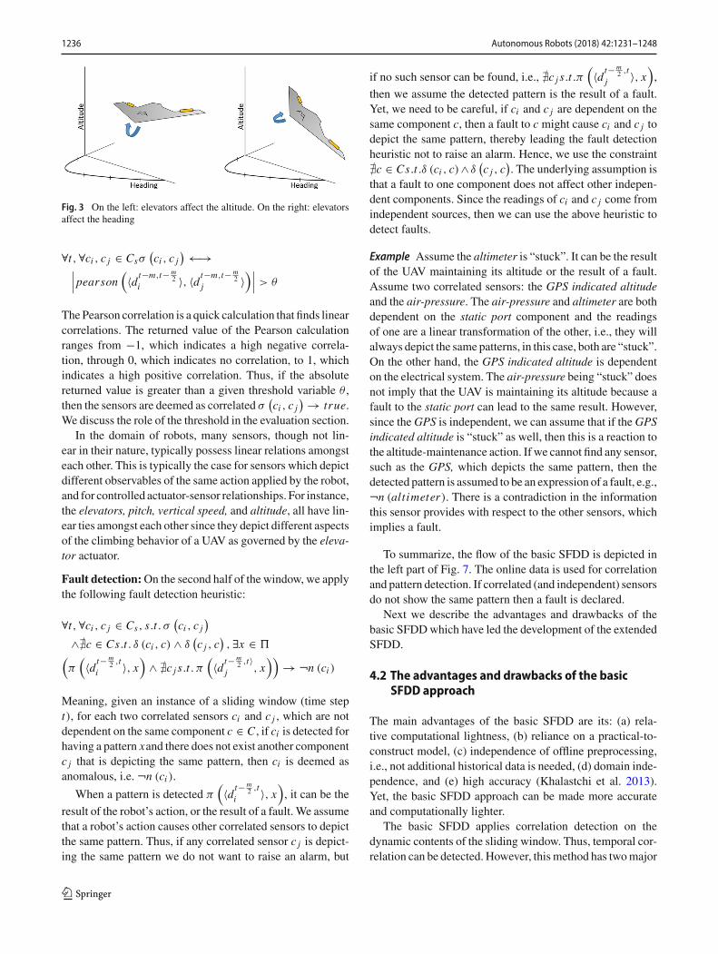
should stay correlated unless a fault has occurred or the robothas changed its behavior; the correlation between sensors isdynamic in nature. For instance, elevating the UAV typicallygains altitude, but if the UAV is rolled on its side then itwill accelerate its heading change rather than its altitude (seeFig. 3). In this behavior the heading rate of change, ratherthan the altitude climb, is correlated to the force applied onthe elevators.

Correlation detection Thus, on the first half of the windowwe check for correlations between each two sensors. Thatis, the correlation calculation is applied on dynamic content,and thus provides the information of dynamic correlations.To this end we used the Pearson correlation calculation.

123

1236 Autonomous Robots (2018) 42:1231–1248

Fig. 3 On the left: elevators affect the altitude. On the right: elevatorsaffect the heading

∀t,∀ci , c j ∈ Csσ(ci , c j

) ←→∣∣∣pearson

(〈dt−m,t− m

2i 〉, 〈dt−m,t− m

2j 〉

)∣∣∣ > θ

ThePearson correlation is a quick calculation that finds linearcorrelations. The returned value of the Pearson calculationranges from −1, which indicates a high negative correla-tion, through 0, which indicates no correlation, to 1, whichindicates a high positive correlation. Thus, if the absolutereturned value is greater than a given threshold variable θ ,then the sensors are deemed as correlated σ

(ci , c j

) → true.We discuss the role of the threshold in the evaluation section.

In the domain of robots, many sensors, though not lin-ear in their nature, typically possess linear relations amongsteach other. This is typically the case for sensors which depictdifferent observables of the same action applied by the robot,and for controlled actuator-sensor relationships. For instance,the elevators, pitch, vertical speed, and altitude, all have lin-ear ties amongst each other since they depict different aspectsof the climbing behavior of a UAV as governed by the eleva-tor actuator.

Fault detection:On the second half of the window, we applythe following fault detection heuristic:

∀t,∀ci , c j ∈ Cs, s.t . σ(ci , c j

)

∧�c ∈ Cs.t . δ (ci , c) ∧ δ(c j , c

), ∃x ∈ �

(π

(〈dt− m

2 ,ti 〉, x

)∧ �c j s.t . π

(〈dt− m

2 ,t〉j , x

))→ ¬n (ci )

Meaning, given an instance of a sliding window (time stept), for each two correlated sensors ci and c j , which are notdependent on the same component c ∈ C , if ci is detected forhaving a pattern xand there does not exist another componentc j that is depicting the same pattern, then ci is deemed asanomalous, i.e. ¬n (ci ).

When a pattern is detected π(〈dt− m

2 ,ti 〉, x

), it can be the

result of the robot’s action, or the result of a fault. We assumethat a robot’s action causes other correlated sensors to depictthe same pattern. Thus, if any correlated sensor c j is depict-ing the same pattern we do not want to raise an alarm, but

if no such sensor can be found, i.e., �c j s.t .π(〈dt− m

2 ,tj 〉, x

),

then we assume the detected pattern is the result of a fault.Yet, we need to be careful, if ci and c j are dependent on thesame component c, then a fault to c might cause ci and c j todepict the same pattern, thereby leading the fault detectionheuristic not to raise an alarm. Hence, we use the constraint�c ∈ Cs.t .δ (ci , c)∧ δ

(c j , c

). The underlying assumption is

that a fault to one component does not affect other indepen-dent components. Since the readings of ci and c j come fromindependent sources, then we can use the above heuristic todetect faults.

Example Assume the altimeter is “stuck”. It can be the resultof the UAV maintaining its altitude or the result of a fault.Assume two correlated sensors: the GPS indicated altitudeand the air-pressure. The air-pressure and altimeter are bothdependent on the static port component and the readingsof one are a linear transformation of the other, i.e., they willalways depict the same patterns, in this case, both are “stuck”.On the other hand, the GPS indicated altitude is dependenton the electrical system. The air-pressure being “stuck” doesnot imply that the UAV is maintaining its altitude because afault to the static port can lead to the same result. However,since the GPS is independent, we can assume that if the GPSindicated altitude is “stuck” as well, then this is a reaction tothe altitude-maintenance action. If we cannot find any sensor,such as the GPS, which depicts the same pattern, then thedetected pattern is assumed to be an expression of a fault, e.g.,¬n (altimeter). There is a contradiction in the informationthis sensor provides with respect to the other sensors, whichimplies a fault.

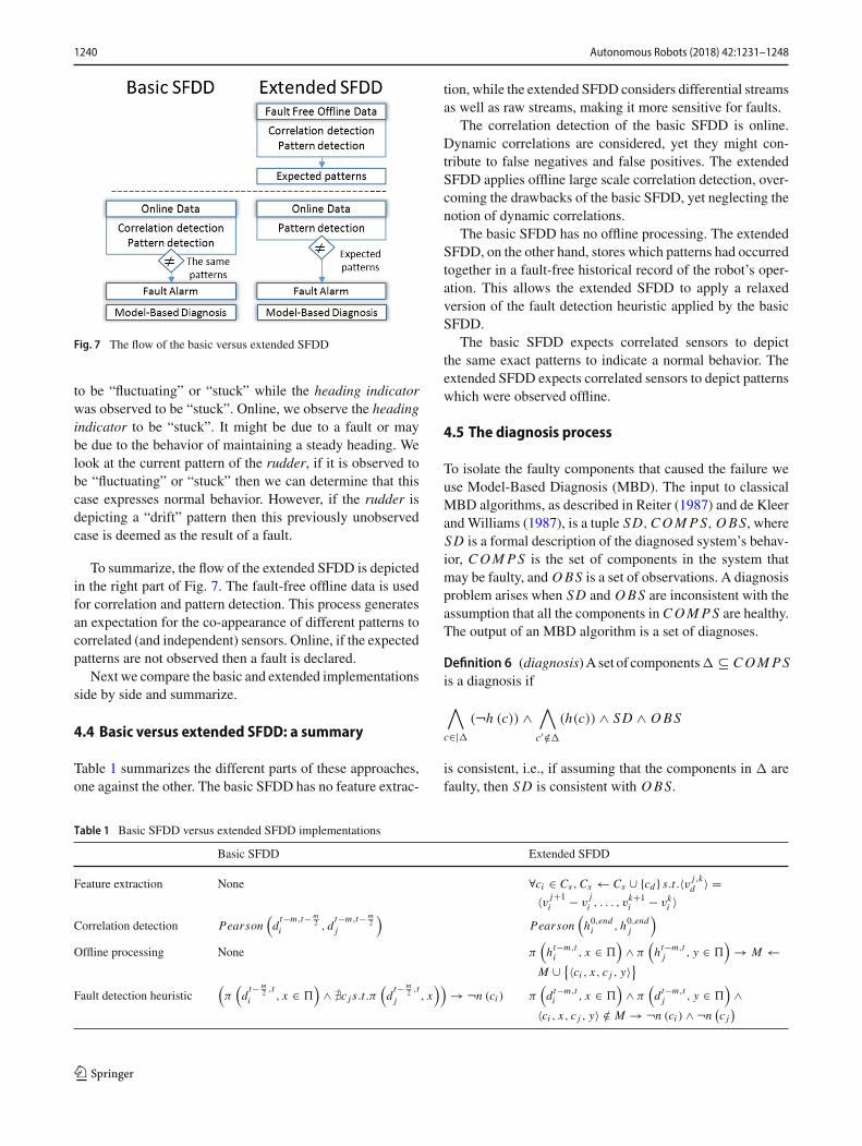
To summarize, the flow of the basic SFDD is depicted inthe left part of Fig. 7. The online data is used for correlationand pattern detection. If correlated (and independent) sensorsdo not show the same pattern then a fault is declared.

Next we describe the advantages and drawbacks of thebasic SFDDwhich have led the development of the extendedSFDD.

4.2 The advantages and drawbacks of the basicSFDD approach

The main advantages of the basic SFDD are its: (a) rela-tive computational lightness, (b) reliance on a practical-to-construct model, (c) independence of offline preprocessing,i.e., not additional historical data is needed, (d) domain inde-pendence, and (e) high accuracy (Khalastchi et al. 2013).Yet, the basic SFDD approach can be made more accurateand computationally lighter.

The basic SFDD applies correlation detection on thedynamic contents of the sliding window. Thus, temporal cor-relation can be detected. However, thismethod has twomajor

123

Autonomous Robots (2018) 42:1231–1248 1237

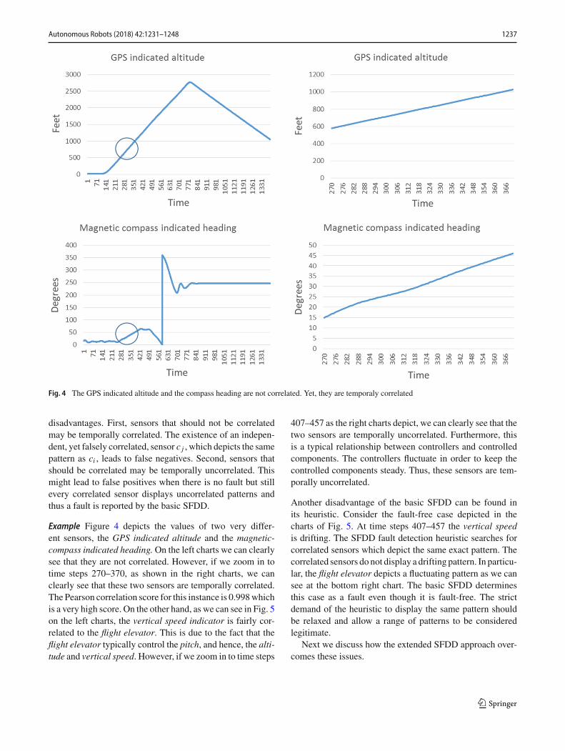
Fig. 4 The GPS indicated altitude and the compass heading are not correlated. Yet, they are temporaly correlated

disadvantages. First, sensors that should not be correlatedmay be temporally correlated. The existence of an indepen-dent, yet falsely correlated, sensor c j , which depicts the samepattern as ci , leads to false negatives. Second, sensors thatshould be correlated may be temporally uncorrelated. Thismight lead to false positives when there is no fault but stillevery correlated sensor displays uncorrelated patterns andthus a fault is reported by the basic SFDD.

Example Figure 4 depicts the values of two very differ-ent sensors, the GPS indicated altitude and the magnetic-compass indicated heading. On the left charts we can clearlysee that they are not correlated. However, if we zoom in totime steps 270–370, as shown in the right charts, we canclearly see that these two sensors are temporally correlated.The Pearson correlation score for this instance is 0.998whichis a very high score. On the other hand, as we can see in Fig. 5on the left charts, the vertical speed indicator is fairly cor-related to the flight elevator. This is due to the fact that theflight elevator typically control the pitch, and hence, the alti-tude and vertical speed. However, if we zoom in to time steps

407–457 as the right charts depict, we can clearly see that thetwo sensors are temporally uncorrelated. Furthermore, thisis a typical relationship between controllers and controlledcomponents. The controllers fluctuate in order to keep thecontrolled components steady. Thus, these sensors are tem-porally uncorrelated.

Another disadvantage of the basic SFDD can be found inits heuristic. Consider the fault-free case depicted in thecharts of Fig. 5. At time steps 407–457 the vertical speedis drifting. The SFDD fault detection heuristic searches forcorrelated sensors which depict the same exact pattern. Thecorrelated sensors do not display a drifting pattern. In particu-lar, the flight elevator depicts a fluctuating pattern as we cansee at the bottom right chart. The basic SFDD determinesthis case as a fault even though it is fault-free. The strictdemand of the heuristic to display the same pattern shouldbe relaxed and allow a range of patterns to be consideredlegitimate.

Next we discuss how the extended SFDD approach over-comes these issues.

123

1238 Autonomous Robots (2018) 42:1231–1248

Fig. 5 The vertical speed indicator and the fligjt elevator ar correlated. Yet, they are temporaly not correlated

4.3 The extended SFDD approach

Understanding the drawbacks of the basic SFDD has pavedtheway for the addition of extended features that improve thebasic SFDD.Wedenote this implementation as the “extendedSFDD”. The following features make the extended SFDDmore accurate and computationally lighter than the basicSFDD.

Feature extraction The extended SFDD applies a simpleprocess of differential feature extractionwhich allows greatersensitivity for the occurrence of faults.

∀ci ∈ Cs, Cs ← Cs ∪ {cd} s.t .〈v j,kd 〉

= 〈v j+1i − v

ji , v

j+2i − v

j+1i , . . . , vk+1

i − vki 〉

For each sensor ci we add to the set of sensors Cs a virtualsensor cd which is comprised from the differentials of theraw readings of ci .

The SFDD approach is only sensitive to sensors that arecorrelated to other sensors. The use of both raw and differ-ential streams allow the discovery of additional correlations,

specifically actuator-sensor relationships, thereby increasingthe extended SFDD’s sensitivity for faults.

The sensors of a robot continuously sense the state of therobot and its environment—before and after an actuator isapplied. Thus, the differential readings of a sensor may becorrelated to the raw readings of an actuator, indicating theactuator’s effect. Figure 6 depicts an example. The flight ele-vator (top left chart) is not correlated to any other sensor, andin particular, thealtimeter (right chart).Yet, theflight elevatoris one of the most significant actuators that governs the alti-tude. Thankfully, the differential data stream of the altimeter(bottom chart) is correlated to the flight elevator, exposingthe relationship between the two. Now, the extended SFDDis sensitive to faults that might occur to the flight elevator.

Correlation detection The correlation detection process isperformed offline, on a fault-free complete historical record,i.e.

σ(ci , c j

) ←→∣∣∣pearson

(〈h0,end

i 〉, 〈h0,endj 〉

)∣∣∣ > θ

This solves the problems of unwanted temporal correlationsbetween uncorrelated sensors, and unwanted temporal mis-

123

Autonomous Robots (2018) 42:1231–1248 1239

Fig. 6 The Flight elevator actuator is uncorrelated to the altimeter, but is correlated to the altimeter’s differential data

correlations between correlated sensors. Sensors are deemedas correlated only if they are correlated in the large scaleof an entire operation; small scale temporal correlations ormiscorrelations become insignificant in the large scale.

In addition, since the correlationdetection is anofflinepro-cess, the online computational load is decreased. However,the extended SFDD neglects the notion of dynamic correla-tions, and thus which approach is more accurate becomes aninteresting question, which we address this paper.

Fault detection The fault detection heuristic is relaxed, andallows the co-appearance of different patterns to indicate anormal behavior.

We define M to be a set of observations where each obser-vation is a tuple of the form 〈ci , x, c j , y〉 where ci , c j ∈ Cs

and x, y ∈ �.The denotation of the tuple is that the occurrence of pat-

tern x to component ci and pattern yto component c j wereobserved at the same time. For instance, ci is the altime-ter sensor, c j is the GPS indicated altitude, x and y are the“stuck” pattern. Both sensors were observed to be stuck atthe same time.

Offline, we process the fault-free historical record in asliding window fashion (sized m), and for each instance ofthe window (time step t)we examine correlated sensor com-ponents. For each two correlated sensors ci and c j , whichare not dependent on the same component c, if patterns

x, y are detected for ci , c j respectively, then the observation〈ci , x, c j , y〉 is added to M .

Formally:

∀t,∀ci , c j ∈ Cs , s.t . σ(ci , c j

) ∧ �c ∈ C s.t . δ (ci , c) ∧ δ(c j , c

),

π(〈ht−m,t

i 〉, x ∈ �)

∧ π(〈ht−m,t

j 〉, y ∈ �)

→M ← M ∪ {〈ci , x, c j , y〉}

We treat M as a set of legitimate observations. Online, weapply a similar process, yet if the detected observation doesnot exist in M then we raise a fault alarm.

Formally:

∀t,∀ci , c j ∈ Cs , s.t . σ(ci , c j

) ∧ �c ∈ Cs.t .δ (ci , c) ∧ δ(c j , c

),

(π

(〈dt−m,t

i 〉, x ∈ �)

∧ π(〈dt−m,t

j 〉, y ∈ �)

∧ 〈ci , x, c j , y〉 /∈ M)

→ ¬n (ci ) ∧ ¬n(c j

)

In other words, if a combination of patterns appears onlineto correlated and independent sensors ci , c j , then if it wasobserved in the fault-free record then this case is deemed asnormal, otherwise, both sensors are deemed as anomalous,i.e., ¬n (ci ) ∧ ¬n

(c j

).

Example The rudder controls the yaw axis of the UAV andthus its heading. Offline, we observed a behavior ofmaintain-ing a steady heading. The state of the rudder was observed

123

1240 Autonomous Robots (2018) 42:1231–1248

Fig. 7 The flow of the basic versus extended SFDD

to be “fluctuating” or “stuck” while the heading indicatorwas observed to be “stuck”. Online, we observe the headingindicator to be “stuck”. It might be due to a fault or maybe due to the behavior of maintaining a steady heading. Welook at the current pattern of the rudder, if it is observed tobe “fluctuating” or “stuck” then we can determine that thiscase expresses normal behavior. However, if the rudder isdepicting a “drift” pattern then this previously unobservedcase is deemed as the result of a fault.

To summarize, the flow of the extended SFDD is depictedin the right part of Fig. 7. The fault-free offline data is usedfor correlation and pattern detection. This process generatesan expectation for the co-appearance of different patterns tocorrelated (and independent) sensors. Online, if the expectedpatterns are not observed then a fault is declared.

Next we compare the basic and extended implementationsside by side and summarize.

4.4 Basic versus extended SFDD: a summary

Table 1 summarizes the different parts of these approaches,one against the other. The basic SFDD has no feature extrac-

tion, while the extended SFDD considers differential streamsas well as raw streams, making it more sensitive for faults.

The correlation detection of the basic SFDD is online.Dynamic correlations are considered, yet they might con-tribute to false negatives and false positives. The extendedSFDD applies offline large scale correlation detection, over-coming the drawbacks of the basic SFDD, yet neglecting thenotion of dynamic correlations.

The basic SFDD has no offline processing. The extendedSFDD, on the other hand, stores which patterns had occurredtogether in a fault-free historical record of the robot’s oper-ation. This allows the extended SFDD to apply a relaxedversion of the fault detection heuristic applied by the basicSFDD.

The basic SFDD expects correlated sensors to depictthe same exact patterns to indicate a normal behavior. Theextended SFDD expects correlated sensors to depict patternswhich were observed offline.

4.5 The diagnosis process

To isolate the faulty components that caused the failure weuse Model-Based Diagnosis (MBD). The input to classicalMBD algorithms, as described in Reiter (1987) and de Kleerand Williams (1987), is a tuple SD, C O M P S, O BS, whereSD is a formal description of the diagnosed system’s behav-ior, C O M P S is the set of components in the system thatmay be faulty, and O BS is a set of observations. A diagnosisproblem arises when SD and O BS are inconsistent with theassumption that all the components in C O M P S are healthy.The output of an MBD algorithm is a set of diagnoses.

Definition 6 (diagnosis)A set of components� ⊆ C O M P Sis a diagnosis if

∧

c∈|�(¬h (c)) ∧

∧

c′ /∈�

(h(c)) ∧ SD ∧ O BS

is consistent, i.e., if assuming that the components in � arefaulty, then SD is consistent with O BS.

Table 1 Basic SFDD versus extended SFDD implementations

Basic SFDD Extended SFDD

Feature extraction None ∀ci ∈ Cs , Cs ← Cs ∪ {cd } s.t .〈v j,kd 〉 =

〈v j+1i − v

ji , . . . , vk+1

i − vki 〉

Correlation detection Pearson(

dt−m,t− m

2i , d

t−m,t− m2

j

)Pearson

(h0,end

i , h0,endj

)

Offline processing None π(

ht−m,ti , x ∈ �

)∧ π

(ht−m,t

j , y ∈ �)

→ M ←M ∪ {〈ci , x, c j , y〉}

Fault detection heuristic(π

(d

t− m2 ,t

i , x ∈ �)

∧ �c j s.t .π(

dt− m

2 ,tj , x

))→ ¬n (ci ) π

(dt−m,t

i , x ∈ �)

∧ π(

dt−m,tj , y ∈ �

)∧

〈ci , x, c j , y〉 /∈ M → ¬n (ci ) ∧ ¬n(c j

)

123

Autonomous Robots (2018) 42:1231–1248 1241

The set of components (C O M P S) in our domain is C .The system description (SD) has been formally defined inDefinition 2. The observation is the data stream of the sensorcomponents (Definition 1). However, to useMBDalgorithmswe should express the observation as Boolean variables. Infact, we have defined the predicate n (c) which returns trueif the output of component c is normal. Thus, we can defineOBSwith this predicate on the output of the sensors: O BS =∧

c∈CSn (c). The values of n (c) for the sensor components

will be computed before the diagnosis process by the faultdetection process described in the previous section.

A known approach to compute diagnoses is conflictdirected. A conflict directed approach identifies first con-flict sets, each of which includes at least one fault. Then, itapplies a hitting set algorithm to compute sets of multiplefaults that explain the observation (de Kleer and Williams1987; Williams and Ragno 2007; Stern et al. 2012). Intu-itively, since at least one component in every conflict is faulty,only a hitting set of all conflicts can explain the unexpectedobservation. Note that inferring conflicts in our model isstraightforward: for each observation that returns f alse, aconflict includes all the components that their output influ-ence that observation. Obviously, it is logically inferred fromthe model.

Barinel is a recently proposed MBD algorithm (Abreuet al. 2009, 2011) based on exactly this concept. The maindrawback of using Barinel is that it often outputs a large setof diagnoses, thus providing weaker guidance to the operatorthat is assigned to solve the observed fault.

To address this problem, Barinel computes a score forevery diagnosis it returns, estimating the likelihood that itis true. This serves as a way to prioritize the large set ofdiagnoses returned by Barinel. The exact details of how thisscore is computed is given by Abreu et al. For the purpose ofthis paper, it is important to note that the score computationused byBarinel is Bayesian: it computes for a given diagnosisthe posterior probability that it is correct given the n and ¬nobservations. In this work we also consider the results of theobservations to rank the diagnoses.

For example, consider the subsystem depicted in Fig. 1,and that the airspeed indicator readings are stuck. Accord-ing to the model ¬n (altimeter) → ¬h (altimeter) ∨¬h (pitot) ∨ ¬h (static). Thus, the conflict is {altimeter ,

pitot, static}. However, since the readings of the verti-cal speed and altimeter are normal, the probability thatthe static port is faulty is decreased, thereby returning� ={{airspeed}, {pitot}}.

5 Evaluation

In this section we provide our evaluation: the experimentalsetup, competing approaches, evaluation measurements andthe results.

5.1 Experimental setup

We created a new data set which we contribute as a pub-lic benchmark for general fault detection and diagnosisapproaches as well as approaches designed more specifi-cally for the domain of robots. We utilized the FlightGear(Perry 2004) flight simulator. FlightGear is an open sourcehigh fidelity flight simulator designed for research purposeand is used for a variety of research topics. FlightGear isa great domain for robotic FDD research, particularly forUAVs, and yet it is not used enough for this topic of research.We thoroughly introduce this domain, and use it as our maintestbed. In addition to this simulated domain, we experimentwith two real-world domains as well: a commercial UAVand a laboratory robot. These domains are not as intricateas the FlightGear domain, but they do provide the differentaspects of real-world data, and thus, appliance of the FDDapproaches to the real-world domains.

5.1.1 The FlightGear benchmark domain

The most important aspect of FlightGear as a domain forFDD is the fact that FlightGear has built-in realistically sim-ulated sensors, internal components, engine, and actuatorsfaults. For example, if the vacuum fails, the HSI (Hori-zontal Situation Indicator) gyros spin down slowly with acorresponding degradation in response as well as a slowlyincreasing bias/error (drift) (Perry 2004), and in turn, if notdetected, lead the aircraft miles away from its desired posi-tion. Thus, the first advantage is that FDD approaches maysolve a real-world problem.More importantly, while in otherdomains faults’ expressions are injected into the recordeddata after the flight is done, in FlightGear the simulated faultsare built-in and can be injected during the flight. First, thereis no bias; the faults were not modeled by the scientist whocreated and tested the FDD approach. Second, built-in faultswhich are injected during the flight propagate and affect thewhole simulation. Hence, fault expressions are more realis-tic.

We created a control software to fly a Cessna 172p air-craft as an autonomous UAV. The flight instruments are usedas sensors which sense the aircraft state with respect to itsenvironment. These sensor readings are fed into a decisionmaking mechanism which issues instructions to the flightcontrols (actuators) such that goals are achieved. As the UAVoperates, its state is changed and again being sensed by itssensors. The desired flight pattern consists of seven steps: atakeoff, 30 s of a strait flight, a right turn of 45◦, 15 s of astrait flight, a left turn of 180◦, 15 s of a strait flight, and adecent to one kilofeet. In total, the flight pattern duration is6min of fight.

During a flight, 23 sensors are sampled in a frequency of4Hz. These sensors present 5 flight controls feedback (actua-

123

1242 Autonomous Robots (2018) 42:1231–1248

Table 2 Summary of injectedfaults

Fault to Type Effect

1 Airspeed indicator Sensor Stuck

2 Altimeter

3 Compass

4 Turn indicator Quick drift to minimumvalue

5 Heading indicator Stuck

6 Vertical speed indicator

7 Slip skid ball

8 Pitot tube Internal component Airspeed drifts up

9 Static port Airspeed drifts Altimeterand Encoder are stuck

10 Electrical Turn indicator slowly driftsdown

11 Vacuum Attitude and headingindicators slowly drift

12 Elevator Actuator Stuck

tors), and 18 flight instruments (sensors). The sampled flightcontrols are the ailerons, elevators, rudder, flaps, and enginethrottle. The flight instruments are the airspeed indicator,altimeter, horizontal situation indicator, encoder, GPS, mag-netic compass, slip skid ball, turn indicator, vertical speedindicator, and engine’s RPM. Each instrument yields 1 to 4streams of data which together add up to 18 sensors. Notethat we did not sample sensors that would have made thefault detection easy. For instance, sampling the current andvoltage of the aircraft would have made the detection of anelectrical system failure unchallenging.

The data set contains one flight which is free of faults, 5subsets that each contains 12 recorded flights in which dif-ferent faults were injected, and one special “stunt flight”. Intotal, the data set contains 62 recorded flights with almost90,000 data instances. We injected faults to 7 different sen-sors, 4 different internal components, and an actuator. Table 2depicts the different faults and their effect. For instance, afault injection of type 9 fails the static port which, in turn,leads the airspeed indicator to drift upwards or downwards,and the altimeter and encoder to be stuck.

Four subsets represent a single fault scenario. Each ofthe 12 flights in a subset corresponds to an injected fault inTable 2, i.e., flight 1 was injected with an airspeed indicatorfailure, flight 2 was injected with an altimeter failure, etc.Flights 1–9 were injected 6 times with faults. Each injectionoccurred at a random time of the flight, and for a randomduration of 5–30s. Flights 10, 11 were injected once, at arandom time of the flight, with a duration of 180s. Theseflights depict a slow and shallow drift which develops overtime. The twelfth flight was injected three times with a faultto the flight elevator actuator, where each fault occurs at arandom time and has a duration of 30s.

The fifth subset represents a double-fault scenario. In eachof the 12 flights we injected 3 times double faults. Each timea fault was injected to two different components at the sametime. The double injection occurred at a random time of theflight, and for a random duration of 10–30s. In total, the dataset contains 72 injected faults.

In addition to these five subsets of flights we recorded aspecial “stunt flight” which has a significantly different flightpattern than the other flights in the benchmark. The stuntflight includes high-G maneuvers, i.e., sharp turns, climbs,dives, and loops where axis change is highly frequent. Whilethe aircraft is rolled to its side, turning sharply, a fault wasinjected to the altimeter which causes the indicated altitudeto be stuck. The quick transitions between states make thisflight very challenging for FDD approaches, especially forapproaches which are depended on offline learning, like theextended SFDD, where state transitions were mild.

5.1.2 Real-world domains

In addition to the FlightGear simulated domain, we exper-iment with two physical robots: a commercial UAV and alaboratory robot. These domains are not as complex as thesimulated domain, but they serve to show the domain inde-pendence of the SFDD and its ability to handle real-worlddata.

CommercialUAVdomainThe realUAVdomain consistsof 6 recorded real flights of a commercial UAV. 53 sensorswere sampled in 10Hz. The sensors consists of telemetry,inertial, engine and servos data. Flights duration varies from37 to 71min. The UAVmanufacture injected a synthetic faultto two of the flights. The first scenario is a value that driftsdown to zero. The second scenario is a value that remains

123

Autonomous Robots (2018) 42:1231–1248 1243

frozen (stuck). The detection of these two faults were chal-lenging for themanufacture since in both scenarios the valuesare in normal range. These two flights were used to test theFDD approaches. In total, the test flights contain 65,741 datainstances out of which 1,593 are expression of faults.

Laboratory robot domain Robotican is a laboratoryrobot that has 2 wheels, 3 sonar range detectors in the front,and 3 infrared range detectors which are located right abovethe sonars, making the sonars and infrareds redundant sys-tems to one another. This redundancy reflects real worlddomains such as unmanned vehicles. In addition, Roboti-can1 has 5 degrees of freedom arm. Each joint is held by twoelectrical motors. These motors provide a feedback valuedepicting the voltage that was actually applied.

The following scenario was repeated 10 times: the robotslows its movement as it approaches a cup. Concurrently, therobot’s arm is adjusted to grasp the cup. In 9 out of the 10times faults were injected. Faults of type stuck or drift wereinjected to different type of sensors (motor voltage, infraredand sonar). We sampled 15 sensors in 8Hz. Scenarios dura-tion lasted only 10s where 1.25 s expressed a fault. In total,the test set contains 800 instances out of which 90 are expres-sion of faults.

5.1.3 Competing fault detection approaches

We carefully chose three competing approaches, where eachapproach is similar to the SFDD in some aspect, but empha-sizes the difference of other aspects. Table 3 depicts thecompeting approaches, their similarities anddifferences formthe SFDD, and the hypothesis for their ability to detect faultsaccurately.

The extended SFDD uses an offline fault-free data set to“learn” which patterns may co-appear. Classification algo-rithms can utilize such information as well. The SVM is awell-knownand typically successful classification algorithm.In addition, we provide the SVM based approach with bothfaulty and normal examples. Yet, we expect the SVM to fail,i.e., to report every fault as normal. Our experiment containsinjected faults of contextual nature, and thus, domain knowl-edgemaybe needed. TheSVMis domain-independent,whilethe SFDD’s fault detection heuristic utilizes domain knowl-edge (component dependencies). In addition, the context isimplicitly provided to the SFDD in the form of the sliding

window and correlated sensors. The SVM approach does notcluster correlated sensors together. In turn, uncorrelated datainstances form a scattered distribution that require large mar-gins from the support vectors. These large margins reducethe fault detection sensitivity to the point where almost everydata instance would be considered as normal.

Another aspect of the SFDD is the dependency on lin-ear correlations. If two sensors depict a linear correlationthen the readings of one sensor can be used to predict thereadings of the other. To this end, linear regression can beused offline to learn these linear ties from a fault-free record.However, online, the observed values are distributed aroundthe model’s predicted values. A threshold needs to be setsuch that all normal data instances fall within this thresh-old. Since the readings of one sensor are actually affectedby several others, then large deviations from the predictedvalue are expected. For instance, the vertical speed cannot beaccurately predicted by the readings of the pitch angle sincethe vertical speed is affected by the current altitude and air-speed as well. As a result, higher thresholds are set, leadingto undetected faults. On the other hand, the SFDD avoids thisproblem since it concerns patterns and not expected values.

Our previous approach (Khalastchi et al. 2011), OnlineData Driven Anomaly Detection (ODDAD), is very simi-lar to the SFDD. The online data is processed via a slidingwindow and sensors are grouped together according to theirlinear correlations. Yet, the fault detection heuristic is dif-ferent. ODDAD uses the model-free Mahalanobis-Distancecalculation (Mahalanobis 1936) to indicate anomalies. TheSFDD applies a fault detection heuristic that utilizes domain-knowledge (component dependencies). Thus, we expect theSFDD approaches to be more accurate than ODDAD.

5.1.4 Evaluation measurements

The main measurement we are interested in is how accuratean FDD approach is. For that, we define the following com-mon parameters about a fault report, which Table 4 depicts.

Every detected fault counts as one true positive. Everyfalse alarm counts as one false positive. Every undetectedfault counts as a false negative, and the rest counts as truenegatives, i.e., no faults and no alarm. The fault detectionrate (a.k.a. recall, true positive rate, sensitivity) is defined as= T P

T P+F N whereTP is the amount of true positives, andFN is

Table 3 The competingapproaches, theirs similarities,differences and hypothesiscompared to the SFDD

SVM Linear Regression ODDAD

Similarity Offline learning Linear relations Correlation based

Difference Classification versus faultdetection heuristic

Value prediction versuspattern prediction

Model free versusmodel based

Hypothesis Undetected contextualfaults

Threshold settingproblem

Lower fault detectionrate

123

1244 Autonomous Robots (2018) 42:1231–1248

Table 4 Evaluation measures

Evaluation measure Description

Fault detection rate The rate of faults detected out ofall injected faults

False alarm rate The rate of incorrect fault reportsout of all none-faults

F Ptime The average duration of incorrectfault reports

Detection time lag The time it takes an FDD approachto detect a fault

Diagnosis Precision and true positive rate

the amount of false negatives. The false alarm rate (a.k.a. falsepositive rate, 1—specificity) is defined as = F P

T N+F P whereFP is the amount of false positives and TN is the amount oftrue negatives. A perfect FDD approach has a detection rateof 1 (all faults are detected) and a false alarm rate of 0 (nofalse alarms).

Knowing the false alarm rate of an approach is not enough.An approachmight theoretically have only one incorrect faultreport, but this report has a duration of the entire operation.Hence, we measure the average duration of incorrect faultreports denoted as F Ptime. An FDD approach with a lowerscore is better.

As we have mentioned in the introduction, an FDDapproach can benefit from being quick, i.e., detect the faultas quickly as possible as it occurs. Thus, another importantanalysis is the (average) time lag between the occurrence of afault and its detection by an FDD approach. In particular, thisis interesting for theflights 10 and11 in theFlightGear bench-mark, where the expression of the fault progresses slowly.

For the evaluation of the diagnosis we first need to definewhich diagnosis is returned. Since the diagnoses are rankedaccording to their probabilities, we simply choose the firstdiagnosis that is ranked first. The selected diagnosis is a setof components which supposed to be faulty. For each faultycomponent that is not included in this set we count one falsenegative (FN). For each faulty component that is included inthe set we count one true positive (TP). For each componentincluded in the set, which is not faulty we count one falsepositive (FP). Hence, we are interested in twomeasurements:The diagnosis precision defined as T P

T P+F P , and the diagnosis

true positive rate defined as T PT P+F N .

For example, assume that the diagnosis for injected faultsto the vertical speed indicator and the static port is {staticport}. Thus, TP=1, FN=1. In a case that the diagnosis for apitot tube failure is {airspeed indicator}, TP=0, FP=1.

5.2 Results and analysis

In this section we provide our analysis and results. We startwith the comparison of the competing approaches. We con-

tinue with an analysis of the contribution of each feature ofthe SFDD.We concludewith a summary of conclusions fromthe results.

5.2.1 The results of the competing approaches

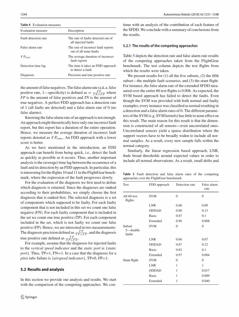
Table 5 depicts the detection rate and false alarm rate resultsof the competing approaches taken from the FlightGearbenchmark. The test column depicts the test flights fromwhich the results were taken.

We present results for (1) all the five subsets, (2) the fifthsubset—the multiple fault scenarios, and (3) the stunt flight.For instance, the false alarm rate of the extended SFDDmea-sured over the entire 60 test flights is 0.008. As expected, theSVM based approach has failed to detect the faults. Eventhough the SVM was provided with both normal and faultyexamples, every instancewas classified as normal resulting ina detection and a false alarm rates of 0. The different parame-ters of the SVM(e.g. SVMkernels) has little to none effect onthis result. The main reason for this result is that the dimen-sion is constructed of all sensors—even uncorrelated ones.Uncorrelated sensors yield a sparse distribution where thesupport vectors have to be broadly widen to include all nor-mal samples. As a result, every new sample falls within thenormal category.

Similarly, the linear regression based approach, LNR,finds broad thresholds around expected values in order toinclude all normal observations. As a result, small drifts and

Table 5 Fault detection and false alarm rates of the competingapproaches over the FlightGear benchmark

Test FDD approach Detection rate False alarmrate

All 60 testflights

SVM 0 0

LNR 0.68 0.09

ODDAD 0.88 0.13

Basic 0.87 0.1

Extended 0.96 0.008

Subset5—doublefaults

SVM 0 0

LNR 0.68 0.07

ODDAD 0.87 0.12

Basic 0.82 0.1

Extended 0.97 0.004

Stunt flight SVM 0 0

LNR 1 1

ODDAD 1 0.017

Basic 1 0.009

Extended 1 0.040

123

Autonomous Robots (2018) 42:1231–1248 1245

Table 6 Results on the real-world domains

Domain Approach Detection rate False alarm rate

Commercial UAV SVM 0 0

LNR 0 0.040

ODDAD 1 0.037

Basic 1 0.032

Extended 1 0.002

Robotican1 SVM 0 0

LNR 0.44 0.0035

ODDAD 1 0.017

Basic 0.56 0

Extended 1 0.012

stuck patterns fall within these thresholds and faults are leftundetected. In turn, the detection rate decreases. The falsealarm rate is quite high as well. Non-fault samples can stillbe outside of the calculated thresholds, as we cannot expectto observe every possible data instance in fault-free record.

For all test flights, the ODDAD approach and the basicSFDD have very similar scores, where the false alarm rateof the basic SFDD is a bit better. Compared to the SVM andLNR these scores are significantly better. The main reason isthat theODDADandbasic SFDDapproaches do group corre-lated sensors together, and each avoids the threshold-settingproblem of the SVM and LNR in a different way. ODDADcalculates for each group of correlated sensors a thresholdbased on the furthest Mahalanobis distance observed in thecurrent instance of the sliding window. The basic SFDDapplies pattern detection and thus it does not need to seta threshold above which a fault is detected. The reason thebasic SFDD has a bit lower (better) false alarm rate is due toits use of the structural model in the fault detection heuristic,which only considers independent correlated sensors.

The extended SFDD is significantly better than the com-peting approaches in all test flights except the stunt flight; theODDAD and basic SFDD show a lower false alarm rate. Thestunt flight significantly differs from fault-free flight, whichis quite leveled. The ODDAD and basic SFDD, which do notprocess anofflineoperation, have anatural advantageover theextended SFDD when the online operation significantly dif-fers from the offline operation. It can be interesting to devisea way to automatically decide online which implementationto use. We leave that to future work.

Similar resultswere obtained from the real-world domainsas Table 6 depicts. Once again the extended SFDD is sig-nificantly more accurate than the other approaches. Thedetection rate of the basic SFDD is surprisingly low for theRobotican1 domain—0.56. Since each operation lasted onlya few seconds, the size of the sliding window is kept small.Recall that the basic SFDD divides the sliding window into

Table 7 Contributions of different features of the SFDD (TPR,FPR)

Online Offline

Raw 0.87, 0.1 0.87, 0.005

Raw+Diff 0.89, 0.15 0.96, 0.008

two halves, providing even less data to work with. This mayexplain the low result.

The F Ptime measure for the FlightGear benchmark ofLNR, ODDAD, basic SFDD, and extended SFDD is 31, 20,8.9, and 6.5 s respectively. The extendedSFDDhas the lowest(best) score. These results show that both SFDD implemen-tations have small durations of incorrect fault reports as wellas having low false alarm rates.

5.2.2 The contribution of the SFDD features

We wish to show the contribution of each feature of theextended SFDD approach presented here. Table 7 depictsthe contribution of the following features. “Online” refers toonline (temporal) correlation detection and the basic SFDD’sfault detection heuristic. “Offline” refers to offline (largescale) correlation detection and the extended SFDD’s relaxedfault detection heuristic, which relies on offline observations.“Raw” refers to the raw sensor readings, “Raw+Diff” refersto the addition of differential data streams as extracted fea-tures. Each cell represents a fault detection rate and a falsealarm rate the approach scored. For example, the basic SFDDis represented by the cell for {Online, Raw} and it scoreda detection rate of 0.87 and a false alarm rate of 0.1. Theextended SFDD approach is depicted at the most bottomright cell with a detection rate of 0.96 and a false alarm rateof 0.008. These results were taken from the FlightGear dataset. The other data sets produced similar results.

We can see from the table that for each instance the addi-tion of the differential data streams contributed to the increaseof both the detection rate and the false alarm rate. Moni-toring more sensors increases the sensitivity of the SFDDapproach, resulting in more fault reports. When we compareonline against offline, we see the significant improvement ofaccuracy. In particular, the relaxed fault detection heuristicand the large scale correlation detection overcome the draw-backs of temporal correlations and the strict heuristic of thebasic SFDD, which in turn, contribute to less false alarms.

An additional value which may govern the sensitivityof the SFDD is θ—the threshold above which sensors aredeemed as correlated. The SFDD implementations consideronly correlated sensors since an uncorrelated sensor has noother source to compare against. Unfortunately, there is norule that can be said about θ . On the one hand, a low θ

increases the number of “correlated” sensors, potentiallyincreasing the sensitivity of the SFDD and thus contribut-

123

1246 Autonomous Robots (2018) 42:1231–1248

Table 8 The effects of the size (in s) of the sliding window

Sliding windowsize (s)

Detection rate False alarm rate Detection time

2 0.97 0.058 1.7

4 0.95 0.008 4.71

6 0.78 0.009 7.53

8–12 0.67 0.007 10.52

14 0.58 0.006 10.32

16 0.48 0.008 16

ing to an increase of true positives. On the other hand, such“correlated” sensors might contribute to false positives bydisplaying other patterns, or contribute to false negatives bydisplaying the same patterns. Hence we advise to simply usea high threshold, e.g., 0.9, such that enough sensors, whichare correlated, are monitored by the SFDD.

Another feature that governs the sensitivity of the SFDDis the size of the sliding window; there is a tradeoff betweenfault detectability and false alarms. This boils down to theimplementation of the pattern detection. For instance, in ourimplementation all values in a stream have to be the samein order to detect a stuck pattern. Consider that the readingsof a sensor are stuck for a period of x seconds. A windowsized equal or less than x will allow the detection of thestuck pattern, while a window sized larger than x will notallow the recognition of the stream as being stuck. Thus, wecan choose x to be large or small enough to govern the sen-sitivity of the approach to small occurring patterns. Largerwindows overlook small patterns, which in turn, decreasefault reports, thereby potentially decreasing the detection andthe false alarm rates. A smaller size makes the approach sen-sitive to small patterns, which in turn, increases fault reportsand potentially increases the detection and false alarm rates.

This notion is well supported by the results shown inTable 8. The second column depicts the detection rate (orsensitivity) of the extended SFDD approach, and the thirddepicts the false alarm rate. Results were measured over theentire FlightGear benchmark. We can see that the detectionrate decreases as the size of the sliding window gets longer.The minimum duration of an injected fault in the benchmarkis 5 s. As a result, a significant reduction in the fault detec-tion rate is observed between 4–6s size. The majority of theinjected faults have a duration less than 15s. As a result thedetection rate decreases to less than 0.5 for a size of 16 s.

As expected, we observe a significant decrease of the falsealarm rate as the size of the window increases. After a certainsize the false alarm rate is unchanged. This is a case where ineach experiment the same data instances persistently lead toincorrect reports, regardless of the size of thewindow.Hence,the false alarm rate remains objectively unchanged.

In addition to the sensitivity, the SFDD’s detection timelag is also affected by the size of the sliding window. Assumea sliding window of the size of x seconds. At time t, a faulthas occurred and a data stream begins to show a pattern. Onlyat time t + x there will be an instance of the sliding windowin which the pattern fills the entire stream. Only then will thepattern detection be able to return “true” and allow the faultto be detected. Hence, we expect the averaged detection timeto be linearly correlated to the size of the sliding window,i.e., it will take in average x seconds to detect a fault with asliding window size of x seconds. Indeed, the results shownthe fourth column support this claim. We can see that thereis a linear correlation between the size of the window andthe detection time. Considering the required sensitivity anddetection time in a given domain, one can set the size of thesliding window to meet these requirements.

The following diagnosis results are independent from faultdetection, i.e., as if all faults have been detected without anyfalse alarms. The single fault scenarios (FlightGear subsets1–4) contain 12 different types of injected faults. There isonly one case where the diagnosis process has returned aFP instead of a TP. The FP was caused due to the returnof the airspeed indicator in the case of pitot tube failure.Since no other components are dependent on the pitot tube,the diagnosis process could not distinguished between thesecomponents and thus, both were returned as different diag-noses; the first one (airspeed) was evaluated. Thus, out of12 injected faults TP = 11, FP = 1, FN = 1, leading toprecision and a true positive rate of 11

12 = 0.916.The double-fault scenarios (FlightGear subset 5) contain

12×3 different injected double-faults. FPs and FNs resultedwhen the airspeed indicator was returned instead of the pitottube. In addition, one FN resulted from the return of the staticport as a diagnosis for faults in the static port + vertical speedindicator. Due to the dependency on the static port, it wasthe most probable diagnosis. Thus, the diagnosis precision is66

66+5 = 0.93 and the true positive rate is 6666+6 = 0.916.

6 Discussion and future work

In this paper we have tackled the problem of FDD in therobotics domain. For our evaluation we used three differentdomains: two real-world physical robots and one simulatedmore intricate domain, which can be used as a public bench-mark for FDD. Our proposed SFDD approach meets therequirements for robotic systems: it is accurate, online, quick,able to detect unknown faults, computationally light andpractical to construct. We presented an extension of theSFDD and showed the contribution of each extended feature:the use of differential data, the offline large-scaled correla-tion detection, and the relaxed fault detection heuristic. These

123

Autonomous Robots (2018) 42:1231–1248 1247

features contribute to the accuracy and computational light-ness of the SFDD. Yet we showed a case where the basicSFDDcan performmore accurately than the extendedSFDD.In addition, we showed that the extended SFDD approach ismore accurate than three other FDDapproaches,whichmighthave been considered as a reasonable choice.

For future work, we aim to investigate two things: (1) canwe devise an approach that can automatically choose onlinebetween the decision of the basic and the extended SFDDbased on how different the online data is from the fault freeoperation. (2) can the SFDDbe used to detect software faults.

Note that a component does not have to be a physical sen-sor, it can also be an abstract (virtual) belief such as estimatedtime to intercept, or even parameter variables of high-levelinstructions such as desired climbing rate. Yet modeling thedependency between software components, e.g., a sensor fus-ing function and the sensors it is applied on, may prove to bemore intricate than the model we have used.

References

Abreu, R., Zoeteweij, P. & Van Gemund, A. J. (2009). Spectrum-basedmultiple fault localization. In 24th IEEE/ACM international con-ference on automated software engineering, Auckland.

Abreu, R., Zoeteweij, P., & Van Gemund, A. J. (2011). Simultaneousdebugging of software faults. Journal of Systems and Software,84(4), 573–586.

Agmon, N., Kraus, S., & Kaminka, G. A. (2008). Multi-robot perimeterpatrol in adversarial settings. In IEEE international conference onrobotics and automation (ICRA), Pasadena (pp. 2339–2345).

Akerkar, R., & Sajja, P. (2010). Knowledge-based systems. Sudbury,MA: Jones & Bartlett Publishers.

Akhtar, N., & Kuestenmacher, A. (2011). Using Naive Physics forunknown external faults in robotics. In The 22nd internationalworkshop on principles of diagnosis (DX-2011), Murnau, Ger-many.

Anon. (2013).Robocup. (Online)Available at:http://www.robocup.org/Birk, A., & Carpin, S. (2006). Rescue robotics–A crucial milestone

on the road to autonomous systems. Advanced Robotics, 20(5),595–605.

Birnbaum, Z., et al. (2015). Unmanned Aerial Vehicle security usingbehavioral profiling. In International conference on unmanned air-craft systems (ICUAS), Denver, CO.

Chandola, V., Banerjee, A., & Kumar, V. (2009). Anomaly detection:A survey. ACM Computing Surveys (CSUR), 41, 1–58.

Christensen, A. L., O’Grady, R., Birattari, M., & Dorigo, M. (2008).Fault detection in autonomous robots based on fault injection andlearning. Autonomous Robots, 24, 49–67.

de Kleer, J., & Williams, B. C. (1987). Diagnosing multiple faults.Artificial Intelligence, 32(1), 97–130.

Dhillon, B. S. (1991). Robot reliability and safety. Berlin: Springer.Friedrich, G., Stumptner, M., & Wotawa, F. (1999). Model-based diag-

nosis of hardware designs. Artificial Intelligence, 111, 3–39.Golombek, R., Wrede, S., Hanheide, M., & Heckmann, M. (2011).

Online data-driven fault detection for robotic systems. In IEEE/RSJinternational conference on intelligent robots and systems (IROS),San Francisco, CA.

Goodrich, M. A., et al. (2008). Supporting wilderness search and rescueusing a camera-equippedminiUAV.Field Robotics,25(1), 89–110.

Hashimoto,M., Kawashima,H.,&Oba, F. (2003). Amulti-model basedfault detection and diagnosis of internal sensors for mobile robot.In IEEE/RSJ international conference on intelligent robots andsystems (IROS), Las Vegas, Nevada, USA.

Hodge, V., & Austin, J. (2004). A survey of outlier detection method-ologies. Artificial Intelligence Review, 22, 85–126.

Hornung, R., et al. (2014). Model-free robot anomaly detection. InIEEE/RSJ international conference on intelligent robots and sys-tems (IROS), Chicago.

IFR. (2016). Executive summary world robotics 2016 industrial robots.In The International Dederation of Robotics (IFR).

IFR. (2016). Executive summary world robotics 2016 service robot. InThe International Federation of Robotics (IFR).

Isermann, R. (2005). Model-based fault-detection and diagnosis-statusand applications. Annual Reviews in control, 29(1), 71–85.

Khalastchi, E., Kalech, M., Kaminka, G. A., & Lin, R. (2015). Onlinedata-driven anomaly detection in autonomous robots. Knowledgeand Information Systems, 43(3), 657–688.

Khalastchi, E., Kalech, M., & Rokach, L. (2013). Sensor fault detectionand diagnosis for autonomous systems. In International confer-ence on Autonomous agents and multi-agent systems (AAMAS),Saint Paul.

Khalastchi, E., Kalech, M., & Rokach, L. (2014). A Hybrid Approachfor Fault Detection in Autonomous Physical Agents. In Interna-tional conference on Autonomous agents and multi-agent systems(AAMAS), Paris.

Khalastchi, E., Kaminka, G. A., Kalech, M., & Lin, R. (2011). Onlineanomaly detection in unmanned vehicles. In International confer-ence on Autonomous agents and multi-agent systems (AAMAS),Taipei.

Kleiner, A., Steinbauer, G., & Wotawa, F. (2008). Towards auto-mated online diagnosis of robot navigation software. In Interna-tional conference on simulation, modeling, and programming forautonomous robots, Venice, Italy.

Kodratoff,Y.,&Michalski,R. S. (2014).Machine learning: An artificialintelligence approach. Burlington: Morgan Kaufmann.

Leeke, M., Arif, S., Jhumka, A., & Anand, S. S. (2011). A methodol-ogy for the generation of efficient error detection mechanisms. InIEEE/IFIP 41st international conference on dependable systemsand networks (DSN), Hong Kong (pp. 25–36).

Lin, R., Khalastchi, E., & Kaminka, G. A. (2010). Detecting anomaliesin unmanned vehicles using the mahalanobis distance. In Interna-tional conference on robotics and automation (ICRA), Anchorage,AK.

Mahalanobis, P. C. (1936). On the generalised distance in statistics. TheNational Institute of Sciences of India, 2, 49–55.

Nasa. (2009). ADAPT. (Online) Available at: http://ti.arc.nasa.gov/tech/dash/diagnostics-and-prognostics/diagnostic-algorithm-benchmarking/eps-testbed/

Perry, A.R. (2004). The flightgear flight simulator. In: USENIX annualtechnical conference, Boston, MA.

Pettersson, O. (2005). Execution monitoring in robotics: A survey.Robotics and Autonomous Systems, 53(2), 73–88.

Pokrajac, D., Lazarevic, A., & Latecki, L. J. (2007). Incremental localoutlier detection for data streams (pp. 504–515). In IEEE sym-posium on computational intelligence and data mining (CIDM),Honolulu, HI.

Quigley, M., et al. (2009). ROS: An open-source Robot Operating Sys-tem. In ICRA workshop on open source software, Kobe, Japan.

Reiter, R. (1987). A theory of diagnosis from first principles. ArtificialIntelligence, 32, 57–95.

Sharma, A. B., Golubchik, L., & Govindan, R. (2010). Sensor faults:Detection methods and prevalence in real-world datasets. ACMTransactions on Sensor Networks (TOSN), 6(3), 23.

123

1248 Autonomous Robots (2018) 42:1231–1248

Steinbauer, G. (2013). A Survey about Faults of Robots Used inRoboCup.RoboCup 2012: Robot Soccer World Cup XVI (pp. 344–355). Berlin: Springer.

Steinbauer, G., Morth, M., & Wotawa, F. (2005). Real-time diagnosisand repair of faults of robot control software. Robot Soccer WorldCup, (pp. 13–23).

Steinbauer, G., & Wotawa, F. (2005). Detecting and locating faults inthe control software of autonomousmobile robots. In Internationaljoint conference on artificial intelligence (IJCAI), Edinburgh, Scot-land (pp. 1742–1743).

Steinbauer, G., & Wotawa, F. (2010). On the Way to Automated BeliefRepair for Autonomous Robots. In The 21st international work-shop on principles of diagnosis (DX), Portland, Oregon.

Steinwart, I., & Christmann, A. (2008). Support vector machines.Berlin: Springer.

Stern, R. T., Kalech, M., Feldman, A., & Provan, G. M. (2012). Explor-ing the Duality in Conflict-Directed Model-Based Diagnosis. InThe 26th conference on artificial intelligence (AAAI), Toronto,Ontario, Canada.

Thrun, S. (2002). Robotic mapping: A survey. Exploring artificial intel-ligence in the new millennium, 1, 1–35.

Travé-Massuyès, L. (2014). Bridging control and artificial intelligencetheories for diagnosis: A survey. Engineering Applications of Arti-ficial Intelligence, 27, 1–16.

Wienke, J. l. W. S., (2016). Autonomous fault detection for perfor-mance bugs in component-based robotic systems. In IEEE/RSJinternational conference on intelligent robots and systems (IROS),Daejeon, Korea.

Williams, B. C., & Ragno, R. J. (2007). Conflict-directed A* and itsrole in model-based embedded systems. Discrete Applied Mathe-matics, 155(12), 1562–1595.

Zaman, S., & Steinbauer, G. (2013). Automated generation of diagnosismodels for ROS-based robot systems. In The 24th internationalworkshop on principles of diagnosis, Jerusalem, Israel.

Zaman, S., et al. (2013).An integratedmodel-based diagnosis and repairarchitecture for ROS-based robot systems. In IEEE internationalconference on robotics and automation (ICRA), Karlsruhe.

Eliahu Khalastchi Received theB.Sc. degree and the M.Sc. degree(magna cum laude) in computerscience, from the Bar-Ilan Univer-sity, Ramat-Gan, Israel, in 2009,and 2010, respectively. Currently,Khalastchi has finished his Ph.D.studies under the advisement ofDr. Meir Kalech and Prof. LiorRokach in the department of Infor-mation System Engineering atBen-Gurion University of theNegev, Be’er Sheva, Israel. Kha-lastchis research interests lie inartificial intelligence and specifi-

cally in fault detection and diagnosis for single and multi robots.

Meir Kalech Completed his Ph.D.at the Computer Science Depart-ment of Bar-Ilan University in2006. In 2008 he became a fac-ulty member of the Departmentof Information System Engineer-ing at Ben-Gurion University ofthe Negev. Kalechs research inter-ests lie in artificial intelligenceand specifically in anomaly detec-tion and diagnosis. He is a recog-nized expert in model-based diag-nosis (MBD) and has publisheddozens of papers in leading jour-nals and refereed conferences.

Kalech established the Anomaly Detection and Diagnosis Laboratoryat Ben-Gurion University, which promotes research with the govern-ment and leading corporations such as General Motors and Elbit.

123