A semantic analysis of wireless networksecurity protocols

Damiano Macedonio and Massimo Merro

Dipartimento di Informatica, Universita degli Studi di Verona, Italy

Abstract Gorrieri and Martinelli’s tGNDC schema is a well-known gen-eral framework for the formal verification of security protocols in a con-current scenario. We generalise the tGNDC schema to verify wirelessnetwork security protocols. Our generalisation relies on a simple timedbroadcasting process calculus whose operational semantics is given interms of a labelled transition system which is used to derive a stan-dard simulation theory . We apply our tGNDC framework to performa security analysis of LiSP, a well-known key management protocol forwireless sensor networks.

1 Introduction

Wireless communication has become very popular in industry, business, com-merce, and in everyday life. Wireless technology spans from user applications,such as personal area networks, ambient intelligence, and wireless local areanetworks, to real-time applications, such as cellular and ad hoc networks.

In this paper, we adopt a process calculus approach to formalise and verifywireless network protocols. We propose a simple timed broadcasting process cal-culus, called aTCWS, for modelling wireless networks. The time model we adopt isknown as the fictitious clock approach (see e.g. [7]): A global clock is supposed tobe updated whenever all nodes agree on this, by globally synchronising on a spe-cial timing action σ.1 Broadcast communications span over a limited area, calledtransmission range. Both broadcast actions and internal actions are assumed totake no time. This is a reasonable assumption whenever the duration of thoseactions is negligible with respect to the chosen time unit. The operational se-mantics of our calculus is given in terms of a labelled transition semantics in theSOS style of Plotkin. The calculus enjoys standard time properties, such as: timedeterminism, maximal progress, and patience [7]. The labelled transition seman-tics is used to derive a (weak) simulation theory which can be easily mechanised .Based on our simulation theory, we generalise Gorrieri and Martinelli’s timedGeneralized Non-Deducibility on Compositions (tGNDC ) schema [5,6], a well-known general framework for the formal verification of timed security properties.The basic idea of tGNDC is the following: a protocol M satisfies tGNDC ρ(M)

if the presence of an arbitrary attacker does not affect the behaviour of M with

1 Time synchronisation relies on some clock synchronisation protocol [16].

respect to the abstraction ρ(M). By varying ρ(M) it is possible to express dif-ferent timed security properties for the protocol M . Examples are the timedintegrity property, which ensures the freshness of authenticated packets, and thetimed agreement property, when agreement between two parties must be reachedwithin a certain deadline. In this paper, we will focus on the first property. Inorder to avoid the universal quantification over all possible attackers when prov-ing tGNDC properties, we provide a sound proof technique based on the notionof the most powerful attacker .

As a main application of our theory, we provide a formal specification ofLiSP [13], a well-known key management protocol for wireless sensor networksthat, through an efficient mechanism of re-keying, provides a good trade-offbetween resource consumption and network security. We perform our tGNDC -based analysis on LiSP showing that old packets can be authenticated as aconsequence of a replay attack . To our knowledge this attack has never appearedin the literature. Then, we formally prove that similar attacks can be avoided ifnonces are added to the original LiSP protocol.

Related Work A number of process calculi have been proposed for modellingdifferent aspects of wireless systems [8,15,9,3,2,10,4]. The paper [12] proposes analgebraic approach to perform security analysis of communication protocols forad hoc networks. The paper [1] proposes a first formalisation of tGNDC in oursetting and a security analysis of the authentication protocols µTESLA [14] andLEAP+ [17]. The protocol µTESLA has also been studied within the processalgebra tCryptoSPA [5,6], an extension of Milner’s CCS, where node distribu-tion, local broadcast communication, and message loss are codified in terms ofpoint-to-point transmission and a (discrete) notion of time. As a consequence,specifications and security analyses of wireless network protocols in tCryptoSPAare much more complicated than ours.

2 The Calculus

In Table 1, we provide the syntax of our applied Timed Calculus for WirelessSystems, in short aTCWS, in a two-level structure: A lower one for processes andan upper one for networks. We assume a set Nds of logical node names, rangedover by letters m,n. Var is the set of variables, ranged over by x, y, z. We defineVal to be the set of values, and Msg to be the set of messages, i.e., closed valuesthat do not contain variables. Letters u, u1 . . . range over Val , and w . . . rangeover Msg . We assume a class of message constructors ranged over by Fi.

Both syntax and operational semantics of aTCWS are parametric with respectto a given decidable inference system, i.e. a set of rules to model operations onmessages by using constructors. For instance, the rules

(pair)w1 w2

pair(w1, w2)(fst)

pair(w1, w2)w1

(snd)pair(w1, w2)

w2

allow us to deal with pairs of values. We write w1 . . . wk `r w0 to denote anapplication of rule r to the closed values w1 . . . wk to infer w0. Given an inference

2

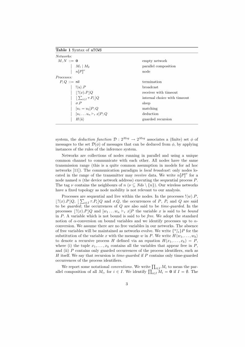
Table 1 Syntax of aTCWSNetworks:M, N ::= 0 empty network˛

M1 | M2 parallel composition˛n[P ]ν node

Processes:P, Q ::= nil termination˛

!〈u〉.P broadcast˛b?(x).P cQ receiver with timeout˛ ¨ P

i∈I τ.Pi

˝Q internal choice with timeout˛

σ.P sleep˛[u1 = u2]P ; Q matching˛[u1 . . . un `r x]P ; Q deduction˛H〈u〉 guarded recursion

system, the deduction function D : 2Msg → 2Msg associates a (finite) set φ ofmessages to the set D(φ) of messages that can be deduced from φ, by applyinginstances of the rules of the inference system.

Networks are collections of nodes running in parallel and using a uniquecommon channel to communicate with each other. All nodes have the sametransmission range (this is a quite common assumption in models for ad hocnetworks [11]). The communication paradigm is local broadcast : only nodes lo-cated in the range of the transmitter may receive data. We write n[P ]ν for anode named n (the device network address) executing the sequential process P .The tag ν contains the neighbours of n (ν ⊆ Nds \ n). Our wireless networkshave a fixed topology as node mobility is not relevant to our analysis.

Processes are sequential and live within the nodes. In the processes !〈w〉.P ,b?(x).P cQ,

⌊ ∑i∈I τ.Pi

⌋Q and σ.Q, the occurrences of P , Pi and Q are said

to be guarded ; the occurrences of Q are also said to be time-guarded. In theprocesses b?(x).P cQ and [w1 . . . wn `r x]P the variable x is said to be boundin P . A variable which is not bound is said to be free. We adopt the standardnotion of α-conversion on bound variables and we identify processes up to α-conversion. We assume there are no free variables in our networks. The absenceof free variables will be maintained as networks evolve. We write w/xP for thesubstitution of the variable x with the message w in P . We write H〈w1, . . . , wk〉to denote a recursive process H defined via an equation H(x1, . . . , xk) = P ,where (i) the tuple x1, . . . , xk contains all the variables that appear free in P ,and (ii) P contains only guarded occurrences of the process identifiers, such asH itself. We say that recursion is time-guarded if P contains only time-guardedoccurrences of the process identifiers.

We report some notational conventions. We write∏

i∈I Mi to mean the par-allel composition of all Mi, for i ∈ I. We identify

∏i∈I Mi = 0 if I = ∅. The

3

Table 2 LTS - Transmissions, internal actions and time passing

(Snd)−

m[!〈w〉.P ]νm!wBν−−−−−−→ m[P ]ν

(Rcv)m ∈ ν

n[b?(x).P cQ]νm?w−−−−→ n[w/xP ]ν

(RcvEnb)m /∈ nds (M)

Mm?w−−−−→ M

(RcvPar)M

m?w−−−−→ M ′ Nm?w−−−−→ N ′

M | Nm?w−−−−→ M ′ | N ′

(Bcast)M

m!wBν−−−−−−→ M ′ Nm?w−−−−→ N ′ µ := ν\nds (N)

M | Nm!wBµ−−−−−−→ M ′ | N ′

(Tau)h ∈ I

m[¨ P

i∈I τ.Pi

˝Q]ν

τ−−→ m[Ph]ν (TauPar)

Mτ−−→ M ′

M | Nτ−−→ M ′ | N

(σ-nil)−

n[nil]νσ−−→ n[nil]ν

(Sleep)−

n[σ.P ]νσ−−→ n[P ]ν

(σ-Rcv)−

n[b?(x).P cQ]νσ−−→ n[Q]ν

(σ-Sum)−

m[¨ P

i∈I τ.Pi

˝Q]ν

σ−−→ m[Q]ν

(σ-Par)M

σ−−→ M ′ Nσ−−→ N ′

M | Nσ−−→ M ′ | N ′ (σ-0)

−0

σ−−→ 0

process [w1 = w2]P is an abbreviation for [w1 = w2]P ; nil. Similarly, we willwrite [w1 . . . wn `r x]P to mean [w1 . . . wn `r x]P ; nil.

In the sequel, we will make use of a standard notion of structural congruenceto abstract over processes that differ for minor syntactic differences.

Definition 1. Structural congruence over networks, written ≡, is defined asthe smallest equivalence relation, preserved by parallel composition, which is acommutative monoid with respect to parallel composition and internal choice,and for which n[H〈w〉]ν ≡ n[w/xP ]ν , if H(x) = P .

Here, we provide some definitions that will be useful in the remainder of thepaper. Given a network M , nds (M) returns the node names of M . More formally,nds (0) = ∅, nds (n[P ]ν) = n and nds (M1 | M2) = nds (M1) ∪ nds (M2). Form ∈ nds (M), the function ngh(m,M) returns the set of the neighbours of min M . Thus, if M ≡ m[P ]ν | N then ngh(m,M) = ν. We write Env (M) tomean all the nodes of the environment reachable by the network M . Formally,Env (M) = ∪m∈nds(M)ngh(m,M) \ nds (M).

The syntax provided in Table 1 allows us to derive networks which are some-how ill-formed. The following definition identifies well-formed networks.

Definition 2 (Well-formedness). M is said to be well-formed if (i) M ≡ N |m1[P1]

ν1 | m2[P2]ν2 implies m1 6= m2; (ii) M ≡ N | m1[P1]

ν1 | m2[P2]ν2 , with

m1 ∈ ν2, implies m2 ∈ ν1; (iii) for all m,n ∈ nds (M) there are m1, . . . ,mk ∈nds (M), such that m=m1, n=mk, mi ∈ ngh(mi+1,M), for 1 ≤ i ≤ k−1.

In Table 2, we provide a labelled transition system (LTS) for aTCWS in theSOS style of Plotkin. Intuitively, the computation proceeds in lock-steps: between

4

Table 3 LTS - Matching, recursion and deduction

(Then)n[P ]ν

λ−−→ n[P ′]ν

n[[w = w]P ; Q]νλ−−→ n[P ′]ν

(Else)n[Q]ν

λ−−→ n[Q′]ν w1 6= w2

n[[w1 = w2]P ; Q]νλ−−→ n[Q′]ν

(Rec)n[w/xP ]ν

λ−−→ n[P ′]ν H(x)def= P

n[H〈w〉]ν λ−−→ n[P ′]ν

(DT)n[w/xP ]ν

λ−−→ n[R]ν w1. . .wn `r w

n[[w1 . . . wn `r x]P ; Q]νλ−−→ n[R]ν

(DF)n[Q]ν

λ−−→ n[R]ν 6 ∃ w. w1. . .wn `r w

n[[w1. . .wn `r x]P ; Q]νλ−−→ n[R]ν

every global synchronisation all nodes proceeds asynchronously by performingactions with no duration, which represent either broadcast or input or internalactions. Communication proceeds even if there are no listeners: Transmission is anon-blocking action. Moreover, communication is lossy as some receivers withinthe range of the transmitter might not receive the message. This may be due toseveral reasons such as signal interferences or the presence of obstacles.

The metavariable λ ranges over the set of labels τ, σ,m!wBν, m?w denotinginternal action, time passing, broadcasting and reception. Let us comment on thetransition rules of Table 2. In rule (Snd) a sender m dispatches a message w to itsneighbours ν, and then continues as P . In rule (Rcv) a receiver n gets a messagew coming from a neighbour node m, and then evolves into process P , where allthe occurrences of the variable x are replaced with w. If no message is received inthe current time slot, a timeout fires and the node n will continue with process Q,according to the rule (σ-Rcv). The rule (RcvPar) models the composition of twonetworks receiving the same message from the same transmitter. Rule (RcvEnb)

says that every node can synchronise with an external transmitter m. Noticethat a node n[b?(x).P cQ]ν might execute rule (RcvEnb) instead of rule (Rcv).This is because a potential receiver may miss a message for several reasons(internal misbehaving, interferences, weak radio signal, etc); in this manner wemodel message loss. Rule (Bcast) models the propagation of messages on thebroadcast channel. Note that this rule looses track of the neighbours of m thatare in N . Thus, in the label m!wBν the set ν always contains the neighboursof m which can receive the message w. The remaining rules are straightforward.Rules (Bcast) and (TauPar) have their symmetric counterparts. Table 3 reportsthe standard rules for nodes containing matching, recursion or deduction.

Below, we report a number of basic properties of our LTS.Proposition 1. Let M , M1 and M2 be well-formed networks.

1. m 6∈ nds (M) if and only if Mm?w−−−−→ N , for some network N .

2. M1 | M2m?w−−−−→ N if and only if there are N1 and N2 such that M1

m?w−−−−→N1, M2

m?w−−−−→ N2 with N = N1 | N2.

3. If Mm!wBµ−−−−−−→ M ′ then M ≡ m[!〈w〉.P ]ν | N , for some m, ν, P and N

such that m[!〈w〉.P ]νm!wBν−−−−−−→ m[P ]ν , N

m?w−−−−→ N ′, M ′ ≡ m[P ]ν | N ′ andµ = ν \ nds (N).

5

4. If Mτ−−→ M ′ then M ≡ m[

⌊ ∑i∈I τ.Pi

⌋Q]ν | N , for some m, ν, Pi, Q and

N such that m[⌊ ∑

i∈I τ.Pi

⌋Q]ν

τ−−→ m[Ph]ν , for some h ∈ I, and M ′ ≡

m[Ph]ν | N .

5. M1 | M2σ−−→ N if and only if there are N1 and N2 such that M1

σ−−→ N1,M2

σ−−→ N2 and N = N1 | N2.

Proposition 2. Let M be well-formed. If Mλ−−→ M ′ then M ′ is well-formed.

Based on the LTS of Section 2, we define a standard notion of timed labelledsimilarity for aTCWS. We distinguish between the transmissions which may beobserved and those which may not be observed by the environment. We extendthe set of rules of Table 2 with the following two rules:

(Shh)M

m!wB∅−−−−−−→ M ′

Mτ−−→ M ′

(Obs)M

m!wBν−−−−−−→ M ′ µ ⊆ ν µ 6= ∅M

!wBµ−−−−−→ M ′

Rule (Shh) models transmissions that cannot be observed because none of thepotential receivers is in the environment. Rule (Obs) models transmissions thatcan be received (and hence observed) by those nodes of the environment con-tained in ν. Notice that the name of the transmitter is removed from the label.This is motivated by the fact that nodes may refuse to reveal their identities, e.g.for security reasons or limited sensory capabilities in perceiving these identities.

In the sequel, the metavariable α will range over the following actions: τ ,σ, !wBν and m?w. We adopt the standard notation for weak transitions: therelation =⇒ denotes the reflexive and transitive closure of

τ−−→; the relation α==⇒denotes =⇒ α−−→ =⇒; the relation α==⇒ denotes =⇒ if α = τ and α==⇒ otherwise.

Definition 3 (Similarity). A relation R over well-formed networks is a sim-ulation if M R N and M

α−−→ M ′ imply there is N ′ such that Nα==⇒ N ′ and

M ′ R N ′. We write M . N , if there is a simulation R such that M R N .

Our notion of of similarity between networks is a pre-congruences, as it is pre-served by parallel composition.

Theorem 1. Let M and N be two well-formed networks such that M . N .Then M | O . N | O for all O such that M | O and N | O are well-formed.

3 A tGNDC schema for Wireless Networks

Gorrieri and Martinelli [5] have proposed a general schema for the definition oftimed security properties, called timed Generalized Non-Deducibility on Compo-sitions (tGNDC ). Basically, a system M is tGNDC ρ(M) if for any attacker A

M∣∣ A . ρ(M)

i.e. the composed system M | A satisfies the abstraction ρ(M).

6

A wireless protocol involves a set of nodes which may be potentially underattack, depending on the proximity to the attacker. This means that, in general,the attacker of a protocol M is a distinct network A of possibly colluding nodes.For the sake of compositionality, we assume that each node of the protocol isattacked by exactly one node of A.

Definition 4. We say that A is a set of attacking nodes for the network M ifand only if |A| = nds (M) and A ∩ (nds (M) ∪ Env (M)) = ∅.

During the execution of the protocol an attacker may increase its initial knowl-edge by grasping messages sent by the parties, according to Dolev-Yao constrains.The knowledge of a network is expressed by the set of messages that the net-work can manipulate. Thus, we write msg(M) (resp. msg(P )) to denote the setof the messages appearing in the network M (resp. in the process P ). To ensurethat attackers cannot prevent the passage of time, in the following definition wedenote Prcwt the set of processes in which summations are finite-indexed andrecursive definitions are time-guarded.

Definition 5 (Attacker). Let M be a network, with nds (M) =m1, ...,mk.Let A = a1, . . . , ak be a set of attacking nodes for M . We define the set ofattackers of M with initial knowledge φ0 ⊆ Msg as:

Aφ0A/M

def= k∏

i=1

ai[Qi]µi : Qi ∈ Prcwt, msg(Qi) ⊆ D(φ0), µi=(A \ ai) ∪mi

.

Sometimes, for verification reasons, we will be interested in observing partof the protocol M under examination. For this purpose, we assume that theenvironment contains a fresh node obs /∈ nds (M) ∪ Env (M) ∪ A, that we callthe ‘observer’, unknown to the attacker. For convenience, the observer cannottransmit: it can only receive messages.

Definition 6. Let M=∏k

i=1 mi[Pi]νi . Given a set A=a1, . . . , ak of attacking

nodes for M and fixed a set O ⊆ nds (M) of nodes to be observed, we define:

MAO

def=k∏

i=1

mi[Pi]ν′i where ν′i

def=

(νi ∩ nds (M)) ∪ ai ∪ obs if mi ∈ O(νi ∩ nds (M)) ∪ ai otherwise.

This definition expresses that (i) every node mi of the protocols has a dedicatedattacker located at ai, (ii) network and attacker are considered in isolation,without any external interference, (iii) only obs can observe the behaviour ofnodes in O, (iv) node obs does not interfere with the protocol as it cannottransmit, (v) the behaviour of the nodes in nds (M) \ O is not observable.

We can now formalise the tGNDC family properties as follows.

Definition 7 (tGNDC for wireless networks). Given a network M , an ini-tial knowledge φ0, a set O ⊆ nds (M) of nodes under observation and an abstrac-tion ρ(M), representing a security property for M , we write M ∈ tGNDC ρ(M)

φ0,O

if and only if for all sets A of attacking nodes for M and for every A ∈ Aφ0A/M

it holds that MAO

∣∣ A . ρ(M).

7

It should be noticed that when showing that a system M is tGNDC ρ(M)φ0,O , the

universal quantification on attackers required by the definition makes the proofquite involved. Thus, we look for a sufficient condition which does not make useof the universal quantification. For this purpose, we rely on a timed notion ofterm stability [5]. Intuitively, a network M is said to be time-dependent stable ifthe attacker cannot increase its knowledge in a indefinite way when M runs inthe space of a time slot. Thus, we can predict how the knowledge of the attackerevolves at each time slot. First, we need a formalisation of computation. ForΛ=α1 . . . αn, we write Λ==⇒ to denote =⇒ α1−−−→ =⇒ ... =⇒ αn−−−→ =⇒. In order tocount how many time slots embraces an execution trace Λ, we define #σ(Λ) tobe the number of occurrences of σ-actions in Λ.

Definition 8 (Time-dependent stability). A network M is said to be time-dependent stable with respect to a sequence of knowledge φjj≥0 if whenever

MAnds(M)

∣∣A Λ==⇒ M ′∣∣A′, where A is a set of attacking nodes for M , #σ(Λ) = j,

A ∈ Aφ0A/M and nds (M ′) = nds (M), then msg(A′) ⊆ D(φj).

The set of messages φj expresses the knowledge of the attacker at the end ofthe j-th time slot. Time-dependent stability is the crucial notion that allows usto introduce the notion of most general attacker. Intuitively, given a sequenceof knowledge φjj≥0 and a network M , with P = nds (M), we pick a set A =a1, . . . , ak of attacking nodes for M and we define the top attacker Top

φj

A/Pas the network which at (the beginning of) the j-th time slot is aware of theknowledge (derivable) from φj .

Definition 9 (Top Attacker). Let M be a network with P=nds (M) =⋃k

i=1 mi.Let A = a1, . . . , ak be a set of attacking nodes for M , and φjj≥0 a sequenceof knowledge. We define:

Topφj

A/Pdef=

∏ki=1 ai[Tφj

]mi where Tφj

def=⌊ ∑

w∈D(φj)τ.!〈w〉.Tφj

⌋Tφj+1 .

Basically, from j-th time slot onwards, Topφj

A/P can replay any message in D(φj)to the network under attack. Moreover, every attacking node ai can send mes-sages to the corresponding node mi, but, unlike the attackers of Definition 5, itdoes not need to communicate with the other nodes in A as it already owns thefull knowledge of the system at time j.

Top attackers are strong enough to guarantee tGNDC.Theorem 2 (Criterion for tGNDC ). Let M be time-dependent stable withrespect to a sequence φjj≥0, A be a set of attacking nodes for M and O ⊆nds (M) = P. Then MA

O∣∣ Topφ0

A/P . N implies M ∈ tGNDCNφ0,O.

Top attackers can be employed to reason in a compositional manner.Theorem 3 (Compositionality). Let M = M1 | . . . | Mk be time-dependentstable with respect to a sequence of knowledge φjj≥0. Let A1, . . . ,Ak be disjointsets of attacking nodes for M1, . . . ,Mk, respectively. Let Oi ⊆ nds (Mi) = Pi,for 1 ≤ i ≤ k. Then, (Mi)Ai

Oi

∣∣ Topφ0Ai/Pi

. Ni, for 1 ≤ i ≤ k, implies M ∈tGNDC N1|...|Nk

φ0,O1∪...∪Ok.

8

4 A security analysis of LiSP

LiSP [13] is a well-known key management protocol for wireless sensor net-works. A LiSP network consists of a Key Server (ks) and a set of sensor nodesm1, . . . ,mk. The protocol assumes a one way function F , pre-loaded in everynode of the system, and employs two different key families: (i) a set of temporalkeys k0, . . . , kn, computed by ks by means of F , and used by all nodes to en-crypt/decrypt data packets; (ii) a set of master keys kks:mj , one for each nodemj , for unicast communications between mj and bs. The transmission time issplit into time intervals, each of them is ∆refresh time units long. Thus, eachtemporal key is tied to a time interval and renewed every ∆refresh time units.At a time interval i, the temporal key ki is shared by all sensor nodes and it isused for data encryption. Key renewal relies on loose node time synchronisationamong nodes. Each node stores a subset of temporal keys in a buffer of a fixedsize, say s with s << n.

The LiSP protocol consists of the following phases.

Initial Setup. At the beginning, ks randomly chooses a key kn and computesa sequence of temporal keys k0, . . . , kn, by using the function F , as ki :=F (ki+1). Then, ks waits for reconfiguration requests from nodes. More pre-cisely, when ks receives a reconfiguration request from a node mj , at timeinterval i, it unicasts the packet InitKey:

ks → mj : enc(kks:mj , (s | ks+i | ∆refresh)) | hash(s | ks+i | ∆refresh) .

The operator enc(k, p) represents the encryption of p by using the key of k,while hash(p) generates a message digest for p by means of a cryptographichash function used to check the integrity of the packet p. When mj receivesthe InitKey packet, it computes the sequence of keys ks+i−1, ks+i−2, . . . , ki

by several applications of the function F to ks+i. Then, it activates ki fordata encryption and it stores the remaining keys in its local buffer; finallyit sets up a ReKeyingTimer to expires after ∆refresh/2 time units (this valueapplies only for the first rekeying).

Re-Keying. At each time interval i, with i ≤ n, ks employs the active encryp-tion key ki to encode the key ks+i. The resulting packet is broadcast as anUpdateKey packet:

ks → ∗ : enc(ki, ks+i) .

When a node receives an UpdateKey packet, it tries to authenticate the keyreceived in the packet; if the node succeeds in the authentication then itrecovers all keys that have been possibly lost and updates its key buffer.When the time interval i elapses, every node discards ki, activates the keyki+1 for data encryption, and sets up the ReKeyingTimer to expire after∆refresh time units for future key switching (after the first time, switchinghappens every ∆refresh time units).

Authentication and Recovery of Lost Keys. The one-way function F is used toauthenticate and recover lost keys. If l is the number of stored keys in a buffer

9

of size s, with l ≤ s, then s−l represents the number of keys which have beenlost by the node. When a sensor node receives an UpdateKey packet carryinga new key k, it calculates F s−l(k) by applying s− l times the function F . Ifthe result matches with the last received temporal key, then the node storesk in its buffer and recovers all lost keys.

Reconfiguration. When a node mj joins the network or misses more than s tem-poral keys, then its buffer is empty. Thus, it sends a RequestKey packet inorder to request the current configuration:

mj → ks : RequestKey | mj .

Upon reception, node ks performs authentication of mj and, if successful, itsends the current configuration via an InitKey packet.

Encoding In Table 4, we provide a specification in aTCWS of the entire LiSPprotocol. We introduce some slight simplifications with respect to the originalprotocol. We assume that (i) the temporal keys k0, . . . , kn have already beencomputed by ks, (ii) both the buffer size s and the refresh interval ∆refresh areknown by each node. Thus, the InitKey packet can be simplified as follows:

ks → mj : enc(kks:mj , ks+i) | hash(ks+i) .

Moreover, we assume that every σ-action models the passage of ∆refresh/2 timeunits. Therefore, every two σ-actions the key server broadcasts the new temporalkey encrypted with the key tied to that specific interval. Finally, we do not modeldata encryption.

When giving our encoding in aTCWS we will require some new deduction rulesto model an hash function and encryption/decryption of messages:

(hash)w

hash(w)(enc)

w1 w2

enc(w1, w2)(dec)

w1 w2

dec(w1, w2).

The protocol executed by the key server is expressed by the following twothreads: a key distributor Di and a listener Li waiting for reconfiguration re-quests from the sensor nodes, with i being the current time interval. Every∆refresh time units (that is, every two σ-actions) Di broadcasts the new tempo-ral key ks+i encrypted with the key ki of the current time interval i. The processLi replies to reconfiguration requests by sending an initialisation packet.

At the beginning of the protocol, a sensor node runs the process Z, whichbroadcasts a request packet to ks, waits for a reconfiguration packet q, and thenchecks authenticity by verifying the hash code. If the verification is successfulthen the node starts the broadcasting new keys phase. This phase is formalisedby the process R(kc, kl, l), where kc is the current temporal key, kl is the lastauthenticated temporal key, and the integer l counts the number of keys thatare actually stored in the buffer.

To simplify the exposition, we formalise the key server as a pair of nodes: akey disposer kd, which executes Di, and a listener kl, which executes Li. Thus,

10

Table 4 The LiSP protocolKey Server:

D0def= σ.D1 synchronise and move to D1

Didef= [ki ks+i `enc ti] for i ≥ 1, encrypt ks+i with ki

[UpdateKey ti `pair ui] build the UpdateKey packet ui

!〈ui〉.σ.σ.Di+1 broadcast ri, and move to Di+1

Lidef= b?(r).Ii+1cσ.Li+1 wait for request packets

Iidef= [r `fst r1]I

1i ; σ.σ.Li extract first component

I1i

def= [r1 = RequestKey]I2

i ; σ.σ.Li check if r1 is a RequestKey

I2i

def= [r `snd m] extract node name

[kks:m ks+i `enc wi] encrypt ks+i with kks:m

[ks+i `hash hi] calculate hash code for ks+i

[wi hi `pair ri] build a pair ri,[InitKey ri `pair qi] build a InitKey packet qi,σ.!〈qi〉.σ.Li broadcast qi, move to Li

Receiver at node m:

Zdef= [RequestKey m `pair r] send a RequestKey packet

!〈r〉.σ.b?(q).T cZ wait for a reconfig. packet

Tdef= [q `fst q′]T 1; σ.Z extract fst component of q

T 1 def= [q′ = InitKey]T 2; σ.Z check if q is a InitKey packet

T 2 def= [q `snd q′′] extract snd component of q

[q′′ `fst w]T 3; σ.Z extract fst component of q′′

T 3 def= [q′′ `snd h] extract snd component of q′′

[kks:m w `dec k]T 3; σ.Z extract the key

T 4 def= [k `hash h′][h = h′]T 5; σ.Z verify hash codes

T 5 def= σ.σ.R〈F s−1(k), k, s−1〉 synchronise and move to R

R(kc, kl, l)def= b?(u).EcF wait for incoming packets

Edef= [u `fst u′]E1; σ.F extract fst component of u

E1 def= [u′ = UpdateKey]E2; σ.F check UpdateKey packet

E2 def= [u `snd u′′] extract snd component of u

[kc u′′ `dec k]E3; σ.F decrypt u′′ by using kc

E3 def= [F s−l(k) = kl]E

4; σ.F authenticate k

E4 def= σ.σ.R〈F s−1(k), k, s−1〉 synchronise and move to R

Fdef= [l = 0]Z; σ.R〈F l−1(kl), kl, l−1〉 check if buffer key is empty

the LiSP protocol, in its initial configuration, can be represented as:

LiSP def=∏j∈J

mj[σ.Z]νmj | ks[σ.D0]νks | kl[σ.L0]

νkl

where for each node mj , with j ∈ J , mj ∈ νkd ∩ νkl and kd,kl ⊆ νmj.

11

Security Analysis In LiSP, a node should authenticate only keys sent by thekey server in the previous ∆refresh time units. Otherwise, a node needing a re-configuration would authenticate an obsolete temporal key and it would not besynchronised with the rest of the network. Here, we show that key authenticationmay take longer than ∆refresh time units, as a consequence of an attack.

For our analysis, without loss of generality, it suffices to focus on a part of theprotocol composed by the kl node of the key server and a single sensor node m.Moreover, in order to make observable a successful reconfiguration, we replacethe process T 4 of Table 4 with the process

T 4′ def= σ.σ.[auth k `pair a]!〈a〉.R〈F s−1(k), k, s−1〉 .

Thus, the part of the protocol under examination can be defined as follows:

LiSP′ def= m[σ.Z ′]νm | kl[σ.L0]νkl .

Our freshness requirement on authenticated keys can be expressed by the fol-lowing abstraction of the protocol:

ρ(LiSP′) def= m[σ.Z0]obs | kl[σ.L0]

obs

where

– Zidef= !〈r〉.σ.

⌊τ.σ.σ.!〈authi+1〉.R(ki+1, ks+i, s− 1)

⌋Zi+1,

with r = pair(RequestKey, m) and authi = pair(auth, ks+i) as in Table 4;– Li

def=⌊τ.σ.!〈qi+1〉.σ.Li+1

⌋σ.Li+1, and qi defined as in Table 4:

qi = pair(InitKey ri) with ri = pair(enc(kks:m, ks+i),hash(ks+i)).

It is easy to see that ρ(LiSP′) is a correct abstraction of key authenticationwithin the protocol, as the action authi occurs exactly ∆refresh time units (thatis, two σ-actions) after the disclosure of key ks+i through packet qi.

Proposition 3. ρ(LiSP′) Λ==⇒ !qiBobs−−−−−−−→ Ω==⇒ !authiBobs−−−−−−−−−→ implies #σ(Ω) = 2.

In order to show that LiSP′ satisfies our security analysis, we should prove that

LiSP′ ∈ tGNDC ρ(LiSP′)φ0,O

for O = nds(LiSP′

)and initial knowledge φ0 = ∅. However, this is not the case.

Theorem 4 (Replay attack to LiSP).

LiSP′ 6∈ tGNDC ρ(LiSP′)∅,kl,m .

Proof Let us define the set of attacking nodes A = a, b for LiSP′. Letus fix the initial knowledge of the attacker φ0 = ∅. We set νa = m, b andνb = kl, a, and we assume that O = kl,m. We give an intuition of thereplay attack in Table 5. Basically, an attacker may prevent the node m toreceive the InitKey packet within ∆refresh time units. As a consequence, m may

12

Table 5 Replay attack to LiSP

m −→ kl : r m sends a RequestKey and kl correctly receives the packetσ−−→ the system moves to the next time slot

kl −→ m : q1 kl replies with an InitKey which is lost by m and grasped by bσ−−→ the system moves to the next time slot

b → a : q1 b sends q1 to am → kl : r m sends a new RequestKey which gets lost

σ−−→ the system moves to the next time slota → m : q1 a replays q1 to m

σ−−→ σ−−→ after ∆refresh time unitsm → ∗ : auth1 m authenticates q1 and signals the end of the protocol

complete the protocol only after 2∆refresh time units (that is, four σ-actions),so authenticating an old key. Formally, we define the attacker A ∈ Aφ0

A/kl,m asA = a[σ.σ.σ.X]νa

∣∣ b[σ.σ.X]νb where X = b?(x).σ.!〈x〉.nilcnil. We then considerthe system (LiSP′)AO | A which admits the following execution trace:

σ . !rBobs . σ . !q1Bobs . σ . τ . !rBobs . σ . τ . σ . σ . !auth1Bobs

containing four σ-actions between the packets q1 and auth1. By Proposition 3,this trace cannot be matched by ρ(LiSP′). So, (LiSP′)AO | A 6. ρ(LiSP′).

4.1 LiSP with nonces

Replay attacks as those described above appears also in other key managementprotocols, such as µTESLA [14] and LEAP+ [17]. These protocols have beenamended by adding nonces to guarantee freshness. We propose to do the samein LiSP. For this purpose, we extend our inference system with a new deductionrule to model a pseudo-random function: The application prf(m,wi) returns apseudo-random value wi+1 associated to a node m and the last generated valuewi. In our amended specification of LiSP, we add a nonce to the RequestKeypacket. The nonce is then included in the corresponding InitKey packet to guar-antee the freshness of the reply. These changes affect only those processes whichmodel the key request at the node side and the reply at the server side. We mod-ify these processes as shown in Table 6. The requesting nodes run the processZj , where j is the number associated to the current key request. At each requestj, the receiver generates a nonce nj which will be used to check the freshnessof the received key. The process Li, running at the key server, now includes thereceived nonce in the InitKey packet. Notice that, as done before, the process T 7

j

signals a successful reconfiguration. Again, for our analysis, it suffices to analysethe following fragment of the protocol:

LiSP′′ def= m[σ.Z1]νm | kl[σ.L0]

νkl .

13

Table 6 LiSP with noncesKey Server:

Lidef= b?(r).Ii+1cσ.Li+1 wait for request packets

Iidef= [r `fst r1]I

1i ; σ.σ.Li+1 extract first component

I1i

def= [r1 = RequestKey]I2

i ; σ.σ.Li+1 check if r1 is a RequestKey

I2i

def= [r `snd t] extract second component

[t `fst m]I3i ; σ.σ.Li+1 extract node name

I3i

def= [t `snd n] extract nonce

[ks+i n `pair p] build a pair[kks:m p `enc wi] encrypt p with kks:m

[ks+i `hash hi] calculate hash code for ks+i

[wi hi `pair ri] build a pair ri,[InitKey ri `pair qi] build a InitKey packet qi,σ.!〈qi〉.σ.Li+1 broadcast qi, move to Li+1

Receiver at node m:

Zjdef= [m nj−1 `prf nj ] build a random nonce nj

[m nj `pair t] build a pair t with name m and nonce nj

[RequestKey t `pair r] send a RequestKey packet!〈r〉.σ.b?(q).TjcZj+1 wait for a reconfig. packet

Tjdef= [q `fst q′]T 1

j ; σ.Zj+1 extract fst component of q

T 1j

def= [q′ = InitKey]T 2

j ; σ.Zj+1 check if q is a InitKey packet

T 2j

def= [q `snd q′′] extract snd component of q

[q′′ `fst w]T 3j ; σ.Zj+1 extract fst component of q′′

T 3j

def= [q′′ `snd h] extract snd component of q′′

[kks:m w `dec p]T 4j ; σ.Zj+1 decript w

T 4j

def= [p `fst k]T 5

j ; σ.Zj+1 extract the key

T 5j

def= [p `snd n][n = nj ]T

6j ; σ.Zj+1 verify nonces

T 6j

def= [k `hash h′][h = h′]T 7

j ; σ.Zj+1 verify hash codes

T 7j

def= σ.σ.[auth k `pair a]!〈a〉.nil reaching of synchronisation

According to Definition 8, the system LiSP′′ is time-dependent stable with re-spect to the following sequence of knowledge:

φ0def= ∅

φ1def= r1

φidef= φi−1 ∪ qj if j > 0 and i = 2j

φidef= φi−1 ∪ authj , rj+1 if j > 0 and i = 2j + 1

(1)

where

authj = pair(auth, ks+j)rj = pair(RequestKey,pair(m,nj))qj = pair( InitKey, pair( enc(kks:m,pair(ks+j , nj)), hash(ks+j) ) ) .

14

Intuitively, φi consists of φi−1 together with the set of messages an intruder canget by eavesdropping on a run of the protocol during the time slot i.

With the introduction of nonces, the abstraction expressing key authentica-tion within ∆refresh time units becomes the following:

ρ(LiSP′′) def= m[σ.Z ′1]

obs | kl[σ.L′0]obs

where

– Z ′i

def= [m ni−1 `prf ni][m ni `pair t][RequestKey t `pair r]!〈r〉.σ.⌊τ.σ.σ.!〈authi+1〉.nil

⌋Z ′

i+1

– L′idef=

⌊ ∑v∈D(φ2i+1)

τ.σ.!〈qvi+1〉.σ.L′i+1

⌋σ.L′i+1

with qvi = pair(InitKey pair(enc(kks:m,pair(ks+i, v)),hash(ks+i))).

In ρ(LiSP′′) keys are authenticated after ∆refresh time units (two σ-actions).

Proposition 4. ρ(LiSP′′) Λ==⇒!qv

i Bobs−−−−−−−→ Ω==⇒ !authiBobs−−−−−−−−−→ M implies #σ(Ω)=2.

Now, everything is in place to prove the safety of the LiSP protocol with nonces.

Lemma 1. Given two attacking nodes a and b, for m and kl respectively, andfixed the sequence of knowledge φii≥0 as in (1), then

1. kl[σ.L0]b,obs ∣∣ Topφ0

b/kl . kl[σ.L′0]obs

2. m[σ.Z1]a,obs ∣∣ Topφ0

a/m . m[σ.Z ′1]

obs .

Theorem 5 (Safety of LiSP with nonces). LiSP′′ ∈ tGNDC ρ(LiSP′′)∅,nds(LiSP′′) .

Proof By an application of Lemma 1 and Theorem 3.

References

1. Ballardin, F., Merro, M.: A calculus for the analysis of wireless network securityprotocols. In: FAST. LCNS, vol. 6561, pp. 206–222. Springer (2010)

2. Ghassemi, F., Fokkink, W., Movaghar, A.: Equational Reasoning on Mobile AdHoc Networks. Fundamentae Informaticae 105(4):375–415 (2010)

3. Godskesen, J.C.: A Calculus for Mobile Ad Hoc Networks. In: COORDINATION.LNCS, vol. 4467, pp. 132–150. Springer (2007)

4. Godskesen, J.C., Nanz, S.: Mobility Models and Behavioural Equivalence for Wire-less Networks. In:COORDINATION. LNCS, vol.5521, pp.106–122. Springer (2009)

5. Gorrieri, R., Martinelli, F.: A simple framework for real-time cryptographic proto-col analysis with compositional proof rules. Sc. of Com. Prog. 50, 23–49 (2004)

6. Gorrieri, R., Martinelli, F., Petrocchi, M.: Formal models and analysis of securemulticast in wired and wireless networks. J. Aut. Reasoning 41(3-4), 325–364 (2008)

7. Hennessy, M., Regan, T.: A Process Algebra for Timed Systems. Information andComputation 117(2), 221–239 (1995)

8. Lanese, I., Sangiorgi, D.: An Operational Semantics for a Calculus for WirelessSystems. Theoretical Computer Science 411, 1928–1948 (2010)

9. Merro, M.: An Observational Theory for Mobile Ad Hoc Networks (full paper).Information and Computation 207(2), 194–208 (2009)

15

10. Merro, M., Ballardin, F., Sibilio, E.: A Timed Calculus for Wireless Systems. The-oretical Computer Science 412(47), 6585–6611 (2011)

11. Misra, S., Woungag, I.: Guide to Wireless Ad Hoc Networks. Computer Commu-nications and Networks, Springer (2009)

12. Nanz, S., Hankin, C.: A Framework for Security Analysis of Mobile Wireless Net-works. Theoretical Computer Science 367(1-2), 203–227 (2006)

13. Park, T., Shin, K.G.: LiSP: A lightweight security protocol for wireless sensornetworks. ACM Trans. Embedded Comput. Syst. 3(3), 634–660 (2004)

14. Perrig, A., Szewczyk, R., Tygar, J.D., Wen, V., Culler, D.: SPINS: Security Pro-tocols for Sensor Networks. Wireless Networks 8(5), 521–534 (2002)

15. Singh, A., Ramakrishnan, C.R., Smolka, S.A.: A Process Calculus for Mobile AdHoc Networks. In: COORDINATION. LNCS, vol. 5052, pp. 296–314. (2008)

16. Sundararaman, B., Buy, U., Kshemkalyani, A.D.: Clock synchronization for wire-less sensor networks: a survey. Ad Hoc Networks 3(3), 281–323 (2005)

17. Zhu, S., Setia, S., Jajodia, S.: Leap+: Efficient security mechanisms for large-scaledistributed sensor networks. ACM Trans. on Sensor Networks 2(4), 500–528 (2006)

A Appendix

A.1 Proofs of Section 2Proof of Proposition 1 We single out each item of the proposition.Item 1. The forward direction is an instance of rule (RcvEnb), the converse isproved by a straightforward rule induction.Item 2. The forward direction follows by noticing that only rules (RcvEnb) and(RcvPar) are suitable for deriving the action m?w from M1 | M2; in the case ofrule (RcvEnb) we just apply rule (RcvEnb) both on M1 and on M2, in the case ofrule (RcvPar) the premises require both M1 and M2 to perform an action m?wand to move to N1 and N2 with N = N1 | N2. The converse is an instance ofrule (σ-Par).Item 3. The result is a consequence of the combination of rules (Snd) and (Bcast)

and it is proved by a straightforward rule induction.Item 4. Again, the proof is done by a straightforward rule induction.Item 5. The forward direction follows by noticing that the only rule for derivingthe action σ from M1 | M2 is (σ-Par) which, in the premises, requires both M1

and M2 to perform an action σ. The converse is an instance of rule (σ-Par).

Proof of Proposition 2 The property is a consequence of the fact that thetopology of networks is static.

A.2 Time properties

Our calculus aTCWS enjoys some desirable time properties. Here, we outline themost significant ones. Proposition 5 formalises the deterministic nature of timepassing: a network can reach at most one new state by executing a σ-action.

Proposition 5 (Time Determinism). If M is a well-formed network withM

σ−−→ M ′ and Mσ−−→ M ′′, then M ′ and M ′′ are syntactically the same.

Proof By induction on the length of the proof of Mσ−−→ M ′.

16

Patience guarantees that a process will wait indefinitely until it can commu-nicate [7]. In our setting, this means that

Proposition 6 (Patience). Let M ≡∏

i∈I mi[Pi]νi be a well-formed network,

such that for all i ∈ I it holds that mi[Pi]νi 6≡ mi[!〈w〉.Qi]

νi , then there is anetwork N such that M

σ−−→ N .Proof By induction on the structure of M .

The maximal progress property says that processes communicate as soon asa possibility of communication arises [7]. In other words, the passage of timecannot block transmissions.

Proposition 7 (Maximal Progress). Let M be a well-formed network. IfM ≡ m[!〈w〉.P ]ν | N then M

σ−−→ M ′ for no network M ′.

Proof By inspection on the rules that can be used to derive Mσ−−→ M ′,

because sender nodes cannot perform σ-actions.

Basically, time cannot pass unless the specification itself explicitly asks for it.This approach provides a lot of power to the specification, which can preciselyhandle the flowing of time. Such an extra expressive power leads, as a drawback,to the possibility of abuses. For instance, infinite loops of broadcast actionsor internal computations prevent time passing. The well-timedness (or finitevariability) property puts a limitation on the number of instantaneous actionsthat can fire between two contiguous σ-actions. Intuitively, well-timedness saysthat time passing never stops: Only a finite number of instantaneous actions canfire between two subsequent σ-actions.

Definition 10 (Well-Timedness). A network M satisfies well-timedness if

there exists an upper bound k ∈ N such that whenever Mλ1−−−→ · · · λh−−−→ where λj

is not directly derived by an application of (RcvEnb) and λj 6= σ (for 1 ≤ j ≤ h)then k ≤ h.

The above definition takes into account only transitions denoting an active in-volvement of the network, that is why we have left out those transitions whichcan be derived by applying rule (RcvEnb). However, as aTCWS is basically a speci-fication language, there is no harm in allowing specifications which do not respectwell-timedness. Of course, when using our language to give a protocol implemen-tation, then one must verify that the implementation satisfies well-timedness: Noreal-world service (even a attackers) can stop the passage of time.

The following proposition provides a criterion to check well-timedness. Werecall that recursion is time-guarded if P contains only time-guarded occurrencesof the process identifiers. We write Prcwt for the set of processes in which sum-mations are finite-indexed and recursive definitions are time-guarded.

Proposition 8. Let M =∏

i∈I mi[Pi]νi be a network. If for all i ∈ I we have

Pi ∈ Prcwt then M satisfies well-timedness.Proof First notice that without an application of (RcvEnb) the network Mcan perform only a finite number of transitions. Then proceed by induction onthe structure of M .

17

Remark 1. By Proposition 8, the requirement Qi ∈ Prcwt in the definition ofAφ0A/P guarantees that our attackers respects well-timedness and hence cannot

prevent the passage of time.

Remark 2. Notice that the top attacker does not satisfy well-timedness (see Def-inition 10), as the process identifiers involved in the recursive definition are nottime-guarded. However, this is not a problem as we are looking for a sufficientcondition which ensures tGNDC with respect to well-timed attackers.

A.3 Proofs of Section 2

Proposition 9. If M . N then nds (N) ⊆ nds (M).Proof By contradiction. Assume there exists a node m such that m ∈ nds (N)

and m /∈ nds (M). Then, by rule (RcvEnb), Mm?w−−−−→ M . Since M . N there

must be N ′ such that Nm?w====⇒ N ′ with M ′ . N ′. However, since m ∈ nds (N),

by inspection on the transition rules, there is no way to deduce a weak transitionof the form N

m?w====⇒ N ′.

Proof of Theorem 1 We prove that the relation

R = (

M | O, N | O)

s.t. M . N and M | O, N | O are well-formed

is a simulation. We proceed by case analysis on why M | Oα−−→ Z. The inter-

esting cases are when the transition is due to an interaction between M and O.The remaining cases are more elementary.

Let M | O!wBν−−−−−→ M ′ | O′ (ν 6= ∅) by an application of rule (Obs), because

M | O m!wBη−−−−−−→ M ′ | O′, by an application of rule (Bcast) with ν ⊆ η. There aretwo possible ways to derive this transition, depending on where the sender nodeis located in the network.

1. Mm!wBµ−−−−−−→ M ′ and O

m?w−−−−→ O′, with m ∈ nds (M) and η = µ\nds (O). By

an application of rule (Obs) we obtain that M!wBµ−−−−−→ M ′. Since M . N ,

it follows that there is N ′ such that N!wBµ

=====⇒ N ′ with M ′ . N ′. This

implies that there exists h ∈ nds (N) such that Nh!wBµ′

======⇒ N ′ with µ ⊆ µ′.Moreover:(a) h /∈ nds (O), as N | O is well-formed and it cannot contain two nodes

with the same name;(b) µ′ ⊆ ngh(h, N), by Proposition 1(3);(c) If k ∈ µ′ ∩ nds (O) then h ∈ ngh(k, O), as the neighbouring relation is

symmetric.

Now, in case Om?w−−−−→ O′ exclusively by rule (RcvEnb) then also O

h?w−−−−→ O′

by rule (RcvEnb) and item (a). In case the derivation of Om?w−−−−→ O′ involves

some applications of the rule (Rcv) then the concerned nodes have the form

18

k[b?(x).P cQ]π with k ∈ µ, hence h ∈ ngh(k, O) by item (c), and so we can

derive Oh?w−−−−→ O′ by applying the rules (RcvEnb) and (RcvPar).

Thus we have Oh?w−−−−→ O′ in any case. Then by an application of rule (Bcast)

and several applications of rule (TauPar) we have N | Oh!wBη′

======⇒ N ′ | O′

with η′ = µ′ \ nds (O). Now, since µ ⊆ µ′ we have µ \ nds (O) ⊆ µ′ \ nds (O)hence ν ⊆ η ⊆ η′. As ν 6= ∅, by an application of rule (Obs) and severalapplications of rule (TauPar) it follows that N | O

!wBν=====⇒ N ′ | O′. SinceM ′ . N ′, we obtain (M ′ | O′, N ′ | O′) ∈ R.

2. Mm?w−−−−→ M ′ and O

m!wBµ−−−−−−→ O′, with m ∈ nds (O) and η = µ \ nds (M).Since M . N , it follows that there is N ′ such that N

m?w====⇒ N ′ withM ′ . N ′. By an application of rule (Bcast) and several applications of rule

(TauPar) we have N | Om!wBη′

=======⇒ N ′ | O′, with η′ = µ \ nds (N). SinceM . N , by Proposition 9 we have η ⊆ η′. Thus ν ⊆ η′ and by an applicationof rule (Obs) and several applications of rule (TauPar) it follows that N |O

!wBν=====⇒ N ′ | O′. Since M ′ . N ′, we obtain (M ′ | O′, N ′ | O′) ∈ R.

Let M | Oτ−−→ M ′ | O′ by an application of rule (Shh) because M |

Om!wB∅−−−−−−→ M ′ | O′. This case is similar to the previous one.

Let M | Om?w−−−−→ M ′ | O′ by an application of rule (RcvPar) because

Mm?w−−−−→ M ′ and O

m?w−−−−→ O′. Since M . N , it follows that there is N ′

such that Nm?w====⇒ N ′ with M ′ . N ′. By an application of rule (RcvPar)

and several applications of rule (TauPar) we have N | Om?w====⇒ N ′ | O′. Since

M ′ . N ′, we obtain (M ′ | O′, N ′ | O′) ∈ R.Let M | O σ−−→ M ′ | O′ by an application of rule (σ-Par) because M

σ−−→ M ′

and Oσ−−→ O′. This case is similar to the previous one.

A.4 Proofs of Section 3

We define msg(P ) as msg∅(P ), where msgS : Prc → 2Msg , for S ⊆ PrcIds, isdefined in Table 7 along the lines of [5]. Intuitively, msgS is a function that visitsrecursively the sub-terms of P and the body of the recursive definitions referredby P . The index S is used to guarantee that the unwinding of every recursivedefinition is performed exactly once. A generalisation of msg( ) to networks isstraightforward.

In the sequel, we will use the symbol ] to denote disjoint union. Moreover, toease the notation, whenever O = nds (M) we will write MA instead of MA

nds(M).

Lemma 2. Let M1 | M2 be time-dependent stable with respect to a sequence ofknowledge φjj≥0. Let A1 and A2 be disjoint sets of attacking nodes for M1

19

Table 7 Function msgS

msgS(nil)def= ∅

msgS(!〈u〉.P )def= get(u) ∪msgS(P )

msgS(b?(x).P cQ)def= msgS(P ) ∪msgS(Q)

msgS(¨ P

i∈I τ.Pi

˝Q)

def=

Si∈I msgS(Pi) ∪msgS(Q)

msgS(σ.P )def= msgS(P )

msgS([u1 = u2]P ; Q)def= get(u1) ∪ get(u2) ∪msgS(P ) ∪msgS(Q)

msgS([u1 . . . un `r x]P ; Q)def=

Sni=1 get(ui) ∪msgS(P ) ∪msgS(Q)

msgS(H〈u1 . . . ur〉)def=

(Sri=1 get(ui) ∪msgS∪H(P ) if H(x)

def= P and H 6∈SSr

i=1 get(ui) otherwise

where get : Val → 2Msg is defined as follows:

get(a)def= a (basic message)

get(x)def= ∅ (variable)

get( Fi(u1, . . . , uki) )def=

(Fi(u1, . . . , uki) ∪ u1 . . . uki if Fi(u1 . . . uki) ∈ Msg

get(u1) ∪ . . . ∪ get(uki) otherwise.

and M2, respectively. Let O1 ⊆ nds (M1) and O2 ⊆ nds (M2). Then

(M1 | M2)A1]A2O1]O2

∣∣ Topφ0A1]A2/nds(M) .

(M1)A1O1

∣∣ (M2)A2O2

∣∣ Topφ0A1/nds(M1)

∣∣ Topφ0A2/nds(M2)

.

Proof We first note that a straightforward consequence of Definition 9 is:

Topφ0(A1]A2)/nds(M) = Topφ0

A1/nds(M1)| Topφ0

A2/nds(M2).

Then, in order to prove the result, we just need to show that(M1 | M2

)A1]A2

O1]O2

∣∣ Topφ0A1]A2/nds(M) .

(M1

)A1

O1

∣∣ (M2

)A2

O2

∣∣ Topφ0A1]A2/nds(M) .

To improve readability, we consider the most general case, that is O1 = nds (M1)and O2 = nds (M2). Moreover, we assume M1 = m1[P1]

ν1 , M2 = m2[P2]ν2 and

therefore A1 = a1, A2 = a2. The generalisation is straightforward. Then wehave:

–(M1 | M2

)A1]A2 = m1[P1]ν′1 | m2[P2]

ν′2

with a1, obs ⊆ ν′1 ⊆ a1,m2, obs and a2, obs ⊆ ν′2 ⊆ a2,m1, obs;– MA1

1 = m1[P1]ν′′1 with ν′′1 = a1, obs;

– MA22 = m2[P2]

ν′′2 with ν′′2 = a2, obs.

20

We define P = m1,m2 and A = a1, a2. We need to prove

m1[P1]ν′1 | m2[P2]

ν′2 | Topφ0A/P . m1[P1]

ν′′1 | m2[P2]ν′′2 | Topφ0

A/P .

We prove that the following binary relation is a simulation:

R def=⋃

j≥0

(m1[Q1]

ν′1 | m2[Q2]ν′2 | N , m1[Q1]

ν′′1 | m2[Q2]ν′′2 | Top

φj

A/P)

s.t.

m1[P1]ν′1 | m2[P2]

ν′2 | Topφ0A/P

Λ==⇒ m1[Q1]ν′1 | m2[Q2]

ν′2 | Nfor some Λ with #σ(Λ) = j

.

We consider (m1[Q1]ν′1 | m2[Q2]

ν′2 | N , m1[Q1]ν′′1 | m2[Q2]

ν′′2 | Topφj

A/P ) ∈ Rand we proceed by case analysis on why m1[Q1]

ν′1 | m2[Q2]ν′2 | N α−−→ m1[Q1]

ν′1 |m2[Q2]

ν′2 | N .

α = m?w . This case is straightforward. In fact, the environment of the systemcontains exclusively the node obs which cannot transmit; thus the rule (Rcv)

cannot be applied. We can consider just the rules (RcvEnb) and (RcvPar),which do not modify the network.

α = σ. Then mi[Qi]ν′i σ−−→ mi[Qi]

ν′i (for i = 1, 2) and Nσ−−→ N . Now also

Topφj

A/Pσ−−→ Top

φj+1

A/P , hence we have m1[Q1]ν′′1 | m2[Q2]

ν′′2 | Topφj

A/Pσ−−→

m1[Q1]ν′′1 | m2[Q2]

ν′′2 | Topφj+1

A/P .α = !wBν. We observe: (i) the environment of the system contains just the node

obs and (ii) Env (N) = m1,m2. Thus there exists i ∈ 1, 2 such that thetransition has been derived just by rule (Obs) from the following premise

m1[Q1]ν′1 | m2[Q2]

ν′2 | N mi!wBobs−−−−−−−−−→ m1[Q1]ν′1 | m2[Q2]

ν′2 | N .

Without loss of generality we assume i = 1, then we have m1[Q1]ν′1

m1!wBν′1−−−−−−−−→m1[Q1]

ν′1 , m2[Q2]ν′2 m1?w−−−−−→ m2[Q2]

ν′2 and Nm1?w−−−−−→ N . Now, to prove the

similarity, we need to simulate the m1?w-action at the node m2[Q2]ν′′2 which

cannot actually receive packets from m1 /∈ ν′′2 . We first observe that themessage w can be eavesdropped by an attacker at the time interval j, thusw ∈ D(φj) thanks to time-dependent stability. Then Top

φj

A/Pa2!wBm2========⇒

Topφj

A/P . Since a2 ∈ ν′′2 we have m2[Q2]ν′′2 a2?w−−−−−→ m2[Q2]

ν′′2 . Finally,

m1[Q1]ν′′1 a2?w−−−−−→ m1[Q1]

ν′′1 by rule (RcvEnb). Thus, by applying rule (Bcast)

we obtain

m1[Q1]ν′′1 | m2[Q2]

ν′′2 | Topφj

A/Pa2!wB∅======⇒ m1[Q1]

ν′′1 | m2[Q2]ν′′2 | Top

φj

A/P .

By rule (Shh) m1[Q1]ν′′1 | m2[Q2]

ν′′2 | Topφj

A/Pτ==⇒ m1[Q1]

ν′′1 | m2[Q2]ν′′2 |

Topφj

A/P . Now, m1[Q1]ν′′1

m1!wBν′′1−−−−−−−−→ m1[Q1]ν′′1 and by rule (RcvEnb) we

21

have both m2[Q2]ν′′2 m1?w−−−−−→ m2[Q2]

ν′′2 and Topφj

A/Pm1?w−−−−−→ Top

φj

A/P . Thus

m1[Q1]ν′′1 | m2[Q2]

ν′′2 | Topφj

A/Pm1!wBobs−−−−−−−−−→ m1[Q1]

ν′′1 | m2[Q2]ν′′2 | Top

φj

A/P .

α = τ. The most significant case is an application of rule (Shh), from the premise

m1[Q1]ν′1 | m2[Q2]

ν′2 | Nm1!wB∅−−−−−−−→ m1[Q1]

ν′1 | m2[Q2]ν′2 | N . Since obs ∈

ν′1 ∩ ν′2, the broadcast action must be performed by N ; thus there exists i ∈1, 2 such that N

ai!wBmi−−−−−−−−→ N and ml[Ql]ν′l ai?w−−−−−→ ml[Ql]

ν′l , for l = 1, 2.

Now also Topφj

A/Pai!wBmi========⇒ Top

φj

A/P and ml[Ql]ν′′l ai?w−−−−−→ ml[Ql]

ν′′l , for

l = 1, 2. Thus m1[Q1]ν′′1 | m2[Q2]

ν′′2 | Topφj

A/Pτ−−→ m1[Q1]

ν′′1 | m2[Q2]ν′′2 |

Topφj

A/P .

Lemma 3. If M is time-dependent stable with respect to a sequence of knowl-edge φjj≥0, A is a set of attacking nodes for M and O ⊆ nds (M) then

MAO

∣∣ A . MAO

∣∣ Topφ0A/nds(M) for every A ∈ Aφ0

A/nds(M) .

Proof We prove the lemma in the most general case, that is O = nds (M).Then we fix an arbitrary A ∈ Aφ0

A/nds(M) and we define the proper simulation asfollows:

R def=⋃

j≥0

(M ′ | A′, M ′ | Top

φj

A/nds(M)

)s.t. MA | A Λ==⇒ M ′ | A′

with nds (M ′) = nds(MA)

and #σ(Λ) = j

We let(M ′ | A′, M ′ | Top

φj

A/nds(M)

)∈ R. We make a case analysis on why

M ′ | A′ α−−→ N .

α = m?w. As for Lemma 2, this case is straightforward.α = σ. Then N = M ′′ | A′′ with M ′ σ−−→ M ′′ and A′ σ−−→ A′′. Now also

Topφj

A/nds(M)

σ−−→ Topφj+1

A/nds(M) by rule (σ-Sum), hence by rule (σ-Par) we

have M ′ | Topφj

A/nds(M)

σ−−→ M ′′ | Topφj+1

A/nds(M).α = !wBν. Since the environment of the system contains just the node obs,

the transition has to be derived by the rule (Obs) whose premise is M ′ |A′ m!wBobs−−−−−−−−→ N . Since obs /∈ Env (A′) then m ∈ nds (M ′) and N =

M ′′ | A′′ with M ′ m!wBν′−−−−−−−→ M ′′, obs = ν′ \ nds (A′) and A′ m?w−−−−→ A′′.

Now we have Topφj

A/nds(M)

m?w−−−−→ Topφj

A/nds(M) by rule (RcvEnb). Hence

M ′ | Topφj

A/nds(M)

m!wBobs−−−−−−−−→ M ′′ | Topφj

A/nds(M) by rule (Bcast) and the

fact that nds (A′) = A = nds(Top

φj

A/nds(M)

). Finally, by rule (Obs): M ′ |

Topφj

A/nds(M)

!wBobs−−−−−−→ M ′′ | Topφj

A/nds(M).

22

α = τ. The most significant case is when τ is derived by an application of

rule (Shh), then we have M ′ | A′ a!wB∅−−−−−−→ N and a ∈ nds (A′) = Asince the broadcast from any of the nodes in nds (M ′) = nds

(MA)

can

be observed by the node obs. In this case we have M ′ a?w−−−−→ M ′′ andA′ a!wBm−−−−−−→ A′′ where m is the single node of M attacked by a. Now alsoTop

φj

A/nds(M)

τ−−→ a!wBm−−−−−−→ Topφj

A/nds(M) by rules (Tau) and (Snd) since theattacking node associated to m does not change and msg(A′) ⊆ D(φj).

Hence, by rule (Bcast): M ′ | Topφj

A/nds(M)

a!wB∅======⇒ M ′′ | Topφj

A/nds(M). Thus

M ′ | Topφj

A/nds(M)

τ==⇒ M ′′ | Topφj

A/nds(M) by rule (Shh).

Proof of Theorem 2 By Lemma 3 we have MAO | A . MAO | Topφ0

A/nds(M)

for every A ∈ Aφ0A/nds(M). Then by transitivity of . we have MAO | A . N for

every A ∈ Aφ0A/nds(M) and we conclude that M is tGNDCN

φ0,O.

Proof of Theorem 3 By Theorem 1 we have

(M1)A1O1

∣∣ . . .∣∣ (Mk)Ak

Ok

∣∣ Topφ0A1/nds(M1)

∣∣ . . .∣∣ Topφ0

Ak/nds(Mk) . N1

∣∣ . . .∣∣ Nk .

By applying Lemma 2 and Theorem 1 we obtain

(M1 | . . . | Mk)A1]...]Ak

O1]...]Ok

∣∣ Topφ0A1]...]Ak/nds(M1|...|Mk) . N1

∣∣ . . .∣∣ Nk .

Thus, by an application of Theorem 2 we can derive M ∈ tGNDC N1|...|Nk

φ0,O1]...]Ok.

A.5 Proofs of Section 4Proof of Proposition 3 By induction on i we show that whenever kl[L0]

νkl Λ==⇒kl[Li]

obs or m[Z0]obs Λ==⇒ m[Zi]

obs then #σ(Λ) = 2i. Moreover, for every i ≥ 1:

– action !qiBobs can be performed exclusively because

kl[Li−1]obs τ−−→ σ−−→ !qiBobs−−−−−−−→

– action !authiBobs can be performed exclusively because

m[Zi−1]obs Λ==⇒ !authiBobs−−−−−−−−−→

with #σΛ = 3.

Hence we deduce that:

1. if kl[L0]obs Λ==⇒ !qiBobs−−−−−−−→ then #σ(Λ) = 2i + 1.

2. if m[Z1]obs Λ==⇒ !authiBobs−−−−−−−−−→ then #σ(Λ) = 2i + 3.

Now, the result is a straightforward consequence of these two properties.

23

Proof of Theorem 4 Let ν′m = kl, a, obs and ν′kl = m,a, obs. The system(LiSP′)A | A performs the following computation:

(LiSP′)A | A σ−−→m[Z ′]ν

′m | kl[L0]

ν′kl | a[σ.σ.X]νa∣∣ b[σ.X]νb !rBobs−−−−−−→

m[σ.b?(q).T ′cZ ′]ν′m | kl[r/rI1]

ν′kl | a[σ.σ.X]νa∣∣ b[σ.X]νb σ−−→

m[b?(q).T ′cZ ′]ν′m | kl[!〈q1〉.σ.L1]

ν′kl | a[σ.X]νa | b[X]νb!q1Bobs−−−−−−−→

m[b?(q).T ′cZ ′]ν′m | kl[σ.L1]

ν′kl | a[σ.X]νa | b[σ.!〈q1〉.nil]νb σ−−→m[Z ′]ν

′m | kl[L1]

ν′kl | a[X]νa | b[!〈q1〉.nil]νb τ−−→m[Z ′]ν

′m | kl[q1/rI2]

ν′kl | a[σ.!〈q1〉.nil]νa | b[nil]νb !rBobs−−−−−−→m[σ.b?(q).T ′cZ ′]ν

′m | kl[q1/rI2]

ν′kl | a[σ.!〈q1〉.nil]νa | b[nil]νb σ−−→m[b?(q).T ′cZ ′]ν

′m | kl[σ.L2]

ν′kl | a[!〈q1〉.nil]νa | b[nil]νb τ−−→m[q1/qT ′]ν

′m | kl[σ.L2]

ν′kl | a[nil]νa | b[nil]νb σ−−→m[σ.!〈auth1〉.R(k2, ks+1, s− 1)]ν

′m | kl[L2]

ν′kl | a[nil]νa | b[nil]νb σ−−→m[!〈auth1〉.R(k2, ks+1, s− 1)]ν

′m | kl[σ.L3]

ν′kl | a[nil]νa | b[nil]νb !auth1Bobs−−−−−−−−−→

Then m signals the correct reconfiguration based on an old packet. Hence timedintegrity property does not hold.

Proof of Proposition 4 Similar to the proof of Proposition 3.

Proof of Lemma 1 We provide the proper simulation in both cases.Case 1: Key Server. To show that kl[σ.L0]

b,obs ∣∣ Topφ0b/kl . kl[σ.L′0]

obs

we define the relation Ri(v, n, w):(kl[L′i]

b,obs | Topφ2i+1

b/kl , kl[L′i]obs

),(

kl[L′i]b,obs | b[!〈v〉.Tφ2i+1 ]

kl, kl[L′i]

obs)

,(kl[v/rI ′i+1]

b,obs | Topφ2i+1

b/kl , kl[L′i]obs

),(

kl[L′i]b,obs | b[!〈v〉.Tφ2i+1 ]

kl, kl[L′i]

obs)

,(kl[!〈qn

i+1〉.σ.L′i+1]b,obs | Top

φ2(i+1)

b/kl , kl[!〈qni+1〉.σ.L′i+1]

obs)

,(kl[!〈qn

i+1〉.σ.L′i+1]b,obs | b[!〈w〉.Tφ2(i+1) ]

kl, kl[!〈qn

i+1〉.σ.L′i+1]obs

),(

kl[σ.L′i+1]b,obs | Top

φ2(i+1)

b/kl , kl[σ.L′i+1]obs

),(

kl[σ.L′i+1]b,obs | b[!〈w〉.Tφ2(i+1) ]

kl, kl[σ.L′i+1]

obs)

.

Then we define

R def=⋃i≥0

⋃v, n ∈ D(φ2i+1)w ∈ D(φ2(i+1))

Ri(v, n, w) .

24

It is now straightforward to check that the following relation is a simulation:

R ∪kl[σ.L0]

b,obs ∣∣ Topφ0b/kl, kl[σ.L′0]

obs .

We outline the two most significant cases. We omit input actions since the envi-ronment contains exclusively the node obs which cannot transmit, thus all inputactions can be derived just by combining rules (RcvEnb) and (RcvPar). We alsoomit internal choices of the attacker.

The pair(kl[L′i]

b,obs | b[!〈v〉.Tφ2i+1 ]kl

, kl[L′i]obs

)has two significant actions:

– kl[L′i]b,obs | b[!〈v〉.Tφ2i+1 ]

kl τ−−→ kl[v/rI ′i+1]b,obs | Top

φ2i+1

b/kl , kl[L′i]obs

where kl receives v. Then kl[L′i]obs ==⇒ kl[L′i]

obs.

– kl[L′i]b,obs | b[!〈v〉.Tφ2i+1 ]

kl τ−−→ kl[L′i]b,obs | Top

φ2i+1

b/kl where v gets

lost. Then the second network kl[L′i]obs ==⇒ kl[L′i]

obs.

The pair(kl[v/rI ′i+1]

b,obs | Topφ2i+1

b/kl , kl[L′i]obs

)has two significant actions:

– kl[v/rI ′i+1]b,obs | Top

φ2i+1

b/kl

σ−−→ kl[!〈qni+1〉.σ.L′i+1]

b,obs | Topφ2(i+1)

b/kl

where kl checks that v represents a correct RequestKey packet and n is as apossible nonce. Then kl[L′i]

obs σ==⇒ kl[!〈qni+1〉.σ.L′i+1]

obs.

– kl[v/rI ′i+1]b,obs | Top

φ2i+1

b/kl

σ−−→ kl[σ.L′i+1]b,obs | Top

φ2(i+1)

b/kl when v is

not a correct RequestKey packet. Then kl[L′i]obs σ==⇒ kl[σ.L′i+1]

obs.

25

Case 2: Node. To show that m[σ.Z1]a,obs ∣∣ Topφ0

a/m . m[σ.Z ′1]

obs we definethe relation Ri(v0, v1, v2, v3):(

m[Zi]a,obs | Top

φ2i−1

a/m , m[Z ′i]

obs)

,(m[Zi]

a,obs | a[!〈v0〉.Tφ2i−1 ]m

, m[Z ′i]

obs)

,(m[σ.b?(q).TicZi+1]

a,obs | Topφ2i−1

a/m , m[σ.⌊τ.σ.σ.!〈authi+1〉.nil

⌋Z ′

i+1]obs

),(

m[σ.b?(q).TicZi+1]a,obs | a[!〈v0〉.Tφ2i−1 ]

m, m[σ.

⌊τ.σ.σ.!〈authi+1〉.nil

⌋Z ′

i+1]obs

),(

m[b?(q).TicZi+1]a,obs | Topφ2i

a/m, m[⌊τ.σ.σ.!〈authi+1〉.nil

⌋Z ′

i+1]obs

),(

m[b?(q).TicZi+1]a,obs | a[!〈v1〉.Tφ2i

]m, m[⌊τ.σ.σ.!〈authi+1〉.nil

⌋Z ′

i+1]obs

),(

m[v1/qTi]a,obs | Topφ2i

a/m, m[⌊τ.σ.σ.!〈authi+1〉.nil

⌋Z ′

i+1]obs

),(

m[v1/qTi]a,obs | a[!〈v1〉.Tφ2i

]m, m[⌊τ.σ.σ.!〈authi+1〉.nil

⌋Z ′

i+1]obs

),(

m[σ.!〈authi+1〉.nil]a,obs | Topφ2i+1

a/m , m[σ.!〈authi+1〉.nil]obs)

,(m[σ.!〈authi+1〉.nil]a,obs | a[!〈v2〉.Tφ2i+1 ]

m, m[σ.!〈authi+1〉.nil]obs

),(

m[!〈authi+1〉.nil]a,obs | Topφ2i+2

a/m , m[!〈authi+1〉.nil]obs)

,(m[!〈authi+1〉.nil]a,obs | a[!〈v3〉.Tφ2i+2 ]

m, m[!〈authi+1〉.nil]obs

),(

m[nil]a,obs | Topφ2i+2

a/m , m[nil]obs)

,(m[nil]a,obs | a[!〈v3〉.Tφ2i+2 ]

m, m[nil]obs

).

Then we define

R def=⋃i≥0

⋃vj ∈ D(φ(2i−1)+j)

0 ≤ j ≤ 3

Ri(v0, v1, v2, v3) .

It is now straightforward to check that the following relation is a simulation:

R ∪

m[σ.L0]b,obs ∣∣ Topφ0

a/m, m[σ.L′0]obs

.

Again, we outline the most significant case.The pair

(m[v1/qTi]

a,obs | Topφ2i

a/m, m[⌊τ.σ.σ.!〈authi+1〉.nil

⌋Z ′

i+1]obs

)has

two significant actions:

– m[v1/qTi]a,obs | Topφ2i

a/m

σ−−→ m[σ.!〈authi+1〉.nil]a,obs | Topφ2i+1

a/m wherem checks that v is a correct InitKey packet and it contains the current nonceni. Since v is encrypted and contains ni it can only be generated by ks justa σ action before, thus it contains the key ks+i+1. Then the second networkm[

⌊τ.σ.σ.!〈authi+1〉.nil

⌋Z ′

i+1]obs σ==⇒ m[σ.!〈authi+1〉.nil]obs .

– m[v1/qTi]a,obs | Topφ2i

a/m

σ−−→ m[Zi+1]b,obs | Top

φ2i+1

a/m where m cannot

verify that v contains the current nonce. Then m[L′i]obs σ==⇒ m[Z ′

i+1]obs

.

26