A* Search for Soft ConstraintsBounded by Tree Decompositions

Martin Sachenbacher and Brian C. Williams

Computer Science and Artificial Intelligence LaboratoryMassachusetts Institute of Technology

Cambridge, MA 02139, USA{sachenba, williams}@mit.edu

Abstract. Some of the most efficient methods for solving soft con-straints are based on heuristic search using an evaluation function that ismechanically generated from the problem. However, if only a few best so-lutions are needed, significant effort can be wasted pre-computing heuris-tics that are not used during search. Recently, a scheme for depth-firstbranch-and-bound search has been proposed that avoids the problems ofpre-computation by interleaving search with the generation of heuristicsusing tree decomposition and dynamic programming. In this paper, weextend this idea to A* search, which has the advantage of expanding aminimal number of search nodes to find optimal solutions, and allows togenerate solutions in best-first order. The approach uses tree decomposi-tion and dynamic programming to generate only those heuristics that arespecifically required to generate a next best solution. The time complex-ity of the approach is thus optimal among all search algorithms havingaccess to the same heuristics, while its space complexity is bounded bystructural parameters of the constraint graph (induced width) in theworst case, and is even lower in the average case.

1 Introduction

Many problems in Artificial Intelligence, such as monitoring, diagnosis, planning,configuration, and autonomous control, can be framed as constraint optimizationproblems [14]. In order for these applications to meet real-time requirements,an optimal solution should be generated as fast as possible. In order for theseapplications to be robust, generating one best solution is often not enough;instead, a best solution and possibly a limited number of next best solutionsneed to be generated. For instance, in fault diagnosis, the goal is to compute themost likely diagnoses that cover most of the probability density space [12, 17].Likewise, in planning, it might be necessary to compute a least-cost plan andalso some backup plans in case the best plan cannot be executed.

A* search [7] allows to generate solutions to constraint optimization problemsin best-first order. It uses a lower bound g for the partial assignment made so far,and an optimistic estimate h of the value that can be achieved when extendingthe assignment to all variables. At each point in the search, A* expands the

Submitted to: Journal of Heuristics, Special Issue on Soft Constraints, 2005

2

assignment with the best combined value of g and h. A* is run-time optimal asit visits a minimal (of all search algorithms having access to the same heuristics)number of search nodes to generate the best solution [2]. However, its memoryrequirements can make the approach infeasible.

[9, 10] have proposed a scheme for combining A* search with a scheme forcomputing heuristics from a structural decomposition of the problem into ahierarchy of subproblems (tree). In this case, the memory requirements of A* canbe bounded by structural parameters of the constraint graph (limited inducedwidth). The method consists of a pre-computation phase that computes heuristicvalues using dynamic programming on the tree, and a search phase that guidessearch using the pre-computed values. However, if only a few best solutions areneeded, then the method can waste significant effort pre-computing heuristicsthat are not used during search.

More recently, [8, 15] have proposed an approach to interleave search withthe computation of values using dynamic programming on a tree decompositionof the problem. In the following, we call this approach demand-driven heuristicscomputation in order to distinguish it from pre-computation of heuristics as in[9, 10]. The method thus benefits from the complexity bounds provided by thestructural decomposition, while avoiding the problems of pre-computation ofheuristics and thus allowing a much smaller average-case complexity. However,the method in [15] is based on depth-first branch-and-bound search and not A*search.

In this paper, we extend the ideas in [9, 10, 15] and present an algorithm fordemand-driven heuristics computation for A* search. The approach interleavesA* search with dynamic programming on a tree decomposition of the problem,performing dynamic programming on the tree only to an extend that is specifi-cally required to generate a next best solution. Thus, as in [9, 10], the approachbenefits from the optimal time complexity of A* search, while its worst-casememory requirements are bounded by structural parameters of the constraintgraph. However, due to the demand-driven computation similar to [8, 15], theaverage case memory requirements are typically much lower than those of the ap-proach in [9, 10]. A key step of our approach that allows us to combine A* searchwith demand-driven heuristics computation is a dual problem formulation thattreats constraints as variables and tuples of constraints as domain values. Wepresent the approach in the context of valued constraint satisfaction problems(VSCSPs) [14], a general framework for soft constraints with totally orderedpreferences. We illustrate the performance of our algorithm with experimentalresults on randomly generated problems.

2 Valued Constraint Satisfaction Problems

Definition 1 (Valued Constraint Satisfaction Problem [14]). A valuedconstraint satisfaction problem (VCSP) consists of a tuple (X,D, F ) with vari-ables X = {x1, . . . , xn}, finite domains D = {d1, . . . , dn}, constraints F = {f1,. . . , fm}, and a valuation structure (E,≤,⊕,⊥,>). The constraints fj ∈ F are

3

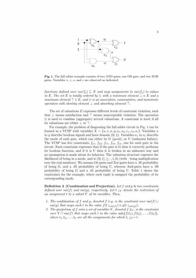
Fig. 1. The full adder example consists of two AND gates, one OR gate, and two XORgates. Variables x, z, s, and c are observed as indicated

functions defined over var(fj) ⊆ X and map assignments to var(fj) to valuesin E. The set E is totally ordered by ≤ with a minimum element ⊥ ∈ E and amaximum element > ∈ E, and ⊕ is an associative, commutative, and monotonicoperation with identity element ⊥ and absorbing element >.

The set of valuations E expresses different levels of constraint violation, suchthat ⊥ means satisfaction and > means unacceptable violation. The operation⊕ is used to combine (aggregate) several valuations. A constraint is hard, if allits valuations are either ⊥ or >.

For example, the problem of diagnosing the full adder circuit in Fig. 1 can beframed as a VCSP with variables X = {u, v, w, y, a1, a2, e1, e2, o1}. Variables uto y describe boolean signals and have domain {0, 1}. Variables a1 to o1 describethe mode of each gate, which can either be G (good), or U (unknown failure).The VCSP has five constraints fa1, fa2, fe1, fe2, fo1, one for each gate in thecircuit. Each constraint expresses that if the gate is G then it correctly performsits boolean function, and if it is U then it is broken in an unknown way andno assumption is made about its behavior. The valuation structure captures thelikelihood of being in a mode, and is ([0, 1],≥, ·, 1, 0) (with · being multiplicationover the real numbers). We assume Or-gates and Xor-gates have a .95 probabilityof being G, and a .05 probability of being U, whereas And-gates have a .99probability of being G and a .01 probability of being U. Table 1 shows theconstraints for the example, where each tuple is assigned the probability of itscorresponding mode.

Definition 2 (Combination and Projection). Let f and g be two constraintsdefined over var(f) and var(g), respectively. Let t ↓Y denote the restriction ofan assignment t to a subset Y of its variables. Then,

1. The combination of f and g, denoted f ⊕ g, is the constraint over var(f) ∪var(g) that maps each t to the value f(t ↓var(f))⊕ g(t ↓var(g));

2. The projection of f onto a set of variables Y , denoted f ⇓Y , is the constraintover Y ∩ var(f) that maps each t to the value min{f(t1), f(t2), . . . , f(tk)},where t1, t2, . . . , tk are all the assignments for which ti ↓Y = t.

4

Given a VCSP and a subset Z ⊆ X of variables of interest, a solution isan assignment t with value ((

⊕mj=1 fj) ⇓Z)(t). In particular, for Z = ∅, the

solution is the value α∗ of an assignment with minimum constraint violation,that is, α∗ = (

⊕mj=1 fj) ⇓∅. For the full adder circuit example, α∗ is 0.044,

corresponding to a single failure either of the Or-gate or of the first Xor-gate.

3 Tree Decomposition

An important class of algorithms for constraint optimization finds solutions bysearching through the space of possible assignments, guided by a heuristic eval-uation function. In the following, we focus on the approach of automaticallygenerating evaluation functions from solutions to smaller subproblems of theoriginal problem. This idea underlies many of the known most efficient searchalgorithms, such as branch-and-bound with mini-bucket elimination (BBMB)[10], best-first search with mini-bucket elimination (BFMB) [9], Russian Dollsearch (RDS) [16], and backtracking with tree decompositions (BTD) [8, 15].

A problem can be broken down into smaller subproblems (”clusters”) bydecomposing the constraint hypergraph H, which associates a node with eachvariable xi, and a hyperedge with the variables var(fj) of each constraint fj .

Definition 3 (Tree Decomposition [6, 11]). A tree decomposition for a prob-lem (X, D, F ) is a triple (T, χ, λ), where T = (V, E) is a rooted tree, and χ, λare labeling functions that associate with each node (cluster) vi ∈ V two setsχ(vi) ⊆ X and λ(vi) ⊆ F , such that

1. For each fj ∈ F , there exists exactly one vi such that fj ∈ λ(vi). For thisvi, var(fj) ⊆ χ(vi) (covering condition);

2. For each xi ∈ X, the set {vj ∈ V | xi ∈ χ(vj)} of vertices labeled with xi

induces a connected subtree of T (connectedness condition).

In addition, we demand that the constraints appear as close to the root of thetree as possible, that is,

3. If var(fj) ⊆ χ(vi) and var(fj) 6⊆ χ(vk) with vk the parent of vi, then fj ∈λ(vi).

Table 1. Constraints for the example (tuples with value 0 are not shown).

fa1: a1 w y fa2: a2 u v fe1: e1 u y fe2: e2 u fo1: o1 v w

G 0 0 .99 G 0 0 .99 G 1 0 .95 G 0 .95 G 0 0 .95G 1 1 .99 G 1 1 .99 G 0 1 .95 B 0 .05 B 0 0 .05B 0 0 .01 B 0 0 .01 B 0 0 .05 B 1 .05 B 0 1 .05B 0 1 .01 B 0 1 .01 B 0 1 .05 B 1 0 .05B 1 0 .01 B 1 0 .01 B 1 0 .05 B 1 1 .05B 1 1 .01 B 1 1 .01 B 1 1 .05

5

Fig. 2. Hypergraph for the example in Fig. 1.

Fig. 2 shows the hypergraph for the example, and Fig. 3 shows two possibletree decompositions.

The separator of a node, denoted sep(vi), is the set of variables that vi shareswith its parent node vj : sep(vi) = χ(vi) ∩ χ(vj). For convenience, we definesep(vroot) = ∅. Intuitively, sep(vi) is the set of variables that connects the sub-problem rooted at vi with the rest of the problem:

Definition 4 (Subproblem). For a VCSP and a tree decomposition (T, χ, λ),the subproblem rooted at vi is the VCSP that consists of the constraints andvariables in vi and any descendant vk of vi in T , with variables of interest sep(vi).

For a tree node vi, we denote solutions to the subproblem rooted at vi byh(vi). The subproblem rooted at vroot is then identical to the problem of findingα∗ for the original COP.

The benefit of a tree decomposition is that each subproblem needs to besolved only once (possibly involving re-using its solutions); the optimal solu-tions can be obtained from optimal solutions to the subproblems using dynamicprogramming. Thus, the complexity of constraint solving is reduced to beingexponential in the size of the largest cluster only.

4 Generating Search Heuristics from Decompositionsusing Dynamic Programming

Kask and Dechter [9, 10] show how the solutions h(vi) to subproblems can beexploited to guide the search for solutions to the original constraint optimizationproblem with variables of interest X.

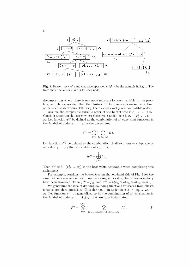
In order to exploit the decomposition during search, the variables must beassigned in an order that is compatible with the tree, namely by first assigningthe variables in a cluster before assigning the variables in the rest of the subprob-lems rooted in the cluster. This is called a compatible order in [8]. For example,for both trees shown in Fig. 1, a compatible order is u, v, w, y, a1, a2, e1, e2, o1.

In [9, 10], the approach to guide search by solutions to subproblems is pre-sented for a so-called bucket trees. A bucket tree is a specialization of a tree

6

Fig. 3. Bucket tree (left) and tree decomposition (right) for the example in Fig. 1. Thetrees show the labels χ and λ for each node.

decomposition where there is one node (cluster) for each variable in the prob-lem, and thus (provided that the clusters of the tree are traversed in a fixedorder, such as depth-first left-first), there exists exactly one compatible order.

Assume the compatible variable order of the bucket tree is x1 ≺ . . . ≺ xn.Consider a point in the search where the current assignment is x1 ← x0

1, . . . , xi ←x0

i . Let function g(i) be defined as the combination of all constraint functions inthe λ-label of nodes v1, . . . , vi in the bucket tree:

g(i) =i⊕

j=1

(⊕

fk∈λ(vj)

fk).

Let function h(i) be defined as the combination of all solutions to subproblemsof nodes c1, . . . , cl that are children of v1, . . . , vi:

h(i) =l⊕

j=1

h(cj).

Then g(i) ⊕ h(i)(x01, . . . , x

0i ) is the best value achievable when completing this

assignment.For example, consider the bucket tree on the left-hand side of Fig. 3 for the

case for the case where u to a1 have been assigned a value, that is, nodes v1 to v5

have been traversed. Then g(5) = fa1, and h(5) = h(v6)⊗ h(v7)⊗ h(v8)⊗ h(v9).We generalize the idea of deriving bounding functions for search from bucket

trees to tree decompositions. Consider again an assignment x1 ← x01, . . . , xi ←

x0i . Let function g(i) be generalized to be the combination of all constraints in

the λ-label of nodes v1, . . . , Vp(xi) that are fully instantiated:

g(i) =Vp(xi)⊗

j=1

(⊗

fk∈λ(vj),var(fk)⊆{x1,...,xi}fk). (1)

7

Let function h(i) be defined as the combination of all functions in the λ-label ofVp(xi) that are not fully instantiated, and all solutions to subproblems of nodesc1, . . . , cl that are children of v1, . . . , Vp(xi), projected on x1, . . . , xi:

h(i) = (l⊗

j=1

h(cj)⊗

fk∈λ(Vp(xi)),var(fk) 6⊆{x1,...,xi}fk) ⇓{x1,...,xi} . (2)

For example, consider the tree on the right-hand side of Fig. 3 and the casewhere the variables {u, v, w, y, a1} have been assigned a value. Then g(1) ⊗ h(1)

with g(1) = fa1 and h(1) = fa2 ⇓u,v ⊗h(v2) ⊗ h(v3) is an (exact) boundingfunction for the value that can be achieved when completing this assignment.

Kask and Dechter [9, 10] present two search algorithms BBMB and BFMBthat exploit this idea of mechanically generating search heuristics from a decom-position of the problem (they also present a way to approximate the heuristics;we will return to this issue in Section 8). The algorithms proceed in two separatephases. First, a pre-computation phase computes the functions h(vi) (solutionsto the subproblems), and then in a second phase, search is guided using the pre-computed values. BBMB uses branch-and-bound search, whereas BFMB usesbest-first (A*) search. It is shown in [9] that, given enough memory, the best-first search variant can outperform branch-and-bound by a factor of 5-10.

5 Demand-Driven Heuristics Computation

However, using a separate phase to pre-compute all functions h(vi) can be waste-ful, because typically only a fraction of the heuristic values will be needed to gen-erate a best solution to the problem. The cost of pre-processing can be avoidedby interleaving the dynamic programming and the search phases with each other.In the following, we call this approach demand-driven heuristics computation inorder to distinguish it from pre-computation of heuristics as in [9, 10].

Recently, [8, 15] have proposed an algorithm called BTD (backtracking withtree decompositions) that achieves interleaving of depth-first branch-and-boundsearch with dynamic programming on tree decompositions. BTD assigns vari-ables along a compatible order, beginning with the variables in χ(vroot). Inside acluster vi, it proceeds like classical branch-and-bound, taking into account onlythe constraints λ(vi) of this cluster. Once all variables in the cluster have beenassigned, BTD considers its children (if there are any). Assume vj is a child of vi.BTD first checks if the restriction of the current assignment to the variables insep(vj) has previously been computed as a solution to the subproblem rooted atvj . If so, the value of this solution (called a “good”) is retrieved and combinedwith the value of the current assignment, thus preventing BTD from solvingthe same subproblem again (called a “forward jump” in the search). Otherwise,BTD solves the subproblem rooted at vj for the current assignment to sep(vj)and the current upper bound, and records the solution as a new good. Its valueis combined with the value of the current assignment, and if the result is belowthe upper bound, BTD proceeds with the next child of vi.

8

In fact, the goods that the BTD algorithm computes correspond to a partialconstruction of the solutions to the subproblems h(vi). BTD thus benefits fromthe complexity bounds of dynamic programming on tree decompositions, whileavoiding the problem of performing dynamic programming prior to search andthus allowing a much smaller average-case complexity. It has been shown [8] thatBTD can outperform BBMB by several orders of magnitude.

6 A* Search with Demand-Driven Heuristics

In the following, we extend the idea of demand-driven heuristics computationfrom depth-first branch-and-bound search to the case of A* search. A* search [7]uses a lower bound g for the partial assignment made so far, and an optimisticestimate h of the value that can be achieved when extending the assignment toall variables. At each point in the search, A* expands the assignment with thebest combined value of g and h. Given the same heuristic, A* search is fasterthan branch-and-bound because it can be shown to expand an optimal numberof search nodes to find the best solution [2].

Combining demand-driven heuristics computation with A* search will thusresult in an algorithm with a time complexity that is optimal among all searchalgorithms having access to the same heuristics. In addition, its space complexityis bounded by dynamic programming and, as we have seen for BTD, typicallymuch lower in the average case.

The main step of extending demand-driven heuristics computation to A*search is to limit the expansion of an A* search node to expanding the next bestchild only, instead of expanding all children of the node. This in turn allows tolimit the computation of heuristics to compute a value for the next best childonly, as illustrated in Fig. 4.

Proposition 1. If g0 ≤ g1 for g0, g1 ∈ E, then for h0 ∈ E, g0 ⊕ h0 ≤ g1 ⊕ h0.

Proof. Because ⊕ distributes over min, min(g0⊕h0, g1⊕h0) = h0⊕min(g0, g1).Because g0 ≤ g1, min(g0, g1) = g0. Thus, min(g0 ⊕ h0, g1 ⊕ h0) = g0 ⊕ h0.

Proposition 1 is an instance of preferential independence [1, 17] and impliesthat in A* search, if the value of a successor node is better than or equal to thevalues of all its siblings, then the siblings cannot immediately lead to solutionsthat have a better value. Consequently, it is sufficient to generate this successornode only and to delay the generation of the siblings, rather than generatingall possible successors at once (see Fig. 4). Exploiting preferential independencecan significantly limit the number of nodes created at each expansion step inA* search. Here, we exploit the idea in the following way: if the expansion of asearch node can be limited to expanding the next best child only, then also thecomputation of a heuristics can be limited to computing a heuristic value for thenext best child only.

9

Fig. 4. Instead of expanding all children of a search node at once (left), preferentialindependence can be exploited to limit expansion to the next best child only (right).Consequently, at each expansion step, it is sufficient to compute a heuristic value forthe next best child only.

Dual Problem Reformulation. However, in order to apply this incrementalexpansion scheme, we need to know in advance which child of the search nodehas the next best valuation g ⊕ h. Unfortunately, in a valued CSP it is not easyto establish such an order among the search nodes a priori, because valuationsare defined for partial assignments (per constraint) rather than for assignmentsto individual variables as in the search tree.

One way to solve this problem is to switch to a dual representation of thevalued CSP, which treats constraints as variables, and tuples of constraints astheir possible domain values. In the dual representation, there are only unarysoft constraints, and binary hard constraints corresponding to equality of sharedvariables (see [13]). Thus, in the dual representation, the desired immediaterelationship exists between assigning a variable – corresponding to assigning atuple to a unary constraint – and obtaining a valuation g.

Approximating the Heuristics. However, which child has the best valuemight then still be affected by the value of the heuristics h; if the heuristic valueh is better for some child than for another, then this child might become thenext best child, even if its value g is worse.

The approach that we use to solve this problem is to choose an heuristicfor A* that is the same for all children of a node. Consequently, if we sort thetuples of the constraints (values in the dual representation) according to theirvaluations, then we will know in advance the order of the children just based ontheir g value. In the dual representation, we can find such an heuristic by simplydropping the hard (equality) constraints from consideration in the heuristics;this heuristic is clearly admissible (optimistic), and has the desired propertythat it is equal for all children of a node.

Distributing the Search Tree. We make one last step that consists of avoid-ing to maintain an explicit A* search tree for each tree node (cluster). Thiswill not reduce the size of the search tree, but allows for processing it in a

10

Fig. 5. Computational scheme for the tree decomposition in Fig. 3. The circled frag-ments correspond to the nodes v1, v2 and v3 of the tree.

distributed way. It is accomplished by replicating each level in the search treeas a constraint (the constraint consists of the current assignments at this levelof the search tree). Thus, computation can proceed independently not only foreach subtree, but also within each tree node (though this is not exploited inour current implementation). For instance, consider again node v1 of the treedecomposition in Fig. 3. In order to find a tuple for this node, the constraintsfa1, fa2, h(v2) and h(v3) have to be assigned a tuple. Instead of maintaining asearch tree with four levels (corresponding to the four constraints), we breakit down using an intermediate function f1 that is the result of combining fa1

and fa2, and an intermediate function f2 that is the result of combining f1 andh(v2). The resulting scheme is illustrated in Fig. 5. In Fig. 5, the bold boxes cor-respond to given constraints, whereas the other boxes correspond to constraintsthat need to be computed. The variable order (sequence of functions in the dualrepresentation) is implicitly encoded in this scheme: each constraint operatorin the network operates as a “consumer” of the constraints of its children, and“produces” a constraint for its parent. We assume two functions producer() andconsumer() that return the producing (preceding) and consuming (succeeding)operator of a constraint, respectively. Function producer() returns nil for givenconstraints at the leaves of the scheme, and function consumer() returns nil forthe constraint fvroot at the root of the tree.

6.1 The BFOB Algorithm

The resulting algorithm can then be understood as best-first, incremental vari-ants of the constraint operators. We illustrate the algorithm by first walkingthrough an example. For instance, a best tuple of the function f3 in Fig. 5is computed as follows: Consider the best tuple of the function fe2, which is〈e2 ← G, u ← 0〉 with value .95 (first tuple of fe2 in Table 1). The projectionof this tuple on u, which is 〈u ← 0〉 with value .95, is necessarily a best tuple

11

function BFOB(s, i)if (i ≤ length(s)) then

return s[i]end ifop ← producer(s)if (op 6= nil) then

case opproj: 〈t, v〉 ← nextBestProj(op)comb: 〈t, v〉 ← nextBestComb(op)

end caseif (〈t, v〉 6= nil) then

append(s,〈t, v〉)return 〈t, v〉

end ifend ifreturn nil

Fig. 6. Function BFOB for best-first search with on-demand bound computation.

of h(v3). Similarly, a best tuple of fa1 can be combined with a best tuple offa2, for instance the first tuples of fa1 and fa2 in Table 1. The resulting tuple〈u ← 0, v ← 0, w ← 0, y ← 0, a1 ← G, a2 ← G〉 is necessarily a best tuple of con-straint f1. This tuple needs to be combined with a tuple of h(v2). A best tuple forh(v2) is generated by combining the best tuple of fo1 with a best tuple of fe1 andprojecting the result onto u, v, w, and y, yielding 〈u ← 1, v ← 0, w ← 0, y ← 0〉with value .90. Since this tuple does not combine with the tuple found for f1

so far, generation of a next best tuple is triggered for both h(v2) and f1. Thenext best tuple of h(v2) is 〈u ← 0, v ← 0, w ← 0, y ← 1〉 with value .90. Thistuple also does not combine with any of the tuples for f1 generated so far.The process continues until a third tuple for h(v2) is generated; for example,by combining the third tuple of fe1 in Table 1 with the best tuple of fo1. Theresulting tuple 〈u ← 0, v ← 0, w ← 0, y ← 0〉 for hv2 combines with the firsttuple that has been generated for f1 and the tuple in h(v3) to a best tuple forfv1 , 〈u ← 0, v ← 0, w ← 0, y ← 0, a1 ← G, a2 ← G〉 with value 0.044. Noticethat in order to compute this best tuple, large parts of the constraints fa1, fa2,fe1, fe2, and fo1 never needed to be visited, and it is not necessary to constructthe constraints h(v2) and h(v3) completely.

Fig. 6 shows the pseudocode of BFOB (best-first search with on-demandbound computation). BFOB(s, i) returns the i-th best tuple of a constraint s,or generates it, if necessary, by calling the constraint operator that producesthe constraint. Each constraint is represented as a list of pairs 〈t, v〉, where t isa tuple and v ∈ A. The tuples are listed in decreasing order according to theirvalue v. Function length() returns the length of the list. Function s[i] returns thei-th tuple-value pair of a constraint s, i ≤ length(s). Function append() appends

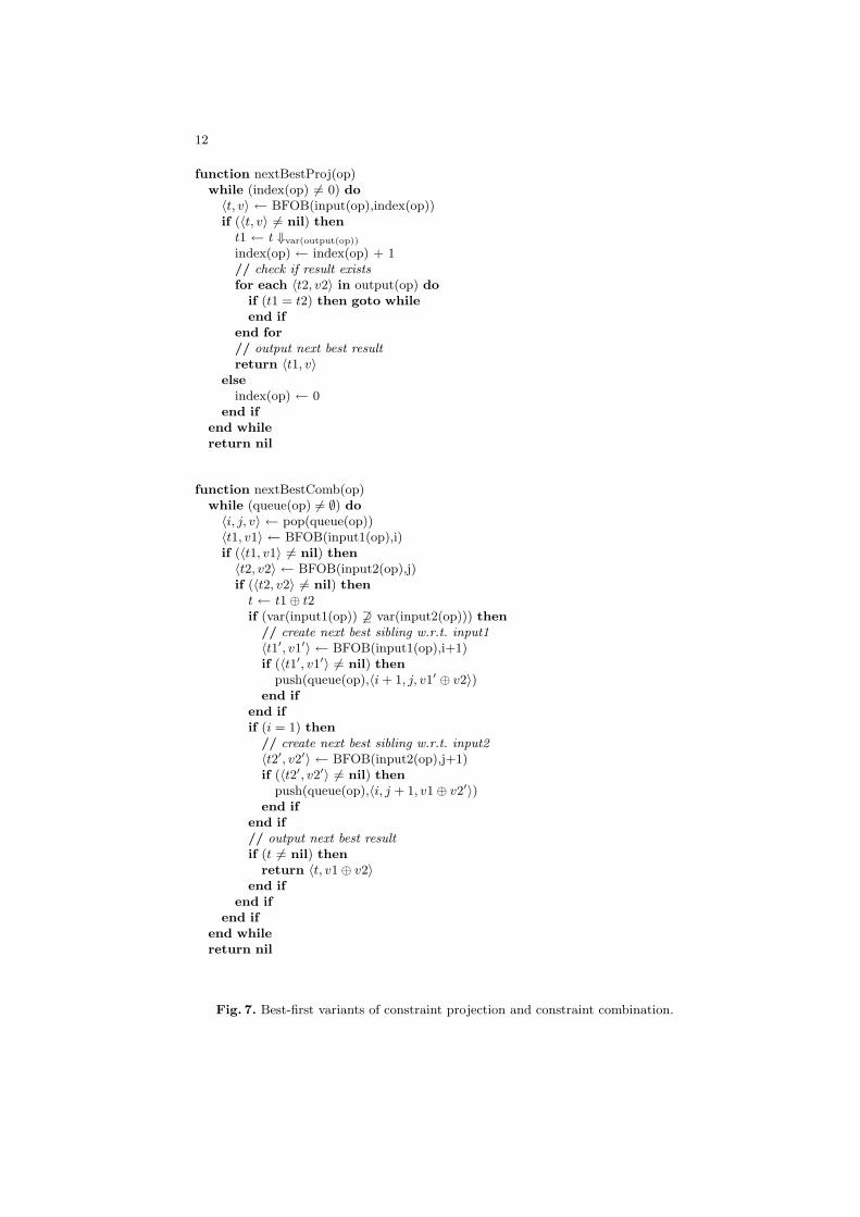
12

function nextBestProj(op)while (index(op) 6= 0) do〈t, v〉 ← BFOB(input(op),index(op))if (〈t, v〉 6= nil) then

t1 ← t ⇓var(output(op))

index(op) ← index(op) + 1// check if result existsfor each 〈t2, v2〉 in output(op) do

if (t1 = t2) then goto whileend if

end for// output next best resultreturn 〈t1, v〉

elseindex(op) ← 0

end ifend whilereturn nil

function nextBestComb(op)while (queue(op) 6= ∅) do〈i, j, v〉 ← pop(queue(op))〈t1, v1〉 ← BFOB(input1(op),i)if (〈t1, v1〉 6= nil) then〈t2, v2〉 ← BFOB(input2(op),j)if (〈t2, v2〉 6= nil) then

t ← t1⊕ t2if (var(input1(op)) 6⊇ var(input2(op))) then

// create next best sibling w.r.t. input1〈t1′, v1′〉 ← BFOB(input1(op),i+1)if (〈t1′, v1′〉 6= nil) then

push(queue(op),〈i + 1, j, v1′ ⊕ v2〉)end if

end ifif (i = 1) then

// create next best sibling w.r.t. input2〈t2′, v2′〉 ← BFOB(input2(op),j+1)if (〈t2′, v2′〉 6= nil) then

push(queue(op),〈i, j + 1, v1⊕ v2′〉)end if

end if// output next best resultif (t 6= nil) then

return 〈t, v1⊕ v2〉end if

end ifend if

end whilereturn nil

Fig. 7. Best-first variants of constraint projection and constraint combination.

13

a tuple t with value v to the constraint. BFOB() is based on the two functionsnextBestProj() and nextBestComb() shown in Fig. 7, that implement best-firstvariants of the constraint operators ⇓ and ⊕, respectively.

Function nextBestProj() in in Fig. 7 consumes an input constraint input().It takes a next best tuple from this constraint, computes its projection, andthen checks whether the resulting tuple already exists on the output constraintoutput(). If the tuple does not already exist, it is a next best tuple of the outputconstraint. An index index() is used to keep track of which tuple from the inputis processed next.

Function nextBestComb() in in Fig. 7 consumes two input constraints in-put1() and input2(). The tuples in the input constraints are combined in abest-first manner using A* search as described above. A search queue queue()is used to keep track of which tuples from input1() and input2() are combinednext. Each entry in queue() is a triple 〈i, j, v〉, where i is the index of a tuple〈t1, v1〉 in input1(), j is the index of a tuple 〈t2, v2〉 in input2(), and v ∈ A is theheuristic value v1⊕ v2 (which is optimistic because it does not take into accountthe hard constraints).

Function nextBestComb() pops an entry with a best value v from the queueand computes the respective combination of tuples from input1() and input2().If the result is not empty (that is, the tuples match), then the combination isa next best tuple of the output constraint. A next best sibling of the entry isgenerated that points to the next entry on stream input1(). For the first tupleof input1(), in addition a next best sibling is generated that points to the nextentry on stream input2(). An optimization is possible for the special case wherethe variables of the constraint of input1() are a superset of the variables ofthe constraint of input2(). In this case (it is known as semi-join), each tuple ofinput2() can combine with at most one tuple of input1(). Hence, no next bestsibling needs to be generated that points to the next tuple of input1().

Initially, the tuples of the constraints are sorted according to their values.For each constraint projection operator, index() is initially set to 1. For eachconstraint combination operator, queue() is initially the singleton {〈1, 1,1〉}.The best tuple of the function fvroot at the root of the scheme, and thus theoptimal solution of the VCSP, can then be obtained by calling BFOB(fvroot ,1).

Theorem 1 (Correctness). The algorithm BFOB is sound, complete, and ter-minates.

Demand-driven heuristics computation is not computationally more complexthan classical dynamic programming methods for best-first search described inSection 3:

Theorem 2 (Complexity). Let (T, χ, λ) be a tree decomposition, T = (V,E).Let w = maxvi∈V (| χ(vi) |)− 1 be the width of the tree decomposition. Then thealgorithm BFOB computes an optimal solution in time O((| F | + | V |)·exp(w))and space O((| V |) · exp(w)).

However, the average complexity of demand-driven function computation canbe much lower if only some best tuples of the resulting function are required.

14

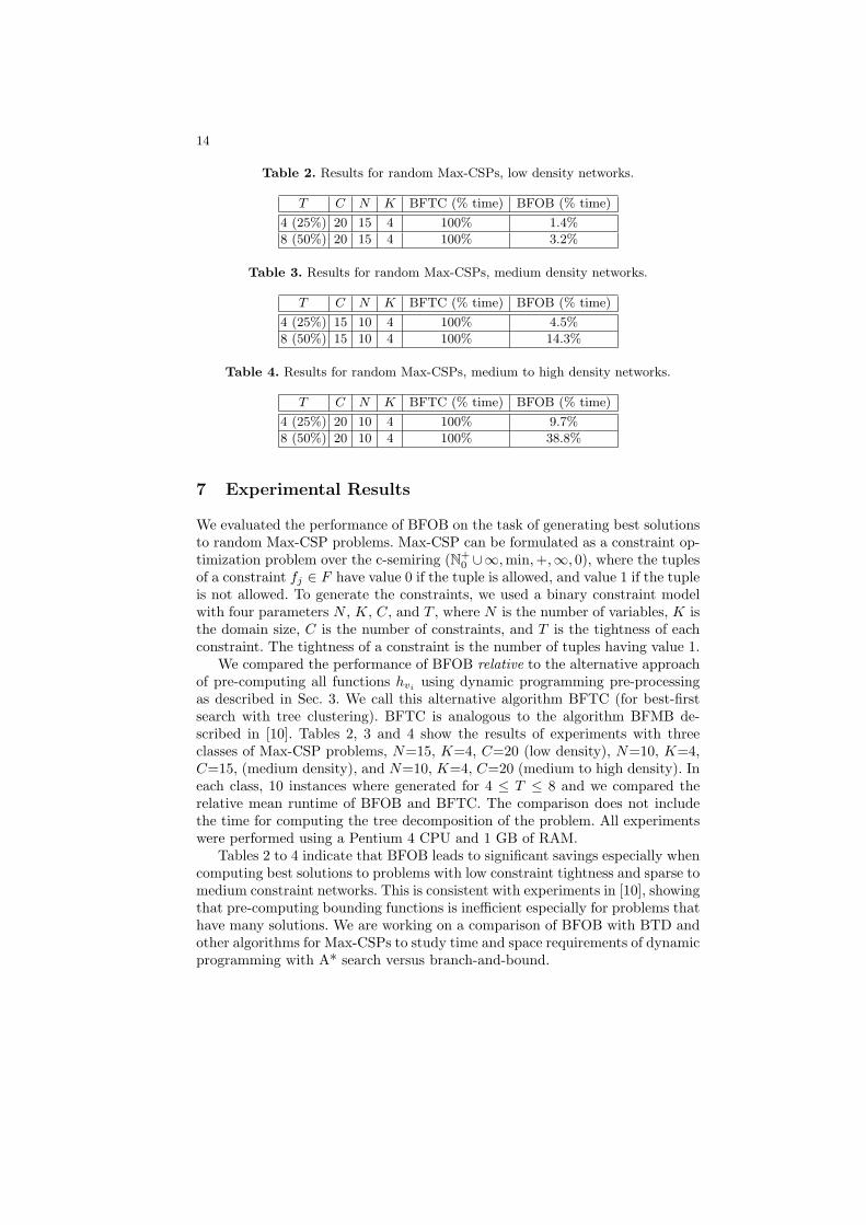
Table 2. Results for random Max-CSPs, low density networks.

T C N K BFTC (% time) BFOB (% time)

4 (25%) 20 15 4 100% 1.4%

8 (50%) 20 15 4 100% 3.2%

Table 3. Results for random Max-CSPs, medium density networks.

T C N K BFTC (% time) BFOB (% time)

4 (25%) 15 10 4 100% 4.5%

8 (50%) 15 10 4 100% 14.3%

Table 4. Results for random Max-CSPs, medium to high density networks.

T C N K BFTC (% time) BFOB (% time)

4 (25%) 20 10 4 100% 9.7%

8 (50%) 20 10 4 100% 38.8%

7 Experimental Results

We evaluated the performance of BFOB on the task of generating best solutionsto random Max-CSP problems. Max-CSP can be formulated as a constraint op-timization problem over the c-semiring (N+

0 ∪∞, min,+,∞, 0), where the tuplesof a constraint fj ∈ F have value 0 if the tuple is allowed, and value 1 if the tupleis not allowed. To generate the constraints, we used a binary constraint modelwith four parameters N , K, C, and T , where N is the number of variables, K isthe domain size, C is the number of constraints, and T is the tightness of eachconstraint. The tightness of a constraint is the number of tuples having value 1.

We compared the performance of BFOB relative to the alternative approachof pre-computing all functions hvi using dynamic programming pre-processingas described in Sec. 3. We call this alternative algorithm BFTC (for best-firstsearch with tree clustering). BFTC is analogous to the algorithm BFMB de-scribed in [10]. Tables 2, 3 and 4 show the results of experiments with threeclasses of Max-CSP problems, N=15, K=4, C=20 (low density), N=10, K=4,C=15, (medium density), and N=10, K=4, C=20 (medium to high density). Ineach class, 10 instances where generated for 4 ≤ T ≤ 8 and we compared therelative mean runtime of BFOB and BFTC. The comparison does not includethe time for computing the tree decomposition of the problem. All experimentswere performed using a Pentium 4 CPU and 1 GB of RAM.

Tables 2 to 4 indicate that BFOB leads to significant savings especially whencomputing best solutions to problems with low constraint tightness and sparse tomedium constraint networks. This is consistent with experiments in [10], showingthat pre-computing bounding functions is inefficient especially for problems thathave many solutions. We are working on a comparison of BFOB with BTD andother algorithms for Max-CSPs to study time and space requirements of dynamicprogramming with A* search versus branch-and-bound.

15

8 Related Work and Discussion

Our algorithm is an adaption of the algorithm BTD by Terrioux and Jegou [15]to the case of A* search. The view in [15] is to improve backtracking by record-ing information (goods) during search; we illustrated how this hybrid approachcan be understood as demand-driven computation of a heuristic using dynamicprogramming. One benefit of this new perspective is that techniques to approx-imate heuristics (bounding functions) become applicable in this framework. Forinstance, Dechter and Rish [4] present a method to decrease the complexity ofbound computation by defining an approximate version of dynamic program-ming called mini-bucket elimination (called mini-clustering in [4] for the moregeneral case of tree decompositions). The idea of mini-bucket elimination is tolimit the size of the computed functions by restricting their maximum arity to afixed value z. This is accomplished by partitioning functions f1, . . . , fk that needto be combined into sets P1, . . . , Pm called mini-clusters, each having a combinednumber of variables less than or equal to z. Then the function (

⊗ki=1 fi) ⇓Y is

bounded by the function f =⊗m

i=1(⊗

fj∈Pi⇓Y ) that applies projection early at

the level of mini-clusters. The accuracy of the approximation can be controlledby varying the parameter z. The algorithm BFMB(z) in [9, 10] combines mini-clustering and best-first search. Lower values for z lead to loose bounds that areeasy to compute, but will guide the search less and therefore necessitate morebacktracking in order to find optimal solutions. Kask and Dechter [10] empir-ically observe an U-shaped performance curve when varying the parameter z,that is, a trade-off between bound accuracy and search. It would be interestingto combine BFOB with approximate bound computation using mini-buckets.This can be accomplished by replacing the scheme of operators and functions(Fig. 5) with an approximate mini-clustering scheme.

A major difference of our approach to the algorithm in [15] is that we usebest-first (A*) search instead of branch-and-bound. A* search is faster thanbranch-and-bound, but it requires more memory. BBMB(z) [10] is a variantof BFMB(z) for branch-and-bound based on bucket trees. BBBT(z) [5] extendsBBMB(z) to tree decompositions. Each time a variable needs to be assigned dur-ing search, BBBT(z) solves the single-variable optimization problem (Z = {xi})for all unassigned variables. That is, like BFOB and BTDval, BBBT(z) inter-leaves dynamic programming and search. Unlike BFOB and BTD, BBBT(z) candynamically change the variable order and prune domains during search. How-ever, BBBT(z) does not compute bounds incrementally on-demand, but insteadstarts a fresh dynamic programming phase at each search node. This can leadto redundant computations, and therefore BBBT(z) and BBMB(z)/BFMB(z)do not dominate each other [5]. Since the algorithm presented in this paperis essentially an improvement of BFMB(z), we expect that BBBT(z) does notdominate BFOB, either. However, variable reordering based on smallest domainsize as in BBBT(z) is not possible in BFOB because the values of variables areonly partially known. An interesting direction for future work would be to ex-tend BFOB such that dynamic programming is not performed on the level ofindividual tuples, but on sets (blocks) of tuples that have the same valuation.

16

9 Summary and Conclusion

Focusing on a few best solutions is an important requirement in many applica-tions. A* search can generate solutions to soft constraints in best-first order, andfaster than branch-and-bound search as it expands a minimal number of searchnodes. However, its memory requirements can make A* search infeasible. Wepresented an algorithm called BFOB that guides A* search for valued CSPs bybounds computed using tree decompositions and dynamic programming. BFOBinterleaves A* search and dynamic programming to compute bounds on-demand,and only to an extent that is necessary in order to generate a next best solu-tion. It thus combines the benefits of A* search with a space complexity that isbounded by structural parameters of the constraint graph, and is even lower inthe average case.

References

[1] Debreu, C.: Topological methods in cardinal utility theory. In: Mathematical Meth-ods in the Social Sciences, Stanford University Press (1959)

[2] Dechter, R., Pearl, J.: Generalized Best-First Search Strategies and the Optimalityof A*. Journal of the ACM 32 (3) (1985) 505–536

[3] Dechter, R., Pearl, J.: Tree clustering for constraint networks. Artificial Intelligence38 (1989) 353–366

[4] Dechter, R., Rish, I.: A scheme for approximating probabilistic inference. Proc.UAI-97 (1997) 132–141

[5] Dechter, R., Kask, K., Larrosa, J.: A General Scheme for Multiple Lower BoundComputation in Constraint Optimization. Proc. CP-01 (2001)

[6] Gottlob, G., Leone, N., Scarcello, F.: A comparison of structural CSP decomposi-tion methods. Artificial Intelligence 124 (2) (2000) 243–282

[7] Hart, P. E., Nilsson, N. J., and Raphael, B.: A formal basis for the heuristic deter-mination of minimum cost paths. IEEE Trans. Sys. Sci. Cybern. SSC-4 (2) (1968)100–107.

[8] Jegou, P., Terrioux, C.: Hybrid backtracking bounded by tree-decomposition ofconstraint networks. Artificial Intelligence 146 (2003) 43–75

[9] Kask, K., and Dechter, R.: Mini-Bucket Heuristics for Improved Search. Proceed-ings of Uncertainty in AI (UAI-99) (1999)

[10] Kask, K., Dechter, R.: A General Scheme for Automatic Generation of SearchHeuristics from Specification Dependencies. Artificial Intelligence 129 (2001) 91–131

[11] Kask, K., et al.: Unifying Tree-Decomposition Schemes for Automated Reasoning.Technical Report, University of California, Irvine (2001)

[12] de Kleer, J.: Focusing on Probable Diagnoses. Proc. AAAI-91 (1991) 842–848

[13] Larrosa, J., Dechter, R.: On the Dual Representation of Non-binary Semiring-based CSPs. Working papers of the Soft Constraints Workshop (SOFT-00), Singapore(2000)

[14] Schiex, T., Fargier, H., Verfaillie, G.: Valued Constraint Satisfaction Problems:hard and easy problems. Proc. IJCAI-95 (1995) 631–637

[15] Terrioux, C., Jegou, P.: Bounded Backtracking for the Valued Constraint Satis-faction Problems. Proc. CP-03 (2003)

17

[16] Verfaillie, G., Lemaitre, M., and Schiex, T.: Russian Doll Search for Solving Con-straint Optimization Problems. In Proc. of the 13th National Conference on ArtificialIntelligence (AAAI-96) (1996) 181–187

[17] Williams, B., Ragno, R.: Conflict-directed A* and its Role in Model-based Em-bedded Systems. Journal of Discrete Applied Mathematics, to appear.