Embed Size (px)
Citation preview

UNIVERSIDAD DE GRANADA
Tesis doctoralNoviembre 2009
A SEARCH FORMECHANISMS PRODUCINGCIRCULAR POLARIZATION
IN COMETS[ PhD THESIS ]
Daniel Guirado RodrıguezInstituto de Astrofısica de Andalucıa (CSIC)
Memoria de Tesispresentada en la Universidad de Granadapara optar al grado de Doctor en Fısica
Directores de tesis:
Dr. Fernando Moreno DanvilaDra. Olga Munoz Gomez

Editor: Editorial de la Universidad de GranadaAutor: Daniel Guirado RodríguezD.L.: GR 2672-2010ISBN: 978-84-693-1999-4


Agradecimientos
Lo difıcil de hacer una lista de agradecimientos es terminarla, por ex-tension y por olvido, ası que aquı va mi lista incompleta. Desen todos losolvidados por agradecidos.
A quienes primero tengo que decir gracias es a Fernando y a Olga, porhaberme ensenado todo lo que hacer falta para ser un cientıfico (otra cosaes que yo haya aprendido algo), por seguir confiando en mı a pesar de midelirio por la procrastinacion, y tambien por su entrega total en este final detesis de Formula 1, en el que ellos lo han pasado peor que yo (lo cierto esque creo que yo he disfrutado, soy adicto a la adrenalina).
A mis companeros del IAA les debo una buena ronda de abrazos dereconocimiento, y a mas de uno un sombrerazo con reverencia, porque hacende este edificio un sitio en el que estoy tan a gusto que hasta tengo uncolchon y unas zapatillas en el despacho. Me divierte pasear por los pasillossalpicando chascarrillos (o escupiendo juramentos, depende del dıa), y tengoen la memoria un buen album de fotos de momentos con cada uno. Jamasse me ocurrirıa destacar a ninguno por encima de los demas. Pero si meobligaran con una pistola a nombrar alguna situacion, me quedo con los ratosde madrugada con Paco Navarro en el pasillo: el enfundado en su pijama, yarreglando el mundo a golpe de cigarro, mientras a mı me faltaba una barradebajo del codo y un vaso en la mano contraria con los que decorar la escena.
El triunvirato es cosa aparte, trasciende lo institucional. Es difıcil que yoconecte con alguien, y mas aun que la conexion sea duradera. Darıo, Charly yEl Boqueron han sido durante cinco anos esos amigos de base que uno hace encada estacion en la que para su tren, y que luego se conservan para siempresin necesidad de un intercambio de favores continuado. Charly gritandosin control, Darıo intentando poner calma, y Miguel Angel “emboqueronao”mientras yo cuento alguna historia, es la la habitual escena de este cuartetode corte marxista (por la rama grouchiana), en el que he tenido la suertede verme involucrado. Gracias por los ratos de chachara en el patio, por lasdoce tapas, por la cana de la una y por las noches de juego impecable. Quesiga este equipo haciendo su magia con el balon, aunque tenga que llevarsecada uno su balon en la maleta.
Tambien he tenido ocasion de viajar en este tiempo de tesis, y conocera gente con duende, de esa que pulsa alguna tecla olvidada del piano dela mente y de pronto te descubre un abanico enorme de nuevas melodıasposibles. Gracias a Joop Hovenier por recibirme y por tratarme siemprecomo a un amigo. No me cabe en la maleta de la memoria todo lo que meha intentado ensenar, pero supongo que ya ire sacando prendas a lo largo delviaje.

Y hablando de viajes, en el viaje de la edad me he encontrado concompaneros que han sido tan decisivos en que yo escriba esta tesis, como eltribunal pertienente que decidiera la concesion de mi beca. Son mis maestrosy profesores desde el colegio. Creo que he tenido una suerte increıblementeinusual, porque guardo un recuerdo excelente de todos. No esta bien destacara nadie, pero yo ya he demostrado sobradamente mi amor por lo inmoral, loilegal, y hasta lo pecaminoso, ası que no me voy a resisir a reconocer que unaparte (la buena) de mi actitud hacia el trabajo y de mi conciencia de equipose la debo a Don Miguel Salvador, a quien le agradezco haberse extralimitadoen sus labores de maestro, y haber ensenado mucho mas que Matematicasy Ciencias Narutales a esa panda de jovenes neandertales submentales sinfuturo entre la que me encontraba yo. Y mi mensaje en la botella es paraJuan Simon. No se a donde gritar esto, Juan, para que lo oigas, pero el 100%de la curiosidad cientıfica que hay en mı me la pegaste tu, y no soy el unico.Ojala te hubiera dicho esto a ti antes, ası podrıa habertelo dicho a ti.
Bueno, tengo una coleccion de amigos que es como un plato de El Bulli :escasa pero exquisita (y una coleccion de enemigos como una enorme fuentede patatas fritas de paquete). Su fidelidad supera mis meritos en el campode la apatıa, y su companıa durante estos anos de tesis me ha devueltoperiodicamente a la estabilidad y a la vida sosegada que requiere este trabajosin horario ni calendario. No caben todos en los dedos de la mano, y sin esatecnica no podre retener la lista completa, ası que solo dire que gracias aMiguel por ser mi hermano, al Consejo de la Fiesta del Vino en pleno pordarme cada ano un dıa imborrable, y a todos los Ana Logica por habermeintegrado en su cuadro de cosas curiosas que contar en los bares, y porhaberme dado una aventura que contar yo cuando ya no tenga edad mas quepara recopilar mis fechorıas.
Pero tambien tengo otro tipo de amigos a los que debo agradecer pro-fundamente un buen porcentaje de lo que queda de mi salud mental tras losanos de elaboracion de esta tesis. Gracias a Groucho Marx, a Woody Allen,a Julio Verne, a Brian Wilson, a Ray Davies, a los 4 Beatles y sus santasmadres, porque aunque ninguno de ellos me conocera jamas, han llenado mitiempo de vida, y no tendre en la vida tiempo de disfrutar de ellos tantocomo sus genialidades se merecen.
Si tengo que hacer una lista de las personas que mas han sufrido estatesis, podrıa dudar sobre la segunda y la tercera, pero la medalla de oro estaclarısima. Gracias, Perez, por devolverme una pluma por cada piedra que tehe lanzado, como los buenos futbolistas. Gracias por tener la solucion antesde que yo tuviera el problema, y sobre todo, gracias por aguantarme y porhacer que parezca facil. Eres la medica que mas sabe de polarizacion circulardel mundo, y yo me hago el chulo hablando de Medicina cuando alguien

comenta su dolencia. “Gracias” no es un premio suficiente a tu labor. Soymal pagador.
El postre se toma al final, porque ası queda el regusto a chocolate, asıque si hiciera falta, este serıa el punto en el que dijera gracias a mis padresy a mis hermanas. Somos cinco marineros en tierra, hipotecados desde hacesiglos por un barco que zozobra mas que avanza, pero que viene cubriendosus rutas puntualmente desde el principio. Aquı tenemos otro puerto en elque parar un rato a tomar un respiro y a beber una jarra de vino antes deseguir con nuestro itinerario inquebrantable. Me alegra haber sido el timonelen esta ocasion.
Y nada mas por hoy (como la cancion de 091 ), no porque no tenga masque decir, sino porque ya es tan tarde que esta amaneciendo (estas cosas hayque escribirlas de noche), y yo ya no podre dormir, como siempre me pasa.


.
A Los Lentejos, que de todos
los que nunca van a leer esta tesis,son quienes mas han puesto en ella.


ResumenEl presente trabajo esta orientado a la busqueda de los mecanismos fısicos quepuedan explicar el grado de polarizacion circular observado en los cometas.Con objeto de establecer una lista de los posibles mecanismos, primero deriva-mos una condicion necesaria para que aparezca un cierto grado de polariza-cion circular no nulo, la cual es que la simetrıa del sistema respecto a ladireccion de la luz incidente debe romperse de alguna manera. El siguientepaso fue identificar los mecanismos que cumplen ese requisito. En primer lu-gar, investigamos el alineamiento de los granos en el coma, que, de hecho, hasido propuesto por varios autores como una posible causa de la polarizacioncircular. Para ello desarrollamos un modelo numerico de alineamiento de losgranos por el viento solar de tipo Monte Carlo. Nuestros resultados mues-tran que las partıculas elongadas se alinean en unas horas, pero el grado depolarizacion circular que se produce es nulo, lo cual es debido a la configu-racion simetrica respecto a la direccion de la luz incidente que se genera porese alineamiento. Como segundo mecanismo, se ha investigado la dispersionsimple de la luz por partıculas asimetricas opticamente inactivas. En estecaso, y para dos partıculas modelo muy concretas, encontramos un nivel delgrado de polarizacion circular resultante del orden de el observado, e inclusomayor. Sin embargo, como quiera que las partıculas en un coma real debenestar distribuidas en una gran cantidad de tamanos y formas, realizamos unaextension de los calculos teniendo en cuenta esta circunstancia. Los resulta-dos fueron negativos, en el sentido de que a medida que en la distribucionse iban anadiendo cada vez mas formas y tamanos, el grado de polarizacioncircular se acercaba cada vez mas a cero. En tercer lugar descartamos la posi-bilidad de que la actividad optica de los materiales que componen el polvodel coma sea la responsable de la polarizacion circular en los cometas. Larazon es que los resultados producidos no encajarıan con algunas de las car-acterısticas encontradas en las observaciones. El cuarto y ultimo mecanismoque propusimos fue el de la dispersion multiple en condiciones de asimetrıarespecto de la direccion de la luz incidente. Para el estudio de este mecan-ismo fue necesario desarrollar un programa de tipo Monte Carlo que simularael transporte radiativo en estas atmosferas. A partir de este programa pudi-mos calcular el flujo y los grados de polarizacion lineal y circular de la luzemergente de un coma cometario, tanto opticamente delgado como grueso, esdecir, en condiciones de dispersion simple o multiple. Despues de estudiar losresultados del codigo para diferentes parametros de entrada que caracterizana la atmosfera cometaria y a la region que se observa, llegamos a la con-clusion de que este mecanismo es el unico que puede producir por sı mismolos niveles observados del grado de polarizacion circular en los cometas.

Abstract
In this work, a systematic study aimed at identifying all possible mecha-nisms producing the observed non-zero degree of circular polarization in thelight scattered by comets is presented. In order to make a list of possiblemechanisms, we first derived a necessary condition, which is that the symme-try of the system around the direction of the incident light must be brokensomehow. Then, we made a search for the mechanisms fulfilling this con-dition. The first mechanism tested was the grain alignment, that has beenproposed by several authors as the cause for the presence of a certain de-gree of circular polarization in comets. To this end, we developed a MonteCarlo model of grain alignment by solar wind particles. We found that elon-gated particles do align in a few hours by this mechanism, but they do notproduce any degree of circular polarization owing to the azimuthally sym-metrical configuration with respect to the direction of the incident light thatresults from the alignment. The second mechanism tested was the singlescattering of light by optically inactive asymmetrical particles. In this case(just for two specific model shapes), we found a significant degree of circularpolarization in the scattered light, comparable to, or even higher than, theobserved. However, in a real cometary atmosphere there must exist a largevariety of asymmetrical particles with different sizes and shapes, so that anextension of these calculations to samples of distributions of asymmetricalparticles of many different sizes and shapes was also conducted. The resultwas negative, in the sense that for the whole sample the degree of circular po-larization tends asymptotically to zero as more and more particles are addedto the system. Third, we ruled out the possibility of the optical activity ofthe materials forming the dust particles of the coma to be responsible forthe degree of circular polarization observed in comets. The reason is thatthe produced results would not match some of the features we found in theobservations. The fourth, and last, mechanism we tried was the presenceof multiple scattering in an azimuthally asymmetrical scenario around thedirection of the incoming light. To accomplish this, a Monte Carlo model ofradiative transfer in cometary comae was developed. The model is capableof giving the flux, and the degree of linear and circular polarization of lightemerging from dusty cometary environments, under conditions of either sin-gle or multiple scattering. After trying several scenarios corresponding todifferent physical parameters of the cometary atmosphere, and different ob-servational conditions, we concluded that the multiple scattering processesare the only mechanism that might give rise to the observed degree of circularpolarization by itself.


Contents
1 Introduction 17
2 Basics on comets 212.1 Definition of comet . . . . . . . . . . . . . . . . . . . . . . . . 212.2 The origin of comets . . . . . . . . . . . . . . . . . . . . . . . 232.3 Composition of the dust . . . . . . . . . . . . . . . . . . . . . 242.4 Size distribution of the particles . . . . . . . . . . . . . . . . . 25
3 Theoretical basis on light scattering 273.1 Some basic definitions . . . . . . . . . . . . . . . . . . . . . . 273.2 Description of light . . . . . . . . . . . . . . . . . . . . . . . . 32
3.2.1 Description of light in terms of the electric field vector 323.2.2 Description of light in terms of the Stokes parameters . 333.2.3 Description of light in terms of flux and degrees of po-
larization . . . . . . . . . . . . . . . . . . . . . . . . . 383.3 Change of the plane of reference . . . . . . . . . . . . . . . . . 413.4 Some general hypotheses . . . . . . . . . . . . . . . . . . . . . 423.5 The light scattering problem . . . . . . . . . . . . . . . . . . . 433.6 The light scattering matrix . . . . . . . . . . . . . . . . . . . . 44
3.6.1 Definition of the light scattering matrix . . . . . . . . . 453.6.2 Some properties of the light scattering matrix . . . . . 483.6.3 Coherency test for the light scattering matrix . . . . . 51
4 Summary of observations 554.1 Introduction . . . . . . . . . . . . . . . . . . . . . . . . . . . . 554.2 Observations of comets . . . . . . . . . . . . . . . . . . . . . . 554.3 Conclusions . . . . . . . . . . . . . . . . . . . . . . . . . . . . 59
5 Candidate mechanisms to produce circular polarization 615.1 Introduction . . . . . . . . . . . . . . . . . . . . . . . . . . . . 615.2 Necessary condition for circular polarization . . . . . . . . . . 62
13

14 CONTENTS
5.3 Possible mechanisms to produce circular polarization . . . . . 63
5.4 Conclusions . . . . . . . . . . . . . . . . . . . . . . . . . . . . 67
6 Circular polarization of light scattered by aligned particles 69
6.1 Introduction . . . . . . . . . . . . . . . . . . . . . . . . . . . . 69
6.2 Mechanism producing the alignment . . . . . . . . . . . . . . 70
6.3 Description of the Monte Carlo bombardment model . . . . . 70
6.4 Results on the alignment . . . . . . . . . . . . . . . . . . . . . 72
6.5 Conclusions . . . . . . . . . . . . . . . . . . . . . . . . . . . . 75
7 Circular polarization of light scattered by asymmetrical modelparticles 77
7.1 Introduction . . . . . . . . . . . . . . . . . . . . . . . . . . . . 77
7.2 How asymmetrical particles produce circular polarization . . . 78
7.3 Description of the model . . . . . . . . . . . . . . . . . . . . . 79
7.4 Choice and description of the numerical method . . . . . . . . 80
7.5 Results and discussion . . . . . . . . . . . . . . . . . . . . . . 83
7.5.1 The effect of changing the size of the particles . . . . . 83
7.5.2 Size distribution . . . . . . . . . . . . . . . . . . . . . . 85
7.5.3 Changing the absorption . . . . . . . . . . . . . . . . . 87
7.5.4 Changing the real part of the refractive index . . . . . 92
7.5.5 Changing the number of monomers of an aggregate ofconstant size . . . . . . . . . . . . . . . . . . . . . . . . 93
7.5.6 Monomers of different sizes in the same aggregate . . . 93
7.5.7 Changing the shape . . . . . . . . . . . . . . . . . . . . 97
7.6 Primary and secondary peaks . . . . . . . . . . . . . . . . . . 100
7.7 Conclusions . . . . . . . . . . . . . . . . . . . . . . . . . . . . 101
8 Circular polarization of light scattered by irregular particles103
8.1 Introduction . . . . . . . . . . . . . . . . . . . . . . . . . . . . 103
8.2 Building the aggregates . . . . . . . . . . . . . . . . . . . . . . 104
8.3 Description and validation of the numerical method . . . . . . 105
8.4 Some examples for individual particles . . . . . . . . . . . . . 106
8.5 Averaging over sizes for individual shapes . . . . . . . . . . . . 108
8.6 Averaging over shapes the size averages . . . . . . . . . . . . . 112
8.7 Conclusions . . . . . . . . . . . . . . . . . . . . . . . . . . . . 112
9 Circular polarization of light scattered by optically activematerials 115

CONTENTS 15
10 Monte Carlo model of radiative transfer in comets 11710.1 Introduction . . . . . . . . . . . . . . . . . . . . . . . . . . . . 11710.2 Multiple scattering as a mechanism to produce circular polar-
ization on a single photon . . . . . . . . . . . . . . . . . . . . 11910.3 Description of the model . . . . . . . . . . . . . . . . . . . . . 120
10.3.1 The particles of the coma . . . . . . . . . . . . . . . . 12010.3.2 Packets of photons . . . . . . . . . . . . . . . . . . . . 12110.3.3 Interaction of a packet of photons with the grains . . . 12410.3.4 Paths of packets of photons . . . . . . . . . . . . . . . 12910.3.5 Light reflection on the nucleus . . . . . . . . . . . . . . 13410.3.6 Common input parameters . . . . . . . . . . . . . . . . 136
10.4 Checking the model . . . . . . . . . . . . . . . . . . . . . . . . 13610.5 The effect of local observations . . . . . . . . . . . . . . . . . 13710.6 Asymmetry of the coma . . . . . . . . . . . . . . . . . . . . . 14210.7 Local observation of an asymmetrical coma . . . . . . . . . . . 14910.8 Conclusions . . . . . . . . . . . . . . . . . . . . . . . . . . . . 152
11 Conclusions 153
12 Future work 157
A General method to sample values of a variable from its prob-ability density function 159


Chapter 1
Introduction
Comets were formed at the beginning of the Solar System formation, andsince their genesis they have remained quite isolated in very clear regions faraway from the Sun and from any other massive body of the Solar System(see Sec. 2.2). Hence, since their beginning, they have been prevented morethan any other type of bodies of the Solar System from heating, from theinteraction with massive planets, and from collisions with other small bodies.Thus, comets are regarded as the most pristine objects in the Solar System,representing the most primitive form of the material out of which all SolarSystem bodies have formed, and giving information on their formation andevolution.
Once they were formed, comets that did not escape from the Solar Systemor crash into any other object, remained moving around the Sun in very farorbits (Sec. 2.2). Eventually, because of some dynamical perturbation, theyare taken out from their orbits and sometimes fall into the inner Solar System,becoming observable from Earth.
The surface features of a comet nucleus cannot be observed from Earthbecause it is just a few kilometers wide (the largest nucleus ever observed wasHale-Bopp’s 40 km across). However, close to the Sun, comets exhibit dustcomae and tails driven by ice sublimation owing to high temperature. Thecoma usually reach dimensions of the order of 104 kilometers and becomeobservable because of light scattered by the dust particles (see Chap. 4).
The study of the composition of the dust contained in comets may giveus some information about the primordial composition of the Solar System.Getting some knowledge about the shape and internal structure of thosegrains may provide us with some clues about the physical processes that thoseparticles underwent during their formation in the primordial Solar System4.6 billion years ago.
A way to carry out such a study is to send a spacecraft to the comet and
17

18 CHAPTER 1. INTRODUCTION
perform in situ measurements or take some samples. Making measurementsand sending the data back to Earth is the goal of the ESA space missionRosetta, which was launched on March 2nd, 2004, and is expected to startorbiting around Comet 67P/Churyumov-Gerasimenko in 2014. The orbiterwill rotate around the coma, but also a lander module will be deployed andwill make measurements on the surface of the nucleus.
Figure 1.1: Rosseta mission module. Credit: ESA.
Another recent space mission to study comets was Stardust, by NASA.It consisted of a probe that travelled to the nearby of Comet P/Wild 2 tocapture some dust grains in an aerogel and send them back to Earth in amodule that landed in the dessert of Utah on January 15th, 2006. Particlescaptured in the aerogel were localized in microscopic pictures with the helpof volunteers, and they were extensively analyzed by NASA scientists (see,e.g., [26]).
Deep Impact was a previous mission performed by NASA. It consisted oncrashing a projectile of 370 kg on the surface of Comet Temple 1 on the 4thof July, 2005. Scientists observed then from Earth the cloud of gas and dustejected from the nucleus
The only remote way of studying a comet is by the light it scatters. Toretrieve information on the physical properties of the scattering particles,we must relate the properties of the observed scattered light to the physicalproperties of the scatterers.
In the present work, we focus on one of the properties of the scatteredlight: circular polarization. Our goal is then to identify the mechanismsgiving the observed degree of circular polarization in comets, i.e., to establish

19
Figure 1.2: Stardust module containing the collected dust particles, just afterlanding in the dessert of Utah, on January 15th, 2006. Credit: NASA.
Figure 1.3: Impact of the Deep Impact projectile on the nucleus of CometTemple 1. Credit: NASA.
which properties of the particles in the coma, or the surface of the nucleus,may explain the observations.
The theoretical basis on comets and light scattering are presented inChaps. 2 and 3 respectively. In Chap. 4 we make a summary of some of theavailable observations of the degree of circular polarization in comets, andpoint out the common properties of all of them and their remarkable features.Once the observations are described and analyzed, we make a theoretical ap-proach to the problem by deriving a necessary condition for a mechanism tocircularly polarize light, and elaborate a list of candidate mechanisms basedon that condition (Chap. 5). Then, the following mechanisms are studied:alignment of non-spherical particles, in Chap. 6, presence of randomly ori-ented asymmetrical grains, in Chaps. 7 and 8, scattering by optically active

20 CHAPTER 1. INTRODUCTION
materials (Chap. 9), and finally, in Chap. 10, multiple scattering by a localnon-central region of a coma. A summary of the general conclusions of thepresent work are presented in Chap. 11, and Chap. 12 contains a list of somework items to be accomplished in the near future.

Chapter 2
Basics on comets
2.1 Definition of comet
Along with asteroids, centaurs, and transneptunian objects, comets belongto the so-called small Solar System bodies category. They can be describedas kilometer-sized irregularly-shaped chunks of dusty ice that develop a shellof sublimated gas with dust, a tail of gas, and another tail of dust when theyapproach the Sun.
A rigorous definition of comets is given by Festou et al. (1993) [19]. Theirdefinition of the different parts of a comet is as follows:
• Nucleus: a kilometer-sized, irregularly shaped, solid body of relativelyloose internal cohesion, consisting of ices (frozen gases; mostly H20)with imbedded dust particles. The nuclei move in elliptical, sometimesnearly parabolic orbits in the solar system. The orbits are basicallyunstable, due to the variable action of the gravitational attraction ofthe planets and are also influenced by ”non-gravitational” forces causedby anisotropic out-gassing from the nuclei.
• Coma: a gaseous and dusty atmosphere around the nucleus which de-velops when it is heated as it approaches the Sun and again abatesduring the outward motion in the orbit. The coma consists of evapo-rated molecules and their daughter products (radicals, atoms, ions) aswell as dust particles released in the same process. Depending on thedistribution of ”active” areas on the surface of the nucleus, comae maybe featureless or highly structured (jets, shells). They shine by atomicand molecular emissions, mostly excited by fluorescence, by sunlightreflected by the dust and by thermal emission at infrared wavelengths.
21

22 CHAPTER 2. BASICS ON COMETS
• Ion tail: consisting of ions which are lost from the coma and acceleratedin the anti-solar direction by action of the interplanetary magnetic fieldcarried by the solar wind. Ion tails shine by the fluorescence from theirions.
• Dust tail: consisting of dust particles lost from the coma and spreadalong the orbit while subjected to pressure of the solar radiation. Dusttails shine by reflected sunlight and thermal infrared emission and theyare an important source of interplanetary material.
Figure 2.1: Comet Hale-Bopp in 1997. The coma is the brightest regionnear the center. Both tails emerge from the coma: the ionic tail (blue),in the anti-solar direction, is due to the interaction of the solar wind withthe gas of the coma, and the dust tail (yellow) is slightly curved owing toradiation pressure. Credit: E. Kolmhofer, H. Raab; Johannes-Kepler-Observatory, Linz, Austria.
The nuclei of comets do absorb almost all light that they receive. Let usdefine the surface albedo of the nucleus as the ratio between the reflected andthe received radiation energy. Some measurements have been performed ofsuch a ratio, and it is of the order of 4% (see, e.g. [32, 33]).

2.2. THE ORIGIN OF COMETS 23
2.2 The origin of comets
Comets are usually divided into two types by the period of their orbit [15]:
1. Short-period comets:
• Less than 200 years period.
• Orbits of 30 - 100 AU in semi-major axis.
• Low inclination of the orbits with respect to the ecliptic plane.
2. Long-period comets
• More than 200 years period.
• Orbits of 10,000 AU or larger in semi-major axis.
• Isotropic distribution of the inclination of orbits.
The generally accepted interpretation of this classification is that there aretwo different origins for comets [15]: Planetesismals forming in the region ofthe Jovian planets were ice-rich, because that zone is beyond the frost line ofthe Solar System. Some of these planetesismals underwent close gravitationalencounters with the Jovian planets, and that made a number of them to becast away in all directions. Some may have completely escaped from the SolarSystem and now are drifting through the interstellar space. The rest endedup in orbits with very large average distances from the Sun. These becameobjects of the Oort cloud, a spherical shell that lies roughly 50,000 AU fromthe Sun. A dynamical perturbation caused, for instance, by a near supernovaexplosion, may take some of these objects out of their orbits and a numberof them could fall into the inner Solar System. This is supposed to be theorigin of the long-period comets. Planetesimals formed beyond Neptune wereeven more ice-rich than those forming among the Jovian planets. They couldnot aggregate into larger bodies because the low density of material in thatzone makes very unlikely an encounter of two objects. As they did not havegravitational interactions with the massive Jovian planets, they remained inthe region where they were formed, building up the so called Kuiper belt.Obviously, the Kuiper belt is quite plane, it coincides with the plane of theecliptic and it starts at the orbit of Neptune (≈ 30 AU). Some of the objectslying in the Kuiper belt may fall into the inner Solar System after any kindof dynamical perturbation of their orbits. This is thought to be the originof the short-period comets. According to this interpretation, short-periodcomets were formed further away than long-period ones.

24 CHAPTER 2. BASICS ON COMETS
Figure 2.2: Sketch of the outer part of the Solar System: the plane regionthat starts at the orbit of Neptune is the Kuiper belt, where short-periodcomets come from. Long-period comets come from the far spherical shell:the Oort cloud. Credit: Stern 2003 [66].
2.3 Composition of the dust
Historically, silicates have been considered the main components of comets,according to infrared spectra. The first detection of the silicate 10−µm bandwas made by Maas et al. in 1970 [41].
In 1997, Kolokolova & Jockers [36] presented a work in which they fittedthe refractive index of the dust particles for the wavelength dependence ofthe linear polarization to coincide with that typically observed in comets.The fit was made based on observations of several comets. They deducedthat cometary dust grains are mainly composed of silicates, with less than1% (in volume) of metallic and carbon inclusions.
A very complete study based on the fit of infrared spectra, and the mea-sured degree of linear polarization of the scattered light at various phaseangles and wavelengths, was carried out by Min et al. in 2005 [48]. Theystudied the composition of Comet Hale-Bopp, and deduced that dust grainswere mainly formed by amorphous carbon (39.1% in volume), amorphousolivine (25.7%) and amorphous pyroxene (18.3%). Crystalline silicicates werealso inferred to be present in comets, but in a much lower abundance. In this

2.4. SIZE DISTRIBUTION OF THE PARTICLES 25
study, silicates are still the primary component, although carbon becomes amain component too.
More recently, much more direct information on the composition of co-metary dust of Comet Wild 2 has been retrieved from Stardust mission. Theanalysis of the sample reveals that silicates are indeed the main components[5, 26], but this time the abundance of carbon is found to be much smallerthat that inferred in [48] for Hale-Bopp.
A very exhaustive work by Kelley & Wooden was recently published [34].They review ground-based and space-based mid-infrared spectra of short-period comets, taken over the last 25 years. They inferred that the silicatecontent of short-period comets might be low relative to other species likeamorphous carbon or FeS. They also claim that short period comets maycontain crystalline silicates, as comets from the Oort cloud (high-temperatureprocesses are needed for the formation of crystals).
In conclusion, silicates appear as the mean component of cometary dustin most works, although amorphous carbon is also considered important insome comets.
Hereafter, we will refer as m to the complex refractive index of anymedium. The imaginary part of m is a measure of the absorption by themedium [7].
2.4 Size distribution of the particles
Suppose a sample made of spherical particles. The number density distribu-tion n(r) at a certain point is defined such as n(r)dr is the fraction of particleswith radii within [r, r + dr] at that point. By definition, it is normalized tounity:
∫ rmax
rmin
n(r)dr = 1. (2.1)
For non-spherical grains, the same definition is valid just by considering theequivalent radius req instead of r (see Sec. 3.1 for definition).
A commonly used model size distribution is the power-law [25]:
n(r) =
c(δ, rmin, rmax)r−δ if rmin ≤ r ≤ rmax,
0 otherwise.(2.2)
The constant c(δ, rmin, rmax) can be obtained from the normalization condi-tion (Eq. 2.1).
In real samples, the size of the grains usually varies through a very widerange of several orders of magnitude. For this reason, it is more convenient
26 CHAPTER 2. BASICS ON COMETS
to make plots using log r for the abscissa, instead of r. However, if weplot n(r) as a function of log(r), we loose the simple interpretation of areasunder the curve as relative number of particles in a certain range of sizes.A commonly adopted solution consists of using a new variable N(log r) suchthat N(log r)dlogr = n(r)dr. The transformation between N(log r) and n(r)is then given by N(log r) = ln 10rn(r).
In situ measurements of the dust size distribution functions are availablefor a few comets only. Thus, measurements by Giotto mission on Halley’sComet dust provided us with a size distribution that could be fitted to apower-law, with exponents varying between -2 and -3.4 approximately [44].Stardust measurements gave a size distribution for Comet Wild 2 that couldalso be fitted to a power-law, resulting in a slightly less steep size distributionthan that for Halley, with particles ranging from 0.01 µm to 1 mm [26].
On the other hand, remote sensing observations of dust tails, and theirinterpretation in terms of models based on dynamical grounds, resulted alsoin time-averaged size distributions that could be fitted to power-law functionswith exponents generally within the range -3 to -3.5 (see, e.g., [31] and [20]).

Chapter 3
Theoretical basis on lightscattering
3.1 Some basic definitions
Hereafter we will use the term light to refer to electromagnetic radiation ofany wavelength, not only visible radiation.
When a solid particle is illuminated by a beam of light, some of theenergy of the incident beam is absorbed (absorption) by the particle (andre-radiated in form of thermal emission), and some of it is scattered in alldirections (scattering). If light is scattered at the same wavelength as theincident light, we will call the scattering elastic scattering. In the limitingcase of scatterers much larger than the wavelength of the incident light, thescattering phenomenon can be divided into three clearly distinguishable pro-cesses: reflection on the surface of the scatterer particle, refraction throughthe particle and diffraction by the borders. Out of this case, these phenomenamix up in such a way that we can just talk about scattering.
In a typical scattering experiment, a cloud of particles is illuminated by abeam of light and an observer sees light scattered in a certain direction (seeFig. 3.1). The plane containing the directions of the incident beam and theobserved scattered light is called the scattering plane. The angle θ formed bythe directions of the observed scattered light and the incident beam is calledthe scattering angle, and the phase angle φ is defined as φ = π − θ. We calloptical axis to the direction of the incident light.
In Fig. 3.2 we show the coordinates system to describe the componentsof the electric field vector of a beam of light. We chose an orthogonal right-handed system (see Eq. 3.1) for vectorial products to be calculated in theusual way [45]. For simplicity, we also imposed that one of the axes lies on
27

28 CHAPTER 3. THEORETICAL BASIS ON LIGHT SCATTERING
Figure 3.1: Sketch of a light scattering event. The scattering plane liesthrough the directions of the incident and observed scattering beams.
the scattering plane, another one is perpendicular to the plane, and the lastone is obviously in the direction of propagation of light. The unit vectorsdefining this system are:
• u in the direction (and sense) of the propagation of light,
• r perpendicular to the scattering plane,
• l through the scattering plane and perpendicular to u and to r in sucha way that
r × l = u (3.1)
The axes choice is not unique, as seen in Fig. 3.2: vectors l′, r′, and ualso fulfill the constrain imposed in Eq. 3.1. Stokes parameters, flux, and thedegree of linear and circular polarization (defined in Secs. 3.2.2 and 3.2.3)are independent of the choice of the system of reference. However, the signsof the components of the electric field vector do depend on that choice.
Let us now define some concepts related to the scatterers:Suppose a particle of arbitrary shape with volume V . Then, the equivalent
radius, req, is defined as the radius of a spherical particle with the samevolume.
req =3
√
3
4πV . (3.2)
Along the present thesis, we will usually refer to req as the size of aparticle.

3.1. SOME BASIC DEFINITIONS 29
Figure 3.2: Orthogonal right-handed reference systems to describe the elec-tric field. Two options are presented: (l,r,u) and (l′,r′,u). Although thesigns of the components of the electric field vector depend on the choice wemake, the observable magnitudes remain the same. The system we assumehereafter is the one plotted with solid lines (l,r,u).
The equivalent size parameter x of a particle is defined as:
x =2πreq
λ, (3.3)
where λ is the wavelength of the incident light (and the scattered light, in caseof elastic scattering). From the electromagnetic point of view, if we equallyscale the size of the scatterers and the wavelength of the incident light with-out changing the shape of the particles, the resulting problem is completelyequivalent to the original one, if the refractive index m of the scatterers isthe same for the new wavelength. This is called the scale invariance rule,and a rigorous proof of it can be found in [50].
Let us introduce now the concept of cross-section. Imagine a large particlebombarded by a plain, uniform and constant stream of small solid projectiles.Let us call F the total energy (kinetic energy of the projectiles) crossing asurface perpendicular to the direction of propagation of the stream per unittime and per unit area. If σ is the projected area of the particle on the planeperpendicular to the incoming stream, then we have:
dE = Fσdt, (3.4)
where dE is the sum of the energy of all projectiles interacting with theparticle in a time interval dt. Now let us change the stream of small solidprojectiles by a beam of light of any wavelength, still plane, uniform andconstant, and let us assume that the particle does not absorb any radiation.By analogy, we define the scattering cross-section σSCA of the particle as:
dE = FσSCAdt. (3.5)

30 CHAPTER 3. THEORETICAL BASIS ON LIGHT SCATTERING
It has dimensions of area. It can be interpreted as follows: the total energyscattered by the particle is equal to the energy of the incident radiation fallingon a surface σSCA perpendicular to the direction of propagation.
We define the geometrical cross-section G of a particle as its projectedarea on a plane perpendicular to the direction of propagation of an incomingbeam of light.
The extensions of these definitions to an ensemble of N particles can bedone simply by adding:
σSCA =N∑
k=1
σkSCA, (3.6)
σkSCA being the scattering cross-section of the k-particle. Obviously, the same
addition relation is valid for the geometrical sections.Contrary to the intuitive interpretation, the scattering cross-section is not
equal to the geometrical cross-section, either for a single particle or for anensemble of particles. Based on this fact, it makes sense the definition of theratio QSCA = σSCA
G: the scattering factor. This magnitude is dimensionless.
Fig. 3.3 shows some examples of the ratio QSCA.As stated before, not only scattering, but also absorption produces the
extinction of light when it interacts with matter. In a way similar to thescattering cross-section, we define the absorption cross-section σABS as thearea such that the total energy absorbed by the particle is equal to theenergy of the incident radiation falling on a surface σABS perpendicular tothe direction of propagation.
The extinction cross-section is just the sum of the scattering and absorp-tion cross-sections. If we directly illuminate a sensor, and then we interposea particle between the light source and the detector, the particle will cast ashadow of area σEXT on the detector. As
σEXT = σSCA + σABS, (3.7)
then:QEXT = QSCA + QABS, (3.8)
where the absorption factor QABS = σABS
Gand the extinction factor QEXT =
σEXT
G.
Both the cross-sections and the factors present a problem: they tell usabout the particles of the cloud of scatterers, but do not contain any infor-mation on how many particles per unit volume are present in that cloud.For that purpose, we define the coefficients as the cross-sections per unitvolume:
KSCA = lim∆V →0
σSCA
∆V, (3.9)

3.1. SOME BASIC DEFINITIONS 31
Figure 3.3: Scattering factor as a function of the size parameter of a singlesphere. The real part of the complex refractive index is Re(m) = 1.33.Results are presented for four values of the imaginary part Im(m). Credit:Hansen & Travis 1974 [25].
KABS = lim∆V →0
σABS
∆V, (3.10)
KEXT = KSCA + KABS = lim∆V →0
σEXT
∆V. (3.11)
The cross sections and the factors are properties of every single particle ofa sample or of the sample as a whole. The coefficients are properties of eachpoint of the space.
The single scattering albedo ω of a particle is defined as:
ω =σSCA
σEXT=
QSCA
QEXT=
KSCA
KEXT. (3.12)

32 CHAPTER 3. THEORETICAL BASIS ON LIGHT SCATTERING
It varies from 0 to 1, and it gives information on how important is thescattering in the extinction. In this way, ω = 1 means that all extinction isdue to scattering and ω = 0 means it is completely due to absorption.
3.2 Description of light
Radiation can be described at three levels. The most complete descriptionconsists of giving the electric (or magnetic) field that constitutes the electro-magnetic wave. For visible radiation this field cannot be directly observed,because its oscillation period is much smaller than the typical duration of ameasurement. Nevertheless, the fields contain all the information about theradiation.
Stokes parameters can be defined as functions of the components of theelectric field (Eqs. 3.34 to 3.37). They consist of four quantities that canbe determined experimentally. By this description, some of the informationcontained in the fields is lost (like the oscillation period of the fields), butall information on the flux and the degree of linear and circular polarization(see Sec. 3.2.3 for definitions) is kept, and the formalism is far more simplethan that based on the fields.
The closest description to the directly observable quantities consists ofan array of three magnitudes: flux, degree of linear polarization and degreeof circular polarization. At this level of description, the information aboutthe dominant direction of vibration of the fields (in case it exists) is lost.
3.2.1 Description of light in terms of the electric field
vector
If we interpose a cloud of particles to a beam of light that propagates in vac-uum, the electromagnetic waves propagating before and after the scatteringevent will be solutions of the Maxwell equations for an homogeneous andisotropic linear medium without any charge distribution, zero-conductivity,and the electric permitivity and magnetic permeability of vacuum. In thiscase, one solution is the monochromatic harmonic plane wave, that fulfillsthe following properties [7]:
1. The wave propagates at speed c = 1√ǫ0µ0
, where ǫ0 and µ0 are the electric
permitivity and the magnetic permeability of vacuum, respectively.
2. Both the electric field vector E and the magnetic field vector B are per-pendicular to the direction of propagation of the wave u in all positionsat all times.

3.2. DESCRIPTION OF LIGHT 33
3. Vectors E and B are perpendicular to each other in all points at alltimes.
4. The amplitudes of the electric and magnetic fields, E0 and B0, arerelated by B0 = 1
cE0.
5. Vectors E and B are in phase in all points at all times.
Statements 2 to 5 can be summarized by the equation:
B =1
cu × E. (3.13)
This means that, in the case of scattering by a cloud of particles in vac-uum, the magnetic field is univocally determined by the electric field. Hence,the incident beam is completely described by:
E = ae−i(kz−ωt+ǫ)E, (3.14)
with E a real unit vector in the direction (and sense) of E, and ǫ the initialphase. We can also write the electric field as a function of its components inthe reference frame defined in Fig. 3.2:
E(r, t) = Ell + Er r,
El = ale−i(kz−ωt+ǫl),
Er = are−i(kz−ωt+ǫr). (3.15)
3.2.2 Description of light in terms of the Stokes pa-rameters
In 1852 George Gabriel Stokes introduced the parameters named after him.The goal of these quantities was to offer a handy way of describing light.
The Stokes parameters for monochromatic light can be defined as func-tions of the components of the electric field vector:
I = ElE∗l + ErE
∗r , (3.16)
Q = ElE∗l − ErE
∗r , (3.17)
U = ElE∗r + ErE
∗l , (3.18)
V = i (ElE∗r − ErE
∗l ) . (3.19)

34 CHAPTER 3. THEORETICAL BASIS ON LIGHT SCATTERING
We call (I, Q, U, V )t the Stokes vector, where t means transpose.Substituting the components of the electric field (Eq. 3.15) in Eqs. 3.16
to 3.19, we can alternatively write the Stokes parameters as:
I = a2l + a2
r , (3.20)
Q = a2l − a2
r , (3.21)
U = 2alar cos (ǫl − ǫr), (3.22)
V = 2alar sin (ǫl − ǫr). (3.23)
In Fig. 3.4, the polarization ellipse is shown. Axes l and r are defined inthe direction and sense of l and r respectively. Light travels into the paper,and the ellipse represents the trajectory of the tip of the electric field vectorthrough time at a fixed position. Inclination is given by angle χ, whichis measured by bringing the positive part of axis l to the mayor semi-axisof the ellipse anticlockwise. Hence, 0 ≤ χ < π. The angle β contains theinformation on the eccentricity of the ellipse and the sense of the polarization.It remains within the interval −π/4 ≤ β < π/4. The modulus of tanβ canbe obtained as the ratio between the minor and the major axes of the ellipse.The sign of β is determined depending on the sense of rotation of the electricfield vector. Along the present study, we do not need to establish a criterionto set the correspondence between the sense of rotation of E and the sign ofβ.
The Stokes parameters can also be written as functions of the quantitiesthat define the polarization ellipse [28] (see Fig. 3.4) as follows:
I = a2, (3.24)
Q = a2 cos 2β cos 2χ, (3.25)
U = a2 cos 2β sin 2χ, (3.26)
V = a2 sin 2β, (3.27)
where a2 = a2l + a2
r . Suppose that the polarization ellipse is oriented withits axes in the directions of the reference axes l and r (see Fig. 3.5). Then,a can be understood as the hypotenuse of the right triangle formed by thesemi-axes of the ellipse. When rotating the reference axes by an angle irot
anticlockwise to (l′, r′), the change of the electric field vector components islike this:
El′ = El cos irot + Er sin irot (3.28)
Er′ = −El sin irot + Er cos irot. (3.29)

3.2. DESCRIPTION OF LIGHT 35
Figure 3.4: Polarization ellipse of a beam of light that propagates into thepaper. The ellipse represents the trajectory of the tip of the electric fieldvector through time at a fixed position. The reference plane is that formedby the axis l and the direction of propagation of light. The inclination of thesemi-major axis of the ellipse with regard to the reference plane is χ, whileβ determines the eccentricity.
Therefore, the amplitudes of the new electric field vector components are:
al′ = al cos irot + ar sin irot (3.30)
ar′ = −al sin irot + ar cos irot. (3.31)
Then, a′2 = a2. We have deduced that a do not depend on the orientationof the reference plane of the polarization ellipse, and as a consequence, it isalways the hypotenuse of the right triangle formed by the semi-axes of theellipse (see Fig. 3.4). Hence, according to Eq. 3.24, I is independent of thescattering plane too, and it is a measure of the size of the polarization ellipse.
Eqs. 3.24 to 3.27 give us a geometrical interpretation of the Stokes pa-rameters: I is a measure of the size of the polarization ellipse. The sign ofV is telling us whether the electric field vector is rotating to the right or tothe left. The magnitude of V informs us about the elongation of the ellipse.V = 0 corresponds to the maximum elongation, when the ellipse becomesa line. While increasing the modulus of V the elongation disappears untilthe ellipse becomes a circle for |V | = I. On the other hand, U vanishes forχ = 0, π/2, and achieves its extreme values for χ = ±π/4, while the oppositehappens to Q. Extreme (either positive or negative) values of Q (or equiva-lently values of U close to zero) are typical of polarization ellipses with theirmajor axis close to the direction of the scattering plane or to its normal.

36 CHAPTER 3. THEORETICAL BASIS ON LIGHT SCATTERING
When values of Q are close to zero, the major axis of the ellipse is close toany of the middle positions between l and r. When U tends to zero, the axesof the ellipse are close to coincide with the axes of the reference system l andr.
An obvious property of the Stokes parameters from their definition (Eqs.3.16 to 3.19) is:
I =√
Q2 + U2 + V 2. (3.32)
In this work we are interested in non-monochromatic light, since thespectra of stars are approximately a black body continuum. For a non-monochromatic beam of light (composed of plane waves of several frequen-cies), the electric field can be written as a plane wave with amplitude andinitial phase variable in time (see Eq. 3.33) [4]. In this case, the Stokesparameters, as defined in Eqs. 3.16 to 3.19, are variable in time. To avoidthis, we now define the Stokes parameters for non-monochromatic light asfollows. If the components of the electric field vector are given by:
El (t) = al (t) e−i(kz−ωt+ǫl(t)),
Er (t) = ar (t) e−i(kz−ωt+ǫr(t)), (3.33)
Figure 3.5: Polarization ellipse (light travelling into the paper) oriented withits axes in the directions of the reference axes l and r. In such an orientation,the hypotenuse of a right triangle formed by the semi-axes of the ellipse isequal to a, where a2 = I, with I written in the axes (l, r). Another systemof axes (l′, r′) is plotted rotated an angle irot anticlockwise with respect to(l, r).

3.2. DESCRIPTION OF LIGHT 37
the Stokes parameters are calculated as the time average of those defined inEqs. 3.16 to 3.19:
I (t) = 〈El (t) E∗l (t) + Er (t) E∗
r (t)〉, (3.34)
Q (t) = 〈El (t) E∗l (t) − Er (t)E∗
r (t)〉, (3.35)
U (t) = 〈El (t) E∗r (t) + Er (t) E∗
l (t)〉, (3.36)
V (t) = i〈(El (t) E∗r (t) − Er (t) E∗
l (t))〉, (3.37)
or, equivalently:
I = 〈al (t)2 + ar (t)2〉, (3.38)
Q = 〈al (t)2 − ar (t)2〉, (3.39)
U = 2〈al (t) ar (t) cos (ǫl (t) − ǫr (t))〉, (3.40)
V = 2〈al (t) ar (t) sin (ǫl (t) − ǫr (t))〉, (3.41)
or:
I = 〈a2 (t)〉, (3.42)
Q = 〈a2 (t) cos 2β (t) cos 2χ (t)〉, (3.43)
U = 〈a2 (t) cos 2β (t) sin 2χ (t)〉, (3.44)
V = 〈a2 (t) sin 2β (t)〉. (3.45)
In all cases the symbols 〈〉 mean average over a time much larger than 2π/ω.The definition for the monochromatic light is a particular case of the onefor non-monochromatic situation, so we can take the latter as the generaldefinition.
Light with constant al/ar and (ǫl (t) − ǫr (t)) is called totally polarizedlight. For this kind of light, the elongation, the inclination and the sense ofthe polarization ellipse remain constant, but its size may change. For totallypolarized light Eqs. 3.42 to 3.45 transform into:
I = 〈a2 (t)〉, (3.46)
Q = 〈a2 (t)〉 cos 2β cos 2χ, (3.47)
U = 〈a2 (t)〉 cos 2β sin 2χ, (3.48)
V = 〈a2 (t)〉 sin 2β. (3.49)
As seen in Eqs. 3.46 to 3.49, Stokes parameters do not remain constant ingeneral for totally polarized light, but the ratio of any pair of them does. Re-garding the polarization ellipse, for totally polarized light it remains constantin shape and orientation, but its size may vary. If the amplitudes and the

38 CHAPTER 3. THEORETICAL BASIS ON LIGHT SCATTERING
initial phases remain constant, the size of the ellipse will remain constant too(monochromatic light). When no correlation exists neither between the am-plitudes nor the initial phases of the components of the electric field, light iscalled totally unpolarized light or natural light : (I, Q, U, V )t = (1, 0, 0, 0)t. Inthis case, the polarization ellipse is not defined in eccentricity, nor in inclina-tion, nor in sense, nor in size. Ratios between any pair of Stokes parametersare not defined either. Between both of these extreme cases (totally polarizedand totally unpolarized light), we find partially polarized light, for which astable average polarization ellipse exists. In this case, ratios between pairsof Stokes parameters vary in time, but they are distributed around a stableaverage.
For the general case of non-monochromatic light the property given inEq. 3.32 is not always valid. A valid property for the general case is (see[28]):
I ≥√
Q2 + U2 + V 2. (3.50)
Another general property, and even more important, is the additivityof the Stokes parameters [28]: If several incoherent light beams (with nocorrelated phases) income on the same point at once, the observed Stokesparameters at that point will be the summation of the Stokes parameters ofall beams.
3.2.3 Description of light in terms of flux and degreesof polarization
Suppose a point source of light emitting radiation in all directions. Twomagnitudes are usually defined to measure how bright the source is:
• Flux : Imagine that we place a detector of elemental area dSdet in a pointP at a certain distance R of the source, with its surface perpendicularto the direction of light. Suppose that an elemental amount of energydE comes onto the detector in an elemental time interval dt. Then, theflux Φ at P is defined by:
dE = ΦdSdetdt. (3.51)
• Intensity : Let us now adopt the same assumptions as in the definitionof the flux, and consider as well that the solid angle subtended by thedetector is dΩdet. Then, the intensity In is defined by:
dE = IndSdetdΩdetdt. (3.52)

3.2. DESCRIPTION OF LIGHT 39
Intensity and flux have the same dimensions. A difference between themis that the intensity does remain constant along the path of light in a mediumwithout absorption, or scattering, or emission (vacuum, for instance). Thereason is that when moving far away from the source along the directionof light, the energy that the detector receives per unit time and per unitarea decreases at the same rate as the solid angle subtended by the source.Let us call W0 the energy emitted by the light source per unit time in alldirections. Then, the energy propagating per unit surface and per unit timeat a distance R from the source is W0
4πR2 . Since the solid angle subtended
by the detector can be written as dΩdet = dSdet
R2 , the intensity is given byIn = W0
4πdS2
detdt
. All factors of the right side of the equation are constant, so
the intensity is constant.In contrast, the flux measured at different distances from the source may
be different. Let us assume a certain solid angle dΩ with its origin in thesource. As light travels in straight lines, the energy of the light propagatinginto the cone defined by dΩ cannot cross the wall to get out of it, and theenergy from the outside cannot enter. Let us assume now that the mediumof propagation does not absorb, or scatter, or emit radiation. Then, theenergy crossing an elemental surface dS per unit time will be the same atall distances, but if R2 > R1, dS2 will be larger than dS1 (dS = R2dΩ).Hence, the energy travelling per unit surface and per unit time decreaseswhile moving far from the source. On the other hand the surface of thedetector dSdet is constant, so according to Eq. 3.51 the flux decreases whilemoving far from the source along the direction of light. Fig. 3.6 illustratesthe difference between flux and intensity.
Along the present work, not intensity, but flux will be used to describelight.
As defined in Eq. 3.34, the first Stokes parameter I is proportional to theflux Φ for a plane harmonic monochromatic wave.
The degree of polarization of a beam of light is defined as:
DP =
√
Q2 + U2 + V 2
I. (3.53)
For totally polarized light DP = 1 (Eq. 3.32) and it is smaller than 1 forany other case (Eq. 3.50).
We define the degree of linear polarization of a beam of light as:
DLP =
√
Q2 + U2
I. (3.54)

40 CHAPTER 3. THEORETICAL BASIS ON LIGHT SCATTERING
Figure 3.6: Light propagating from a point source through a medium withoutabsorption, or scattering, or emission. A detector with a fixed area dSdet islocated at two different distances from the source. Flux is represented onthe left panel. As the energy propagating through a spherical shell per unitsurface and per unit time is smaller for larger distances to the source, and thesurface of the detector remains constant, the flux decreases while increasingthe distance (Eq. 3.51). On the right panel the intensity is represented (seeEq. 3.52 for definition). It is constant along the path of light because whileincreasing the distance to the source, the energy propagating per unit areaand per unit time decreases at the same rate as the solid angle subtended bythe detector.
We refer as the extended degree of linear polarization to:
EDLP =−Q
I=
Ir − Il
Ir + Il, (3.55)
with Il = (I + Q) /2 = E2l and Ir = (I − Q) /2 = E2
r . In case that U = 0,this magnitude in absolute value coincides with the DLP , but it containssome more information: it is positive when the longest axis of the polarizationellipse is close to the perpendicular to the scattering plane, and negative whenit is close to be parallel.
The degree of circular polarization is defined as:
DCP =V
I. (3.56)
For totally polarized light, we deduce from Eqs. 3.46 and 3.49 that the signof the DCP is equal to the sign of β. It is zero when the ellipse becomes aline, i.e., when DLP = 1. The DLP will vanish when the ellipse becomes acircle, i.e., DCP = 1.
We refer as circular polarization (CP hereafter), to the property of lightwith a non-zero DCP . The DCP is the magnitude that accounts for the CP .

3.3. CHANGE OF THE PLANE OF REFERENCE 41
We say that light is left-handed or right-handed circularly polarized when itpossesses a positive or negative DCP respectively (or vice versa, dependingon the criterion). There is no need in this work for establishing a criterion ofcorrespondence between (left-handed,right-handed) circular polarization and(positive,negative) DCP .
3.3 Change of the plane of reference
Let us consider totally polarized light along the present section.In Secs. 3.2.1 to 3.2.3, the scattering plane is assumed as the plane of
reference. Changing the scattering plane would lead to a change in the com-ponents of the electric field El and Er, and equivalently, a change of theparameters defining the polarization ellipse (Fig. 3.4). As a consequence,the Stokes parameters may change, because they are defined as functions ofthe components of the electric field vector (Eqs. 3.34 to 3.37) and also asfunctions of the parameters defining the polarization ellipse (Eqs. 3.42 to3.45). Fig. 3.7 shows a polarization ellipse (light travelling into the paper),along with two systems of reference corresponding to the parallel and per-pendicular axes of two scattering planes. Rotating the axes by an angle irot
anticlockwise produces a change in the orientation of the ellipse, but the sizeand the shape remain the same. As I depends on the size of the polarizationellipse only, and V depends on the size and the shape (see Sec. 3.2.2), thesetwo Stokes parameters remain constant when rotating the reference planearound the direction of light. Parameters Q and U do change, because theydepend on χ:
Q′ = a2 cos 2β cos 2χ′ = Q cos 2irot + U sin 2irot, (3.57)
U ′ = a2 cos 2β sin 2χ′ = −Q sin 2irot + U cos 2irot. (3.58)
Thus, the transformation can be written as:
I ′
Q′
U ′
V ′
=
1 0 0 00 cos 2irot sin 2irot 00 − sin 2irot cos 2irot 00 0 0 1
IQUV
. (3.59)
Although two Stokes parameters change when rotating the scatteringplane, the flux, the DLP and the DCP remain constant. For the flux andthe DCP it is obvious: they only depend on constant parameters I and V .The DLP remains constant because Q2 +U2 does not depend on χ (see Eqs.3.47 and 3.48).

42 CHAPTER 3. THEORETICAL BASIS ON LIGHT SCATTERING
3.4 Some general hypotheses
To set the scenario of the processes we are going to study, we state thefollowing hypotheses:
Vacuum hypothesis : We are interested in studying the scattering of lightby dust particles in the comae of comets. In these systems the density of thegaseous medium that surrounds the scatterers is supposed to be close to zero[10]. As a consequence, for our calculations we can assume that radiationpropagates through vacuum, interacting with dust particles, but never withatoms or molecules of gas.
Natural incident light hypothesis: Throughout this work, we will considerthe light coming from the source to be natural light, i.e., completely unpo-larized. This hypothesis is based on the fact that solar light is unpolarized(see, e.g., [12]).
Monochromatic plane harmonic wave hypothesis: After Fourier’s theorem(see, e.g. [7]), any incident light can be written as the sum of a number ofmonochromatic harmonic waves. Moreover, because of the linearity of the
Figure 3.7: Polarization ellipse (light travelling into the paper), along withtwo systems of axes. The system (l′, r′) is rotated an angle irot anticlockwisewith respect to (l, r). The orientation of the polarization ellipse changeswhen using a different system of reference, but neither the shape nor thesize. This means that changing the plane of reference affects Q and U , butneither I nor V change.

3.5. THE LIGHT SCATTERING PROBLEM 43
Maxwell equations, the total scattered wave will be the sum of the individualscattered waves corresponding to all components of the incident wave. Byjoining both statements we conclude that we can reduce our study to incidentmonochromatic harmonic waves. Furthermore, as comets (scatterers) useto be at distances of the order of the AU (1AU ≈ 1.5 · 1011 m) from theSun (source) and from the Earth (observer), and we are dealing with visiblelight, waves can be considered plane for both the incident and the scatteredbeams in the comet. In summary, we can simplify our work by assumingmonochromatic plane harmonic waves.
Elastic scattering hypothesis : Hereafter, we will consider that the scat-tering is elastic (see Sec. 3.1 for definition). For a dielectric material, thetangential component of the electric field is continuous in the interface be-tween vacuum and the particle [7], what implies that the wavelength of thelight coming onto the particle is the same as that of the scattered light. Ascometary dust grains are mainly formed by dielectric materials (see Sec. 2.3),assuming elastic scattering is reasonable.
3.5 The light scattering problem
In this section we present a summary of the widely used techniques for solvingthe light scattering problem, i.e., for obtaining the properties of the scatteredlight from the properties of the incident light and those of the scatterers.
When x << 1, we say that particles are in the Rayleigh domain. Inthat regime the DCP produced by the scatterers over the scattered light ina single scattering event tends to zero. A complete study of the scatteringproblem in the Rayleigh domain can be found in [35].
In the general case of any size parameter, there are two approaches to theproblem:
1. To think of a particle as a spatial discontinuity in the refractive indexof the medium and solve the Maxwell equations inside and outside thescatterers.
2. To think of a particle as an ensemble of charges affected by the incidentfield and calculate the radiated field.
Based on the first approach, a number of solutions of the scattering prob-lem have been obtained (just for scatterers of simple shapes):
The analytical solution for isotropic and homogeneous spheres was achievedby Lorenz in 1890 [39], and independently by Love in 1899 [40], Mie in 1908

44 CHAPTER 3. THEORETICAL BASIS ON LIGHT SCATTERING
[47] and Debye in 1909 [11]. A solution for optically active spheres can befound in Bohren, 1974 [1]. In 1955, Wait gave a solution for homogeneousand isotropic infinite cylinders [70], which was extended by Bohren in 1978[2] for the case of optically active cylinders. Finally, Oguchi in 1973 [58] andAsano & Yamamoto in 1975 [59] found a general solution for homogeneousand isotropic spheroids.
Also based on the first approach, two more advanced methods were de-veloped. The first one is the T-matrix technique [51], which is devoted tothe calculation of the scattering matrix of rotationally symmetrical particles,either in a fixed orientation or randomly oriented. There is a maximum sizeparameter of particles for which the code can be compiled. The superposi-tion theorem makes it possible to solve the problem for aggregates of sphereswith the T-matrix method [42]. This is a computationally fast algorithmthat calculates accurate results because it makes the orientation average an-alytically. However, it is not able to perform calculations for asymmetricalcompact particles, and there is an upper limit to the size of the grains itcan deal with. The second advanced technique is the Finite Difference inTime Domain (FDTD) method [67], which numerically solves the Maxwellequations by using a finite differences technique. It can calculate the scat-tering matrix of particles of any shape and size, but it is much slower thanthe T-matrix. Its computational requirements (CPU time and memory) risewhen increasing the size of the particles and the accuracy of the calculations,and in case we need an orientation average, it must be done numerically.
Finally, the Discrete Dipole Approximation (DDA) [16] follows the secondapproach. It makes a summation of the fields of the radiant dipoles takinginto account the interaction between them. It is valid for grains of any shapeand any size, but it is very expensive in terms of computational resources.The CPU time increases so fast when increasing the size parameter of theparticles, that the practical size limitation of this method is comparable tothat of T-matrix. Another drawback of DDA is that the orientation averageis made numerically, what implies a lack of accuracy compared to T-matrix.
3.6 The light scattering matrix
Although we do not have an analytical solution for all shapes of the scatterers,we can deduce a general formalism for the scattering problem.

3.6. THE LIGHT SCATTERING MATRIX 45
3.6.1 Definition of the light scattering matrix
Let us assume that the distance R from a particle to the observer of thescattered light is much larger than the maximum length in the scatterer (farfield zone approximation), and also much larger than the wavelength. Then,there exists the linear relation between the electric field vectors of both theincident and the scattered waves in a single scattering event by a singleparticle [50]:
(
Escal
Escar
)
=e−ikR+iǫ0
ikRS (θ, ϕ)
(
Eincl
Eincr
)
, (3.60)
where (R, θ, ϕ) are the spherical coordinates of the position of the observer,the origin being the scatterer cloud and the incident light beam travelling inthe positive sense of the direction of axis z (see Fig. 3.8).
S is the so called amplitude matrix. It is a 2× 2 matrix that depends onthe direction of the scattered beam, the wavelength of the incident beam, theorientation of the scatterer particle and some intrinsic properties of it (size,shape and complex refractive index).
Figure 3.8: Spherical coordinates system assumed to describe the scatteringevent.
From the relation between the incident and scattered fields (Eq. 3.60),we can deduce the relation between the Stokes parameters of the incident

46 CHAPTER 3. THEORETICAL BASIS ON LIGHT SCATTERING
and scattered beams:
Isca =1
k2R2FpIinc, (3.61)
Fp being a 4 × 4 matrix called scattering matrix, given by:
F p11 =
1
2
(
|S11|2 + |S12|
2 + |S21|2 + |S22|
2) , (3.62)
F p12 =
1
2
(
|S11|2 − |S12|
2 − |S21|2 + |S22|
2) , (3.63)
F p13 = Re (S11S
∗12 + S22S
∗21) , (3.64)
F p14 = Im (S11S
∗12 − S22S
∗21) , (3.65)
F p21 =
1
2
(
|S11|2 + |S12|
2 − |S21|2 − |S22|
2) , (3.66)
F p22 =
1
2
(
|S11|2 − |S12|
2 − |S21|2 + |S22|
2) , (3.67)
F p23 = Re (S11S
∗12 − S22S
∗21) , (3.68)
F p24 = Im (S11S
∗12 + S22S
∗21) , (3.69)
F p31 = Re (S11S
∗21 + S22S
∗12) , (3.70)
F p32 = Re (S11S
∗21 − S22S
∗12) , (3.71)
F p33 = Re (S11S
∗22 + S12S
∗21) , (3.72)
F p34 = Im (S11S
∗22 + S21S
∗12) , (3.73)
F p41 = Im (S21S
∗11 + S22S
∗12) , (3.74)
F p42 = Im (S21S
∗11 − S22S
∗12) , (3.75)
F p43 = Im (S22S
∗11 − S12S
∗21) , (3.76)
F p44 = Re (S22S
∗11 − S12S
∗21) . (3.77)
The element F11 is usually called the phase function.The scattering matrix depends on the same variables as the amplitude
matrix. Obviously, as well as the amplitude matrix, the scattering matrix isdimensionless. We would also like to remark that Eq. 3.61 is valid just for asingle scattering event by a single particle, as it was Eq. 3.60, from which itis derived.
Once we set the scattering plane, we can define it as the yz plane, sothat we can set ϕ = 0 (Fig. 3.8). Then, the elements F p
ij of the scatteringmatrix will depend on θ for that scattering plane, and θ is what we definedas the scattering angle in Fig. 3.1. Based on this, from now on we will writethe elements of the scattering matrix as F p
ij (θ). However, it is importantto remark that in general the scattering matrix will be different for differentscattering planes. One exception for this is the case that the sample of

3.6. THE LIGHT SCATTERING MATRIX 47
scatterers is a cloud of randomly oriented particles. Then, all planes areequivalent, so the scattering matrix depends on the scattering angle, but noton ϕ.
So far, we have just talked about scattering by one single particle, but inreal systems we find clouds of dust where lots of particles of different shapes,sizes, compositions and orientations are mixed up. Thanks to the additivityof the Stokes parameters (see Sec. 3.2.2), the formalism for a cloud of scatter-ers is directly derived from the formalism for a single particle: the scatteringmatrix of an ensemble of particles in conditions of single scattering can bewritten as the sum of the scattering matrices of the single particles (Eq.3.79). Single scattering conditions must be imposed because otherwise Eq.3.61 would not be fulfilled, and that equality is used in the proof presentedin Eq. 3.78 (where marked with ∗):
Isca =
N∑
k=1
Iscak
∗=
N∑
k=1
(
Fp
kIinc)
=
(
N∑
k=1
Fp
k
)
Iinc = FIinc. (3.78)
Subindex k means the k-particle of the ensemble. According to Eq. 3.78 thescattering matrix F of an ensemble of N particles is given by:
F =N∑
k=1
Fp
k. (3.79)
For the particular case of natural incident light, Iinc = (I inc, 0, 0, 0)t, just
by using Eq. 3.78 in Eq. 3.56 we see that the DCP can be obtained as:
DCP (θ) =F41 (θ)
F11 (θ), (3.80)
and the EDLP , from Eq. 3.55, is:
EDLP (θ) = −F21 (θ)
F11 (θ). (3.81)
Usually, when more than one kind of particles (shape, size or composi-tion) is present in a cloud of scatterers and the scattering matrix of everysingle type of particles is known, an averaged scattering matrix is used tocalculate the properties of the scattered light given the Stokes parameters ofthe incident light, in conditions of single scattering. The reason for this isderived from Eq. 3.78: The scattering matrix of the whole sample Ftot is thesum of the scattering matrices of all particles in the sample. By using theaverage, we are actually taking 1
NFtot as the scattering matrix of the sample.

48 CHAPTER 3. THEORETICAL BASIS ON LIGHT SCATTERING
That introduces an error factor 1N
in the calculation of the Stokes parameters(Eq. 3.61), but it makes no difference when calculating the DLP , EDLP orDCP , as defined in Eqs. 3.54 to 3.56. In conditions of multiple scatteringthe scattering matrix of the sample is not simply the sum of the scatteringmatrices of the individual grains, so the averaged scattering matrix is not agood approximation to solve the scattering problem.
3.6.2 Some properties of the light scattering matrix
Let us suppose a scattering experiment with a single scatterer in a certainorientation. We call the reciprocal experiment that in which the source andthe observer have been interchanged, but the particle has remained the same.The reciprocal experiment can also be understood in the opposite sense:instead of interchange the source by the observer, we can reorient the grainin such a way that the experiment is the equivalent to the reciprocal. In sucha case we say that we have substituted the particle by its reciprocal particle.
Reciprocity theorem [50]: Suppose that the conductivity, the electric per-mitivity and the magnetic permeability are symmetrical matrices for boththe material the scatterer is made of and the propagation medium. Then,if the amplitude matrix for a scattering experiment in a certain configura-tion is S, it will be [S]−t for the reciprocal experiment. In other words, whenchanging a experiment by its reciprocal, the amplitude matrix is transformedas:
(
S11 S12
S21 S22
)
−→
(
S11 −S21
−S12 S22
)
. (3.82)
As we assumed that the propagation medium is vacuum (Sec. 3.1), we arealways fulfilling half of the hypothesis of the theorem (the part regardingthe propagation medium). The other half (symmetrical matrices for the con-ductivity, the electrical permitivity and the magnetic permeability of thescatterer) means that optically active materials are excluded from the theo-rem.
A transformation in the amplitude matrix directly leads to a transforma-tion of the scattering matrix through Eqs. 3.62 to 3.77. Let us call REC theapplication transforming the scattering matrix F of an scattering experimentinto the scattering matrix Frec of the reciprocal experiment.
The theorem cannot be extended for scattering samples made of manyparticles. By considering the additivity of the scattering matrices (Eq. 3.79):
Frec =
N∑
k=1
Freck =
N∑
k=1
REC (Fk) 6= REC
(
N∑
k=1
Fk
)
= REC (F) , (3.83)

3.6. THE LIGHT SCATTERING MATRIX 49
because REC is not a linear application in the space of 4 × 4 real matrices.So in general, the fact that the reciprocity theorem is valid for every singleparticle of a sample does not assure that it is valid for the whole cloud.
We say that a sample has reciprocity symmetry if for each particle of thesample we can find one (only one) that is the reciprocal of the first.
Suppose a scattering event by a particle. We call the mirror particle ofthe first one to the specular image of it with respect to the scattering plane.If in a sample we change all particles by their mirror particles, the scatteringmatrix transforms as follows:
F11 F12 F13 F14
F21 F22 F23 F24
F31 F32 F33 F34
F41 F42 F43 F44
−→
F11 F12 −F13 −F14
F21 F22 −F23 −F24
−F31 −F32 F33 F34
−F41 −F42 F43 F44
. (3.84)
The proof is simple: Suppose that initially we have a certain scatteringproblem. When changing all particles by their mirror particles, changing thesign of the coordinate Einc
r of the electric field of the incident beam makesthe problem equivalent to the initial scattering problem. Hence, the solutionmust be the same as that of the initial problem, but changing the sign of thecomponent Esca
r of the scattered light, i.e., for the mirror particle:(
Escal
−Escar
)(
S11 S12
S21 S22
)(
Eincl
−Eincr
)
. (3.85)
This is equivalent to:(
Escal
Escar
)(
S11 −S12
−S21 S22
)(
Eincl
Eincr
)
. (3.86)
So the amplitude matrix is transformed as:(
S11 S12
S21 S22
)
−→
(
S11 −S12
−S21 S22
)
. (3.87)
Considering Eq. 3.87 along with Eqs. 3.62 to 3.77, we obtain that thetransformation of the scattering matrix when changing a particle by its mirrorparticle is exactly that in Eq. 3.84.
We say that there is mirror symmetry in a sample if for each particle wecan find one (only one) that is the mirror particle of the first.
Considering the transformations of the scattering matrix when changingto the reciprocal sample (F → REC [F]) and the mirror sample (Eq. 3.84),and considering the additivity of the scattering matrix (Ec. 3.79) as well, itis simple to proof the following properties of the scattering matrix:

50 CHAPTER 3. THEORETICAL BASIS ON LIGHT SCATTERING
1. If there is one (only one) reciprocal particle for each particle of a sample,the scattering matrix can be written as:
F11 F12 F13 F14
F12 F22 F23 F24
−F13 −F23 F33 F34
F14 F24 −F34 F44
. (3.88)
There are left just 10 independent quantities in this matrix (functionsof the scattering angle).
2. If there is one (only one) mirror particle for each particle of a sample,the scattering matrix can be written as:
F11 F12 0 0F21 F22 0 0
0 0 F33 F34
0 0 F43 F44
. (3.89)
There are left just 8 independent quantities in this matrix. In this case,the DCP given by the single scattering of natural light is zero, becauseF41 = 0 (Eq. 3.80).
3. The combination of both of the previous conditions obviously leads to:
F11 F12 0 0F12 F22 0 0
0 0 F33 F34
0 0 −F34 F44
. (3.90)
There are left only 6 independent quantities in this matrix. A realscattering sample is usually made of lots of irregular particles in ran-dom orientation. The random orientation assures that the reciprocitysimplification (Eq. 3.88) can be done in case that the reorientationof the particles is fast enough for a particle to be oriented in both aninitial position and its reciprocal position during the time of a measure-ment. On the other hand, random orientation assures mirror symmetryif particles are symmetrical and again the reorientation is fast enoughfor a particle to orient in both any position and its mirror positionduring one single measurements. However, in most real cases, samplesare made of irregular particles without any plane of symmetry, andsuch particles cannot become their own mirror images by re-orienting.

3.6. THE LIGHT SCATTERING MATRIX 51
In that case, a large amount of different irregular grains is needed inorder to have a particle similar to the mirror image of each one. Withmany different irregular particles we would also have a particle similarto the reciprocal for each one, so the random orientation would not benecessary if the number of irregular grains were high enough. The com-bination of both the presence of many different irregular particles andthe random orientation makes the double approximation (Eq. 3.90) oc-curs in many practical cases, like measurements of scattering matricesof mineral dust samples in the Amsterdam Light Scattering Laboratory[27] and in the new IAA Light Scattering Apparatus in Granada [55].
4. Finally, the most simple scattering matrix is that corresponding tohomogeneous and isotropic spheres [3]:
F11 F12 0 0F12 F11 0 0
0 0 F33 F34
0 0 −F34 F33
. (3.91)
Only 4 independent elements remain for this case.
In the case of Rayleigh scattering, the structure of the grains is not impor-tant, because it cannot be distinguished. As a consequence, in the Rayleighdomain, the same scattering matrix corresponds to particles of all shapesfor a fixed size. In particular, grains of all shapes have the same scatteringmatrix as a sphere (see Eq. 3.91), for a given size. Fig. 3.9 shows an exampleof the independent non-zero elements of the scattering matrix of a sphericalparticle with x = 0.001, normalized to the phase function (the phase functionnormalized to 1 at 30). The refractive index is set to m = 1.5 + i0.001.
3.6.3 Coherency test for the light scattering matrix
A compendium of necessary conditions that scattering matrices must fulfillwas given by Hovenier & Van der Mee in 1996 [29]. In that paper, theyalso put forward a necessary and sufficient condition for a matrix to be ascattering matrix. This condition is called the Coherency test, and was firstproposed by Cloude in 1986 [8]. It is quite a useful test for checking calculatedor measured scattering matrices. If we make a calculation or a measurementof the scattering matrix F corresponding to a certain sample, and the test ispassed, we will not be able to assure that F is the scattering matrix of thesample, but that it will surely correspond to the scattering matrix of somesample.

52 CHAPTER 3. THEORETICAL BASIS ON LIGHT SCATTERING
The test is quite simple to apply. If F = (Fij) is the matrix we want tocheck, its coherency matrix T = (Tij) is defined as:
T11 =1
2(F11 + F22 + F33 + F44) , (3.92)
T22 =1
2(F11 + F22 − F33 − F44) , (3.93)
T33 =1
2(F11 − F22 + F33 − F44) , (3.94)
T44 =1
2(F11 − F22 − F33 + F44) , (3.95)
T14 =1
2(F14 − iF23 + iF32 + F41) , (3.96)
T23 =1
2(iF14 + F23 + F32 − iF41) , (3.97)
T32 =1
2(−iF14 + F23 + F32 + iF41) , (3.98)
T41 =1
2(F14 + iF23 − F32 + F41) , (3.99)
T12 =1
2(F12 + iF21 − iF34 + iF43) , (3.100)
T21 =1
2(F12 + F21 + iF34 − iF43) , (3.101)
T34 =1
2(iF12 − iF21 + F34 + F43) , (3.102)
T43 =1
2(−iF12 + iF21 + F34 + F43) , (3.103)
T13 =1
2(F13 + F31 + iF24 − iF42) , (3.104)
T31 =1
2(F13 + F31 − iF24 + iF42) , (3.105)
T24 =1
2(−iF13 + iF31 + F24 + F42) , (3.106)
T42 =1
2(iF13 − iF31 + F24 + F42) . (3.107)
This matrix has always four real eigenvalues. The test is passed if noneof them is negative.

3.6. THE LIGHT SCATTERING MATRIX 53
Figure 3.9: Independent non-zero relative elements of the scattering matrixof an ensemble of spheres in the Rayleigh regime: x = 0.001. The refractiveindex is set to m = 1.5 + i0.001.

54 CHAPTER 3. THEORETICAL BASIS ON LIGHT SCATTERING

Chapter 4
Summary of observations
Abstract
A compilation of the published observations of the DCP in comets ispresented. Their common properties are emphasized so as to serve as a guidefor the study of the possible mechanisms producing circularly polarized lightin comets.
4.1 Introduction
In the 80’s, at the time of last Halley’s perihelion passage (1986), observa-tions of the DCP of light scattered by comets were no reliable: they stronglydepended on the used instrument (see, e.g., the differences between observa-tions of Halley by Metz & Haefner [46] and Dollfus & Suchail [14]) and inmany cases the errors were comparable to the mean values (see, e.g., [54]).Hence, observations of Comet Halley are not very informative regarding CP .The better information we can retrieve from them is that a persistent non-zero DCP appears in the light scattered by that comet. By the time ofHale-Bopp apparition in 1997, technology had evolved enough so as to re-duce the width of the error bars by a factor 5-10 (see, e.g., [63]). Since then,observations of the DCP in comets have been more frequent, and they havebecome much more informative, because now the error bars are small enoughfor us to recognize features in the curves of the DCP .
4.2 Observations of comets
A list of some significant observations of the DCP of light scattered in cometsis presented below. The more relevant features are pointed out.
55

56 CHAPTER 4. SUMMARY OF OBSERVATIONS
Halley by Morozhenko et al. [54]The authors observed the head of Comet Halley by using a slit of 2.7′′ ×
81′′, which was set sun-ward with respect to comet’s optocenter (it did notcover the nucleus). During the observations, performed in April 1986, thephase angle changed from 34.8 to 21.1 and finally increased up to 27.8.They obtained both positive and negative values of the DCP . For a wave-length of 514 nm, the minimum was (−0.76 ± 0.27)% and the maximum(0.37 ± 0.20)%. Mainly positive values were obtained for a wavelength of484 nm, (−0.05 ± 0.15)% to (0.70 ± 0.28)%). In both cases the DCP wasvery variable in time, not following a constant tendency.
Halley by Metz & Haefner [46]Metz and Haefner [46] carried out other observations of Comet P/Halley
when the phase angle was near 66.1, with a filter centered at a wavelengthof λ = 560 nm. They used three different diaphragms of 10′′, 15′′ and 20′′,with 10′′ corresponding to a length of roughly 9000 km at Halley’s distance.Several parts of the comet were observed: central core, North, South, Eastand West, although no further details are given in the paper regarding theexact location of these regions. The authors obtained values of the DCPin the range (−0.7 ± 0.0)% to (−2.2 ± 0.1)%, which were highly variable ona short time scale (of the order of minutes only). The values of the DCPobtained for the central core did not presented any special feature comparedto those for other regions. In the paper they claimed that the DCP wasreduced by a factor 3 when the aperture of 10′′ was replaced by that of 21′′.
Halley by Dollfus & Suchail [14]Right and left handed CP of the light scattered by various regions of the
coma of Comet P/Halley was also observed by Dollfus and Suchail [14]. Theyused a wide band filter covering the whole visible spectrum. The observedDCP ranged from (−0.65±0.39)% to (1.18±0.48)%. The observations wereperformed when the phase angle varied from 40.7 to 22.5. The DCP wasvery variable in time for the same region. However, a significant decrease ofthe DCP could be noticed when the aperture diameter changed from 7.3”to a wider diaphragm (16.2′′ and 28.1′′). Not a large difference can be foundbetween the observed DCP for diaphragms of 16.2′′ and 28.1′′, because themean values are so small for those slits, that they are comparable to the errorbars. No special values or tendency was found for observations of regions closeto the nucleus of the comet. Dollfus & Suchail suggested in their paper thatresults of observations by Metz & Haefner [46] may need confirmation.
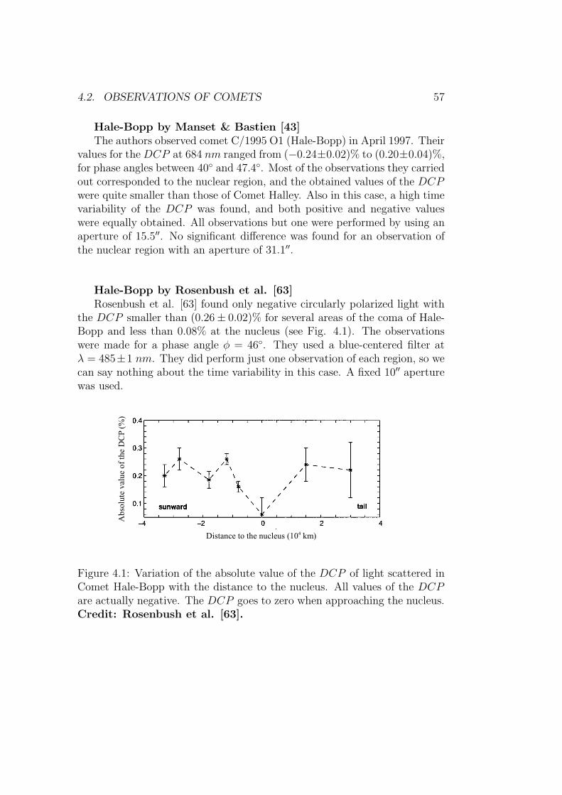
4.2. OBSERVATIONS OF COMETS 57
Hale-Bopp by Manset & Bastien [43]The authors observed comet C/1995 O1 (Hale-Bopp) in April 1997. Their
values for the DCP at 684 nm ranged from (−0.24±0.02)% to (0.20±0.04)%,for phase angles between 40 and 47.4. Most of the observations they carriedout corresponded to the nuclear region, and the obtained values of the DCPwere quite smaller than those of Comet Halley. Also in this case, a high timevariability of the DCP was found, and both positive and negative valueswere equally obtained. All observations but one were performed by using anaperture of 15.5′′. No significant difference was found for an observation ofthe nuclear region with an aperture of 31.1′′.
Hale-Bopp by Rosenbush et al. [63]Rosenbush et al. [63] found only negative circularly polarized light with
the DCP smaller than (0.26± 0.02)% for several areas of the coma of Hale-Bopp and less than 0.08% at the nucleus (see Fig. 4.1). The observationswere made for a phase angle φ = 46. They used a blue-centered filter atλ = 485±1 nm. They did perform just one observation of each region, so wecan say nothing about the time variability in this case. A fixed 10′′ aperturewas used.
Figure 4.1: Variation of the absolute value of the DCP of light scattered inComet Hale-Bopp with the distance to the nucleus. All values of the DCPare actually negative. The DCP goes to zero when approaching the nucleus.Credit: Rosenbush et al. [63].

58 CHAPTER 4. SUMMARY OF OBSERVATIONS
C/1999 S4 (LINEAR) by Rosenbush et al. [62]
The authors observed the DCP of light scattered by this comet in threeseparate observing runs: June 28th - July 2nd, July 8th-9th and July 21st -22nd, 2000, when the phase angle ranged from 60.9 to 122.1. The maximumDCP reached up to ≈ 2%. Both positive and negative values were observedalong the runs: In June 28th, only positive DCP was detected. The nextday, mainly positive values were obtained, and positive and negative wereobserved later, until mainly negative DCP was observed the last two days(see Fig. 4.2). During this evolution, the phase angle was increasing all thetime from 60.9 to 122.1.
Figure 4.2: Empty circles represent the DCP along several cuts through thecoma and nucleus of Comet C/1999 S4 (LINEAR). Filled circles correspondto a fit to the data. Credit: Rosenbush et al. [62].
As shown in Fig. 4.2, for most days, there exists a tendency of the DCP

4.3. CONCLUSIONS 59
to approach zero in the nucleus vicinity.
C/2001 Q4 (NEAT) by Rosenbush et al. [61]
By using a wide R filter and a 10′′ diaphragm (4350 km at the cometdistance), the authors carried out DCP observations of Comet C/2001 Q4(NEAT) from May 21st, 2004 to May 23rd, when the phase angle was φ = 76.The higher observed DCP (in absolute value) was 0.4% approximately. Ahigh variability could be found between the results for the last two days.A general tendency in all days is that the DCP approaches zero near thenucleus region. The curves of the DCP as a function of the distance to thenucleus is shown in Fig. 4.3.
Figure 4.3: DCP along several cuts in coma of Comet C/2001 Q4 (NEAT).Except for the observations corresponding to May 23rd, the DCP approacheszero in the nuclear region. Credit: Rosenbush et al. [61].
4.3 Conclusions
From the observational data reviewed in the previous section, we extract thefollowing conclusions:
• In all cases, the observed DCP for a certain region of the comet ishighly variable in time (day-to-day and even minute-to-minute varia-tions).

60 CHAPTER 4. SUMMARY OF OBSERVATIONS
• The DCP approaches zero when the aperture of the diaphragm in-creases in observations of Halley.
• For accurate observations, such as those of Hale-Bopp, and others ac-quired later, the DCP approaches zero when looking at the nuclearregion of the comet.
• In most cases, both positive and negative values of the DCP are ob-tained, except for two exceptions: observations of Hale-Bopp by Rosen-bush et al. [63], where all obtained values were negative, and observa-tions of Comet C/1999 S4. For the latter case, all observed values werepositive for the smallest phase angle (60.9). Then both positive andnegative values appeared at intermediate values of φ, becoming finallymostly negative at φ ≈ 120.

Chapter 5
Candidate mechanisms toproduce circular polarization
Abstract
Based on symmetry arguments, a necessary condition for an ensemble ofparticles to circularly polarize the scattered light is derived. According tothis condition, a complete list of candidate mechanisms to produce CP isproposed.
5.1 Introduction
Several mechanisms that may give rise to CP in astrophysical environmentshave been historically proposed:
• Alignment of non-spherical particles: this mechanism was first pro-posed by Dolginov & Mitrofanov in 1976 [13]. The possible align-ment mechanisms have been widely studied (see, e.g. [38]), but a goodagreement between the values of DCP observed in comets and calcu-lations for particles aligned by any of these mechanisms has never beenachieved.
• Asymmetrical particles in random orientation: In 2006, Kolokolova etal.[37] found values of the DCP much smaller than the observationsof comets by calculations of single scattering by some irregular aggre-gates composed of identical optically inactive homogeneous spheres inrandom orientation.
• Optical activity : To our knowledge, there are no explicit calculationsof the values that the DCP can achieve if the grains of the coma
61

62 CANDIDATE MECHANISMS
were optically active, although the mechanism is generally invoked asa possible explanation to the observation of the DCP in comets (see,e.g. [62, 61]).
• Multiple scattering : This mechanism is just mentioned by some authorsas a possibility (see, e.g. [46, 62]), but without proof.
We could just have tried the mechanisms listed above and may haveserendipitously found a good agreement between the results on the DCPgiven by any of them and the observations in the scenario we are interested in(comets in our case). However, a rigorous search for the origin of the observedDCP needs for a systematic method to find a complete set of candidatemechanisms, i.e., we must be able to make a list of possible mechanismsgiving rise to CP and assure that the actual responsible of the observedvalues of the DCP is within that list.
To find a complete list we first studied a necessary condition for a mecha-nism to produce CP . Later, we thought about all mechanisms fulfilling thatcondition.
5.2 Necessary condition for circular polariza-
tion1
Let us consider a cloud of particles which is perfectly symmetrical aroundthe direction of the incident light. Such a system possesses certain symme-tries, which means that it remains invariant after certain transformations,for instance the reflection with respect to a plane through the axis of thesystem, and the rotation by π rad about the same axis. Let us assumethat the DCP observed at a certain observation position O1 (Fig. 5.1) isright-handed and consider what happens after applying both of the abovetransformations. By applying the reflection with respect to a plane throughthe system axis we obtain left-handed circularly polarized light when observ-ing from O2, the opposite point of O1 (see left panel of Fig. 5.1). Rotating itby π rad around the axis leads to right-handed CP in O2 (right panel of Fig.5.1). As light cannot be right-handed and left-handed polarized in a certainpoint at the same time, we deduce that the light scattered by a perfectly
1The result given in this section is included in the peer-reviewed publication [24], and itwas presented in three conferences: the 41st annual meeting of the Division for Planetary
Sciences of the American Astronomical Society (oral presentation), the 10th Asteroids,
Comets, Meteors meeting (poster presentation) and the XI Conference on Electromagnetic
& Light Scattering by Non-Spherical Particles (oral presentation).

MECHANISMS 63
azimuthally symmetrical system around the direction of the incident lightcannot be circularly polarized at any scattering direction.
Figure 5.1: Transformations of circularly polarized light observed at a certainpoint, under a mirror symmetry with respect to a plane through the directionof the incident light (left) and upon a rotation by π rad around the samedirection (right). Angles ϕ and θ are the usual spherical coordinates.
The condition deduced above gives us a way to find mechanisms thatmay circularly polarize light: anyone that breaks the symmetry of the systemaround the direction of the incident light is a candidate. As the condition isnecessary, but not sufficient, we cannot be sure that all mechanisms breakingthe azimuthal symmetry are producing CP . We must check them one by one.
5.3 Possible mechanisms to produce circular
polarization
The condition deduced in Sec. 5.2 makes a constrain on the set of candidatesto give rise to the DCP : we just have to look for mechanisms that break thesymmetry around the optical axis. If we enumerate all ways to achieve suchasymmetry we will have a complete list.
The asymmetry of the system around the direction of the incident lightcan be achieved by either the asymmetry of the ensemble of scatteres as awhole (a), the asymmetry of the scatterers individually (b) or both (c). Inour particular case the whole cloud is a comet, and the individual scatterersare the particles of the coma plus the nucleus.
a. Let us assume that the scatterers (both the particles of the coma and thenucleus) are perfectly symmetrical (spherical homogeneous and isotropic

64 CANDIDATE MECHANISMS
grains)2. The only way of such a system to achieve asymmetry is theinhomogeneous distribution of particles in the coma.
We would like to remark the fact that we are calling ”cloud of scatterers”to the part of the comet that the observer is looking at, i.e., if a diaphragmis used to observe a comet, only light coming from a local region will bereceived, so that region will be the cloud of scatterers of the scatteringproblem, instead of the whole comet. This means that even an ensemble ofspherical homogeneous and isotropic scatterers symmetrically distributedaround the direction of light may lead to an asymmetrical scattering sce-nario if the observer focusses only on light coming from a certain part ofthe comet, which is not placed in its center (see Fig. 5.2).
Let us assume that light coming from a non-central local region of a comet(R1 in Fig. 5.2) is circularly polarized by any means. Then, if the comet issymmetrical with respect to the direction of the incident light, the DCPof light coming from the opposite region R2 will cancel that of the lightcoming from R1. Let us prove it: if we observe light coming from R1
and R2 at the same time, we are looking at a system that possesses atleast two symmetries (rotation of π rad around the direction of light andreflection on the plane Π indicated in Fig. 5.2). That is the same scenarioas presented in Sec. 5.2 to prove that an azimuthally symmetrical cometaround the optical axis cannot circularly polarized light. Thus, we deducethat light coming from the system formed by regions R1 plus R2 cannot becircularly polarized when seen from any scattering direction. This meansthat the DCP of light coming from R1 (if it is non-zero by any means),is canceled by that of light coming from R2.
As a corollary, if a region located in the geometric center of the comet isobserved, the DCP of light coming from it must be exactly zero at allscattering directions.
In contrast, according to the previous statements, the local observationof a non-central region of the coma is another candidate mechanism tocircularly polarize light scattered by comets. It is quite important toconsider this mechanism, because polarimetric observations of comets areusually done with a diaphragm so that only photons coming from a smallregion of the comet are taken into account (see Chap. 4).
b. Let us suppose now that the distribution of particles in a comet is perfectly
2In a real situation, however, the particles of the coma may be quite irregular [5], andthe nuclei are known to have irregular shapes, as well as some active areas and jets on itssurface [9].

MECHANISMS 65
Figure 5.2: A non-zero DCP may arise in light coming from any non-centralregion R1 of an azimuthally symmetrical sample. If only that region is ob-served, the possible DCP will not be cancelled by the one of light comingfrom the opposite region R2, so the observer may detect a non-zero DCP .
symmetrical around the optical axis3.
First of all, the grains might be either randomly oriented or not. Here-after we will say that the particles are aligned if the are not in randomorientation, no matter whether they are in a fixed orientation or movingsomehow with less than three rotational degrees of freedom. For instance,we say that a sample of prolate spheroids with their longest axes forming90 with the direction of the incident light and 45 with the x axis arealigned, but the same spheroids randomly oriented in a plane through theoptical axis are aligned too. The alignment of non-spherical particles canbreak the symmetry around the direction of the incident beam, so it isanother mechanism to take into account.
In case that the particles of the coma are randomly oriented they can stillbreak the symmetry of the sample if they are asymmetrical themselves:they have no planes of symmetry (macroscopically and/or microscopi-
3In a real case, the distribution of scatterers is inhomogeneous because of the presenceof active areas and/or jets on the surface of the nucleus [9], for instance.
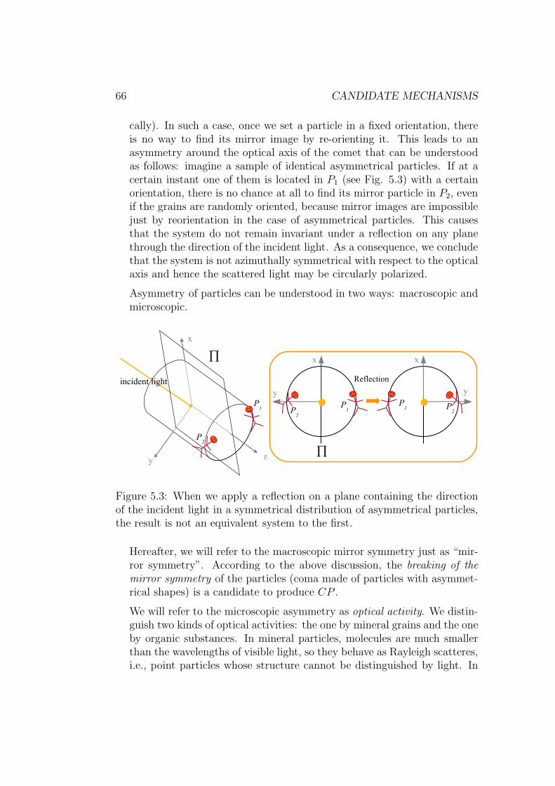
66 CANDIDATE MECHANISMS
cally). In such a case, once we set a particle in a fixed orientation, thereis no way to find its mirror image by re-orienting it. This leads to anasymmetry around the optical axis of the comet that can be understoodas follows: imagine a sample of identical asymmetrical particles. If at acertain instant one of them is located in P1 (see Fig. 5.3) with a certainorientation, there is no chance at all to find its mirror particle in P2, evenif the grains are randomly oriented, because mirror images are impossiblejust by reorientation in the case of asymmetrical particles. This causesthat the system do not remain invariant under a reflection on any planethrough the direction of the incident light. As a consequence, we concludethat the system is not azimuthally symmetrical with respect to the opticalaxis and hence the scattered light may be circularly polarized.
Asymmetry of particles can be understood in two ways: macroscopic andmicroscopic.
Figure 5.3: When we apply a reflection on a plane containing the directionof the incident light in a symmetrical distribution of asymmetrical particles,the result is not an equivalent system to the first.
Hereafter, we will refer to the macroscopic mirror symmetry just as “mir-ror symmetry”. According to the above discussion, the breaking of themirror symmetry of the particles (coma made of particles with asymmet-rical shapes) is a candidate to produce CP .
We will refer to the microscopic asymmetry as optical activity. We distin-guish two kinds of optical activities: the one by mineral grains and the oneby organic substances. In mineral particles, molecules are much smallerthan the wavelengths of visible light, so they behave as Rayleigh scatteres,i.e., point particles whose structure cannot be distinguished by light. In

CONCLUSIONS 67
such a case the asymmetry of the molecules themselves is not important,but the point is the non-symmetrical distribution of them in the particles:grains of crystalline minerals that crystallize in a non-symmetrical systemare microscopically asymmetric. Amorphous minerals or cubic crystals,for instance, are ruled out from the optical activity, because a macro-scopically symmetrical particle made of such materials could become itsown mirror image just by reorientation. Regarding organic materials, thesituation is quite different, because they are made of macromolecules,with sizes quite closer to the wavelengths of visible light than mineralmolecules (so light can distinguish its structure). If these molecules wereasymmetrical (like helixes, for example), they would break the symmetryby themselves as though they were small particles, independently of howthey are distributed into a grain. The optical activity of both mineral andorganic particles is another candidate to give rise CP .
The asymmetry of the nucleus of the comet is also a possibility to breakthe symmetry, around the optical axis. The asymmetry could be due todifferent reasons, such as irregular shape, albedo inhomogeneities, etc.
c. A combination of the above mechanisms would lead to a combination ofasymmetry of the scatterers and the comet as a whole.
We have considered all possibilities, so now we have a complete list ofpossible mechanisms. We will study them in detail in the following chap-ters: alignment of non-spherical grains in Chap. 6, breaking of the mirrorsymmetry in Chaps. 7 and 8, in Chap. 9, optical activity, and finally, localobservation of a non-central region of the comet, inhomogeneous distributionof particles in the coma, and the effect of an asymmetrical nucleus, in Chap.10.
5.4 Conclusions
• The breaking of the symmetry of a comet around the direction of theincident light is a necessary condition for a mechanism to circularlypolarize the scattered light.
• A complete list of candidates to produce CP of light scattered in cometsis the following:
1. Alignment of non-spherical grains.
2. Breaking of the mirror symmetry.

68 CANDIDATE MECHANISMS
3. Optical activity of the material composing the particles.
4. Local observation of a non-central region.
5. Inhomogeneous distribution of particles in the coma.
6. Asymmetrical nucleus of the comet.

Chapter 6
Circular polarization of lightscattered by aligned particles
Abstract
The bombardment of non-spherical grains of the cometary coma by the par-ticles of the solar wind is studied as a mechanism to produce the alignment ofthe grains. It is found that micron-sized elongated particles can be alignedin a few hours by this mechanism. Nevertheless, no CP at all is derivedfrom this alignment because the resulting system is symmetrical around thedirection of the solar incident light.
6.1 Introduction
As we stated in Sec. 5.3, we consider that particles are aligned if they arenot in random orientation, no matter whether they are in a fixed orientationor not.
A long list of possible mechanisms for aligning particles has been proposedsince Dolginov & Motrofanov paper in 1976 [13]. In that paper the authorsalready proposed four possible mechanisms for the alignment of dust in thecoma of comets: paramagnetic relaxation, gas streams and interaction ofthe solar radiation and the solar wind with the grains. They deduced underrestrictive assumptions that the particles in the part of the coma turnedtowards the Sun are aligned by radiative pressure, and the DCP of thescattered light could reach 4% for silicate-like particles. After that paper, aconsiderable progress has been made regarding the alignment mechanisms:a recent complete review can be found in [38]. In spite of this, it is not clearyet if the alignment really happens in cometary comae, and, in case it takesplace, what mechanism is the main responsible for that.
69

70 ALIGNMENT OF PARTICLES
6.2 Mechanism producing the alignment
If the alignment of non-spherical particles is the cause of the observed DCPof light scattered in comets, the mechanism that aligns particles must be fast,because a non-zero DCP is observed in the coma, even in regions relativelyclose to the nucleus, and most of the particles in that zone were ejected fromthe surface of the nucleus just some hours or days before [9]. As resultscoming from previous works are not conclusive (see Sec. 6.1), we decided tomake an investigation by our own. We did not try to study all alignmentmechanisms one by one because this is beyond the scope of the present work.Instead, we wondered how would grains align and what would it be thetypical alignment time for some simple mechanism over some simple kind ofparticles. We considered rectangular prisms as grains of the coma, and wedeveloped a Monte Carlo model of bombardment by particles of the solarwind in order to simulate their alignment. So the alignment mechanism thatwe studied was interaction of dust particles with the solar wind. We chosethis one for two reasons:
• Comets, when observed, are located at a distance from the Sun of theorder of the AU , where the interaction of the dust grains of the comawith the solar wind may be significant.
• To our knowledge, there are not explicit calculations of the alignmenttime of particles by the interaction with the solar wind. Thus we wantedto make a contribution to the solution of the problem of the alignmentby this study.
6.3 Description of the Monte Carlo bombard-
ment model
First of all, as we just wanted to investigate the effect of the alignment ofthe particles, we considered a cometary nucleus and a distribution of grainsin the coma that are azimuthally symmetrical around the direction of light.Let us now carefully describe what kind of dust particles of the coma weassumed, what are the parameters describing the solar wind and how theparticles of the solar wind interact with the dust grains.
• Dust particles : For simplicity we supposed a comet located at 1AUfrom the Sun. The reason for that is that at this position, the solarwind is well characterized and it has a significant effect.

BOMBARDMENT MODEL 71
We chose rectangular prisms (compact particles) as dust grains. Weused two shapes: a prolate prism with axes ratios 1:1:2 (A) and anoblate prism with 2:2:1 (B). We set the dimensions of the particle (A)as 0.1 µm× 0.1 µm× 0.2 µm. The dimensions of (B) are calculated sothat the volumes of both particles (A and B) are equal. We assumed adensity of 3 gcm−3 for the grains. This is a typical value for silicates,and we already stated that silicates are one of the main components ofthe cometary dust (see Sec. 2.3).
As we did not have any information on the initial state of rotationof the grains, we supposed a certain initial angular velocity insteadof assuming the particles to be at rest. In this way, the alignmentmay be slower than for particles at rest, and we wanted to considerthe most unfavorable scenario. We assumed an initial angular velocityω0 = 0.7 rad s−1. The actual initial rotation velocity might be muchhigher, for instance, if the grains are dragged by a stream of gas ejectedat high velocity from the surface of the nucleus. However, we do nothave any quantitative information about this effect. The best we coulddo was to assume an scenario closer to reality than having the particlesat rest at t = 0. We took as the initial rotation axis the longest,because that corresponds to the more stable rotational state, and wesupposed that particles quickly go to that state by dissipating heat.The dissipation could take place because grains are not perfect solidbodies, and there might be some internal frictions when particles aredeformed due to rotation. Particle (A) was initially set with its longestaxis parallel to the direction of incidence of the flux, and particle (B)started the simulation oriented with its shorter axis parallel to the flux.
• Solar wind : We assumed two important hypotheses:
1. The particles of the solar wind propagate in a uniform and con-stant flux in the direction (and sense) of light. Here, we are implic-itly making the assumption that the solar wind is not significantlydeviated from the radial direction of propagation by the magneticfield.
2. The particles of the solar wind interact with the dust grains ofthe coma as if the grains were in vacuum, i.e., it is assumed thatthere is no interaction of the solar wind with the gas. We basedthis hypothesis in the low vapor density of the coma.

72 ALIGNMENT OF PARTICLES
Table 6.1 shows the main characteristics of the solar wind at 1AU [57].
Composition 50% electrons,48% protons, and2% ions He+
Velocity vF 350 kms−1
Flux density 3 · 108 cm−2s−1
Table 6.1: Some properties of the solar wind used in the model of bombard-ment.
• Interaction: Collisions were considered completely inelastic. This hy-pothesis simplifies the calculations, as in this way we know that a solarwind particle transfers all its angular momentum to the dust grain ithits. Hence, the increment of the angular momentum of a grain aftera collision is dL = r × pp, where pp is the linear momentum of theparticle of solar wind before the collision (pp = mvF, where vF is thevelocity of incidence of the solar wind particle and m is its mass). FromdL, the new angular momentum of the grain is given as L′ = L + dL.Then, by calculating the inverse of the inertia tensor I of the grain, weobtain its new angular velocity as ω = I−1L. With the new angularvelocity, we apply a differential rotation, and get the position of thegrain an elemental time dt later. This process is repeated with parti-cles sequentially randomly hitting on the visible side of the grain, atthe rate given by the flux density specified in Table 6.1.
To quantify the alignment of the grains, we define two orthogonal systemsof reference. One is fixed in the particle and the other one is external. Thesystem fixed in the particle has its axes coincident with the principal axes ofthe prism. The external system of reference has the z axis in the directionof propagation of the solar wind, but in the opposite sense (see 6.1).
6.4 Results on the alignment
As shown in Fig. 6.2, the prolate grain (A) is aligned with its longest axisperpendicular to the direction of the incident flux. Despite its initial orien-tation was the most unfavorable to achieve the alignment, it happens in lessthan 1.8 · 104 s. Once it is aligned, (A) quickly rotates around its longestaxis, and that axis slowly randomly rotates around the direction of the so-lar wind. As shown in Fig. 6.3, the oblate prism is not aligned even in a
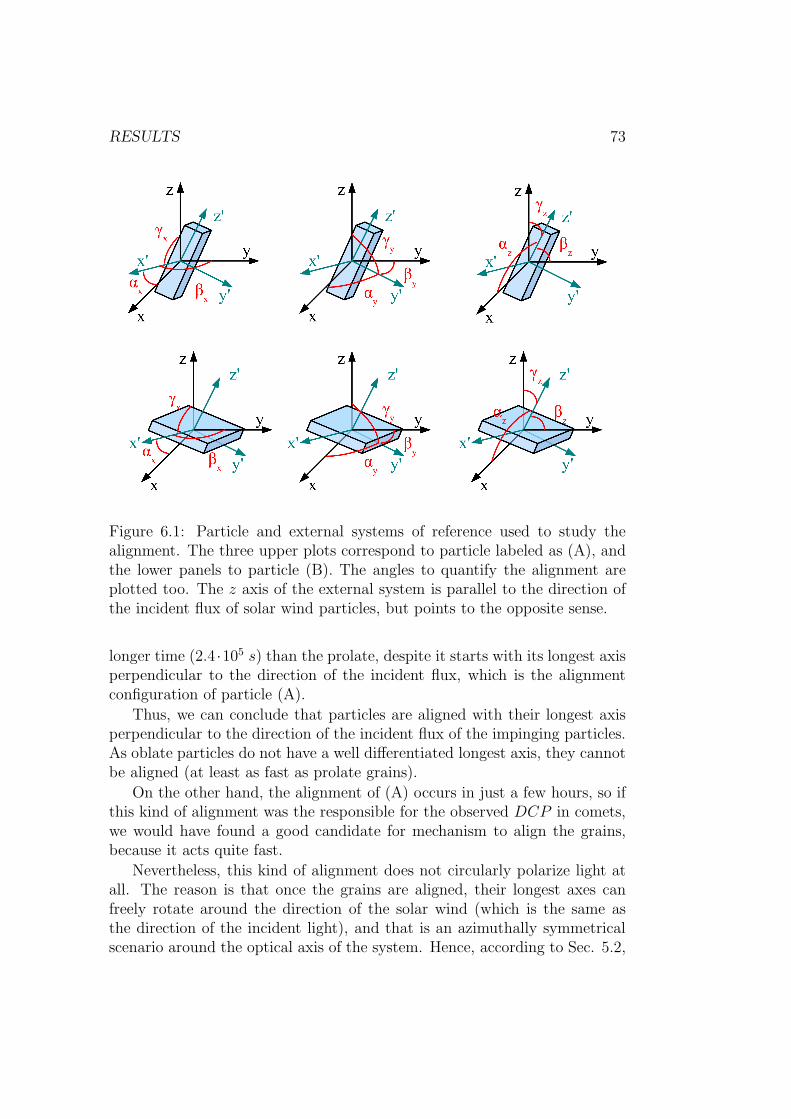
RESULTS 73
Figure 6.1: Particle and external systems of reference used to study thealignment. The three upper plots correspond to particle labeled as (A), andthe lower panels to particle (B). The angles to quantify the alignment areplotted too. The z axis of the external system is parallel to the direction ofthe incident flux of solar wind particles, but points to the opposite sense.
longer time (2.4 ·105 s) than the prolate, despite it starts with its longest axisperpendicular to the direction of the incident flux, which is the alignmentconfiguration of particle (A).
Thus, we can conclude that particles are aligned with their longest axisperpendicular to the direction of the incident flux of the impinging particles.As oblate particles do not have a well differentiated longest axis, they cannotbe aligned (at least as fast as prolate grains).
On the other hand, the alignment of (A) occurs in just a few hours, so ifthis kind of alignment was the responsible for the observed DCP in comets,we would have found a good candidate for mechanism to align the grains,because it acts quite fast.
Nevertheless, this kind of alignment does not circularly polarize light atall. The reason is that once the grains are aligned, their longest axes canfreely rotate around the direction of the solar wind (which is the same asthe direction of the incident light), and that is an azimuthally symmetricalscenario around the optical axis of the system. Hence, according to Sec. 5.2,

74 ALIGNMENT OF PARTICLES
Figure 6.2: Evolution of the rotation of the prolate grain of dimensions0.1 µm × 0.1 µm × 0.2 µm and density of 3 gcm−3, under bombardmentby the solar wind. In less than 1.8 · 104 s, it is aligned with its longest axisperpendicular to the direction of the incident flux.
no CP can be achieved by this mechanism.

CONCLUSIONS 75
Figure 6.3: Evolution of the rotation of the oblate particle with axes ratios2 : 2 : 1, and the same volume and density as (A), under bombardment bythe solar wind. There is no alignment in 2.4 · 105 s.
6.5 Conclusions
• Prolate rectangular prisms of dimensions 0.1 µm×0.1 µm×0.2 µm witha density of 3 gcm−3 are aligned in 1.8 · 104 s due to the bombardment

76 ALIGNMENT OF PARTICLES
by the solar wind particles at an heliocentric distance of 1AU .
• The alignment occurs with the longest axis of the particle orientedperpendicularly to the direction of the incident light.
• Oblate particles with the same volume and density as the prolate ones,but with axes ratios 2:2:1, are not aligned even in 2.4 · 105 s.
• If particles in comets were actually aligned and the responsible mech-anism for the alignment was the bombardment by the solar wind, wewould not obtained any non-zero DCP , because the cloud of alignedparticles would be symmetrical around the direction of the incidentlight.
Chapter 7
Circular polarization of lightscattered by asymmetricalmodel particles
This chapter is based on the peer-reviewed paper by Guirado et al. entitled Circular
polarization of light scattered by asymmetrical particles [22]. Some of theses results were
presented in the IX Conference on Electromagnetic & Light Scattering by Non-Spherical
Particles.
Abstract
To clarify the possible contribution of asymmetry of particles to CP incomets, some calculations of the DCP of light singly scattered by some kindsof asymmetrical model particles were performed. We considered aggregatesof optically inactive homogeneous identical spheres in random orientation.We analyzed the effect of changing the size of the particles, and performeda size average. The effect of changing the refractive index and the shape ofthe grains was studied too. The values of the computed DCP are generallyin the range of the observed ones for light scattered by comets (Chap. 4).
7.1 Introduction
As we stated in Sec. 5.3, if the particles in the coma of a comet are asym-metrical, there is a chance for the scattered light to be circularly polarized,even if the grains are in random orientation and homogeneously distributedaround a symmetrical nucleus.
Along this chapter we will be dealing with the calculation of the maxi-mum DCP that a sample of randomly oriented asymmetrical particles can
77

78 ASYMMETRICAL MODEL PARTICLES
produce. Since we are primarily interested in the application to the cometaryenvironment, we will assume similar sizes and refractive index as have beenfound for dust in comets (see Secs. 2.4 and 2.3). In this chapter, our purposeis not to build a realistic model of a cometary coma to try to reproduce theobservations. Instead, we just want to develop the most simple model thatcan tell us whether or not we must rule out single scattering by opticallyinactive asymmetrical particles in random orientation as a mechanism pro-ducing a significant DCP in comets. If we obtain very small values of theDCP compared to the observations by assuming a very asymmetrical modelparticle, this mechanism can be ruled out. If we obtain values of the DCP ofthe order of the observations or larger, we will give another step by buildingup a more realistic model.
In Sec. 7.2 we explain the theoretical basis of the mechanism that makesasymmetrical particles circularly polarize the scattered light. Sec. 7.3 con-tains the description of the model, and Sec. 7.4 includes an analysis of someavailable codes to perform the required calculations plus a brief review of thecomputational method that we finally chose. Numerical results are shownand discussed in Sec. 7.5. Finally, in Sec. 7.7, the main conclusions aregiven.
7.2 How asymmetrical particles produce cir-
cular polarization
We already discussed in Sec. 5.3 that, based on the condition given in Sec.5.2, the presence of asymmetrical particles in the coma of a comet may leadto a certain DCP of the scattered light. In this section, we present anotherproof of the possibility of having CP by this mechanism. This proof is basedon symmetry arguments applied to the Stokes parameters. It is just validfor the breaking of the mirror symmetry, and we are presenting it in orderto better understand how the mechanism works.
Suppose a collection of randomly oriented asymmetrical particles illumi-nated by a plane-parallel beam of unpolarized light with flux vector (1, 0, 0, 0)t.The flux vector of the singly scattered light at a certain distance, can gen-erally be written as (a, b, c, d)t, using the scattering plane as the plane ofreference for the Stokes parameters. This flux vector depends on the scatter-ing angle and the properties of the scattering particles. In what follows wekeep the scattering angle fixed. Let us now replace each particle by its ownmirror particle, but keeping the incident light unchanged. Because of sym-metry, the scattered beam will become the mirror image with respect to the
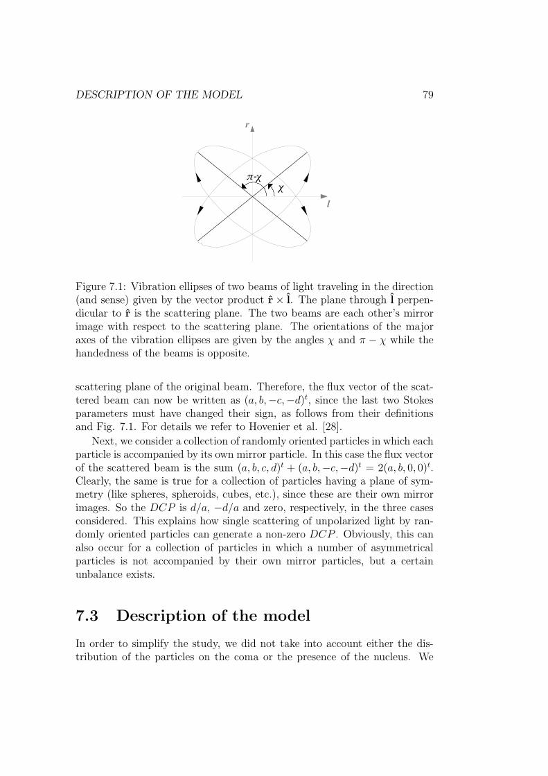
DESCRIPTION OF THE MODEL 79
Figure 7.1: Vibration ellipses of two beams of light traveling in the direction(and sense) given by the vector product r × l. The plane through l perpen-dicular to r is the scattering plane. The two beams are each other’s mirrorimage with respect to the scattering plane. The orientations of the majoraxes of the vibration ellipses are given by the angles χ and π − χ while thehandedness of the beams is opposite.
scattering plane of the original beam. Therefore, the flux vector of the scat-tered beam can now be written as (a, b,−c,−d)t, since the last two Stokesparameters must have changed their sign, as follows from their definitionsand Fig. 7.1. For details we refer to Hovenier et al. [28].
Next, we consider a collection of randomly oriented particles in which eachparticle is accompanied by its own mirror particle. In this case the flux vectorof the scattered beam is the sum (a, b, c, d)t + (a, b,−c,−d)t = 2(a, b, 0, 0)t.Clearly, the same is true for a collection of particles having a plane of sym-metry (like spheres, spheroids, cubes, etc.), since these are their own mirrorimages. So the DCP is d/a, −d/a and zero, respectively, in the three casesconsidered. This explains how single scattering of unpolarized light by ran-domly oriented particles can generate a non-zero DCP . Obviously, this canalso occur for a collection of particles in which a number of asymmetricalparticles is not accompanied by their own mirror particles, but a certainunbalance exists.
7.3 Description of the model
In order to simplify the study, we did not take into account either the dis-tribution of the particles on the coma or the presence of the nucleus. We

80 ASYMMETRICAL MODEL PARTICLES
considered a sample of optically inactive particles in random orientation andcalculated the DCP after single scattering of natural light. So, instead ofbuilding a radiative transfer model of the comet, we just calculated the scat-tering matrix of a sample of randomly oriented particles of a certain size,shape and refractive index, and then apply Eq. 3.80 to obtain the DCP ,(also Eq. 3.81 to obtain the EDLP ).
As we were interested in obtaining the largest possible DCP , we usedsome model particles especially designed with very asymmetrical shapes. Theused particles are described in each section. Although compact grains havebeen proven to explain many of the observed properties of cometary dust [52],we used aggregates of spheres for our calculations because of the followingreason: We needed accurate calculations since the observed values of theDCP are close to zero. Moreover, we needed to calculate the DCP for thelargest possible particles in order to approach the sizes of the real grains incomets (see Sec. 2.4). The T-matrix technique for aggregates of spheres is thebest choice to solve this problem, because it makes the orientation averageanalytically, so it is more accurate and faster than the other methods (seeSec. 3.5).
Hereafter, when we refer to aggregates, we will denote by x the sizeparameter of the monomers of the particle, and by X the size parameterof the whole aggregate.
Along the present chapter, we will consider a wavelength λ = 500 nm.
7.4 Choice and description of the numerical
method
There exist at least two public available codes implementing the T-matrixtechnique for multi-spheres: Mackowki & Mishchenko’s [42] and Xu’s [71].In this section, we present an a analysis to determine which one is the mostappropriate for our calculations of the DCP . For such purpose, we madesome comparisons between T-matrix and DDA, and we eventually comparedresults from both implementations of T-matrix.
The more widely checked DDA code is the one developed by Draine &Flatau [17], although a recent new implementation by Yurkin & Hoekstra[72] has arisen, which introduces some numerical improvements that reducethe CPU time and memory consumption for calculations (see comparisonin [60]). However, this new code has not been optimized yet for randomlyoriented particles, and regarding this type of calculations it gives less accurateresults than Draine’s code [60]. Thus, we chose Draine’s implementation of

NUMERICAL METHOD 81
the DDA method.
Figure 7.2: Asymmetrical model particle used for comparison of DDA andMackowski & Mishchenko’s T-matrix method. It is composed of 7 monomers.All monomers are equal in size and refractive index.
First of all, we compared DDA Draine’s results with those by Mackowski& Mishchenko’s T-matrix code. We used as a test particle the one describedin Fig. 7.2. We chose m = 1.5 + i0.001 as refractive index. Figs. 7.3 and 7.4show the calculated DCP for the particle in random orientation for two sizes:x = 0.5 and x = 1 respectively (or X = 0.96 and X = 1.91). In both caseswe built the particle with 69443 dipoles for DDA calculations. The choice ofthe large number of dipoles was made to fulfill the criterion |m|kd < 0.1 (see[17] for an explanation). For calculations of flux and the EDLP , |m|kd < 0.5is enough, as stated in [17], but for the DCP we need better accuracy. Wemade an average over 16000 orientations.
There is a good agreement between the results given by both methods,so we can rely on both of them to calculate the DCP as a function of thescattering angle with high accuracy.
In any case, we also checked Xu’s code by comparing its results to Mack-owki & Mishchenko’s. We used the particle defined in the right panel ofFig. 7.5. The size parameter of each monomer was set to x = 1, so the sizeparameter of the whole grain became X = 2.92. This time we calculated theEDLP for the particle in random orientation (Fig. 7.6) as well as the DCP(Fig. 7.7) by both Mackowski & Mishchenko’s and Xu’s codes for multi-spheres. We found significant discrepancies when comparing the computedresults to each other, especially in the DCP . This means that one of the

82 ASYMMETRICAL MODEL PARTICLES
Figure 7.3: DCP as a function of the scattering angle, calculated with DDAand Mackowski & Mishchenko’s T-matrix, for the particle defined in Fig.7.2, in random orientation. The size parameter of all monomers is x = 0.5(X = 0.9565), and m = 1.5 + i0.001.
codes is not doing well. We had already checked Mackowski & Mishchenko’scode, but, what is more, as seen in Fig. 7.6, Xu’s program gives some valuesof the EDLP larger than 100%, what makes no sense. Hence, we definitivelyruled out Xu’s code for multi-spheres.
Based on the above analysis, we chose the freely available double preci-sion superposition T-matrix code by Mackowski & Mishchenko [42] for ourcalculations. As the results depend somewhat on the accuracy parametersof the code, and we needed very accurate calculations because we expectedto obtain values of the DCP very close to zero, we changed the accuracyparameters until the results became stable. The criterion for stability wasthe following: we defined the relative error for each element of the scatteringmatrix as
Fij(parameters1)−Fij(parameters2)
Fij(parameters2), with parameters2 ten times smaller
than parameters1. Then, we changed the parameters until the error wassmaller than 10−9 for all elements Fij of the scattering matrix. In order to

RESULTS AND DISCUSSION 83
Figure 7.4: DCP as a function of the scattering angle, calculated with DDAand Mackowski & Mishchenko’s T-matrix, for the particle defined in Fig.7.2, in random orientation. The size parameter of all monomers is x = 1(X = 1.913), and m = 1.5 + i0.001.
make another checking of the results, we repeated some calculations usingDDA, and in all cases we found good agreement with results by T-matrix.
7.5 Results and discussion
In this section, we present results of a systematic study of the behavior ofthe DCP when changing different physical parameters of the scatterers. Inall cases, the DCP is plotted as a function of the scattering angle.
7.5.1 The effect of changing the size of the particles
Let us consider a sample of identical aggregates. Each aggregate is madeof seven identical spherical monomers (left side of Fig. 7.5). We call these

84 ASYMMETRICAL MODEL PARTICLES
Figure 7.5: Asymmetrical particles used for the calculations. The left particle(“snake particle”), is an aggregate of 7 homogeneous identical spheres. Theright one (“Mr Sanchez”), is made of 25 of these spheres.
particles “snake particles”. The refractive index is set to m = 1.5 + i0.001,and the aggregates are randomly oriented. If we change the size of theaggregates, while keeping constant the wavelength of the incident light, theDCP changes as shown in Figs. 7.8 to 7.10.
From these plots, we can obtain three important conclusions. The firstone is that the DCP becomes generally higher (in absolute value) as thesize parameter grows from zero to a maximum. In this case the maximumoccurs for x = 1.8. For larger values of x, the mean amplitude of the curveof the DCP gradually tends to zero, being reduced to almost zero at x = 10.Obviously, for very small particles, the DCP is close to zero, as correspondsto the Rayleigh regime (see Sec. 3.6.2). The second conclusion is that,as the size parameter increases, the curve of the DCP always becomes morecomplex, i.e. the number of maxima and minima becomes higher, so that theDCP reaches both positive and negative values in a small range of scatteringangles for large aggregates. A possible explanation for this phenomenonmight be the following: when the size of the grains increases so that the sizeof the monomers is comparable to the wavelength, light is able to perceivethe entire structure of the target, resulting in a more complex DCP curve.The third and most important conclusion is that it is possible to produce aDCP of the order of the observed values or larger, with a sample of particlesin random orientation, at least for the asymmetrical model particles thatwe used. This result is based on test particles whose shape is surely verydifferent from the real particles, but as the DCP obtained is so large, wecannot rule out the possibility of obtaining large values also for some kind of

RESULTS AND DISCUSSION 85
real grains.
7.5.2 Size distribution
In the previous section, we considered samples of identical particles. In a realsample, however, particles of many different sizes coexist, and the scatteringmatrix of the whole sample is the sum of the matrices corresponding to theindividual particles, weighted by the size distribution. According to this,we investigated whether the DCP given by a sample of model aggregates ofdifferent sizes is much smaller than the observed values. For this purpose, wetook the results of section 7.5.1 and some additional sizes, and we calculatedthe DCP of the sample from the size-averaged elements of the scatteringmatrix. To this end, we used a power-law size distribution with exponent
Figure 7.6: EDLP as a function of the scattering angle, calculated withXu’s and Mackoski & Mishchenko’s T-matrix codes, for the particle definedon the right panel of Fig. 7.5, in random orientation. The size parameter ofall monomers is x = 1 (X = 1.913), and m=1.5+i0.001.

86 ASYMMETRICAL MODEL PARTICLES
Figure 7.7: DCP as a function of the scattering angle, calculated with Xu’sand Mackowsi & Mishchenko’s T-matrix codes, for the particle defined onthe right panel of Fig. 7.5, in random orientation. The size parameter of allmonomers is x = 1 (X = 1.913), and m = 1.5 + i0.001.
−3, which is within the range of the values inferred for cometary dust (seeSec. 2.4). Progressively increasing the number of elements in the averageled us to conclude that 26 different sizes, between 0.046 µm and 1.5 µm,are enough to achieve convergence of the DCP for the snake-like aggregates.Most of the points of the size distribution were concentrated in the range ofsmall radii, where the distribution function changes more rapidly.
In Fig. 7.11 we show that, even when we have a size distribution, weobtain an appreciable DCP , that reaches a maximum of about 0.13%. Thisvalue is of the order of the observations (see Chap. 4), so we cannot ruleout single scattering by optically inactive asymmetrical particles in randomorientation as a significant mechanism producing CP in different astrophys-ical environments. It is still possible that some kind of real particles make asignificant contribution by this mechanism to the observed DCP . In order to

RESULTS AND DISCUSSION 87
Figure 7.8: DCP as a function of the scattering angle for different size pa-rameters. The particles are snake-like aggregates composed of 7 monomers(see left panel of Fig. 7.5). The refractive index is m = 1.5 + i0.001. Thecurves correspond to small size parameters (Rayleigh domain), so the valuesof the DCP are close to zero.
search for those particles, we have to find out what is the essential propertyof the particles of Secs. 7.5.1 and 7.5.2 that makes them to give such a largeDCP .
7.5.3 Changing the absorption
In Secs. 7.5.1 and 7.5.2 we used a refractive index that is typical for silicatesat visible wavelengths. The reason is that silicates have been clearly identifiedas one of the main components of dust in comets (see Sec. 2.3). However,amorphous carbon, which has a higher value of Im(m), is an importantcomponent of cometary dust too. In this section, we present an analysisof the sensitivity of the DCP to variations in the imaginary part of the

88 ASYMMETRICAL MODEL PARTICLES
Figure 7.9: DCP as a function of the scattering angle for different size pa-rameters. The particles are snake-like aggregates composed of 7 monomers(see left panel of Fig. 7.5). The refractive index is m = 1.5 + i0.001. Thecurves correspond to the size parameters for which the highest values of theDCP are reached.
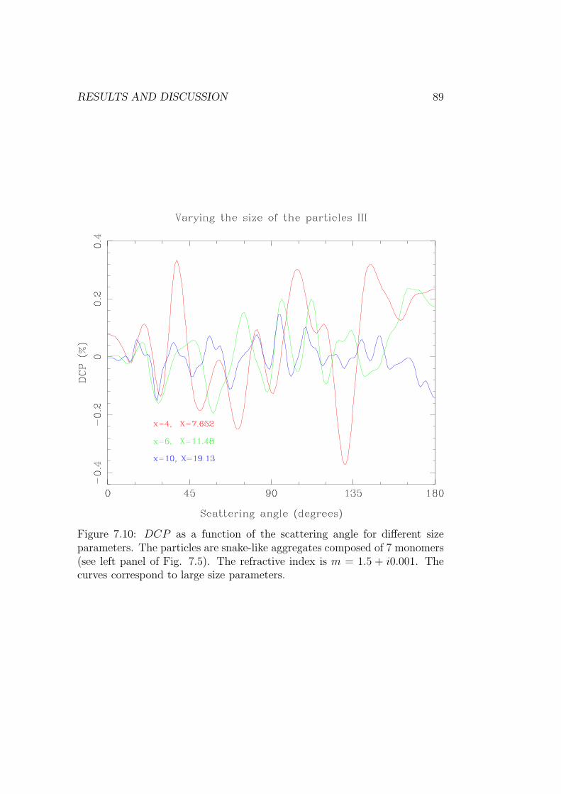
RESULTS AND DISCUSSION 89
Figure 7.10: DCP as a function of the scattering angle for different sizeparameters. The particles are snake-like aggregates composed of 7 monomers(see left panel of Fig. 7.5). The refractive index is m = 1.5 + i0.001. Thecurves correspond to large size parameters.

90 ASYMMETRICAL MODEL PARTICLES
Figure 7.11: DCP as a function of the scattering angle for a power-lawsize distribution of particles with exponent −3. The particles are snake-like aggregates made of seven monomers (see left panel of Fig. 7.5). Therefractive index is m = 1.5+i0.001. The computations were performed for 26sizes with req between 0.046 µm and 1.5 µm, with a wavelength λ = 0.5 µm.Most of the used sizes are placed in the range of small radii.

RESULTS AND DISCUSSION 91
Figure 7.12: DCP as a function of the scattering angle for different absorp-tions. The particles are snake-like aggregates composed of 7 monomers (seeleft panel of Fig. 7.5). The size parameter of the monomers that form theaggregate is x = 2 (X = 3.826), and the real part of the refractive index isfixed to Re(m) = 1.5.
refractive index. For this purpose, we considered samples made of only onekind of particles (regarding shape) of a fixed size. The particles are againsnake-like aggregates made of seven monomers (see left panel of Fig. 7.5).The size parameter of a monomer is x = 2, so X = 3.826. The real partof the refractive index is 1.5. We calculated the DCP as a function of thescattering angle for several values of the absorption, from Im(m) = 10−6 toIm(m) = 0.5. The curves for Im(m) smaller than 10−3 are not includedin Fig. 7.12, since they are very close to the curve for Im(m) = 10−3. Weconclude from Fig. 7.12 that the curves of the DCP tend to zero as theabsorption increases.
We also made some calculations for larger size parameters and we came

92 ASYMMETRICAL MODEL PARTICLES
Figure 7.13: DCP as a function of the scattering angle for different values ofthe real part of the refractive index. The particles are snake-like aggregatescomposed of 7 monomers (see left panel of Fig. 7.5). The size parameterof the monomers that form the aggregates is x = 2 (X = 3.826), and theimaginary part of the refractive index is fixed to Im(m) = 0.001.
to the same conclusion.
7.5.4 Changing the real part of the refractive index
Regarding the real part of the refractive index, we performed a study similarto that in Sec. 7.5.3. The imaginary part was fixed to Im(m) = 0.001, andthe real part varied from Re(m) = 1.2 to Re(m) = 1.8. The results areshown in Fig. 7.13. The behavior of the DCP in this case is exactly theopposite to that obtained by changing Im(m), i.e., the values of the DCPbecome generally larger (in absolute value) as the real part of the refractiveindex increases.

RESULTS AND DISCUSSION 93
When Re(m) tends to one, we enter the domain of Rayleigh-Gans scat-tering [68], where the DCP must get close to zero for all scattering angles.This might be an explanation for the behavior observed in Fig. 7.13.
7.5.5 Changing the number of monomers of an aggre-gate of constant size
In this section we start studying to what extent the exact shape of the par-ticles determines the shape of the curve of the DCP as a function of thescattering angle. As a first step, we analyzed the effect of changing the num-ber of component monomers of the aggregate, keeping the size of the wholeparticle constant. Again we took a snake-like shape, but this time the ag-gregates were composed of 4, 13, 16 and 25 monomers respectively (see Fig.7.14).
The size of the aggregates was X = 3.826 and we chose m = 1.5+ i0.001.The results (see Fig. 7.15) clearly tell us that the higher the number ofcomponent monomers is, the closer to zero the mean amplitude of the DCPbecomes. This behavior suggests that we would need aggregates made ofonly a few monomers to reproduce high values of DCP . We can also seein Fig. 7.15 how the complexity of the curves increases with the number ofmonomers.
A possible explanation for the results of this section may be the following.The peaks of the curves of the DCP are due to resonances in the interferenceof light after interacting with the asymmetrical particle. These resonanceslargely remain after averaging over all possible orientations. The numberof peaks of the curves of the DCP depends on the number of monomerscomposing the aggregate. Indeed, as the number of monomers of the particleincreases, the number of maxima and minima of the curves of the DCP alsoincreases. The scattering angle of the peaks and their amplitudes might bedetermined by the spatial distribution of the monomers in the aggregate andthe relation between the size of the monomers and the wavelength. In fact,the mean amplitude of the curves decreases as the monomers become smaller.This could be due to the fact that the optimal size-wavelength relation forthe resonance is lost.
7.5.6 Monomers of different sizes in the same aggre-
gate
So far, we have just used aggregates in which all constituent spheres havethe same size. It might be possible that the results we are obtaining are due

94 ASYMMETRICAL MODEL PARTICLES
Figure 7.14: Snake-like aggregates with different numbers of monomers. Thesize parameter is the same for all aggregates, so the size parameter of themonomers decreases as the number of monomers increases. Aggregates madeof 4, 13 16 and 25 monomers are shown.

RESULTS AND DISCUSSION 95
Figure 7.15: DCP as a function of the scattering angle for snake-like aggre-gates composed of different numbers of monomers (see Fig. 7.14). The sizeparameter of the aggregates is fixed to X = 3.826, and the refractive indexis m = 1.5 + i0.001.

96 ASYMMETRICAL MODEL PARTICLES
to that particular feature of the particles. In order to check this possibil-ity, we compared some of the results we already obtained with some othercalculations for particles formed by monomers of different sizes. We built aparticle made of monomers of tree different sizes, distributed as indicated inFig. 7.16. The volumes of the monomers are V0 ±∆V , where V0 is a certainreference volume, and ∆V is 0%, 10%, 20%, 30% and 50%. Note that allparticles have the same volume for the comparison to make sense.
Figure 7.16: Aggregate formed by 7 monomers of different sizes. There arespheres of tree volumes: V0, V0 + ∆V and V0 − ∆V , and the total volumeof the particle is the same as if the volume of all monomers of the aggregatewas V0.
In Fig. 7.17 we can see that there are not important differences (eitherqualitative or quantitative) between the results corresponding to ∆V = 0%,∆V = 10%, ∆V = 20% and ∆V = 30%. However, somewhere between∆V = 30% and ∆V = 50%, the DCP suddenly goes to zero for all scat-tering angles. An explanation might be that the observable features of theDCP curves are due to resonances that depend on relations between somesubstructures of the particles. For monomers with very different sizes thoserelations are not fulfilled and the resonances disappear. This result gives us acertain freedom in the configuration of the aggregate, allowing us to considermore realistic particles without loosing the high values for the DCP .

RESULTS AND DISCUSSION 97
Figure 7.17: DCP as a function of the scattering angle for snake-like ag-gregates made of differently-sized monomers (see Fig. 7.16). The size pa-rameter of the aggregates is fixed to X = 3.826, and the refractive index ism = 1.5+ i0.001. The percentages indicated in the legend are the differencesin volume among the monomers composing the aggregate.
7.5.7 Changing the shape
The last step is to change the shape by a completely different one, and com-pare the results with the ones coming from the snake-like shape for some sizes(Sec. 7.5.1). The new shape is that of the Mr Sanchez particle, described inthe right panel of Fig. 7.5. It is made of 25 identical homogeneous sphericalmonomers.
Figs. 7.18 and 7.19 show the results. In the first one we can see that forsmall size parameters Mr Sanchez produces in general a lower DCP than thesnake particle. However, for large sizes, the mean amplitude of the curves ofthe snake particle and Mr Sanchez are comparable, as shown in Fig. 7.19.
For a given size of the whole aggregate, the monomers composing Mr
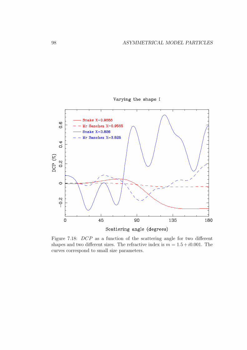
98 ASYMMETRICAL MODEL PARTICLES
Figure 7.18: DCP as a function of the scattering angle for two differentshapes and two different sizes. The refractive index is m = 1.5+ i0.001. Thecurves correspond to small size parameters.

RESULTS AND DISCUSSION 99
Figure 7.19: DCP as a function of the scattering angle for two differentshapes and two different sizes. The refractive index is m = 1.5+ i0.001. Thecurves correspond to large size parameters.

100 ASYMMETRICAL MODEL PARTICLES
Sanchez are substantially smaller than those of the snake-shaped particle.Consequently, if the argument posed in section 7.5.5 is valid, we should alwaysobtain a smaller amplitude for the curve of the DCP corresponding to MrSanchez than the one corresponding to the snake. However, the amplitudesare comparable for large size parameters. An explanation could be that forlarge sizes, the groups of monomers of Mr Sanchez, namely his head, hisarms and his legs work as a monomer of a size close to the optimal for theresonance.
This theory suggests that it might be possible to obtain large values ofthe DCP for samples of real particles if their shape is asymmetrical and thesubstructures responsible for the asymmetry are comparable in size to thewavelength.
7.6 Primary and secondary peaks
A common explanation to results given in Secs. 7.5.1, 7.5.2, 7.5.5, 7.5.6and 7.5.7 has been already suggested within the discussions correspondingto some of those sections. Nevertheless, we would like to summarize that inthe present section, and clearly define the concepts of primary and secondarypeaks, because they will be used in the next chapter.
While increasing the size of particles for a fixed wavelength, two importantfeatures appear in the curves of the DCP as a function of the scattering angle:
• When the size parameter of a grain rises over a certain limit Xp, thesubstructures of the particle that produce the asymmetry (groups ofmonomers), start to be non-negligible in size compared to the wave-length of the incident light. Then, some peaks (maxima and minima)appear in the curve: the primary peaks. Obviously, Xp is over the sizeparameters corresponding to the Rayleigh domain (see Sec. 3.6.2). Theprimary peaks are just a few, and both the number of them and thescattering angles they are located at, remain fixed when varying thesize of the particles. The amplitude of these peaks do change with thesize of the grains: it is maximum when an optimal ratio exists betweenthe size of the substructures that produce the asymmetry in a particleand the wavelength of the incident light, and decreases for smaller andlarger sizes.
• If we keep increasing the size of the grains up to a size parameterXs > Xp, other features appear in the curve: the secondary peaks.This happens when the size of the individual monomers becomes non-negligible compared to the wavelength. The number of these peaks
CONCLUSIONS 101
systematically increases while the size of the grains rises. The scatteringangles they correspond to, are not fixed, but they change with the sizeof the grains. The amplitude of the secondary peaks is maximum whenan optimal ratio exists between the size of the individual monomers ofan aggregate, and the wavelength. For the model particles studied inthe present chapter, the amplitudes of the secondary peaks are smallerthan those of the primary peaks.
Based on the above description, primary peaks seem to be due to reso-nances by the substructures of the particles that produce the asymmetry, andsecondary peaks seem to correspond to resonances between the monomers.
Primary and secondary peaks, as described above, are an explanation ofthe appearance and evolution of the different features of the curves of theDCP as a function of the scattering angle, while increasing the size of thegrains (Sec. 7.5.1). They also can explain the result of the size average inSec. 7.5.2: As the secondary peaks appear at different scattering angles fordifferent sizes, they vanish in the average when enough sizes are considered.On the contrary, primary peaks always appear at the same positions, so theyremain after adding the scattering matrices corresponding to different sizes.As for both the size average and the case of X = 2.678, the DCP curves areexclusively due to the primary peaks, the plot in Fig. 7.11 looks quite similarto the blue line of Fig 7.8: same number of peaks, with the same shape atthe same positions appear at both plots. Increasing the number of monomersof the snake-like particle in Sec. 7.5.5 makes the primary peaks to disappearbecause the optimal size ratio between the substructures that produce theasymmetry in the particle and the wavelength is lost. At the same time,more secondary peaks arise while more monomers are added to the particle,because new resonances appear. Using monomers of very different sizes toform the grains makes all resonances to disappear, so both, the primary andsecondary peaks vanish.
7.7 Conclusions
• For the snake-like shape with seven monomers and m = 1.5 + i0.001,the mean amplitude of the curve of the DCP is close to zero for smallsize parameters (as corresponds to the Rayleigh domain), and thengrows as the size parameters of the monomers increases to x = 1.8, inwhich case a maximum larger than 2% is found. When the size param-eter becomes larger than x = 1.8, the amplitude decreases gradually,becoming essentially zero for x = 10.

102 ASYMMETRICAL MODEL PARTICLES
• For the snake-like shape with seven monomers and m = 1.5+i0.001, thecomplexity of the curves of the DCP increases always when increasingthe size of the particle.
• Single scattering of optically inactive asymmetrical particles in randomorientations can give large values of the DCP of the scattered light(more than 2%), at least for a snake-like aggregate composed of sevenspherical monomers with m = 1.5 + i0.001.
• If we use a typical power-law size distribution, the curves of the DCPcorresponding to snake-like aggregates made of 7 monomers with m =1.5+i0.001 still show values of the DCP of the order of the observations(≈ 0.1% or less).
• Increasing the absorption of the particles makes the main amplitude ofthe curves of the DCP to decrease, at least for snake-like aggregatesof seven monomers with x = 2 and Re(m) = 1.5. However, the effectis the opposite if the imaginary part of the refractive index is fixed toIm(m) = 0.001 and the real part is increased.
• By increasing the number of monomers of an aggregate, but keeping thewhole size constant, the number of maxima and minima of DCP curvesincreases and the amplitudes of these decreases, at least for snake-likeparticles with x = 2 and m = 1.5 + i0.001.
• It is not necessary that monomers composing the aggregates are equal-sized to obtain high values of the DCP . In fact, the snake particlegives almost identical curves of the DCP even taking for the monomersvolumes as different as V0, V0 + 30%V0 and V0 − 30%V0.
• If the snake particle made of 7 monomers is compared to the MrSanchez particle (made of 25 monomers and more complex), the meanamplitude of the curve of the DCP is larger for the snake at small sizeparameters (X . 4), but it is comparable for both shapes if the size ofthe aggregates is large enough (X & 7).
• The peaks of the curves of the DCP may be due to resonances. Thereexist two types of peaks: primary peaks (fixed number, at fixed scat-tering angles and due to resonances by the substructures that producethe asymmetry of the particle), and secondary peaks (the number in-creases with the size of the grain, not at fixed scattering angles and dueto resonances by the monomers).

Chapter 8
Circular polarization of lightscattered by irregular particles
Some of the results included in this chapter were published in [23] and presented in the X
Conference on Electromagnetic & Light Scattering by Non-Spherical Particles.
Abstract
A collection of irregular aggregates of identical spheres was built by usinga Monte Carlo implementation of a cluster-cluster aggregation model. Thebehavior of the DCP as a function of the scattering angle was studied forthose particles. After averaging over a few sizes and shapes, the DCP rapidlytended to zero, so we deduced that the asymmetry of the particles cannotaccount for the observed DCP in comets.
8.1 Introduction
The results of the previous chapter did not definitively rule out the asym-metry of randomly oriented particles as the responsible mechanism of theobserved DCP in comets, because the calculated values of the DCP werecomparable to the observations, even when averaging over sizes for a specificmodel shape. As a consequence, a study regarding a collection of irregu-larly shaped particles must be carried out. It is obvious that averaging overa large number of randomly irregularly shaped particles will finally yield azero DCP , because there will be always a particle similar to the mirror par-ticle of some other, so mirror symmetry will be achieved in the sample. Inthe present chapter, we are not questioning this fact, but we are trying toasses how many different shapes are needed to obtain a asymthotic behaviorof the DCP towards zero. For instance, if twenty or fifty different shapes
103
104 IRREGULAR PARTICLES
are enough, we can inmediately disregard this mechanism, but if a numberlarger than present in a comet is needed, the asymmetry of particles wouldmake a significant contribution to the DCP of light scattered in comets.
8.2 Building the aggregates1
We again work with aggregates of identical spheres as in the previous chapter,because calculations of the scattering matrix of such particles is fast andaccurate by using the T-matrix method along with the superposition theorem(see Sec. 7.4).
For the generation of the aggregates, we made a Fortran implementationof both a particle-cluster aggregation (PCA) and a cluster-cluster aggregation(CCA) Monte Carlo methods. The PCA process starts with a single spherein a fixed position (see the upper part of Fig. 8.1). A new sphere is thenattached to it in a random direction. From then on, the procedure consistsof adding a new sphere to any of the previously added in a random direction.Then, it must be checked that the new monomer does not overlap with any ofthe others. If it does, the last aggregated sphere has to be removed, and a newattempt to aggregate a non-overlapping monomer is performed. For CCA,several PCA clusters are built first, and then they are joined together (seethe lower part of Fig. 8.1). We stick them together in the following way: weset one of the clusters in the origin, and we put another one far away from thefirst (in such a way that they do not overlap), in a random direction. Then wemake the second cluster to approach the part of the aggregate that is alreadyformed, until both parts get in touch. For both PCA and CCA methods, thecoagulation process finished when the maximum distance between any pairof monomers of the aggregate exceeds a certain upper limit (dc for PCAand dp for CCA). This criterion is realistic, because the actual limitationin the size of an aggregate is given by the maximum length of the particle:the larger this length is, the stronger the centrifugal force may become forthe monomers at the edge. As the forces sticking together the monomers isconstant, aggregates are broken as a consequence of their rotation when theyexceed a certain size.
After building some random aggregates by both of these methods, wemade some preliminar calculations of the DCP derived from single scatter-ing by these particles in random orientation. We found that CCA clusters
1The cluster-cluster aggregation model presented in this section was included in thepeer-reviewed paper by R. Vilaplana, J. Canto, F. Moreno and D. Guirado entitled The in-
fluence of particle shapes and sizes in the CO ice stretching mode, accepted for publicationin Earth, Planets and Space in 2009 [69].

NUMERICAL METHOD 105
Figure 8.1: Models of aggregation to build the particles. For PCA, identicalmonomers are sticked together sequentially to the particle until the maximumdistance between two monomers is larger than a certain limit dc. For CCA,several PCA aggregates a joined together until the maxium distance betweentwo monomers of the particle becomes larger than dp.
give higher values of the DCP , which makes sense, because CCA producesaggregates with elongated substructures, which is favourable to the asym-metry of the formed particles. Fig. 8.2 shows the difference between a PCAand a CCA generated aggregate.
According to this, only CCA aggregates were considered for the rest ofthis chapter. Some of the generated CCA shapes used for calculations inSecs. 8.5 and 8.6 are shown in Fig. 8.5.
8.3 Description and validation of the numer-
ical method
As we already stated in Sec. 7.4, the implementation of the T-matrix tech-nique by Mackowski & Mishchenko [42] is the best choice for our calculations.Since only some checks for model particles have been performed on the codeso far (see Sec. 7.4), we add at this point some comparisons between the re-sults given by Mackowski & Mishchenko’s T-matrix and Draine’s DDA [17]for randomly built (irregular) grains. We made calculations for the threeaggregates shown if Fig. 8.4. A silicate-like refractive index was set for thegrains (Im(m) = 1.5+i0.001), for the same reasons as in the previous chapter(see Sec. 7.4).

106 IRREGULAR PARTICLES
Results on the DCP as a function of the scattering angle are shown inFig. 8.5. A satisfactory agreement between both methods was found.
To assure the accuracy of the calculations, we adopted two aditional cri-teria:
• Checking that all calculated scattering matrices fulfill the coherencytest (see Sec. 3.6.3).
• Imposing the same criterion for stability of the calculations as in theprevious chapter (see Sec. 7.4).
8.4 Some examples for individual particles
Let us take any of the generated irregular aggregates, for instance, the oneshown in Fig. 8.6. We calculated the DCP of light scattered by this particlein random orientation as a function of the scattering angle for m = 1.5 +i0.001. Results for several sizes of the particle are shown in Fig. 8.7. Wefound a number of features in this plot, that we compared to the thosecorresponding to the snake-like model particle given in Fig. 7.2:
Figure 8.2: Two examples of randomly built aggregates. The particle on theleft side is formed by 151 monomers, and it was constructed by the PCAmethod. The one on the right side is a CCA aggregate composed of 145monomers. It is clear that PCA aggregates are more compact and close to asymmetrically shaped particle than CCA. CCA particles are more likely tobe asymmetrical.

INDIVIDUAL PARTICLES 107
Figure 8.3: Some of the generated CCA clusters that were used for calcula-tions of the DCP .
• At small sizes, the primary peaks appear for the irregular particle aswell as for the model particle (see Fig. 7.8). It happens because thelight starts distinguishing the substructures of the aggregate (groups ofmonomers) that produce the asymmetry, i.e., the size of such structuresbecomes not negligible compared to the wavelength of the incominglight.
• For larger sizes, the primary peaks increase their amplitude as in thecase of the model grains (Fig. 7.9). The reason is that the size ofthe substructures producing the asymmetry of the particle becomescomparable to the wavelength.

108 IRREGULAR PARTICLES
• The secondary peaks arise for larger values of the size parameter, as inthe model particle (Fig. 7.10). We explained this fact by assuming thatfor these sizes, the radius of the monomers is not negligible comparedto the wavelength (light starts to distinguish the individual monomersof the particle, so a lot of resonances appear).
• All the above features are similarities between the DCP given by asym-metrical model particles and irregular scatterers. The difference is that,contrary to model aggregates, for irregular particles the primary peakshave smaller amplitude than the secondary. This may be due to the factthat the substructures producing the asymmetry are not as noticeablein the irregular particles as they were in the model grains.
8.5 Averaging over sizes for individual shapes
As in Sec. 7.5.2, we assumed a power-law size distribution of particles withan exponent −3. We considered one shape at a time and performed thesize average of the scattering matrix of particles of that shape in random
Figure 8.4: Three irregular aggregates of identical spheres. The size param-eter of the monomers is x = 0.26 for all cases. Aggregate (a) is made of 93monomers, so the size parameter of the whole particle is X = 1.19. For (b),the number of monomers is 96, what yields X = 1.20. Particle (c) has a sizeparameter of X = 1.14 because it is made of 83 monomers.

SIZE AVERAGE 109
Figure 8.5: Comparison of Mackowski & Mishchenko’s T-matrix code resultswith Draine’s DDA calculations for the three irregular aggregates of identicalspheres plotted in Fig 8.4.
Figure 8.6: Randomly built CCA particle made of 93 identical monomers.

110 IRREGULAR PARTICLES
Figure 8.7: The DCP as a function of the scattering angle for particle givenin Fig. 8.6. Three size parameters were considered for the same shape. Therefractive index is set to m = 1.5 + i0.001.
orientation. In order to perform an adequate sampling of the chosen sizedistribution (power-law), we needed to consider a relatively larger amount ofparticles in the lower size limit than in the upper size limit, as the power-lawfunction changes very rapidly for small sizes. Thus, we chose thirteen differ-ent monomer size parameters x as follows: : 0.21, 0.22, 0.24, 0.26, 0.29, 0.31,0.35, 0.39, 0.45, 0.52, 0.63. 0.79 and 1.05. The size parameter of an aggregatemade of NMON monomers can be calculated as X = (NMON)1/3x.
A representative example of the result after performing the average isgiven in Fig. 8.8. It corresponds to the particle shown in Fig. 8.6, withm = 1.5 + i0.001. The general appearance of the resulting curve is thatof the primary peaks: they appear because they are always located at thesame scattering angles and because they are produced by small particles,which have a larger weight in the average according to the power-law size

SIZE AVERAGE 111
distribution. There is a little distorsion by the secondary peaks in the caseof randomly built aggregates because for this case they have a larger ampli-tude than the primary ones. But they still do appear at varying scatteringangles depending on the size of the aggregate, so they should not make anycontribution to an average with a sufficiently high number of sizes samplingthe size distribution. When the secondary peaks dissapear, only the primarypeaks (with a small amplitude compared to model particles), remain. Thismeans that randomly built aggregates averaged over sizes for a fixed shapeproduce a lower DCP that the model particles of Fig. 7.5.
Size averages were calculated for twelve different shapes. Table 8.1 showsthe maximum DCP (in absolute value) obtained for each average.
Figure 8.8: Average of the DCP as a function of the scattering angle, overthirteen sizes, all of them corresponding to the same particle shown in Fig.8.6. The refractive index was set to m = 1.5 + i0.001.

112 IRREGULAR PARTICLES
Aggregate max |DCP | (%)CCA1 0.083CCA2 0.056CCA3 0.308CCA4 0.061CCA5 0.082CCA6 0.035CCA7 0.170CCA8 0.085CCA9 0.106CCA10 0.093CCA11 0.094CCA12 0.088
Table 8.1: Maximum values of the DCP as a function of the scattering angle,obtained by size averages of twelve individual different shapes.
8.6 Averaging over shapes the size averages
Results on the effect of averaging over 12 shapes the sizes averages are plottedin Fig. 8.9. Averaging the DCP curves over a number of shapes rapidlyleads to zero values of the DCP because the primary peaks are located atdifferent scattering angles for different shapes, so no constructive additionis made when workin with the shape-averaged sample. According to this,single scattering by randomly oriented irregular particles must be ruled outas the responsible mechanism of the observed DCP in comets.
8.7 Conclusions
• Primary peaks have smaller amplitudes in randomly built aggregatesthan in the asymmetrical model particles used in the previous chapter.
• Secondary peaks have larger amplitudes than primary ones in randomlybuilt aggregates.
• The DCP of a sample of particles averaged over sizes for a fixed shapeis mainly determined by the primary peaks, as in the case of modelparticles.
• A lower DCP arises from a size-averaged sample of randomly builtaggregates of a fixed shape than for that of model grains.

CONCLUSIONS 113
• The DCP rapidly tends to zero when building a sample with just afew size-averaged shapes.
• Single scattering by asymmetrical particles in random orientation doesnot make a significant contribution of the observed DCP in comets.
Figure 8.9: DCP as a function of the scattering angle for a sample averagedover twelve shapes, each one averaged over thirteen sizes.


Chapter 9
Circular polarization of lightscattered by optically activematerials
Although all studies reveal that optically active materials are not the maincomponents of cometary dust, they must be carefully considered, because asmall percentage of those materials in the composition of dust grains couldbe enough to circularly polarize the scattered light significantly.
Regarding mineral particles, searching for optically active materials meanssearching for crystalline minerals with a non-symmetric christalization sys-tem, as previously stated in Sec. 5.3. The only information we could obtainabout such materials in comets, is given by Min et al. [48]: they deduced avolume abundance of 1.3% of chrystalline enstatite in Comet Hale-Bopp. En-statite usually chrystallizes in the orthorrombic system, but at temperaturesas low as those prevailing in cometary environments, it might be presentin form of monoclinic chrystals, which are asymmetrical, so that they cancircularly polarize light.
Organic materials [65], and in particular some amines [21], were found atvery low abundances in the collected particles of Comet Wild 2 by Stardustmission. Some of these amines are optically active.
As explained above, there exist evidences that optically active materialsare present in comets. Hence, the relevant question at this point is whetherthey are abundant enough to produce a DCP on the scattered light compa-rable to the observed. We decided not no initiate such an analysis, becausethe mechanism of optical activity do not match with the main features ofthe observations that we enumerated in Sec. 4.3: if optically active materi-als are present in cometary comae, in principle there is no reason to thinkthat the distribution of them inside the coma is not homogeneous (in relative
115

116 OPTICAL ACTIVITY
abundance). If it is homogeneous, it makes no sense that the observed DCPdecreases when increasing the aperture of the diaphragm, and there is noreason for the DCP to tend to zero in the vicinity of the nucleus. Accordingto this, we decided to directly rule out this mechanism without any furtherconsideration.
Nevertheless, we would like to remark that some authors claim that theobserved DCP in comets has a predominant sign (see, e.g., [61]). Eachoptically active substance polarizes light always in the same sense, so theocurrence of a predominant sense of CP would support the idea that the op-tical activity is the responsible for the observed DCP in comets. Rosenbushet al. [63] obtained only negative values of the DCP for different regions ofthe coma of Comet Hale-Bopp at a phase angle of 46. Manset & Bastien[43] observed mainly negative values as well for the same comet, the phaseangle varying from 47.4 to 40.0. However, we would like to point out thatobservations at one single phase angle, or in a very narrow range of them, arenot enough to assure that the CP has a predominant sense in a comet. Theremight be some dependence of the DCP on the phase angle. In fact, CometC/1999 S4 (LINEAR) was observed by Rosenbush et al. [61] for eight phaseangles varying from 60.9 to 122.1, and it is clear from the plots presentedin the paper, that the DCP is mainly possitive for the smallest phase angle,and then it progressively changes to negative as the phase angle increases.In conclusion, the predominant sign of the DCP in a comet could be due toa phase angle dependence.

Chapter 10
Monte Carlo model of radiativetransfer in comets
Some results on the radiative transfer model described in the present chapter were pub-
lished in [24] and presented in three conferences: 41st annual meeting of the Division
for Planetary Sciences of the American Astronomical Society (oral presentation), the 10th
Asteroids, Comets, Meteors meeting (poster presentation) and the XI Conference on Elec-
tromagnetic & Light Scattering by Non-Spherical Particles (oral presentation).
Abstract
A Monte Carlo model of radiative transfer in comets has been developed.It calculates the four Stokes parameters of the light scattered by particlesin the coma, assuming a certain distribution of the grains around a spheri-cal nucleus. By applying this model, non-negligible values of the DCP wereobtained just by assuming conditions of multiple scattering by spherical opti-cally inactive particles, and considering only light coming from a non centralsmall region of the coma of the comet, an asymmetrical distribution of dustin the coma, or both. Nevertheless, these values are one or two orders ofmagnitude below the observed, at least for silicate-like spherical particles.
10.1 Introduction
We have already analyzed all mechanisms regarding the particles of cometarycomae that are candidates to circularly polarize light. For none of thosemechanisms was necessary to consider the structure of the comet (a nucleusand a certain distribution of particles in the coma). For the aligned particles(Chap. 6), it was enough to consider a single grain, to calculate how it isaligned and finally deduce that no CP could arise from grains that are aligned
117

118 RADIATIVE TRANSFER MODEL
that way. In Chaps. 7 and 8 we just had to calculate averaged scatteringmatrices of different ensembles of particles. To study the rest of the proposedmechanisms in Sec. 5.4, it is necessary to consider the whole structure ofthe comet: size and albedo of the nucleus, number density distribution ofdust particles in the coma, etc. Our model must account for facts like theinteraction of photons with the nucleus, the possibility of multiple scatteringof a photon before it escapes from the comet and the possibility to observelight coming from a small region of the comet.
Available options for modelling were the the doubling adding method [28]and a Monte Carlo model. The doubling adding thecnique is not suitablefor our study because it is meant for plane-parallel atmospheres. We couldhave made the approximation of local plane-parallel atmosphere in a comet,but that would not have permitted us to investigate the effects of the actualstructure of the comet on the scattered light. Therefore, we chose the MonteCarlo technique. Our Monte Carlo model consist of launching photons intoa certain target, tracking their evolution until they are extinguished, andrecording all contributions they make to the outgoing light. Although largecomputational resources (especially computational time) are needed to runMonte Carlo codes, they are the most exact models to reproduce a real radia-tive transfer process. New multicore desktop computers offer the possibilityof easily reaching statistical stability of the results of a Monte Carlo code ina reasonably short computational time. We think that Monte Carlo modelsshould become the first option for modelling atmospheres in the near future.
There exist, at least, two previous approaches to the Monte Carlo mod-elling of radiative transfer in comets. The first one was developed by Saloin 1988 [64]. It consists of a model to compute the incoming energy to thenucleus of a comet, considering external solar radiation and internal infraredthermal re-radiation by the particles in the coma. The second one was devel-oped by Moreno et al. in 2002 [53], and it deals with the outgoing radiationof comets when illuminated by the Sun. Althoug this model calculates thefour Stokes parameters of light scattered in the comet, only results on theflux and EDLP were presented, and no results were given on the DCP .
In this chapter, we present a similar model to that by Moreno et al., im-plemented in a new code built from the begining with better routines andnumerical methods in order to improve the accuracy of the results and toreduce the computational time to achieve statistical stability. These im-provements are necessary to get reliable results concerning CP , because, asseen in Chap. 4, we expect the calculated DCP to be close to zero.

MULTIPLE SCATTERING 119
10.2 Multiple scattering as a mechanism to
produce circular polarization on a single
photon
Let us consider one single photon of natural light singly scattered by a sampleof particles fulfilling both the reciprocity and mirror symmetry conditions.The initial Stokes vector of the photon is proportional to (1, 0, 0, 0)t, andmultiplying this vector by the scattering matrix of the sample (Eq. 3.90)gives us the Stokes parameters of the scattered photon, which is proportionalto (F11, F12, 0, 0)t. The DCP of the singly scattered photon is zero, becausethe last Stokes parameter Vsca is null (see definition in Eq. 3.56). It doesnot matter how many photons compose the incident light beam, after addingthe Stokes vectors of all photons scattered in a certain direction (all withVsca = 0), the DCP of the integrated light will be zero. This means that inconditions of single scattering, it is not possible to achieve any DCP even inthe case that the system is asymmetrical around the direction of the incidentlight. This statement works as an example of the fact that the condition forCP given in 5.2 is just necessary, but not sufficient.
Nevertheless, multiple scattering can circularly polarize a single photon.The proof is simple: in the second scattering event, the scattering planechanges, so the Stokes parameters of the singly scattered photon must betransformed according to Eq. 3.59. After rotating the scattering plane by anangle irot, (F11, F12, 0, 0)t becomes (F11, F12 cos 2irot,−F12 sin 2irot, 0)t. Stillthe DCP is zero, as expected because I and V do not depend on the planeof reference (Sec. 3.3). Multiplying the new Stokes vector by the scatteringmatrix leads to:
(F 211+F 2
12 cos 2irot, F11F12+F22F12 cos 2irot,−F12F33 sin 2irot, F12F34 sin 2irot)t.
Thus, the DCP of a single photon may be different from zero after twoscattering events.
Based on the last discussion, we have now two necessary conditions fora comet to produce CP if the particles forming its coma are symmetrical,optically inactive and randomly oriented:
• The part of the comet we are observing must be rotationally asymmet-rical around the direction of the incident light.
• There must be some multiple scattering.

120 RADIATIVE TRANSFER MODEL
10.3 Description of the model
Let us represent a comet by a spherical cloud of dust with a spherical solidshell of radius RN in its center (see Fig. 10.1). The cloud extends to theinfinity but its particle number density distribution varies as 1
r2 with the dis-tance r to the center of the system. Suppose that the relative abundances ofparticles of each size is the same at all volume elements dV . This is called thehypothesis of homogeneous coma, but it does not mean that the coma is ho-mogeneous, because the number density of particles may be different at eachpart. The cloud is illuminated from a far distance by a plane-parallel sourcemuch wider than the solid nucleus. Photons of natural light are launchedfrom the source, their paths are tracked and when they escape to the infin-ity, their Stokes parameters are transformed into spherical coordinates andfinally recorded along with the direction (θ, ϕ) of escape (see Fig. 10.1). Inthis way, a complete map of the Stokes parameters can be obtained by addingthe Stokes vectors of those photons escaping in a given direction.
The system of reference used along the present chapter is also defined inFig. 10.1.
10.3.1 The particles of the coma
As we studied in Chaps. 6 to 9, there exist several mechanisms by whichparticles may produce some DCP on the scattered light under certain con-ditions. Since we did not want them to mix up with the multiple scatteringby an asymmetrical comet, we assumed spherical optically inactive particlesfor the coma. We calculated the scattering matrices of the grains by usingBohren & Huffman’s implementation of the Mie theory [3]. However, wemust note that the versatility of the model allows us to use any type of par-ticles. An average scattering matrix over a size distribution was calculatedin all cases, and that is the matrix we used for every single scattering event.This represents a real case in conditions of single scattering (see Sec. 3.6),but if multiple scattering arises, it is just an approximation. The correctoption would be to use a different scattering matrix for each sphere size, anduse the size distribution to decide which one to use for each scattering event.However, this would make the code much slower, so we decided to use theapproximation of average scattering matrix, even in conditions of multiplescattering.
It is important to remark that for non-spherical grains in the coma, theorientation average is also valid only for single scattering conditions. A scat-tering matrix of all particles at each orientation should be calculated, and oneof them should be used at each scattering event for an exact representation
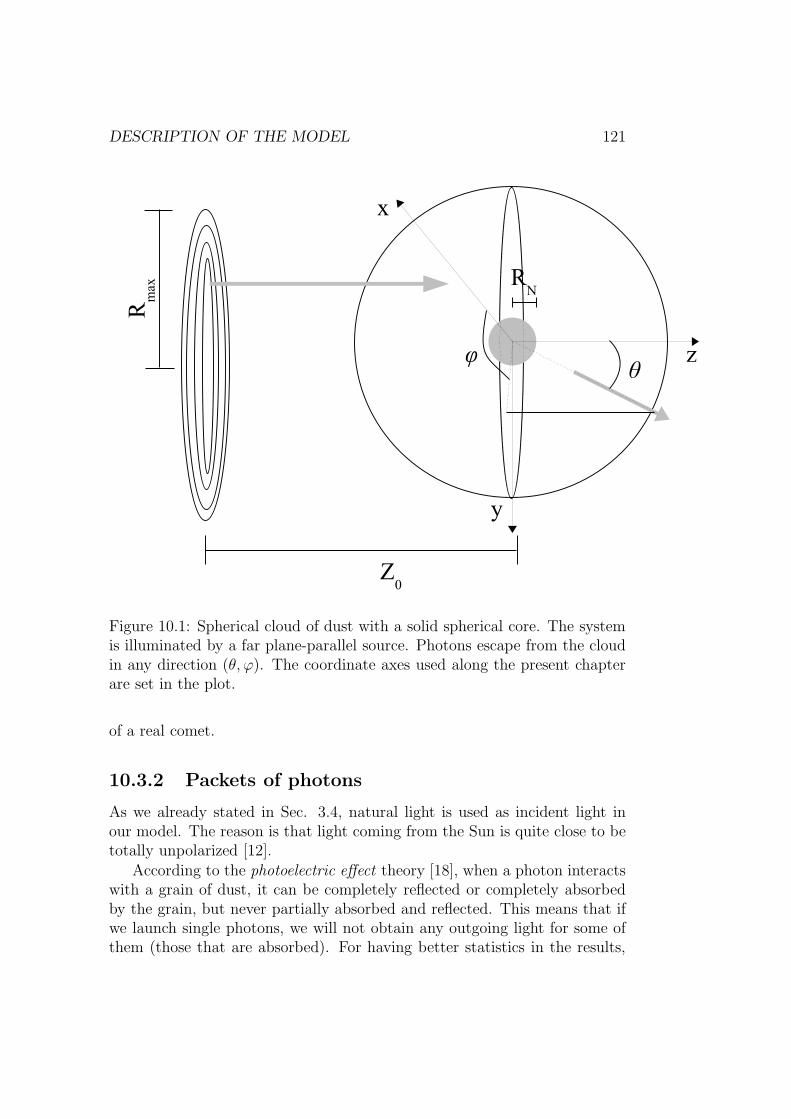
DESCRIPTION OF THE MODEL 121
Figure 10.1: Spherical cloud of dust with a solid spherical core. The systemis illuminated by a far plane-parallel source. Photons escape from the cloudin any direction (θ, ϕ). The coordinate axes used along the present chapterare set in the plot.
of a real comet.
10.3.2 Packets of photons
As we already stated in Sec. 3.4, natural light is used as incident light inour model. The reason is that light coming from the Sun is quite close to betotally unpolarized [12].
According to the photoelectric effect theory [18], when a photon interactswith a grain of dust, it can be completely reflected or completely absorbedby the grain, but never partially absorbed and reflected. This means that ifwe launch single photons, we will not obtain any outgoing light for some ofthem (those that are absorbed). For having better statistics in the results,

122 RADIATIVE TRANSFER MODEL
it would be desirable to get several outgoing light recorded events for eachlaunch. There is a way to do this: launching packets of photons. Packets arecollections of photons travelling together. We call the weight of the packetW to the proportion of the initial quantity of photons that still remains inthe packet after a number of interaction events. Obviously, the initial weightof any packet is W = 1. We do not have to decide whether a packet isabsorbed or reflected by a particle: a part of it is absorbed and the rest isreflected according to the single scattering albedo. In the same way, a part ofthe packet interacts with grains, while the rest goes to the infinity or to thenucleus, according to the probability of interaction with particles (given bythe optical depth of the path ahead of the packet). The weight of a packetof photons is reduced each time that a part of it goes to the infinity or tothe nucleus, and after each scattering event (see Sec. 10.3.4 for a detailedexplanation). We track the evolution of packets until they vanish. We willconsider that a packet is extinguished when its weight becomes lower than acertain limit Wmin.
The Sun is so far from comets that the wave front reaching a comet isplane, and photons do not interact with the grains of the coma until theyare very close to the comet. To reproduce these facts, we set a plane sourceof packets of photons at a distance Z0 from the center of the comet (see Fig.10.1). To ensure that the source is far enough, we checked that the results ofthe model are the same by using a distance Z0 as by considering 2Z0. We setthe launching platform circular with radius Rmax (Rmax ≫ RN). To ensurewe chose a correct value of Rmax we performed the same test as for Z0. Tomake the flux uniform, as in the Sun, we did the following: Let us call ρ thedistance from the launching point to the center of the launching platform (seeFig. 10.2), and PL the probability of a packet of photons to be launched froma point within [ρ, ρ + dρ]. If we denote by pL the corresponding probabilitydensity function, PL(ρ) = pL(ρ)dρ. If we divide the launching disk into smallrings, the uniform-flux condition means that the probability of a packet to belaunched from a specific ring must be proportional to the surface of that ring.Assuming infinitesimal rings, this leads to PL(ρ) ∝ ρdρ, since the surface ofan infinitesimal ring is dS = 2πρdρ. As a consequence pL(ρ) ∝ ρ. We canobtain the constant that we need to make this an identity by applying thenormalization condition
∫ Rmax
0pL(ρ)dρ = 1. The result is:
pL(ρ) =2ρ
R2max
. (10.1)
The probability density given by Eq. 10.1, along with the probability distri-bution sampling method described in Appendix A, easily lead us to a formula

DESCRIPTION OF THE MODEL 123
for sampling values of the initial ρ coordinate of the launched packets:
ρ =√
ξRmax, (10.2)
where ξ is a random number uniformly distributed within [0, 1].In order to improve the statistical stability of the model, we divided the
launching disk into NRING rings of equal surface (see Fig. 10.2), and welaunched one packet of photons from each ring, starting from the central ring(actually a circle) and moving to the border sequentially. In this way it isassured that packets are launched from all regions of the launching platform.As rings have a certain width, the exact value of ρ for a packet to be launched
Figure 10.2: The launching disk is divided into a number of rings of equalarea (as many as launched packets). Then, one packet is launched from eachring. For the inner rings, each packet is split into a number of sub-packets,and each of them is launched from a different point [ρ, ϕ] into the ring. Theexact coordinate ρ that a sub-packet is launched from, is calculated in sucha way that the number of photons launched per unit area remains constant.Coordinate ϕ is uniformly randomly distributed in [0, 2π].
from a certain ring [ρ1, ρ2] is obtained through the distribution given by Eq.
124 RADIATIVE TRANSFER MODEL
10.1 and the method described in Appendix A as follows:
ρ = ρ1 +√
ξ(ρ22 − ρ2
1). (10.3)
The angle ϕ (see Figs. 10.2 and 10.1) can be obtained as a uniformly dis-tributed random number within [0, 2π].
A last issue to consider regarding the sampling of the launching coordi-nates is that it is important to resolve the central zone of the launching diskbetter than the outer part, in order to correctly account for the interactionof light with the nucleus. If the central ring covers a zone wider than thenucleus, then only one packet will be launched directly to it, and just a fewof them will be deviated into it from a nearby region. Hence, there will notbe good statistics for the incoming light on the nucleus, which is importantbecause the interaction of light with the nucleus affects the outgoing radi-ation. The solution we adopted was to divide the launching platform into3 zones: a)ρ ≤ RN , b)RN < ρ ≤ 10RN , and c)10RN < ρ ≤ Rmax, withndiv1 > ndiv2 > ndiv3. In zone a), ndiv1 sub-packets of weigh W = 1
ndiv1
arelaunched instead of one only packet of W = 1. In region b) the division ofthe packet is by ndiv2 and in region c) by ndiv3. When several sub-packetsare launched from the same ring, a different ρ and a different ϕ are sampledfor each of them.
10.3.3 Interaction of a packet of photons with the grains
Let Φ be the flux of the incoming light, and let us call σ the average scatteringcross-section of all particles in a certain volume element dV . Then, by thedefinition of the scattering cross-section (see Sec. 3.1), the decrease of theflux for light traveling a distance ds through dV is given by:
dΦ = −Φnσdl, (10.4)
where n is the particles number density in dV . By integrating, we obtain theexponential decay law :
Φ = Φ0e−τ , (10.5)
where τ =∫ s
0nσds′ is called the optical depth. It is a dimensionless magni-
tude. Suppose that n is the same at all points of the cloud (which is not thecase along the present study). Then, the mean free path of photons, whichis defined as
∫∞0
nσe−τsds, would be 1nσ
, and τ = nσs. Therefore, in thecase of n to be constant, the optical depth can be understood as the distancemeasured in units of the mean free path, i.e., it gives an idea of whethera photon is going to interact with particles when crossing a cloud or not.

DESCRIPTION OF THE MODEL 125
This is why it is usually interpreted that a cloud of particles with τ > 1 isopaque, and it is translucent if τ < 1. We will call optical thickness to theoptical depth of the whole object, like a comet or a gas cloud. As the relationbetween the optical depth and the distance is not linear, the optical depthmay be finite for an infinite distance (for example, if σ is constant and thenumber density changes as 1
s2 along the path to the infinity).The probability density of interaction of the packet of photons with a
grain is:
p(s) =d(1 − Φ
Φ0
)
ds= nσe−τ , (10.6)
which means that the proportion of photons that interact with particleswithin [s, s + ds] is p(s)ds ∝ nσe−τds. Equivalently, the proportion of pho-tons that interact with particles within [τ, τ +dτ ] is p(τ) ∝ e−τdτ . Let us callτmax the maximum optical depth that a photon may travel (optical depth tothe infinity or to any obstacle). The normalization constant a1 of p(τ) canbe obtained from the normalization condition:
∫ τmax
0
a1e−τdτ = 1 ⇔ a1 =
1
1 − e−τmax⇒ p(τ) =
e−τ
1 − e−τmax. (10.7)
Once the probability density function has been derived, we can apply thegeneral sampling method by using uniform random numbers (see AppendixA):
ξ =
∫ τ
0
e−τ ′
1 − e−τmaxdτ ′ ⇔ τ = − ln[1 − ξ(1 − e−τmax)]. (10.8)
Let us now calculate the formula to translate physical distance to opticaldepth and vice versa. As we made the homogeneous coma hypothesis (Sec.10.3), σ is constant in the cloud, so we can write:
τ =
∫ s
0
σn(s′)ds′ = σ
∫ s
0
n(s′)ds′. (10.9)
To proceed, we need to assume some particular number distribution of grainsin the coma. For simplicity, we chose n(r) = a2
1r2 , with a2 = constant. Let
us call τN the optical depth of the whole cloud from the surface of the nucleusto the infinity in the radial direction. Then:
τN =
∫ ∞
RN
σn(r)dr = a2σ
∫ ∞
RN
dr
r2⇒ a2 =
τNRN
σ. (10.10)
By substituting a2 in Eq. 10.9 we obtain:
τ = τNRN
∫ s
0
1
r−2ds′. (10.11)

126 RADIATIVE TRANSFER MODEL
Figure 10.3: Initial (r0) and final (r) positions of a packet of photons. Thedistance travelled in the direction of propagation e is denoted by s. A non-right triangle is formed by edges r, r0 and s, that can be solved by the lawof cosines.
The radial distance r is different from the distance s if the path of thepacket of photon is in a non-radial direction. In Fig. 10.3 it is clear that theproblem can be easily solved by the well-known law of cosines as follows:
r2 = s2 + r20 − 2sr0 cos α. (10.12)
As r0 · e = −r0 cos α,r2 = s2 + r2
0 + 2sr0 · e. (10.13)
Combining Eqs. 10.13 and 10.11 leads to:
τ = τNRN
∫ s
0
(r20 + 2s′r0 · e + s′2)ds′. (10.14)
By solving the integral in Eq. 10.14, we get:
τ =τNRN
∆
(
arctanr0 · e + s
∆− arctan
r0 · e
∆
)
, (10.15)
if ∆ =√
r20 − (r0 · e)2 6= 0.
In the particular case that s → ∞, we just calculate the limit in Eq.10.15:
τ∞ =τNRN
∆
(
π
2− arctan
r0 · e
∆
)
. (10.16)
We can obtain s as a function of τ just by working its value out in Eq.10.15 :
s = ∆ tan∆τ
τNRN+ arctan
r0 · e
∆− r0 · e. (10.17)

DESCRIPTION OF THE MODEL 127
In the case that ∆ ≈ 0, we may have some numerical problems in applyingEqs. 10.15 to 10.17. Having ∆ ≈ 0 means that r0 ≈ r0 · e, i.e., r0 is almostparallel (or anti-parallel) to e. This happens to packets of photons launchedfrom the central region of the launching platform, before they interact withany grain. The solution to this numerical issue is to build the equationsfor the special case ∆ = 0, and use them when the actual ∆ is below acertain minimum value ∆min. Let us go back to Eq. 10.14. There exist twopossibilities for ∆ = 0:
• r0 ‖ e in the opposite sense (r0 · e = −r0): packets of photons cominginto the nucleus in radial direction.
• r0 ‖ e in the same sense (r0 · e = r0): packets of photons travelling faraway from the nucleus in radial direction.
For packets of photons approaching the nucleus:
τ = −τNRNs
r0(s − r0), (10.18)
and for those moving far away from the nucleus:
τ = τNRNs
r0(s + r0). (10.19)
For the particular case that the packet goes to the infinity, we just calcu-late the limit s → ∞ in Eq. 10.19:
τ∞ =τNRN
r0. (10.20)
Now we work s out from Eqs. 10.18 and 10.19. For packets of photonsapproaching the nucleus:
s =τr2
0
τNRN + τr0, (10.21)
and for those travelling far away from the nucleus:
s =τr2
0
τNRN − τr0. (10.22)
For obtaining the optical depth to the nucleus τc, we just have to applyEq. 10.15 if ∆ > ∆min or Eq. 10.18 if ∆ ≤ ∆min, but in all cases we need thedistance to the nucleus sc. Let us call now r0 the position vector of a packetof photons that points in the direction (and sense) of the unit vector e. Fig.10.4 shows a triangle where 2 edges and one angle are known. Therefore, the

128 RADIATIVE TRANSFER MODEL
Figure 10.4: A non-right triangle with two known edges and one knownangle. The triangle can be completely solved by using the law of sines andthe law of cosines. Vector r0 is the position of a packet of photons that ispointing to the nucleus, and e is a unit vector in the direction (and sense)of propagation of the packet. We are interested in obtaining the distance sc
from the position of a packet of photons to the surface of the nucleus.
triangle can be completely solved. By applying the well known law of sineswith the edges RN and r0, we obtain:
RN
sin αRN
=r0
sin αr0
⇒ αr0= π − arcsin
(
r0
RNsin αRN
)
. (10.23)
On the other hand, αsc= π − αRN
− αr0. Substituting Eq. 10.23 here leads
to:
αsc= − arccos
−r0 · e
r0
+ arcsin
(
r0
RN
sin αRN
)
(10.24)
Applying the law of sines to edges RN and sc gives:
RN
sin αRN
=sc
sin αsc
, (10.25)
and by substituting Eq. 10.24 we get:
sc = RNsin αsc
sin αRN
. (10.26)

DESCRIPTION OF THE MODEL 129
In the particular case of αRN= 0:
sc = r − RN . (10.27)
All equations derived in this section, are the base to track the paths ofthe packets of photons. We present a detailed explanation about that in thefollowing section.
10.3.4 Paths of packets of photons
Imagine a packet of photons of weight W travelling in a certain direction e.There exist two possibilities:
• Packets pointing to the nucleus : Saying that a packet of photons pointsto the nucleus is equivalent to say that there exists an intersectionbetween the straight line defined by the direction of propagation ofthe packet e = (ex, ey, ez) and the nucleus (a sphere of radius RN
centered at (0, 0, 0)). Suppose that the actual position of the packet isr0 = (x0, y0, z0), and let sc be the distance to the nucleus. Then, theintersection point (xc, yc, zc) with the sphere will be given by:
xc = x0 + scex
yc = y0 + scey
zc = z0 + scez
x2c + y2
c + z2c = R2
N .
(10.28)
From Eq. 10.28 we derive:
(x20 + y2
0 + z20) + 2scr0 · e + s2
c = 0 (10.29)
Eq. 10.29 has a solution only if:
(r · e) ≥ x20 + y2
0 + z20 − R2
N (10.30)
Eq. 10.30 gives a necessary and sufficient condition for a packet topoint to the nucleus.
Once that we know that a packet points to the core of the comet, wedo not have to decide whether it reaches the nucleus or it interactswith a grain of the coma. Instead, we split the packet into two parts:one going to the core and another remaining in the coma and forcedto interact with a grain. According to the exponential decay law (Eq.10.5), if the optical depth to the core is τc, the part of the packet ofphotons that reaches the nucleus is We−τc , so the part that remains inthe coma for interaction with grains is W (1 − e−τc).

130 RADIATIVE TRANSFER MODEL
• Packets pointing to the infinity : Packets will point to the infinity whennot pointing to the nucleus. According to Eq. 10.5 the part of thepacket going to the infinity is We−τ∞ , and a weight W (1−e−τ∞) remainsin the coma for interacting with the particles.
When a packet of photons interacts with a grain, a part of it is absorbed andthe rest is scattered. We do not care about the absorbed part because weare not interested in the infrared re-radiated light. If the initial weight of thepacket is W , the weight of the scattered packet will be ωW , where ω is thesingle scattering albedo of the particles of the coma (see Sec. 3.1). After eachscattering event of a packet of photons we check whether the new weight ofthe packet is below the lower limit we set for extinction. If W < Wmin a newpacket is launched.
Fig. 10.5 shows some examples of paths of packets of photons along withthe weights of the packets at each stage.
The process of scattering of the packet of photons involves a number ofcalculations that must be described: the updating of the position, the choiceof the scattering direction, the change from the old scattering plane to thenew one, and the final change from the last plane of scattering to the meridianplane.
Updating of the position of the packet of photons : Consider that a packetof photons is located in a position r0 while travelling in a direction e. Aftersubtracting the part that goes to the infinity to the nucleus, another partremains in the coma that is forced to interact with a grain. First of all,we sample by Eq. 10.8 the optical depth that the packet will travel fromits present position to the point it will interact with a particle. Then, theoptical depth is converted into distance by the corresponding Eq. (10.17, or10.21 or 10.22), and the position is updated as r = r0 + se.
Choice of the scattering direction: To make a reasonable choice of thescattering direction, we need a probability density distribution. Consider Ithe first Stokes parameter of the light scattered by a grain. As it is propor-tional to the flux (see Sec. 3.2.3), IdS is proportional to the energy thatcrosses an elemental surface dS per unit time. Let us assume now that theparticles of the coma are randomly oriented. Then, the scattering matrixdoes not depend on ϕ, so I does not depend on it either. The elementalsurface dS for a spherically symmetrical scenario is plotted in Fig. 10.6, andit is clear from the plot that dS = 2πR2 sin θdθ. Therefore, I(θ) sin θdθ isproportional to the energy scattered at each direction θ per unit time. Sincethis is proportional to the probability of scattering at θ, the probability den-

DESCRIPTION OF THE MODEL 131
Figure 10.5: Evolution of the weight of a packet of photons. The packetreduces its weight by a factor of (1− eτc) or (1− eτ∞), depending on whetherit points to the nucleus or to the infinity. The rest remains in the coma, andwhen it interacts with a grain, the scattered part is reduced by a factor ω(the single scattering albedo).
sity function of the scattering direction can be written as p(θ) ∝ I(θ) sin θ.Just by applying Eq. 3.61 we obtain:
p(θ) ∝ [F11I0 + F12Q0 + F13U0 + F14V0] sin θ, (10.31)
where (I0, Q0, U0, V0) is the Stokes vector of the incident light. The functiongiven in Eq. 10.31 must be normalized to 1 each time we use it, because theStokes parameters of the incident light are different at each event.
Change from the old scattering plane to the new one: For the first scatter-ing event of a packet of photons, the incident light is natural, so the Stokesparameters are independent of the reference plane. But once the first scatter-ing event occurs, the resulting Stokes parameters are written with regard tothe scattering plane. The scattering plane of the second scattering event will

132 RADIATIVE TRANSFER MODEL
Figure 10.6: Elemental surface dS for a spherically symmetrical system. Itcan be written as dS = 2πR2 sin θdθ.
be different, so the Stokes parameters of the incident light should be trans-formed into the new reference plane before applying the scattering matrix.The same applies for higher orders of scattering.
The scattered light of a scattering event becomes the incident light ofthe following. Hence, that beam of light (let us call it intermediate beam) iscontained in both the last and the new scattering plane. As a consequence,the change of the scattering plane always consists of a rotation around thedirection of the intermediate beam. This statement is illustrated in Fig.10.7, where the intermediate beam is u2. To perform the change of referenceplane we first calculate the rotation angle irot anticlockwise when looking inthe direction (and sense) of propagation of light (see Fig. 10.7), and applythe transformation given in Eq. 3.59 to the Stokes parameters.

DESCRIPTION OF THE MODEL 133
Figure 10.7: Diagram containing the directions of propagation of light andthe scattering planes of a packet of photons that undergoes two scatteringevents. Light initially travelling in the direction (and sense) of u1 is scatteredand then it points in the direction (and sense) of u2. After the secondscattering event, u = u3. The angle irot rotates the first scattering planeto make it coincident with the second anticlockwise when looking in thedirection (and sense) of propagation of light. That is the angle to use in Eq.3.59 to transform the Stokes parameters from the old to the new scatteringplane.
Change from the last plane of scattering to the meridian plane: In orderto record the Stokes parameters of light outgoing the comet, we performedtwo operations:
• We divided the whole sphere into small angular regions of ∆θ × ∆ϕ,around directions (θ, ϕ). Then, we considered that all parts of packetsof photons escaping in a direction contained in one of those bins, areactually travelling in the same direction. The intervals ∆θ and ∆ϕshould be small enough to fulfill the latter hypothesis, but large enough

134 RADIATIVE TRANSFER MODEL
to obtain a statistically significant signal in each region.
• We changed the plane of reference from the last scattering plane to themeridian plane at (θ, φ). To perform this operation we first calculatedthe angle irot (see Fig. 10.8). This is the angle that rotates the lastscattering plane through the direction of light, to make it coincide withthe meridian plane. It is considered positive when the rotation is anti-clockwise if looking in the direction (and sense) of propagation of light.With irot, we can apply to the Stokes parameters the transformationgiven in Eq. 3.59.
Once we divided the range of directions into bins, and changed the planeof reference to the meridian plane at each bin, the Stokes parameters of allpackets of photons considered to escape in the same direction were written inthe same system of reference. Hence, they could be added. After launchinga sufficient number of packets of photons NPHOT to achieve statisticalstability, we obtained four maps corresponding to the four Stokes parametersas functions of θ and φ, plotted with bins of ∆θ × ∆ϕ. Just by applyingdefinitions in Eqs. 3.55 and 3.56, we obtained maps of the flux, EDLP andthe DCP as functions of θ and φ.
Note: In all papers and books about radiative transfer we have studied,authors always make any change of a reference plane into other with a mid-dle change to a meridian plane (see e.g., [6, 28, 53]). The change to themeridian plane only makes sense at the last stage of the path of light: whenit escapes from the coma and is going to be recorded. We avoided to makethese unnecessary rotations of the reference plane in order to make our codecomputationally efficient.
10.3.5 Light reflection on the nucleus
The exact reproduction of the reflections of light on the comet nucleus surfacepresents two problems:
• There not exist good approximations to simulate scattering by roughsurfaces. As far as we know, the most complete tool is the modeldeveloped by Mishchenko and Travis in 1997 [49]. Even though, it isjust valid for surfaces with smooth slopes. This model is meant tostudy the reflection of light on the surface of the ocean, and it is novalid for rough surfaces.
• We do not have conclusive data about the properties of the typicalsurfaces of the nuclei of comets.

DESCRIPTION OF THE MODEL 135
Moreover, we used a high value of the optical thickness τN of the cometto ensure multiple scattering, since we deduced in Sec. 10.2 that this isa necessary condition for CP to be produced by a comet coma with onlyspherical optically inactive grains of dust.
The simplest model of reflection on a surface is the lambertian reflectionmodel. Packets of photons are reflected in a random direction by such surface,and get totally unpolarized. We performed some tests and concluded thatfor τN = 2.5, it does not make any difference to consider the reflections onthe nucleus. This is due to the fact that just a few photons reach the surface
Figure 10.8: Change from the last scattering plane of a packet of photonsto the meridian plane. Light travelling in the direction (and sense) of u1
is scattered and then it propagates with u = u2. We need to rotate thescattering plane by an angle irot anticlockwise (when seen in the directionand sense of propagation of light) to make it coincident with the meridianplane. This change of the plane of reference permits us to write in thesame reference system the Stokes parameters of all the fractions of packets ofphotons scattered in the same direction. In this way, their Stokes parameterscan be added.

136 RADIATIVE TRANSFER MODEL
of the nucleus and just a small fraction of the reflected photons escape fromthe coma. In addition, the typical surface albedo of comets is about 4%, aswe stated in Sec. 2.1.
Based on all arguments posed above, we decided to consider a totallyabsorbent surface of the nucleus for the present study.
10.3.6 Common input parameters
Along the following sections, several calculations with the described radiativetransfer model are presented. Different input parameters were used for eachof them, but some of the inputs are common to all runs of the program. Wepresent these common input parameters in Table 10.1.
RN 5 kmKind of particles spheresSize distribution type power-law, exponent=−3.5rmin 0.05 µmm 1.6 + i0.001ndiv1 100ndiv2 10ndiv3 1Wavelength 0.5 µmWmin 10−8
∆min 10−10 m
Table 10.1: Input parameters of the radiative transfer model used for calcu-lations presented in Secs. 10.4 to 10.7.
The specific parameters for each calculation are specified in the corre-sponding section.
10.4 Checking the model
We performed several tests to check that the present model is correct andthat the code implementing the model is working correctly. All of them dealwith a perfectly symmetrical comet around the direction of the incident light.
Tables 10.1 and 10.2 contain the input parameters of the model used inthe following tests:
1. Based on the condition given in Sec. 5.2, the DCP must be exactlyzero for all scattering angles in case of a perfectly symmetrical comet

LOCAL OBSERVATIONS 137
NPHOT 108
NRING 108
rmax 20 µm∆θ 1
∆ϕ 1
Table 10.2: Specific input parameters of the model that we used to calculatethe EDLP and DCP of light scattered by an azimuthally symmetrical cometaround the optical axis. These calculations were devoted to test the modeland the code.
around the direction of the incident light, independently of the opticalthickness of the coma. We made calculations for τN = 0.25, 1 and 2.5,and we found the condition to be fulfilled for all cases.
2. As we are assuming that the comet is symmetrical around the directionof the incident light, results on the EDLP must be independent of ϕfor a certain θ. We do not need single scattering conditions for thepresent test, but we set τN = 0.1 so that the calculations become alsovalid for the next test. It is clear from Fig. 10.9 that the condition isfulfilled.
3. In conditions of single scattering, the calculated EDLP must be equalto −F12
F11
(Eq. 3.81) at all scattering directions. To assure the singlescattering conditions we set τN = 0.1. As the results on the EDLPare independent of ϕ (see test 2), we randomly chose a value of theazimuthal angle: ϕ = 309. In Fig. 10.10, the EDLP calculatedwith the model is compared to the theoretical value derived from thescattering matrix. The match is almost perfect, so that the test wassuccessful.
10.5 The effect of local observations
We can simulate the observation of a small region of the comet by imposingthe condition that only light escaping from a certain region of the coma willbe added to calculate the Stokes parameters in all directions. The regionof observation is defined as a cone in a direction (θloc, ϕloc) and an angularwidth βloc (see Fig. 10.11).
If a fraction of a packet of photons is escaping from the coma, the con-dition it must fulfill to be considered, is to come from the cone defined by
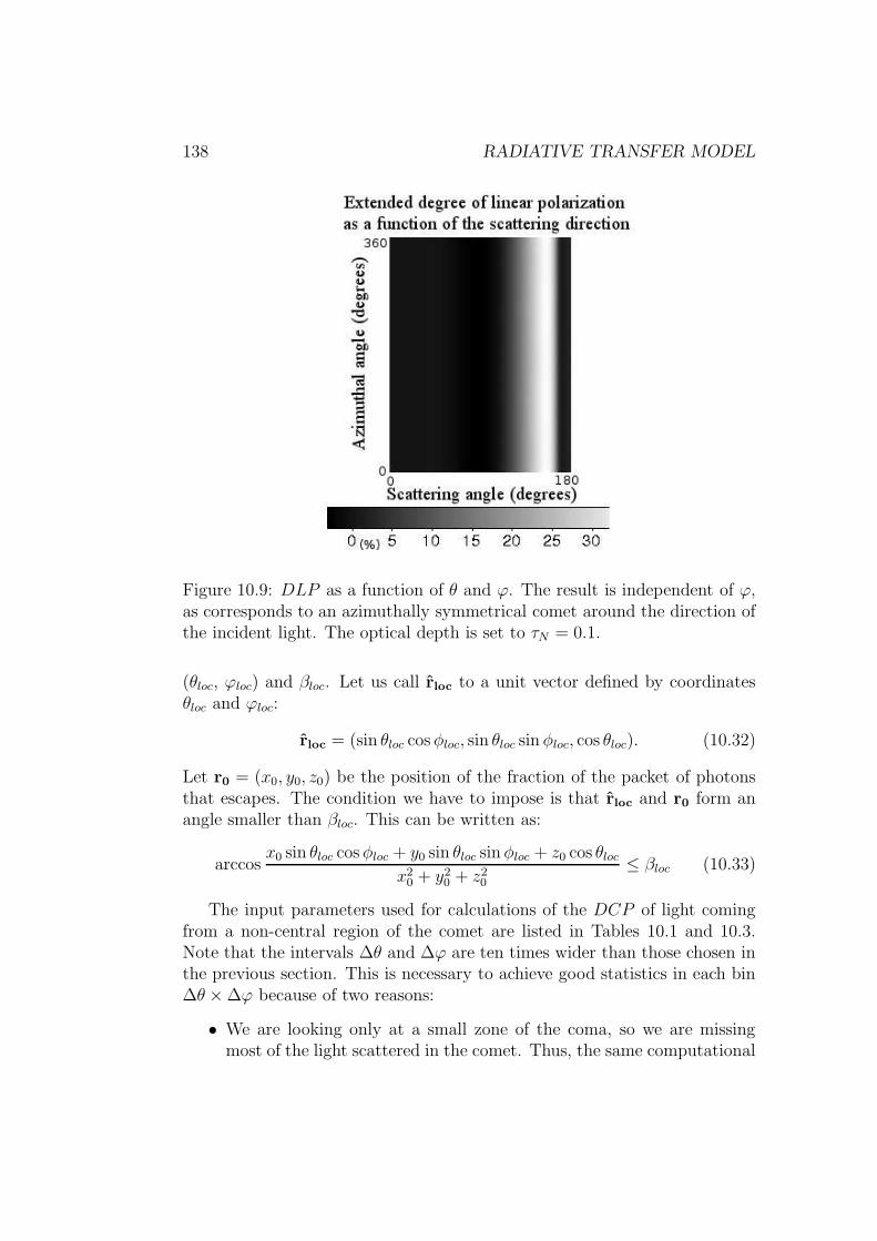
138 RADIATIVE TRANSFER MODEL
Figure 10.9: DLP as a function of θ and ϕ. The result is independent of ϕ,as corresponds to an azimuthally symmetrical comet around the direction ofthe incident light. The optical depth is set to τN = 0.1.
(θloc, ϕloc) and βloc. Let us call rloc to a unit vector defined by coordinatesθloc and ϕloc:
rloc = (sin θloc cos φloc, sin θloc sin φloc, cos θloc). (10.32)
Let r0 = (x0, y0, z0) be the position of the fraction of the packet of photonsthat escapes. The condition we have to impose is that rloc and r0 form anangle smaller than βloc. This can be written as:
arccosx0 sin θloc cos φloc + y0 sin θloc sin φloc + z0 cos θloc
x20 + y2
0 + z20
≤ βloc (10.33)
The input parameters used for calculations of the DCP of light comingfrom a non-central region of the comet are listed in Tables 10.1 and 10.3.Note that the intervals ∆θ and ∆ϕ are ten times wider than those chosen inthe previous section. This is necessary to achieve good statistics in each bin∆θ × ∆ϕ because of two reasons:
• We are looking only at a small zone of the coma, so we are missingmost of the light scattered in the comet. Thus, the same computational

LOCAL OBSERVATIONS 139
Figure 10.10: Comparison of the EDLP calculated with the Monte Carlomodel to the theoretical value in single scattering conditions, derived fromthe scattering matrix. The agreement is excellent.
NPHOT 108
NRING 108
τN 2.5∆θ 10
∆ϕ 10
θloc 60
ϕloc 0
βloc 10
Table 10.3: Specific input parameters used to calculate the DCP of lightcoming from a non-central local region of the comet (see Fig. 10.12).
effort to launch and track the evolution of the same number of packetsof photons as in the previous section is being performed, but a muchlower signal is being recorded at each bin.

140 RADIATIVE TRANSFER MODEL
Figure 10.11: A small conical region of the comet (plotted in red) is definedby angular coordinates (θloc, ϕloc) and an angle βloc. A unit vector r is definedby (θloc, ϕloc). Light that escapes from the comet is considered only if thevector position r0 of the fractions of the packets of photons that escape iscontained into the red cone.
• We are using a much larger optical thickness than in Sec. 10.4 (25 timeslarger), so much more absorption occurs in the coma, and the amountof outgoing radiation energy is much lower for the same number oflaunched packets of photons.
We checked the statistical stability by repeating the calculations with NPHOT =8 · 108, and verifying the convergence of the obtained results.
Fig. 10.12 presents the results of the calculations on the DCP (left panel)for rmax = 20 µm, along with an illustration of the meaning of the plot (rightpanel).
The big light blue circle of the right panel of Fig. 10.12 represents thecomet. It is illuminated from the back. Only light scattered from a 10 wideregion was considered. That zone is marked in the figure by a small darkblue circle. From that region, light is scattered in all directions. We justpresent results for −90 ≤ ϕ ≤ 90 because the best statistics was achievedfor those angles.
We find three main features in the results presented in Fig. 10.12:

LOCAL OBSERVATIONS 141
Figure 10.12: Results for the calculations of the DCP with our radiativetransfer model (left panel). All parameters of the model are taken fromTables 10.1 and 10.3, except for rmax, that is set to 20 µm. An illustrationof the meaning of the left plot is presented in the right panel. Only lightcoming from a small region (small dark blue circle) is recorded. Radiationis emitted in all directions from that zone. Only results for light scatteredat ϕ within [−90, 90] are presented, because the best statistics is achievedwithin this interval.
1. The upper part and the lower part of the left panel of Fig. 10.12 arecolor-complementary: the white bins of the upper part correspond tothe black bins of the lower part.
2. For angles close to the backscattering, higher values of the DCP (inabsolute value) are calculated than for forward-scattering angles.
3. The calculated values of the DCP are about one or two orders of mag-nitude below those of the observations.
Feature (1) can be understood in terms of symmetry: if a certain DCPappears by any means for positive values of the azimuthal angle, oppositevalues must be given when observing from a direction with ϕ < 0. The proofis again based in symmetry arguments, and it is identical to that given inSec. 5.2.

142 RADIATIVE TRANSFER MODEL
Regarding feature (2), we think that this may be an argument to supportthe idea that multiple scattering is the responsible for the observed DCP ,because light scattered in the back direction has generally undergone morescattering events that light passing by the comet with little interaction withthe grains of the coma. If multiple scattering along with asymmetry of theobservation scenario is the mechanism producing CP , it makes sense thatthe more important the multiple scattering becomes, the higher values of theDCP are reached.
About feature (3), we tried to achieve higher values of the DCP by mak-ing calculations for larger particles. Results presented in Fig. 10.12 corre-spond to particles with a maximum size of 20 µm. According to Sec. 2.4,much larger grains may be present in the coma of comets (up to the orderof 1 mm). We performed calculations of the DCP for two samples withrmax = 200 µm and rmax = 2 mm. The rest of the parameters of the codewere the same as for the result showed in Fig. 10.12.
The Mie scattering code implemented by Bohren & Huffman presentssome convergence problems when particles become as large as 2 mm. In orderto get accurate results, we used a large number of sizes to sample the sizedistribution (5000), and adjusted the accuracy parameters of the program.Both, the size distribution and the non-zero independent scattering matrixelements (see Sec. 3.6.2) are plotted in Figs. 10.13 and 10.14, respectively.All curves are smooth, and regarding the scattering matrix, conditions atexact forward- and backward-scattering are fulfilled (see, e.g., [30]). Thesearguments lead us to rely on the calculated size-averaged scattering matrix.
Fig. 10.15 shows the calculated DCP for the samples with rmax = 200 µm(left panel), and for the sample of rmax = 2 mm (right panel).
The calculated values are of the same order of those obtained for rmax =20 µm (Fig. 10.12). Hence, the local observation of a symmetrical cometwhose coma is formed by spherical grains, cannot explain the observed DCPin comets.
10.6 Asymmetry of the coma
The distribution of dust particles around the nucleus of a comet might beinhomogeneous. For instance, there might be active regions of the surface ofthe nucleus in some specific parts, or there might be more sublimation in theside of the comet that faces the Sun. This asymmetrical distribution couldlead to the asymmetry of the coma around the optical axis, so some DCPcould arise from this mechanism.
We divided the coma of the comet into two halves, the separation plane
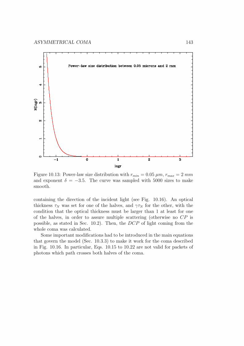
ASYMMETRICAL COMA 143
Figure 10.13: Power-law size distribution with rmin = 0.05 µm, rmax = 2 mmand exponent δ = −3.5. The curve was sampled with 5000 sizes to makesmooth.
containing the direction of the incident light (see Fig. 10.16). An opticalthickness τN was set for one of the halves, and γτN for the other, with thecondition that the optical thickness must be larger than 1 at least for oneof the halves, in order to assure multiple scattering (otherwise no CP ispossible, as stated in Sec. 10.2). Then, the DCP of light coming from thewhole coma was calculated.
Some important modifications had to be introduced in the main equationsthat govern the model (Sec. 10.3.3) to make it work for the coma describedin Fig. 10.16. In particular, Eqs. 10.15 to 10.22 are not valid for packets ofphotons which path crosses both halves of the coma.

144 RADIATIVE TRANSFER MODEL
Figure 10.14: Non-zero independent elements of the scattering matrix ofa sample of spheres with a size distribution as that given in Fig. 10.13.The curves are smooth, and all necessary conditions at the forward- andbackward-scattering directions are fulfilled.
Suppose that a packet of photons located at P0 (see Fig. 10.16) takesits next step to its destination Pd, where Pd might be the nucleus (A), theinfinity (B) or another point P2 in the coma (C). For each case, there existfour possibilities:
1. P0, Pd ∈ τN
2. P0, Pd ∈ γτN
3. P0 ∈ τN , Pd ∈ γτN
4. P0 ∈ γτN , Pd ∈ τN
Some simple algebraic manipulations leads to the following equations forthe cases enumerated above:

ASYMMETRICAL COMA 145
Figure 10.15: Results for the calculations of the DCP with our radiativetransfer model. All parameters of the model are taken from Tables 10.1 and10.3, except for rmax, that is set to 200 µm for the left panel. Only resultsfor light scattered at ϕ within [−90, 90] are presented, because the beststatistics is achieved within this interval.
A1)
τc =τNRN
∆
(
arctanr0 · e + sc
∆− arctan
r0 · e
∆
)
, (10.34)
if ∆ 6= 0, with ∆ =√
r20 − (r0 · e)2.
A2)The same as in A1 but exchanging τN by γτN .
A3)
τc =τNRN
∆
(
arctanr0 · e + s1
∆− arctan
r0 · e
∆
)
+
γτNRN
∆
(
arctanr1 · e + s2
∆− arctan
r1 · e
∆
)
, (10.35)
if ∆ 6= 0, with ∆ =√
r20 − (r0 · e)2 =
√
r21 − (r1 · e)2. Longitude s1 is the
distance from P0 to P1 (see Fig. 10.16), and s2 = sc − s1.

146 RADIATIVE TRANSFER MODEL
Figure 10.16: Asymmetrical coma formed by two halves of different opticalthicknesses: τN and γτN . The optical axis is contained in the plane thatseparates both parts. A packet of photons travels from a point (x0, y0, z0) inone part to (x2, y2, z2) in the other crossing the interface plane at (x1, y1, z1).
A4)
The same as in A3 but exchanging τN by γτN .
B1)
τ∞ =τNRN
∆
(
π
2− arctan
r0 · e
∆
)
, (10.36)
if ∆ 6= 0, with ∆ =√
r20 − (r0 · e)2.
B2)
The same as in B1 but exchanging τN by γτN .

ASYMMETRICAL COMA 147
B3)
τ∞ =τNRN
∆
(
arctanr0 · e + s1
∆− arctan
r0 · e
∆
)
+
γτNRN
∆
(
π
2− arctan
r1 · e
∆
)
, (10.37)
if ∆ 6= 0, with ∆ =√
r20 − (r0 · e)2 =
√
r21 − (r1 · e)2.
B4)The same as in B3 but exchanging τN by γτN .
C1) y0 ≥ 0, ey ≥ 0
s = ∆ tan∆τ
τNRN+ arctan
r0 · e
∆− r0 · e, (10.38)
if ∆ 6= 0, with ∆ =√
r20 − (r0 · e)2.
C2) y0 < 0, ey < 0The same as in C1 but exchanging τN by γτN .
C3) y0 ≥ 0, ey < 0
Let us suppose ∆ 6= 0, with ∆ =√
r20 − (r0 · e)2 =
√
r21 − (r1 · e)2.
Then, we define:
τsep =τNRN
∆
(
arctanr0 · e + sc
∆− arctan
r0 · e
∆
)
. (10.39)
If τ ≤ τsep (τ given by Eq. 10.8):
s = ∆ tan∆τ
τNRN
+ arctanr0 · e
∆− r0 · e. (10.40)
Otherwise:
s = ∆ tan∆τ
τNRN
+ arctanr0 · e
∆− r0 · e +
∆ tan∆τ
γτNRN
+ arctanr1 · e
∆− r1 · e (10.41)
C4) y0 < 0, ey ≥ 0

148 RADIATIVE TRANSFER MODEL
Identical as in C3 but exchanging τN by γτN .
The special case ∆ = 0 for cases A1, A2, B1, B2, C1 and C2 are presentedbelow. For any other case ∆ cannot be equal to zero because a packetof photons cannot cross from one half of the coma to the other in radialdirection.
A1) For packets of photons approaching the nucleus, Eq. 10.18, and forthose travelling far away, Eq. 10.19 (substituting in both cases τ by τc ands by sc).
A2) The same as in A1 but substituting τN by γτN .
B1) Eq. 10.20.
B2) The same as in B2 but substituting τN by γτN .
C1) For packets of photons approaching the nucleus, Eq. 10.18, and forthose travelling far away, Eq. 10.19.
C2) The same as in C1 but changing τN by γτN .
NPHOT 108
NRING 108
τN 0.5γ 10∆θ 1
∆ϕ 1
Table 10.4: Specific input parameters of the model that were used to calculatethe DCP of light scattered by an azimuthally asymmetrical comet aroundthe optical axis (see Fig. 10.16).
Fig. 10.17 shows the DCP produced by an asymmetrical comet withparameters given in Tables 10.1 and 10.4. Results for two different values ofrmax are shown: 200 µm on the left and 2 mm on the right panel. Despitethe artificial asymmetry that we imposed to the comet, no significant DCPcompared to the observations was achieved by this mechanism either.

LOCAL OBSERVATION OF AN ASYMMETRICAL COMA 149
Figure 10.17: Results for the calculations of the DCP with our radiativetransfer model. All parameters of the model are taken from Tables 10.1 and10.4, except for rmax, that was set to 200 µm for the left panel, and 2 mmfor the right one. Light coming from the whole comet is taken into account.
10.7 Local observation of an asymmetrical coma
Although mechanisms presented in Secs. 10.5 and 10.6 did not produce bythemselves values of the DCP comparable to the observations, a mixture ofboth of them may give a different result. In the present section we calculatethe DCP given by the same system as presented in Sec. 10.6. Moreover,the comet is locally observed as in the case presented in Sec. 10.5. Theobservation region is located in the half of the coma with the highest opticalthickness (see Fig. 10.18). In this way, the maximum multiple scatteringconditions are assured.
Specific input parameters for this run of the model are given in Table10.5, and results are presented in Fig. 10.19.
Slightly higher values of the DCP have been achieved than in Secs. 10.5and 10.6, but still the calculated values are one or two orders of magnitude

150 RADIATIVE TRANSFER MODEL
Figure 10.18: Target system to study in the present section: a comet isdivided into two parts of different optical thicknesses, with multiple scatteringat least in one of them. It is observed locally, i.e., just light coming from acertain small region of the coma is recorded. This region is located in thehalf of the coma with the highest optical thickness.
below the observations. However, we still rely on multiple scattering asthe responsible mechanism of the observed DCP in comets because of thefollowing reasons:
• As pointed out in Sec. 4.3, two common features to several observa-tions of the DCP in comets are the tendency to the DCP to vanishwhen approaching the nucleus and when increasing the aperture of theused diaphragm. Local observation in a multiple scattering scenariois an explanation for both of these features, but the other discussedmechanisms can hardly be compatible with these facts.
• All mechanisms based on multiple scattering that we have studied inthe present chapter, systematically give a non-negligible DCP , just oneor two orders of magnitude below the observations.

LOCAL OBSERVATION OF AN ASYMMETRICAL COMA 151
NPHOT 107
NRING 107
rmax 200 µmτN 0.5γ 10∆θ 10
∆ϕ 10
θloc 60
ϕloc 270
βloc 10
Table 10.5: Specific input parameters used to calculate the DCP of lightcoming from a non-central local region of an azimuthally asymmetrical cometaround the optical axis (see Fig. 10.18).
Figure 10.19: Calculations of the DCP with our radiative transfer model fora locally observed asymmetrical comet around the direction of the incidentlight (see Fig. 10.18). All parameters of the model are taken from Tables10.1 and 10.5.
• Our calculations only deal with spherical particles, and grains with

152 RADIATIVE TRANSFER MODEL
more realistic shapes may yield higher values of the DCP .
• We are considering only silicates, but not carbon-like refractive indices.Changing the refractive index in the calculations may lead to values ofthe DCP comparable to the observations.
Using non-spherical (even asymmetrical) particles may yield highest val-ues of the DCP . To make a good approximation to a real comet, we need tocalculate the scattering matrices of non-spherical particles with sizes rangingfrom the order of 0.1 µm to 1 mm approximately (see Sec. 2.4). Techniquesdescribed in Sec. 3.5 are adequate to obtain the scattering matrices of par-ticles of the order of the wavelength, and ray-tracing models [56] can makeaccurate calculations for particles much larger than the wavelength. For ir-regular shapes, there is still a wide range of sizes whose scattering propertiescannot be calculated by any known method.
10.8 Conclusions
• A new model of radiative transfer in the coma of comets has beendeveloped, including any kind of particles either in conditions of singleor multiple scattering.
• A certain DCP appears in an azimuthally symmetrical comet if webreak the symmetry of the system by considering only light comingfrom a non-central zone of the comet in conditions of multiple scatter-ing. However, the obtained values of the DCP are one or two ordersof magnitude below the observations when using spherical silicate-likeparticles for the dust grains of the coma.
• A non-negligible DCP arises when integrating all light coming froma non-symmetrical comet (coma divided into two part with very dif-ferent optical thicknesses, the optical axis contained in the plane thatseparates both parts). Again the values are one or two orders of mag-nitude below the observations. Observing just a small region of thehigh-density half of the coma does not lead to results comparable tothe observations either.
• Using non-spherical particles or a carbon-like refractive index for thegrains of the coma may yield higher calculated values of the DCP .

Chapter 11
Conclusions
Regarding the observations:
• In all cases, the observed DCP for a certain region of the comet ishighly variable in time (day-to-day and even minute-to-minute varia-tions).
• The DCP approaches zero when the aperture of the diaphragm in-creases in observations of Halley.
• For accurate observations, such as those of Hale-Bopp, and others ac-quired later, the DCP approaches zero when looking at the nuclearregion of the comet.
• In most cases, both positive and negative values of the DCP are ob-tained, except for two exceptions: observations of Hale-Bopp by Rosen-bush et al. [63], where all obtained values were negative, and observa-tions of Comet C/1999 S4. For the latter case, all observed values werepositive for the smallest phase angle (60.9). Then both positive andnegative values appeared at intermediate values of φ, becoming finallymostly negative at φ ≈ 120.
Regarding the candidate mechanisms to produce CP :
• The breaking of the symmetry of a comet around the direction of theincident light is a necessary condition for a mechanism to circularlypolarize the scattered light.
• A complete list of candidates to produce CP of light scattered in cometsis the following:
153

154 CONCLUSIONS
1. Alignment of non-spherical grains.
2. Breaking of the mirror symmetry.
3. Optical activity of the material composing the particles.
4. Local observation of a non-central region.
5. Inhomogeneous distribution of particles in the coma.
6. Asymmetrical nucleus of the comet.
Regarding the alignment of non-spherical particles:
• Prolate rectangular prisms of dimensions 0.1 µm×0.1 µm×0.2 µm witha density of 3 gcm−3 are aligned in 1.8 · 104 s due to the bombardmentby the solar wind particles at an heliocentric distance of 1AU .
• The alignment occurs with the longest axis of the particle orientedperpendicularly to the direction of the incident light.
• Oblate particles with the same volume and density as the prolate ones,but with axes ratios 2:2:1, are not aligned even in 2.4 · 105 s.
• If particles in comets were actually aligned and the responsible mech-anism for the alignment was the bombardment by the solar wind, wewould not obtained any non-zero DCP , because the cloud of alignedparticles would be symmetrical around the direction of the incidentlight.
Regarding asymmetrical model particles:
• For the snake-like shape with seven monomers and m = 1.5 + i0.001,the mean amplitude of the curve of the DCP is close to zero for smallsize parameters (as corresponds to the Rayleigh domain), and thengrows as the size parameters of the monomers increases to x = 1.8, inwhich case a maximum larger than 2% is found. When the size param-eter becomes larger than x = 1.8, the amplitude decreases gradually,becoming essentially zero for x = 10.
• For the snake-like shape with seven monomers and m = 1.5+i0.001, thecomplexity of the curves of the DCP increases always when increasingthe size of the particle.
• Single scattering of optically inactive asymmetrical particles in randomorientations can give large values of the DCP of the scattered light(more than 2%), at least for a snake-like aggregate composed of sevenspherical monomers with m = 1.5 + i0.001.

CONCLUSIONS 155
• If we use a typical power-law size distribution, the curves of the DCPcorresponding to snake-like aggregates made of 7 monomers with m =1.5+i0.001 still show values of the DCP of the order of the observations(≈ 0.1% or less).
• Increasing the absorption of the particles makes the main amplitude ofthe curves of the DCP to decrease, at least for snake-like aggregatesof seven monomers with x = 2 and Re(m) = 1.5. However, the effectis the opposite if the imaginary part of the refractive index is fixed toIm(m) = 0.001 and the real part is increased.
• By increasing the number of monomers of an aggregate, but keeping thewhole size constant, the number of maxima and minima of DCP curvesincreases and the amplitudes of these decreases, at least for snake-likeparticles with x = 2 and m = 1.5 + i0.001.
• It is not necessary that monomers composing the aggregates are equal-sized to obtain high values of the DCP . In fact, the snake particlegives almost identical curves of the DCP even taking for the monomersvolumes as different as V0, V0 + 30%V0 and V0 − 30%V0.
• If the snake particle made of 7 monomers is compared to the MrSanchez particle (made of 25 monomers and more complex), the meanamplitude of the curve of the DCP is larger for the snake at small sizeparameters (X . 4), but it is comparable for both shapes if the size ofthe aggregates is large enough (X & 7).
• The peaks of the curves of the DCP may be due to resonances. Thereexist two types of peaks: primary peaks (fixed number, at fixed scat-tering angles and due to resonances by the substructures that producethe asymmetry of the particle), and secondary peaks (the number in-creases with the size of the grain, not at fixed scattering angles and dueto resonances by the monomers).
Regarding irregular particles:
• Primary peaks have smaller amplitudes in randomly built aggregatesthan in the asymmetrical model particles used in the previous chapter.
• Secondary peaks have larger amplitudes than primary ones in randomlybuilt aggregates.

156 CONCLUSIONS
• The DCP of a sample of particles averaged over sizes for a fixed shapeis mainly determined by the primary peaks, as in the case of modelparticles.
• A lower DCP arises from a size-averaged sample of randomly builtaggregates of a fixed shape than for that of model grains.
• The DCP rapidly tends to zero when building a sample with just afew size-averaged shapes.
• Single scattering by asymmetrical particles in random orientation doesnot make a significant contribution of the observed DCP in comets.
Regarding optical activity:Althoug there are evidences that optical active materials are present in
comets, we rule out the scattering by optically active grains as the responsiblemechanism for the DCP observed in comets, because it does not match someof the features found in the observations.
Regarding multiple scattering:
• A new model of radiative transfer in the coma of comets has beendeveloped, including any kind of particles either in conditions of singleor multiple scattering.
• A certain DCP appears in an azimuthally symmetrical comet if webreak the symmetry of the system by considering only light comingfrom a non-central zone of the comet in conditions of multiple scatter-ing. However, the obtained values of the DCP are one or two ordersof magnitude below the observations when using spherical silicate-likeparticles for the dust grains of the coma.
• A non-negligible DCP arises when integrating all light coming froma non-symmetrical comet (coma divided into two part with very dif-ferent optical thicknesses, the optical axis contained in the plane thatseparates both parts). Again the values are one or two orders of mag-nitude below the observations. Observing just a small region of thehigh-density half of the coma does not lead to results comparable tothe observations either.
• Using non-spherical particles or a carbon-like refractive index for the-grains of the coma may yield higher calculated values of the DCP .

Chapter 12
Future work
• To perform calculations of the DCP with the Monte Carlo radiativetransfer model by using non-spherical particles of sizes ranging from0.1 µm to 1 mm.
• To perform calculations of the DCP with the Monte Carlo radiativetransfer model by using a refractive index typical for amorphous carbon.
• To include the possibility to use a particular scattering matrix for eachparticle at each orientation in the Monte Carlo model, instead of usingaverage matrices.
• To include the possibility of a layered number density distribution ofparticles in the coma for the radiative transfer model in order to fit lin-ear polarization in situ measurements of the EDLP in the atmosphereof Titan (collaboration with Robert West-JPL).
• To include the possibility of dealing with numerical, instead of ana-lytical, number density distributions of particles in the coma for theradiative transfer model. This would be applicable, e.g., to the outputsof the circumnuclear coma hydrodynamic models by Crifo [10].
• To build a numerical code to calculate the DCP given by opticallyactive particles.
• To mix together several candidate mechanisms producing CP by using,in the radiative transfer model, scattering matrices corresponding toaligned, asymmetrical and optically active particles.
• To build an adequate model of scattering on surfaces and use it tosimulate the reflection of light on the nucleus of the comet.
157


Appendix A
General method to samplevalues of a variable from itsprobability density function
The probability density p of a variable x is defined such as the probabilityof x to be between x1 and x2 is given by P (x1 ≤ x ≤ x2) =
∫ x2
x1
p(x)dx. Theprobability is equal to the area under the curve of p(x) from x1 to x2: equalareas means equal probabilities. Let us divide now the area under the curveof p(x) into infinite regions of elemental surface dS. The probability of x tobe within each of those regions is the same, because they all have the samearea. A way of sampling x is to uniformly randomly choose one region of areadS (a), and then calculate the coordinate x corresponding to that region (b).Step (a) can be achieved as follows: the chosen region is the last elementalsurface added to the integral S(x) =
∫ x
0p(x′)dx′ to make it a certain value ξ.
If ξ is uniformly distributed, all regions of area dS will be equally probable.Step (b) simply consists on finding the value of x that makes S(x) = ξ.
In summary, a way to sample values of x from a probability densityfunction p is the following:
1. To determine a uniform random number ξ within [0, 1].
2. To work x out from S(x) = ξ.
159


Bibliography
[1] C.F. Bohren. Light scattering by an optically active sphere. ChemicalPhysics Letters, 29:458–462, 1974.
[2] C.F. Bohren. Scattering of electromagnetic waves by an optically activecylinder. J. Colloid Interface Sci., 66:105–109, 1978.
[3] C.F. Bohren and D.R. Huffman. Absorption and Scattering of Light bySmall Particles. Wiley, 1983.
[4] M. Born, E. Wolf, and A.B. Bhatia. Principles of Optics. CambridgeUniversity Press, October 1999.
[5] D. Brownlee, P. Tsou, J. Aleon, C.M.O’D. Alexander, T. Araki, S. Bajt,G.A. Baratta, R. Bastien, P. Bland, P. Bleuet, J. Borg, J.P. Bradley,A. Brearley, F. Brenker, S. Brennan, J.C. Bridges, N.D. Browning, J.R.Brucato, E. Bullock, M.J. Burchell, H. Busemann, A. Butterworth,M. Chaussidon, A. Cheuvront, Miaofang Chi, Mark J. Cintala, B. C.Clark, S.J. Clemett, G. Cody, L. Colangeli, G. Cooper, P. Cordier,C. Daghlian, Z. Dai, L. D’Hendecourt, Z. Djouadi, G. Dominguez,T. Duxbury, J.P. Dworkin, D.S. Ebel, T.E. Economou, S. Fakra, S.A.J.Fairey, S. Fallon, G. Ferrini, T. Ferroir, H. Fleckenstein, C. Floss,G. Flynn, I.A. Franchi, M. Fries, Z. Gainsforth, J.-P. Gallien, M. Genge,M.K. Gilles, P. Gillet, J. Gilmour, D.P. Glavin, M. Gounelle, M.M.Grady, G.A. Graham, P.G. Grant, S.F. Green, F. Grossemy, L. Gross-man, J.N. Grossman, Y. Guan, K. Hagiya, R. Harvey, P. Heck, G.F. Her-zog, P. Hoppe, F. Horz, J. Huth, I.D. Hutcheon, K. Ignatyev, H. Ishii,M. Ito, D. Jacob, C. Jacobsen, S. Jacobsen, S. Jones, D. Joswiak,A. Jurewicz, A.T. Kearsley, L.P. Keller, H. Khodja, A.L.D. Kilcoyne,J. Kissel, A. Krot, F. Langenhorst, A. Lanzirotti, L. Le, L.A. Leshin,J. Leitner, L. Lemelle, H. Leroux, M.-C. Liu, K. Luening, I. Lyon,G. MacPherson, M.A. Marcus, K. Marhas, B. Marty, G. Matrajt,K. McKeegan, A. Meibom, V. Mennella, K. Messenger, S. Messenger,T. Mikouchi, S. Mostefaoui, T. Nakamura, T. Nakano, M. Newville,
161
162 BIBLIOGRAPHY
L.R. Nittler, I. Ohnishi, K. Ohsumi, K. Okudaira, D.A. Papanastas-siou, R. Palma, M.E. Palumbo, R.O. Pepin, D. Perkins, M. Perronnet,P. Pianetta, W. Rao, F.J.M. Rietmeijer, F. Robert, D. Rost, A. Ro-tundi, R. Ryan, S.A. Sandford, C.S. Schwandt, T.H. See, D. Schlutter,J. Sheffield-Parker, A. Simionovici, S. Simon, I. Sitnitsky, C.J. Snead,M.K. Spencer, F. J. Stadermann, A. Steele, T. Stephan, R. Stroud,J. Susini, S.R. Sutton, Y. Suzuki, M. Taheri, S. Taylor, N. Tes-lich, K. Tomeoka, N. Tomioka, A. Toppani, J.M. Trigo-Rodrıguez,D. Troadec, A. Tsuchiyama, A.J. Tuzzolino, T. Tyliszczak, K. Ue-sugi, M. Velbel, J. Vellenga, E. Vicenzi, L. Vincze, J. Warren, I. We-ber, M. Weisberg, A.J. Westphal, S. Wirick, D. Wooden, B. Wopenka,P. Wozniakiewicz, I. Wright, H. Yabuta, H. Yano, E.D. Young, R.N.Zare, T. Zega, K. Ziegler, L. Zimmerman, E. Zinner, and M. Zolensky.Comet 81P/Wild 2 under a microscope. Science, 314:1711, 2006.
[6] S. Chandrasekhar. Radiative Transfer. Courier Dover Publications,1960.
[7] R.W. Christy, J.R. Reitz, and F.J. Milford. Fundamentos de la TeorıaElectromagnetica. Addison-Wesley Iberoamericana S. A., 1996.
[8] S.R. Cloude. Group theory and polarization algebra. Optik, 75:26, 1986.
[9] J.F. Crifo, M. Fulle, N.I. Komle, and K. Szego. Nucleus-coma structuralrelationships: lessons from physical models. In Comets II, pages 471–503. University of Arizona Press, 2004.
[10] J.F. Crifo, G.A. Lukianov, A.V. Rodionov, G.O. Khanlarov, and V.V.Zakharov. Comparison between Navier-Stokes and direct Monte-Carlosimulations of the circumnuclear coma. I - Homogeneous, sphericalsource. Icarus, 156:249–268, 2002.
[11] P. Debye. Der lichtdruck auf kugeln von beliebigem material. Annalender Physik, 335:57–136, 1909.
[12] J.C. del Toro Iniesta. Introduction to Spectropolarimetry. CambridgeUniversity Press, 2003.
[13] A.Z. Dolginov and I.G. Mitrofanov. Orientation of cometary dust andpolarization observations of comets. Soviet Astronomy, 19:758–764,1976.

BIBLIOGRAPHY 163
[14] A. Dollfus and J.-L. Suchail. Polarimetry of grains in the coma ofP/Halley. I - Observations. Astronomy and Astrophysics, 187:669–688,November 1987.
[15] M. Donahue, J. Bennett, N. Schneider, and M. Voit. The EssentialCosmic Perspective. Addison-Wesley, 2006.
[16] B.T. Draine and P.J. Flatau. Discrete-dipole approximation for scatter-ing calculations. Journal of the Optical Society of America A, 11:1491–1499, 1994.
[17] B.T. Draine and P.J. Flatau. User guide for the discrete dipole approx-imation code DDSCAT 7.0. http://arXiv.org/abs/0809.0337v5, 2008.
[18] A. Einstein. Uber einen die erzeugung und verwandlung des lichtesbetreffenden heuristischen gesichtspunkt. Annalen der Physik, 322:132–148, 1905.
[19] M.C. Festou, H. Rickman, and R.M. West. Comets. I - Concepts andobservations. Astronomy and Astrophysics Review, 4:363–447, 1993.
[20] M. Fulle. Motion of cometary dust. In Comets II, pages 565–575. Uni-versity of Arizona Press, 2004.
[21] D.P. Glavin, J.P. Dworkin, and S.A. Sandford. Detection of cometaryamines in samples returned by Stardust. Meteoritics and Planetary Sci-ence, 43:399–413, 2008.
[22] D. Guirado, J.W. Hovenier, and F. Moreno. Circular polarization oflight scattered by asymmetrical particles. Journal of Quantitative Spec-troscopy and Radiative Transfer, 106:63–73, 2007.
[23] D. Guirado, F. Moreno, and J.W. Hovenier. Circular polarization oflight scattered by randomly built aggregates. In X Conference on Elec-tromagnetic & Light Scattering by Non-Spherical Particles, pages 45–48,Bodrum (Turkey), 2007.
[24] D. Guirado, F. Moreno, and M.I. Mishchenko. A new mechanism pos-sibly explaining the circular polarization of light scattered in comets:asymmetry of the comet itself. In XI Conference on Electromagnetic &Light Scattering by Non-Spherical Particles, Hertfordshire (UK), 2008.
[25] J.E. Hansen and L.D. Travis. Light scattering in planetary atmospheres.Space Science Reviews, 16:527–610, October 1974.

164 BIBLIOGRAPHY
[26] F. Horz, R. Bastien, J. Borg, J.P. Bradley, J.C. Bridges, D.E. Brown-lee, M.J. Burchell, M. Chi, M.J. Cintala, Z.R. Dai, Z. Djouadi,G. Domınguez, T.E. Economou, S.A.J. Fairey, C. Floss, I.A. Franchi,G.A. Graham, S.F. Green, P. Heck, P. Hoppe, J. Huth, H. Ishii, A.T.Kearsley, J. Kissel, J. Leitner, H. Leroux, K. Marhas, K. Messenger, C.S.Schwandt, T.H. See, C. Snead, F.J. Stadermann, T. Stephan, R. Stroud,N. Teslich, J.M. Trigo-Rodrıguez, A.J. Tuzzolino, D. Troadec, P. Tsou,J. Warren, A. Westphal, P. Wozniakiewicz, I. Wright, and E. Zinner.Impact features on Stardust: implications for comet 81P/Wild 2 dust.Science, 314:1716, 2006.
[27] J.W. Hovenier. Measuring scattering matrices of small particles at opti-cal wavelengths. In Light Scattering by Nonspherical Particles: Theory,Measurments and Applications., page 355. Academic Press, 2000.
[28] J.W. Hovenier, C. van der Mee, and H. Domke. Transfer of PolarizedLight in Planetary Atmospheres. Springer, 2004.
[29] J.W. Hovenier and C.V.M. van der Mee. Testing scattering matrices:a compendium of recipes. Journal of Quantitative Spectroscopy andRadiative Transfer, 55:649–661, 1996.
[30] J.W. Hovenier and C.V.M. van der Mee. Basic relationships for ma-trices describing scattering by small particles. In Light Scattering byNonspherical Particles: Theory, Measurements and Applications, pages61–85. Academic Press, 2000.
[31] K. Jockers. Observations of scattered light from cometary dust and theirinterpretation. Earth Moon and Planets, 79:221–245, 1997.
[32] H.U. Keller. Properties of cometary nuclei. In Revista Mexicana deAstronomıa y Astrofısica Conference Series, volume 35, page 285, IslaMargarita (Venezuela), 2009.
[33] H.U. Keller, C. Arpigny, C. Barbieri, R.M. Bonnet, S. Cazes, M. Cora-dini, C.B. Cosmovici, W.A. Delamere, W.F. Huebner, D.W. Hughes,C. Jamar, D. Malaise, H.J. Reitsema, H.U. Schmidt, W.K.H. Schmidt,P. Seige, F.L. Whipple, and K. Wilhelm. First Halley multicolour cam-era imaging results from Giotto. Nature, 321:320–326, 1986.
[34] M.S. Kelley and D.H. Wooden. The composition of dust in jupiter-family comets inferred from infrared spectroscopy. Planetary and SpaceScience, 57:1133–1145, 2009.

BIBLIOGRAPHY 165
[35] R.E. Kleinman and T.B.A. Senior. Rayleigh scattering. In Low andHigh Frequency Asymptotics. North-Holland: Sole distributors for theUSA and Canada, Elsevier Science Pub. Co, 1986.
[36] L. Kolokolova and K. Jockers. Composition of cometary dust from po-larization spectra. Planetary and Space Science, 45:1543–1550, 1997.
[37] L. Kolokolova, H. Kimura, K. Ziegler, and I. Mann. Light-scatteringproperties of random-oriented aggregates: Do they represent the proper-ties of an ensemble of aggregates? Journal of Quantitative Spectroscopyand Radiative Transfer, 100:199–206, 2006.
[38] A. Lazarian. Magnetic fields via polarimetry: progress of grain align-ment theory. Journal of Quantitative Spectroscopy and Radiative Trans-fer, 79:881–902, 2003.
[39] L. Lorenz. Uber die refractionconstante. Ann. Phys. Chem., 11:70–103,1880.
[40] A.E.H. Love. The scattering of electric waves by a dielectric sphere.In London. Math. Soc. Conference, volume 30, pages 308–321, London,1899.
[41] R.W. Maas, E.P. Ney, and N.J. Woolf. The 10-MICRON emission peakof comet Bennett 1969i. Astrophysical Journal, 160:L101, 1970.
[42] D.W. Mackowski and M.I. Mishchenko. Calculation of the T-matrix andthe scattering matrix for ensembles of spheres. Journal of the OpticalSociety of America A, 13:2266–2278, 1996.
[43] N. Manset and P. Bastien. Polarimetric observations of comets C/1995O1 Hale-Bopp and C/1996 B2 Hyakutake. Icarus, 145:203–219, May2000.
[44] E.P. Mazets, R.L. Aptekar, S.V. Golenetskii, Y.A. Guryan, A.V.Dyachkov, V.N. Ilyinskii, V.N. Panov, G.G. Petrov, A.V. Savvin,R.Z. Sagdeev, I.A. Sokolov, N.G. Khavenson, V.D. Shapiro, and V.I.Shevchenko. Comet Halley dust environment from SP-2 detector mea-surements. Nature, 321:276–278, 1986.
[45] L.M. Merino-Gonzalez and E. Santos-Alaez. Algebra lineal. Publicatedby the authors, 1997.
[46] K. Metz and R. Haefner. Circular polarization near the nucleus of cometP/Halley. Astronomy and Astrophysics, 187:539–542, 1987.

166 BIBLIOGRAPHY
[47] G. Mie. Beitrage zur optik truber medien, speziell kolloidaler met-allosungen. Annalen der Physik, 330:377–445, 1908.
[48] M. Min, J.W. Hovenier, A. de Koter, L.B.F.M. Waters, and C. Dominik.The composition and size distribution of the dust in the coma of cometHale Bopp. Icarus, 179:158–173, 2005.
[49] M.I. Mishchenko and L.D. Travis. Satellite retrieval of aerosol propertiesover the ocean using polarization as well as intensity of reflected sunlight.Journal of Geophysical Research, 102(D14):16989–17013, 1997.
[50] M.I. Mishchenko, L.D. Travis, and A.A. Lacis. Multiple Scattering ofLight by Particles. Cambridge University Press, 2006.
[51] M.I. Mishchenko, L.D. Travis, and D.W. Mackowski. T-matrix compu-tations of light scattering by nonspherical particles: a review. Journalof Quantitative Spectroscopy and Radiative Transfer, 55:535–575, 1996.
[52] F. Moreno, O. Munoz, D. Guirado, and R. Vilaplana. Comet dust asa size distribution of irregularly shaped, compact particles. Journal ofQuantitative Spectroscopy and Radiative Transfer, 106:348–359, 2007.
[53] F. Moreno, O. Munoz, J.J. Lopez-Moreno, A. Molina, and J.L. Ortiz. AMonte Carlo code to compute energy fluxes in cometary nuclei. Icarus,156:474–484, 2002.
[54] A.V. Morozhenko, N.N. Kiselev, and A.L. Gural’Chuk. On the circularpolarization of comet Halley head. Kinematika i Fizika Nebesnykh Tel,3:89, April 1987.
[55] O. Munoz, F. Moreno, D. Guirado, J.L. Ramos, A. Lopez, F. Girela,J.M. Jeronimo, L.P. Costillo, and I. Bustamante. Experimental deter-mination of scattering matrices of dust particles at visible wavelengths:the IAA light scattering apparatus. Journal of Quantitative Spectroscopyand Radiative Transfer, 111:187–196, 2010.
[56] K. Muinonen, T. Nousiainen, P. Fast, K. Lumme, and J. Peltoneimi.Light scattering by Gaussian random particles: ray optics approxi-mation. Journal of Quantitative Spectroscopy and Radiative Transfer,55:577–601, 1996.
[57] P. Murdin. Encyclopedia of Astronomy and Astrophysics. Nature Pub-lishing Group, 2001.

BIBLIOGRAPHY 167
[58] T. Oguchi. Scattering properties of oblate raindrops & cross polarizationof radio waves due to rain. calculations at 19.3 & 34.8 GHz. J RadioRes. Lab. Jpn., 20:79–118, 1973.
[59] T. Oguchi. Light scattering by a spheroidal particle. Appl. Optics,14:29–49, 1975.
[60] A. Penttila, E. Zubko, K. Lumme, K. Muinonen, M.A. Yurkin,B. Draine, J. Rahola, A.G. Hoekstra, and Y. Shkuratov. Comparisonbetween discrete dipole implementations and exact techniques. Journalof Quantitative Spectroscopy and Radiative Transfer, 106:417–436, 2007.
[61] V. Rosenbush, N. Kiselev, N. Shakhovskoy, S. Kolesnikov, and V. Breus.Circular and linear polarization of comet C/2001 Q4 (NEAT). Why cir-cular polarization in comets is predominantly left-handed? In X Confer-ence on Electromagnetic & Light Scattering by Non-Spherical Particles,pages 181–184, Bodrum (Turkey), 2007.
[62] V. Rosenbush, L. Kolokolova, A. Lazarian, N. Shakhovskoy, and N. Kise-lev. Circular polarization in comets: observations of comet C/1999 S4(LINEAR) and tentative interpretation. Icarus, 186:317–330, 2007.
[63] V.K. Rosenbush, N.M. Shakhovskoj, and A.E. Rosenbush. Polarimetryof comet Hale-Bopp: linear and circular polarization, stellar occultation.Earth Moon and Planets, 78:381–386, 1999.
[64] H. Salo. Monte Carlo modeling of the net effects of coma scattering andthermal reradiation on the energy input to cometary nucleus. Icarus,76:253–269, 1988.
[65] S.A. Sandford, J. Aleon, C.M.O’D. Alexander, T. Araki, S. Bajt,G.A. Baratta, J. Borg, J.P. Bradley, D.E. Brownlee, J.R. Brucato,M.J. Burchell, H. Busemann, A. Butterworth, S.J. Clemett, G. Cody,L. Colangeli, G. Cooper, L. D’Hendecourt, Z. Djouadi, J.P. Dworkin,G. Ferrini, H. Fleckenstein, G.J. Flynn, I.A. Franchi, M. Fries, M.K.Gilles, D.P. Glavin, M. Gounelle, F. Grossemy, C. Jacobsen, L.P.Keller, A.L.D. Kilcoyne, J. Leitner, G. Matrajt, A. Meibom, V. Men-nella, S. Mostefaoui, L.R. Nittler, M.E. Palumbo, D.A. Papanastassiou,F. Robert, A. Rotundi, C.J. Snead, M.K. Spencer, F.J. Stadermann,A. Steele, T. Stephan, P. Tsou, T. Tyliszczak, A.J. Westphal, S. Wirick,B. Wopenka, H. Yabuta, R.N. Zare, and M.E. Zolensky. Organics cap-tured from comet 81P/Wild 2 by the Stardust spacecraft. Science,314:1720, 2006.

168 BIBLIOGRAPHY
[66] S.A. Stern. The evolution of comets in the Oort cloud and Kuiper belt.Nature, 424:639–642, 2003.
[67] W. Sun, Q. Fu, and Z. Chen. Finite-Difference Time-Domain solutionof light scattering by dielectric particles with a perfectly matched layerabsorbing boundary condition. Applied Optics, 38:3141–3151, 1999.
[68] H.C. van de Hulst. Light Scattering by Small Particles. Courier DoverPublications, 1981.
[69] R. Vilaplana, J. Canto, F. Moreno, and D. Guirado. The influence ofparticles shapes and sizes in the CO ice stretching mode. Earth, Planetsand Space, accepted for publication, 2009.
[70] J.R. Wait. Scattering of a plane wave from a circular dielectric cylinderat oblique incidence. Canadian Journal of Physics, 33:189–195, 1955.
[71] Y.-L. Xu and B.S. Gustafson. A generalized multiparticle Mie-solution:further experimental verification. Journal of Quantitative Spectroscopyand Radiative Transfer, 70:395–419, 2001.
[72] M.A. Yurkin and A.G. Hoekstra. User manual for the dis-crete dipole approximation code Amsterdam DDA (version 0.79).http://www.science.uva.nl/research/scs/Software/adda/index.html,2009.


![Me tomó unos minutos acostumbrarme a lo que ocurría: todos hablando al mismo tiempo. “[11:05] You have been added to the group. [11:09] Sradesmith:](https://img.pdfslide.us/doc/110x75/5528bde4497959977d8fb5b7/me-tomo-unos-minutos-acostumbrarme-a-lo-que-ocurria-todos-hablando-al-mismo-tiempo-1105-you-have-been-added-to-the-group-1109-sradesmith.jpg)