A screen for morphological complexity identifies

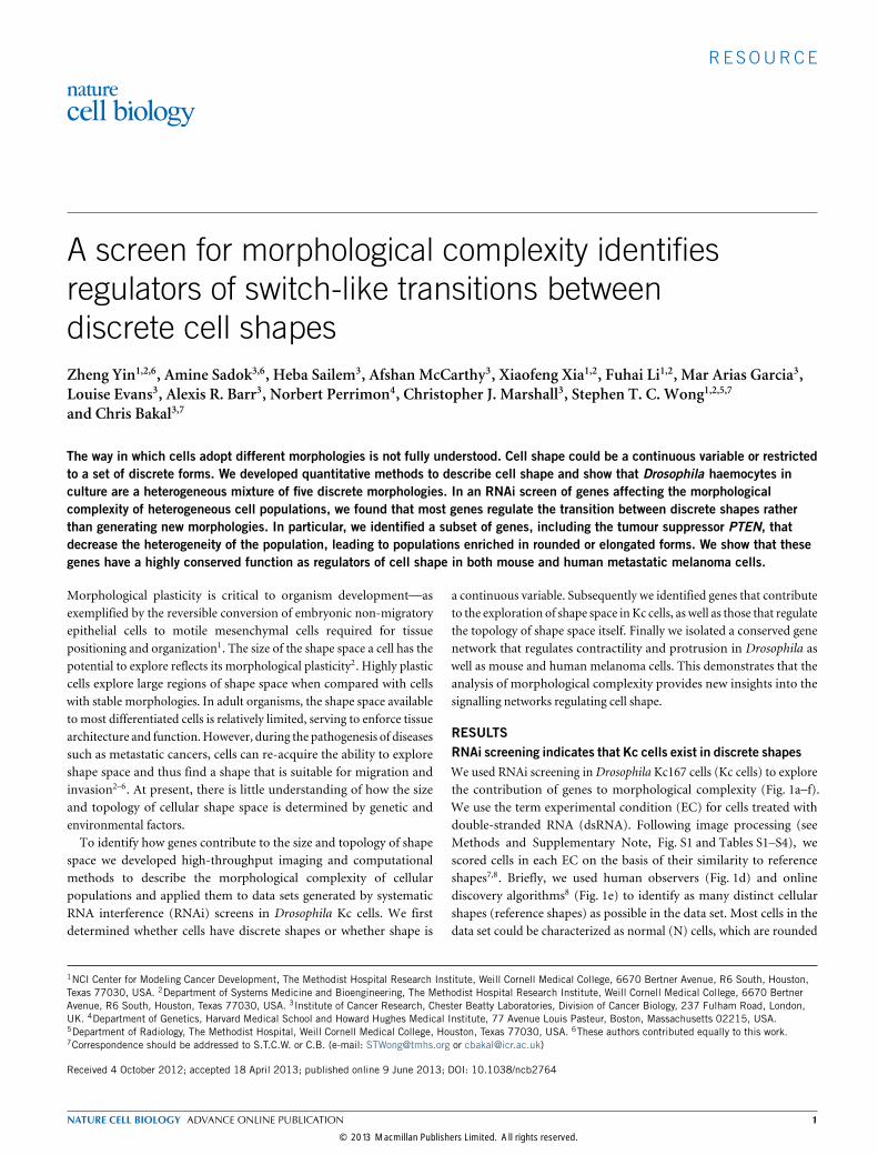
RESOURCE

A screen for morphological complexity identifiesregulators of switch-like transitions betweendiscrete cell shapesZheng Yin1,2,6, Amine Sadok3,6, Heba Sailem3, Afshan McCarthy3, Xiaofeng Xia1,2, Fuhai Li1,2, Mar Arias Garcia3,Louise Evans3, Alexis R. Barr3, Norbert Perrimon4, Christopher J. Marshall3, Stephen T. C. Wong1,2,5,7

and Chris Bakal3,7

The way in which cells adopt different morphologies is not fully understood. Cell shape could be a continuous variable or restrictedto a set of discrete forms. We developed quantitative methods to describe cell shape and show that Drosophila haemocytes inculture are a heterogeneous mixture of five discrete morphologies. In an RNAi screen of genes affecting the morphologicalcomplexity of heterogeneous cell populations, we found that most genes regulate the transition between discrete shapes ratherthan generating new morphologies. In particular, we identified a subset of genes, including the tumour suppressor PTEN, thatdecrease the heterogeneity of the population, leading to populations enriched in rounded or elongated forms. We show that thesegenes have a highly conserved function as regulators of cell shape in both mouse and human metastatic melanoma cells.

Morphological plasticity is critical to organism development—asexemplified by the reversible conversion of embryonic non-migratoryepithelial cells to motile mesenchymal cells required for tissuepositioning and organization1. The size of the shape space a cell has thepotential to explore reflects its morphological plasticity2. Highly plasticcells explore large regions of shape space when compared with cellswith stable morphologies. In adult organisms, the shape space availableto most differentiated cells is relatively limited, serving to enforce tissuearchitecture and function.However, during the pathogenesis of diseasessuch as metastatic cancers, cells can re-acquire the ability to exploreshape space and thus find a shape that is suitable for migration andinvasion2–6. At present, there is little understanding of how the sizeand topology of cellular shape space is determined by genetic andenvironmental factors.To identify how genes contribute to the size and topology of shape

space we developed high-throughput imaging and computationalmethods to describe the morphological complexity of cellularpopulations and applied them to data sets generated by systematicRNA interference (RNAi) screens in Drosophila Kc cells. We firstdetermined whether cells have discrete shapes or whether shape is

1NCI Center for Modeling Cancer Development, The Methodist Hospital Research Institute, Weill Cornell Medical College, 6670 Bertner Avenue, R6 South, Houston,Texas 77030, USA. 2Department of Systems Medicine and Bioengineering, The Methodist Hospital Research Institute, Weill Cornell Medical College, 6670 BertnerAvenue, R6 South, Houston, Texas 77030, USA. 3Institute of Cancer Research, Chester Beatty Laboratories, Division of Cancer Biology, 237 Fulham Road, London,UK. 4Department of Genetics, Harvard Medical School and Howard Hughes Medical Institute, 77 Avenue Louis Pasteur, Boston, Massachusetts 02215, USA.5Department of Radiology, The Methodist Hospital, Weill Cornell Medical College, Houston, Texas 77030, USA. 6These authors contributed equally to this work.7Correspondence should be addressed to S.T.C.W. or C.B. (e-mail: [email protected] or [email protected])

Received 4 October 2012; accepted 18 April 2013; published online 9 June 2013; DOI: 10.1038/ncb2764

a continuous variable. Subsequently we identified genes that contributeto the exploration of shape space in Kc cells, as well as those that regulatethe topology of shape space itself. Finally we isolated a conserved genenetwork that regulates contractility and protrusion in Drosophila aswell as mouse and human melanoma cells. This demonstrates that theanalysis of morphological complexity provides new insights into thesignalling networks regulating cell shape.

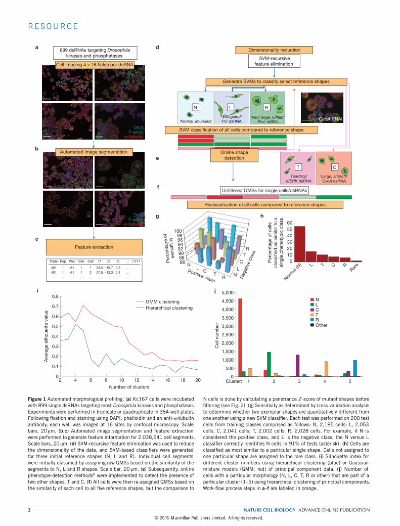
RESULTSRNAi screening indicates that Kc cells exist in discrete shapesWe used RNAi screening in Drosophila Kc167 cells (Kc cells) to explorethe contribution of genes to morphological complexity (Fig. 1a–f).We use the term experimental condition (EC) for cells treated withdouble-stranded RNA (dsRNA). Following image processing (seeMethods and Supplementary Note, Fig. S1 and Tables S1–S4), wescored cells in each EC on the basis of their similarity to referenceshapes7,8. Briefly, we used human observers (Fig. 1d) and onlinediscovery algorithms8 (Fig. 1e) to identify as many distinct cellularshapes (reference shapes) as possible in the data set. Most cells in thedata set could be characterized as normal (N) cells, which are rounded

NATURE CELL BIOLOGY ADVANCE ONLINE PUBLICATION 1

© 2013 Macmillan Publishers Limited. All rights reserved.

mailto:[email protected]

mailto:[email protected]

http://www.nature.com/doifinder/10.1038/ncb2764

RESOURCE

0

500

1,000

1,500

2,000

2,500

3,000

3,500

4,000

4,500

5,000

Feature extraction

899 dsRNAs targeting Drosophila

kinases and phosphatases

SVM-recursive

feature elimination

DNAF-actin

α-tubulin

Automated image segmentation

DNAF-actin

α-tubulin

Dimensionality reduction

0

10

20

30

40

50

60

Nor

mal (N

) L T C RRar

e

h

'Elongated'Pvr dsRNA'Normal' (rounded)

'Teardrop'rl/ERK dsRNA

'Very large, ruffled'Rho1 dsRNA

'Large, smooth'CycA dsRNA

CycA RNAi

LN R

T C

Generate SVMs to classify select reference shapes

Online shape

detection

Number of clusters

Avera

ge s

ilho

uett

e v

alu

e

Cluster: 1 2 3 4 5

NLCTROther

2 4 6 8 10 12 14 16 18 200

0.1

0.2

0.3

0.4

0.5

0.6

0.7

0.8

Hierarchical clustering

GMM clustering

j

10098969492908886

T

R

C

L

N

Perc

enta

ge o

f

sensitiv

ity

Positive class

Negative

cla

ss

LC

TR

N

∗

Cell imaging 4 × 16 fields per dsRNA

SVM classification of all cells compared to reference shape

Reclassification of all cells compared to reference shapes

Unfiltered QMSs for single cells/dsRNAs

Plate Rep Well Site Cell f1 f2 f3 ... f 211

401 1 A1 1 1 34.5 –19.7 0.2 ...

401 1 A1 1 2 27.5 –12.3 0.1 ...

... ... ... ... ... ... ... ... ...

Perc

en

tag

e o

f cells

cla

ssifie

d a

s s

imila

r to

a

sin

gle

ph

en

oty

pic

cla

ss

d

e

f

g

i

a

b

c

Cell

nu

mb

er

Figure 1 Automated morphological profiling. (a) Kc167 cells were incubatedwith 899 single dsRNAs targeting most Drosophila kinases and phosphatases.Experiments were performed in triplicate or quadruplicate in 384-well plates.Following fixation and staining using DAPI, phalloidin and an anti-α-tubulinantibody, each well was imaged at 16 sites by confocal microscopy. Scalebars, 20 µm. (b,c) Automated image segmentation and feature extractionwere performed to generate feature information for 2,038,641 cell segments.Scale bars, 20 µm. (d) SVM-recursive feature elimination was used to reducethe dimensionality of the data, and SVM-based classifiers were generatedfor three initial reference shapes (N, L and R). Individual cell segmentswere initially classified by assigning raw QMSs based on the similarity of thesegments to N, L and R shapes. Scale bar, 20 µm. (e) Subsequently, onlinephenotype-detection methods8 were implemented to detect the presence oftwo other shapes, T and C. (f) All cells were then re-assigned QMSs based onthe similarity of each cell to all five reference shapes, but the comparison to

N cells is done by calculating a penetrance Z -score of mutant shapes beforefiltering (see Fig. 2). (g) Sensitivity as determined by cross-validation analysisto determine whether two exemplar shapes are quantitatively different fromone another using a new SVM classifier. Each test was performed on 200 testcells from training classes comprised as follows: N, 2,185 cells; L, 2,053cells, C, 2,041 cells; T, 2,002 cells; R, 2,028 cells. For example, if N isconsidered the positive class, and L is the negative class, the N versus Lclassifier correctly identifies N cells in 91% of tests (asterisk). (h) Cells areclassified as most similar to a particular single shape. Cells not assigned toone particular shape are assigned to the rare class. (i) Silhouette index fordifferent cluster numbers using hierarchical clustering (blue) or Gaussianmixture models (GMM; red) of principal component data. (j) Number ofcells with a particular morphology (N, L, C, T, R or other) that are part of aparticular cluster (1–5) using hierarchical clustering of principal components.Work-flow process steps in a–f are labeled in orange.

2 NATURE CELL BIOLOGY ADVANCE ONLINE PUBLICATION


RESOURCE

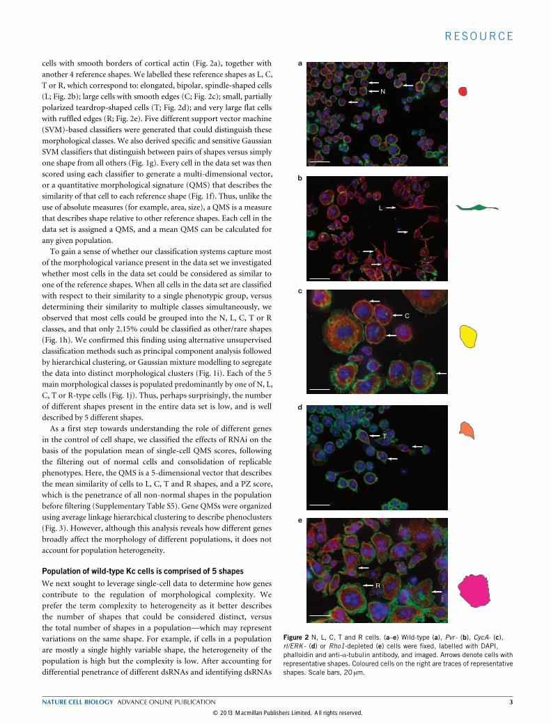
cells with smooth borders of cortical actin (Fig. 2a), together withanother 4 reference shapes. We labelled these reference shapes as L, C,T or R, which correspond to: elongated, bipolar, spindle-shaped cells(L; Fig. 2b); large cells with smooth edges (C; Fig. 2c); small, partiallypolarized teardrop-shaped cells (T; Fig. 2d); and very large flat cellswith ruffled edges (R; Fig. 2e). Five different support vector machine(SVM)-based classifiers were generated that could distinguish thesemorphological classes. We also derived specific and sensitive GaussianSVM classifiers that distinguish between pairs of shapes versus simplyone shape from all others (Fig. 1g). Every cell in the data set was thenscored using each classifier to generate a multi-dimensional vector,or a quantitative morphological signature (QMS) that describes thesimilarity of that cell to each reference shape (Fig. 1f). Thus, unlike theuse of absolute measures (for example, area, size), a QMS is a measurethat describes shape relative to other reference shapes. Each cell in thedata set is assigned a QMS, and a mean QMS can be calculated forany given population.To gain a sense of whether our classification systems capture most

of the morphological variance present in the data set we investigatedwhether most cells in the data set could be considered as similar toone of the reference shapes. When all cells in the data set are classifiedwith respect to their similarity to a single phenotypic group, versusdetermining their similarity to multiple classes simultaneously, weobserved that most cells could be grouped into the N, L, C, T or Rclasses, and that only 2.15% could be classified as other/rare shapes(Fig. 1h). We confirmed this finding using alternative unsupervisedclassification methods such as principal component analysis followedby hierarchical clustering, or Gaussian mixture modelling to segregatethe data into distinct morphological clusters (Fig. 1i). Each of the 5main morphological classes is populated predominantly by one of N, L,C, T or R-type cells (Fig. 1j). Thus, perhaps surprisingly, the numberof different shapes present in the entire data set is low, and is welldescribed by 5 different shapes.As a first step towards understanding the role of different genes

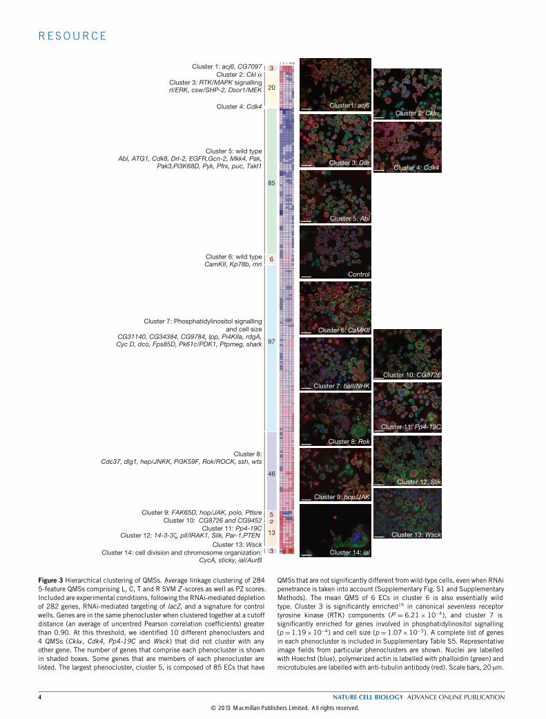
in the control of cell shape, we classified the effects of RNAi on thebasis of the population mean of single-cell QMS scores, followingthe filtering out of normal cells and consolidation of replicablephenotypes. Here, the QMS is a 5-dimensional vector that describesthe mean similarity of cells to L, C, T and R shapes, and a PZ score,which is the penetrance of all non-normal shapes in the populationbefore filtering (Supplementary Table S5). Gene QMSs were organizedusing average linkage hierarchical clustering to describe phenoclusters(Fig. 3). However, although this analysis reveals how different genesbroadly affect the morphology of different populations, it does notaccount for population heterogeneity.

Population of wild-type Kc cells is comprised of 5 shapesWe next sought to leverage single-cell data to determine how genescontribute to the regulation of morphological complexity. Weprefer the term complexity to heterogeneity as it better describesthe number of shapes that could be considered distinct, versusthe total number of shapes in a population—which may representvariations on the same shape. For example, if cells in a populationare mostly a single highly variable shape, the heterogeneity of thepopulation is high but the complexity is low. After accounting fordifferential penetrance of different dsRNAs and identifying dsRNAs

N

L

C

T

R

a

b

c

d

e

Figure 2 N, L, C, T and R cells. (a–e) Wild-type (a), Pvr - (b), CycA- (c),rl/ERK - (d) or Rho1-depleted (e) cells were fixed, labelled with DAPI,phalloidin and anti-α-tubulin antibody, and imaged. Arrows denote cells withrepresentative shapes. Coloured cells on the right are traces of representativeshapes. Scale bars, 20 µm.



RESOURCE

Cluster1: acj6

Cluster 1: acj6, CG7097

Cluster 2: CkI αCluster 3: RTK/MAPK signallingrl/ERK, csw/SHP-2, Dsor1/MEK

Cluster 4: Cdk4

Cluster 5: wild typeAbl, ATG1, Cdk8, Drl-2, EGFR,Gcn-2, Mkk4, Pak,

Pak3,Pi3K68D, Pyk, Pfrx, puc, Takl1

Cluster 8:Cdc37, dlg1, hep/JNKK, Pi3K59F, Rok/ROCK, ssh, wts

Cluster 7: Phosphatidylinositol signalling

and cell sizeCG31140, CG34384, CG9784, Ipp, Pi4KIIa, rdgA,Cyc D, dco, Fps85D, Pk61c/PDK1, Ptpmeg, shark

Cluster 9: FAK65D, hop/JAK, polo, Ptlsre

Cluster 10: CG8726 and CG9452

Cluster 11: Pp4-19CCluster 12: 14-3-3ζ, pll/IRAK1, Slik, Par-1,PTEN

Cluster 13: Wsck

Cluster 14: cell division and chromosome organization:CycA, sticky, ial/AurB

Cluster 2: CkIα

Cluster 4: Cdk4

Cluster 11: Pp4-19C

Cluster 13: Wsck

Cluster 8: Rok

Cluster 14: ial

Cluster 3: Ddr

Cluster 9: hop/JAK

Cluster 5: Abl

Cluster 7: ball/NHK

Cluster 6: CaMKII

Control

Cluster 6: wild typeCamKII, Kp78b, mri

Cluster 12: Slik

Cluster 10: CG8726

3

85

20

6

97

46

5

3

13

2

L C T R PZ

Figure 3 Hierarchical clustering of QMSs. Average linkage clustering of 2845-feature QMSs comprising L, C, T and R SVM Z -scores as well as PZ scores.Included are experimental conditions, following the RNAi-mediated depletionof 282 genes, RNAi-mediated targeting of lacZ, and a signature for controlwells. Genes are in the same phenocluster when clustered together at a cutoffdistance (an average of uncentred Pearson correlation coefficients) greaterthan 0.90. At this threshold, we identified 10 different phenoclusters and4 QMSs (CkIα, Cdk4, Pp4-19C and Wsck ) that did not cluster with anyother gene. The number of genes that comprise each phenocluster is shownin shaded boxes. Some genes that are members of each phenocluster arelisted. The largest phenocluster, cluster 5, is composed of 85 ECs that have

QMSs that are not significantly different from wild-type cells, even when RNAipenetrance is taken into account (Supplementary Fig. S1 and SupplementaryMethods). The mean QMS of 6 ECs in cluster 6 is also essentially wildtype. Cluster 3 is significantly enriched19 in canonical sevenless receptortyrosine kinase (RTK) components (P = 6.21× 10−4), and cluster 7 issignificantly enriched for genes involved in phosphatidylinositol signalling(p =1.19×10−4) and cell size (p =1.07×10−3). A complete list of genesin each phenocluster is included in Supplementary Table S5. Representativeimage fields from particular phenoclusters are shown. Nuclei are labelledwith Hoechst (blue), polymerized actin is labelled with phalloidin (green) andmicrotubules are labelled with anti-tubulin antibody (red). Scale bars, 20 µm.



RESOURCE

00

0.1

0.2

0.3

0.4

0.5

0.6

0.7

0.8

0.9

1.0

–2–6

26

–2–6

260

0.1

0.2

0.3

–1–3–5

1 3 5–2

–6

260

0.1

0.2

0.3

Cluster 5 (wild type)

PC2PC3

Den

sity

Cluster 8PC2PC3

Den

sity

d

Genes organized by phenocluster

Q s

co

re

Q(4)

All, Q(1)Within cluster, Q(2)

Other cluster, Q(3)

Similarity to other members of cluster

Similarity to all other ECsSimilarity to genes from other clusters

Q(2)

Q(1)

Q(3)

Distribution of all other ECs

Distribution of other ECs in phenocluster

Distribution of ECs from other clusters

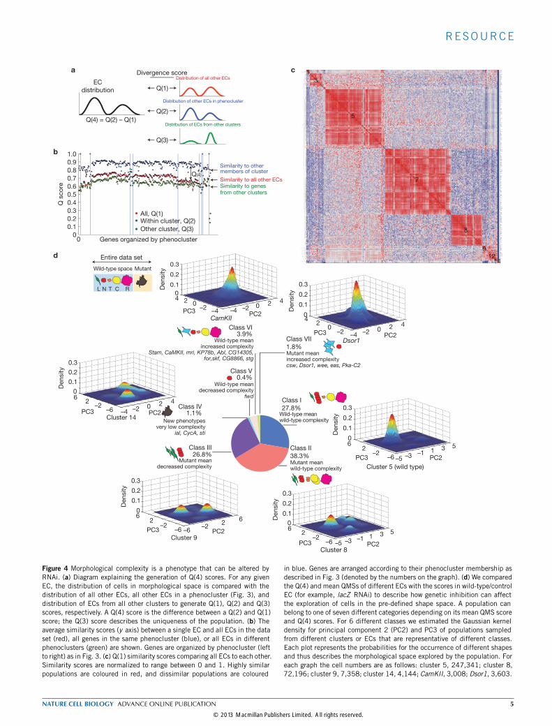
Divergence score

EC

distribution

a c

b

Entire data set

Wild-type space Mutant

Wild-type meanwild-type complexity

Mutant meanincreased complexitycsw, Dsor1, wee, eas, Pka-C2

New phenotypesvery low complexity

ial, CycA, sti

Wild-type meandecreased complexity

fwd

Wild-type meanincreased complexity

Stam, CaMKII, mri, KP78b, Abl, CG14305,for,skf, CG8866, stg

Cluster 9

Cluster 14

CamKII

Dsor1PC2PC3

Den

sity

PC2PC3

Den

sity

PC2PC3

Den

sity

PC2PC3

Den

sity

Mutant meanwild-type complexity

NL RT C

Class I

27.8%

Class II

38.3%

Class IV1.1%

Class V0.4%

Class VI3.9%

Class VII

1.8%

–1–3–51 3 5

–2–6

260

0.1

0.2

0.3

0–2–4

2 42–2

–6

60

0.1

0.2

0.3

0–2–4

2 40–2

240

0.1

0.2

0.3

0–2–42 40

–2–4

240

0.1

0.2

0.3

5

3

1

7

8

912

ialstiCycaWsvktrcCG15072SAKpar-1PtenPp2A–29BDgK14–3–3–zetCG32666CG7597cdc2rkpllslikPp4–19CCG9452CG8726Pp2B–14DPitslrehopFak26DpoloCG122252rokdlg1f(1) hPi3K59FIP3K2sshCG11440Gp150Cdc37Cad96CaCG32687flwweeNipped–APngPkg21DCG1906l(1)G0148PpD5CG7236Pka–C1Pez"fbI, CG339Sac1CG10999NeK2PapsauxillinCG9961CG8057tkvwtsCG11870CG14714Btk29ACG8789CG3290PTP–ERCG10417CG11221SNF1APp1alphaPp2C1hepCG10493Pka–C2Pk1–87BCG4629DoadrlCG7094CG11489lrbpPi4KIIalphaCG12169dppPPP4R2rTaf1Tak1CG3530CycGCG8179Ptp99ATao–1twsCG1697ballrgCG12151RetPpvCG31640CG7197CG3105PtpafuCakiCG9784CG6036CG7362rdgAlokCycdCG10376tweCycEGprk2PtmpegCG2577witCG9962Cdk7CG6805PEKAdk3PpD6Pkc98EmnbUnc–89CG5790CG5483CG14211IppPknCG14163msnCG4546CG4041mod (mdg4)slsSNF4AgamsaxCsksharkCycTCG11426CG31140"CG6355,CaMKICG2964CG31714CG5626ia2CG5144CG31187Strn–MlckMagiPp1–13CCG8286Fps85DCG4945Adk1Smg1NakCG8485dcodnkl (2) k01209KP78a"Mkp, CG3Pk61CStamCG14305mriCaMKIIsdtKP78bCycHPpN58APi3K68DEgfrSRPKAckslprCG32944CG9311CG10177Drl–2CG7156pucPk92BCG32703CG4839Pk34APk17EskfCG10089Gcn2PRL–1CG17124cdiArgkbtCG1227CG31711Ptp61GMkp3CG17746stgCG14030dntTakl1Pink1Cdk8AIkPhkgammaC–LaczLk6CycJPfrxPyKsgg"CG33671,CG11425nmoCdk5alphaPhImbtsmi35APP2A–B'WildtypePkgaurAtg1Mekk1Pak3Pka–C3pydPakI(1)G0232TieCG10459MbsSsICG3809nikiCG7134MadmMipp2fwdAdy43A1–2LarninaCCG12147MAPk–Ak2CG7115otkMkk4CG8866AbIforCdk4CanB2DdrCG12069CG10827SpreadCG6498aPKCDsor1cswCanA1Pka–R2Can–BPpY–55ACG7028CG10743Ptp4EMyt1CG18854rleasCklalphaacj6"CG18854,CG7097

14

Q(4) = Q(2) – Q(1)

26.8%Mutant mean

decreased complexity

Class III

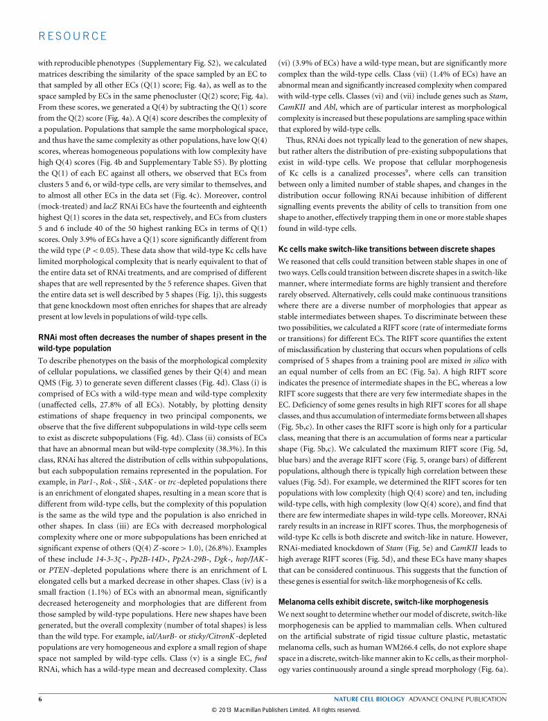
Figure 4 Morphological complexity is a phenotype that can be altered byRNAi. (a) Diagram explaining the generation of Q(4) scores. For any givenEC, the distribution of cells in morphological space is compared with thedistribution of all other ECs, all other ECs in a phenocluster (Fig. 3), anddistribution of ECs from all other clusters to generate Q(1), Q(2) and Q(3)scores, respectively. A Q(4) score is the difference between a Q(2) and Q(1)score; the Q(3) score describes the uniqueness of the population. (b) Theaverage similarity scores (y axis) between a single EC and all ECs in the dataset (red), all genes in the same phenocluster (blue), or all ECs in differentphenoclusters (green) are shown. Genes are organized by phenocluster (leftto right) as in Fig. 3. (c) Q(1) similarity scores comparing all ECs to each other.Similarity scores are normalized to range between 0 and 1. Highly similarpopulations are coloured in red, and dissimilar populations are coloured

in blue. Genes are arranged according to their phenocluster membership asdescribed in Fig. 3 (denoted by the numbers on the graph). (d) We comparedthe Q(4) and mean QMSs of different ECs with the scores in wild-type/controlEC (for example, lacZ RNAi) to describe how genetic inhibition can affectthe exploration of cells in the pre-defined shape space. A population canbelong to one of seven different categories depending on its mean QMS scoreand Q(4) scores. For 6 different classes we estimated the Gaussian kerneldensity for principal component 2 (PC2) and PC3 of populations sampledfrom different clusters or ECs that are representative of different classes.Each plot represents the probabilities for the occurrence of different shapesand thus describes the morphological space explored by the population. Foreach graph the cell numbers are as follows: cluster 5, 247,341; cluster 8,72,196; cluster 9, 7,358; cluster 14, 4,144; CamKII, 3,008; Dsor1, 3,603.



RESOURCE

with reproducible phenotypes (Supplementary Fig. S2), we calculatedmatrices describing the similarity of the space sampled by an EC tothat sampled by all other ECs (Q(1) score; Fig. 4a), as well as to thespace sampled by ECs in the same phenocluster (Q(2) score; Fig. 4a).From these scores, we generated a Q(4) by subtracting the Q(1) scorefrom the Q(2) score (Fig. 4a). A Q(4) score describes the complexity ofa population. Populations that sample the same morphological space,and thus have the same complexity as other populations, have low Q(4)scores, whereas homogeneous populations with low complexity havehigh Q(4) scores (Fig. 4b and Supplementary Table S5). By plottingthe Q(1) of each EC against all others, we observed that ECs fromclusters 5 and 6, or wild-type cells, are very similar to themselves, andto almost all other ECs in the data set (Fig. 4c). Moreover, control(mock-treated) and lacZ RNAi ECs have the fourteenth and eighteenthhighest Q(1) scores in the data set, respectively, and ECs from clusters5 and 6 include 40 of the 50 highest ranking ECs in terms of Q(1)scores. Only 3.9% of ECs have a Q(1) score significantly different fromthe wild type (P < 0.05). These data show that wild-type Kc cells havelimited morphological complexity that is nearly equivalent to that ofthe entire data set of RNAi treatments, and are comprised of differentshapes that are well represented by the 5 reference shapes. Given thatthe entire data set is well described by 5 shapes (Fig. 1j), this suggeststhat gene knockdown most often enriches for shapes that are alreadypresent at low levels in populations of wild-type cells.

RNAi most often decreases the number of shapes present in thewild-type populationTo describe phenotypes on the basis of the morphological complexityof cellular populations, we classified genes by their Q(4) and meanQMS (Fig. 3) to generate seven different classes (Fig. 4d). Class (i) iscomprised of ECs with a wild-type mean and wild-type complexity(unaffected cells, 27.8% of all ECs). Notably, by plotting densityestimations of shape frequency in two principal components, weobserve that the five different subpopulations in wild-type cells seemto exist as discrete subpopulations (Fig. 4d). Class (ii) consists of ECsthat have an abnormal mean but wild-type complexity (38.3%). In thisclass, RNAi has altered the distribution of cells within subpopulations,but each subpopulation remains represented in the population. Forexample, in Par1-, Rok-, Slik-, SAK - or trc-depleted populations thereis an enrichment of elongated shapes, resulting in a mean score that isdifferent from wild-type cells, but the complexity of this populationis the same as the wild type and the population is also enriched inother shapes. In class (iii) are ECs with decreased morphologicalcomplexity where one or more subpopulations has been enriched atsignificant expense of others (Q(4) Z -score> 1.0), (26.8%). Examplesof these include 14-3-3ζ -, Pp2B-14D-, Pp2A-29B-, Dgk-, hop/JAK -or PTEN -depleted populations where there is an enrichment of Lelongated cells but a marked decrease in other shapes. Class (iv) is asmall fraction (1.1%) of ECs with an abnormal mean, significantlydecreased heterogeneity and morphologies that are different fromthose sampled by wild-type populations. Here new shapes have beengenerated, but the overall complexity (number of total shapes) is lessthan the wild type. For example, ial/AurB- or sticky/CitronK -depletedpopulations are very homogeneous and explore a small region of shapespace not sampled by wild-type cells. Class (v) is a single EC, fwdRNAi, which has a wild-type mean and decreased complexity. Class

(vi) (3.9% of ECs) have a wild-type mean, but are significantly morecomplex than the wild-type cells. Class (vii) (1.4% of ECs) have anabnormal mean and significantly increased complexity when comparedwith wild-type cells. Classes (vi) and (vii) include genes such as Stam,CamKII and Abl, which are of particular interest as morphologicalcomplexity is increased but these populations are sampling space withinthat explored by wild-type cells.Thus, RNAi does not typically lead to the generation of new shapes,

but rather alters the distribution of pre-existing subpopulations thatexist in wild-type cells. We propose that cellular morphogenesisof Kc cells is a canalized processes9, where cells can transitionbetween only a limited number of stable shapes, and changes in thedistribution occur following RNAi because inhibition of differentsignalling events prevents the ability of cells to transition from oneshape to another, effectively trapping them in one ormore stable shapesfound in wild-type cells.

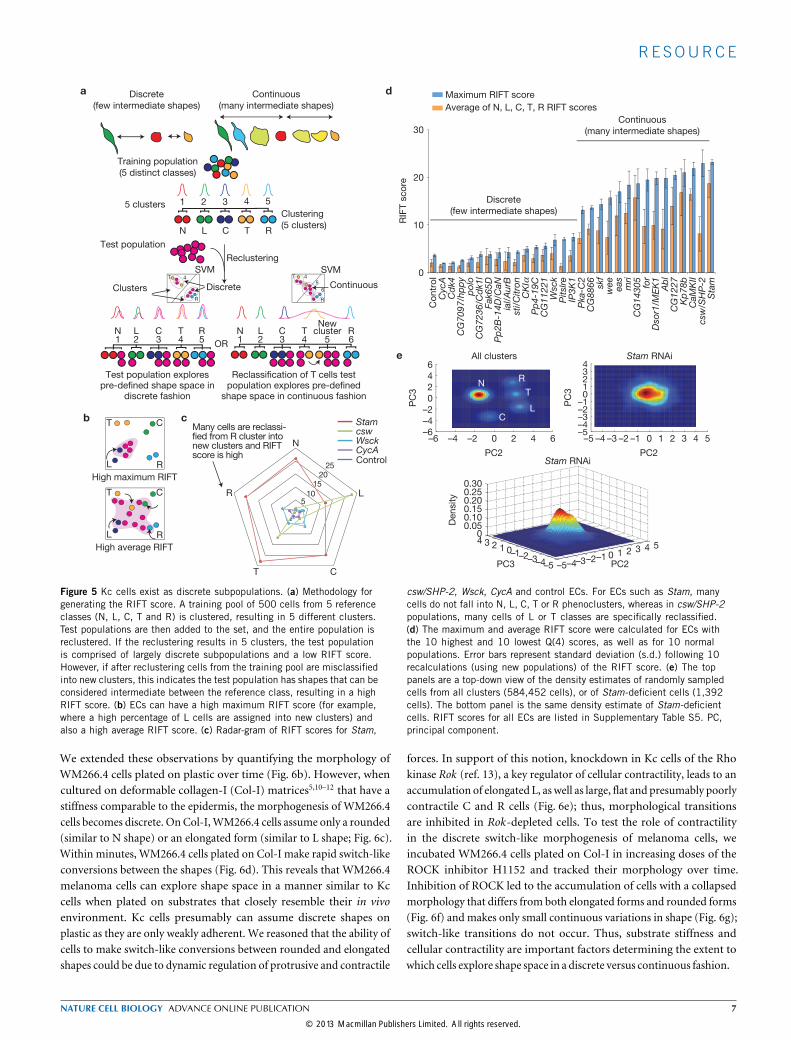
Kc cells make switch-like transitions between discrete shapesWe reasoned that cells could transition between stable shapes in one oftwo ways. Cells could transition between discrete shapes in a switch-likemanner, where intermediate forms are highly transient and thereforerarely observed. Alternatively, cells could make continuous transitionswhere there are a diverse number of morphologies that appear asstable intermediates between shapes. To discriminate between thesetwo possibilities, we calculated a RIFT score (rate of intermediate formsor transitions) for different ECs. The RIFT score quantifies the extentof misclassification by clustering that occurs when populations of cellscomprised of 5 shapes from a training pool are mixed in silico withan equal number of cells from an EC (Fig. 5a). A high RIFT scoreindicates the presence of intermediate shapes in the EC, whereas a lowRIFT score suggests that there are very few intermediate shapes in theEC. Deficiency of some genes results in high RIFT scores for all shapeclasses, and thus accumulation of intermediate forms between all shapes(Fig. 5b,c). In other cases the RIFT score is high only for a particularclass, meaning that there is an accumulation of forms near a particularshape (Fig. 5b,c). We calculated the maximum RIFT score (Fig. 5d,blue bars) and the average RIFT score (Fig. 5, orange bars) of differentpopulations, although there is typically high correlation between thesevalues (Fig. 5d). For example, we determined the RIFT scores for tenpopulations with low complexity (high Q(4) score) and ten, includingwild-type cells, with high complexity (low Q(4) score), and find thatthere are few intermediate shapes in wild-type cells. Moreover, RNAirarely results in an increase in RIFT scores. Thus, the morphogenesis ofwild-type Kc cells is both discrete and switch-like in nature. However,RNAi-mediated knockdown of Stam (Fig. 5e) and CamKII leads tohigh average RIFT scores (Fig. 5d), and these ECs have many shapesthat can be considered continuous. This suggests that the function ofthese genes is essential for switch-likemorphogenesis of Kc cells.

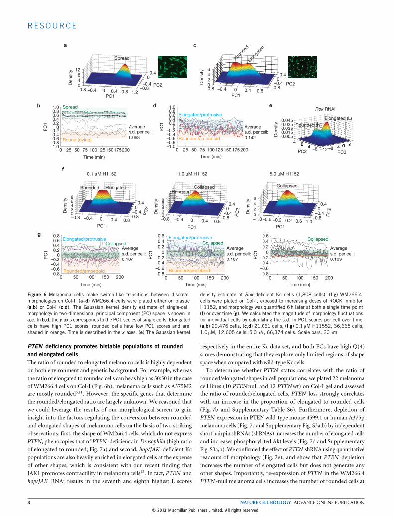
Melanoma cells exhibit discrete, switch-like morphogenesisWenext sought to determine whether ourmodel of discrete, switch-likemorphogenesis can be applied to mammalian cells. When culturedon the artificial substrate of rigid tissue culture plastic, metastaticmelanoma cells, such as human WM266.4 cells, do not explore shapespace in a discrete, switch-likemanner akin to Kc cells, as theirmorphol-ogy varies continuously around a single spread morphology (Fig. 6a).



RESOURCE

0–2–4–6 2 4 6

0

–2

–4

–6

2

4

6

PC

3

PC

3

PC2

1 2 3 4 5

N L C T R

Training population

(5 distinct classes)

Clustering

(5 clusters)

Test population

Reclustering

5 clusters

N L C T R1 2 3 4 5

Test population explorespre-defined shape space in

discrete fashion

d

OR

Newcluster

a

e

2520

15

105

L

C

R

N

T

StamcswWsckCycAControl

Many cells are reclassi-fied from R cluster intonew clusters and RIFTscore is high

N L C T R1 2 3 4 65

Discrete

(few intermediate shapes)

Discrete

(few intermediate shapes)

RIF

T s

co

re

Continuous

(many intermediate shapes)

T

R

45

6Continuous

T

R

4

5

SVM

DiscreteClusters

Sta

m

CaM

KII

Kp

78b

CG

14305

CG

1227

mri

csw

/SH

P-2

Ab

lD

so

r1/M

EK

1

eas

for

skf

wee

CG

8866

Pka-C

2IP

3K

1

Wsck

CG

11221

CK

IP

p4-1

9C

Pitslre

Fak65D

ial/A

urB

CG

7236/C

dk1l

Pp

2B

-14D

/CaN

sti/C

itro

n

Co

ntr

ol

po

lo

CycA

CG

7097/h

pp

yC

dk4

Continuous

(many intermediate shapes)

Maximum RIFT score

Average of N, L, C, T, R RIFT scores

T

R

C

L

T

R

C

L

High maximum RIFT

High average RIFT

b c

Reclassification of T cells testpopulation explores pre-defined

shape space in continuous fashion

0–1–2–3–4–5 1 2 3 4 5

0–1–2–3–4–5

1234

PC2

R

T

LC

N

SVM

PC2PC3

Density

0–1–2–3–4–5

1 2 3 4 50–1–2–3–4–5

12340

0.050.100.150.200.250.30

0

10

20

30

Stam RNAi

α

Stam RNAiAll clusters

Figure 5 Kc cells exist as discrete subpopulations. (a) Methodology forgenerating the RIFT score. A training pool of 500 cells from 5 referenceclasses (N, L, C, T and R) is clustered, resulting in 5 different clusters.Test populations are then added to the set, and the entire population isreclustered. If the reclustering results in 5 clusters, the test populationis comprised of largely discrete subpopulations and a low RIFT score.However, if after reclustering cells from the training pool are misclassifiedinto new clusters, this indicates the test population has shapes that can beconsidered intermediate between the reference class, resulting in a highRIFT score. (b) ECs can have a high maximum RIFT score (for example,where a high percentage of L cells are assigned into new clusters) andalso a high average RIFT score. (c) Radar-gram of RIFT scores for Stam,

csw/SHP-2, Wsck, CycA and control ECs. For ECs such as Stam, manycells do not fall into N, L, C, T or R phenoclusters, whereas in csw/SHP-2populations, many cells of L or T classes are specifically reclassified.(d) The maximum and average RIFT score were calculated for ECs withthe 10 highest and 10 lowest Q(4) scores, as well as for 10 normalpopulations. Error bars represent standard deviation (s.d.) following 10recalculations (using new populations) of the RIFT score. (e) The toppanels are a top-down view of the density estimates of randomly sampledcells from all clusters (584,452 cells), or of Stam-deficient cells (1,392cells). The bottom panel is the same density estimate of Stam-deficientcells. RIFT scores for all ECs are listed in Supplementary Table S5. PC,principal component.

We extended these observations by quantifying the morphology ofWM266.4 cells plated on plastic over time (Fig. 6b). However, whencultured on deformable collagen-I (Col-I) matrices5,10–12 that have astiffness comparable to the epidermis, the morphogenesis of WM266.4cells becomes discrete. OnCol-I,WM266.4 cells assume only a rounded(similar to N shape) or an elongated form (similar to L shape; Fig. 6c).Within minutes, WM266.4 cells plated on Col-I make rapid switch-likeconversions between the shapes (Fig. 6d). This reveals that WM266.4melanoma cells can explore shape space in a manner similar to Kccells when plated on substrates that closely resemble their in vivoenvironment. Kc cells presumably can assume discrete shapes onplastic as they are only weakly adherent. We reasoned that the ability ofcells to make switch-like conversions between rounded and elongatedshapes could be due to dynamic regulation of protrusive and contractile

forces. In support of this notion, knockdown in Kc cells of the Rhokinase Rok (ref. 13), a key regulator of cellular contractility, leads to anaccumulation of elongated L, as well as large, flat and presumably poorlycontractile C and R cells (Fig. 6e); thus, morphological transitionsare inhibited in Rok-depleted cells. To test the role of contractilityin the discrete switch-like morphogenesis of melanoma cells, weincubated WM266.4 cells plated on Col-I in increasing doses of theROCK inhibitor H1152 and tracked their morphology over time.Inhibition of ROCK led to the accumulation of cells with a collapsedmorphology that differs from both elongated forms and rounded forms(Fig. 6f) and makes only small continuous variations in shape (Fig. 6g);switch-like transitions do not occur. Thus, substrate stiffness andcellular contractility are important factors determining the extent towhich cells explore shape space in a discrete versus continuous fashion.



RESOURCE

0246

PC2

PC1

Den

sity

c

d

5.0 µM H1152

–1.0 –0.6 –0.2 0.2 0.6 1.0

0

2

4

6

Den

sity

PC2

.

1.0 µM H1152

02468

Den

sity

PC2

–0.8 –0.4 0 0.4 0.8–0.8

–0.40

0.4

–0.8 –0.4 0 0.4 0.8-0.8-0.4

0.40

–0.8–0.4

0.40

PC1 PC1

b

Round (dying)

0–0.2–0.4–0.6–0.8–1.0

0.20.40.60.81.0

PC

1

Spread

Elongated/protrusive

Rounded/amoeboid

0–0.2–0.4–0.6–0.8–1.0

0.20.40.60.81.0

0 25 50 75 100125150175200

Time (min)

0 25 50 75 100125150175200

Time (min)P

C1

Rounded/amoeboid

Elongated/protrusive

Average

s.d. per cell:

0.142

Collapsed

Average

s.d. per cell:

0.068

048

12

PC2

PC1

Den

sity

a

–0.8–0.4

00.4

–0.8 –0.4 0 0.4 0.8 1.2

Spread Rou

nded

Elong

ated

f

g

0.1 µM H1152

PC

2

PC

2

PC

2

PC1

–0.8 –0.4 0 0.4 0.8

02468

Den

sity

–0.8–0.4

0.40

–0.8–0.6–0.4–0.2

00.20.40.60.8

0 50 100 150 200

Time (min)

0 50 100 150 200

Time (min)

0 50 100 150 200

Time (min)

PC

1

–0.8–0.6–0.4–0.2

00.20.40.6

PC

1

–0.8–0.6–0.4–0.2

00.20.40.6

PC

1

Average

s.d. per cell:

0.107

Average

s.d. per cell:

0.107

Average

s.d. per cell:

0.109

RoundedRounded Collapsed Collapsed

eRok RNAi

0–4–8–124

–4 –8

40.0050.0150.0250.0350.045

PC3PC2

Den

sity

Elongated (L)

Rounded (N)

CollapsedCollapsedElongated/protrusive

Elongated

Rounded/amoeboid

Figure 6 Melanoma cells make switch-like transitions between discretemorphologies on Col-I. (a–d) WM266.4 cells were plated either on plastic(a,b) or Col-I (c,d). The Gaussian kernel density estimate of single-cellmorphology in two-dimensional principal component (PC) space is shown ina,c. In b,d, the y axis corresponds to the PC1 scores of single cells. Elongatedcells have high PC1 scores; rounded cells have low PC1 scores and areshaded in orange. Time is described in the x axes. (e) The Gaussian kernel

density estimate of Rok -deficient Kc cells (1,808 cells). (f,g) WM266.4cells were plated on Col-I, exposed to increasing doses of ROCK inhibitorH1152, and morphology was quantified 6h later at both a single time point(f) or over time (g). We calculated the magnitude of morphology fluctuationsfor individual cells by calculating the s.d. in PC1 scores per cell over time.(a,b) 29,476 cells, (c,d) 21,061 cells, (f,g) 0.1 µM H11552, 36,665 cells;1.0 µM, 12,605 cells; 5.0 µM, 66,374 cells. Scale bars, 20 µm.

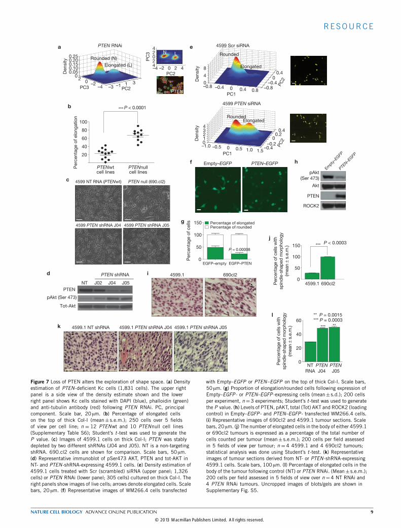
PTEN deficiency promotes bistable populations of roundedand elongated cellsThe ratio of rounded to elongated melanoma cells is highly dependenton both environment and genetic background. For example, whereasthe ratio of elongated to rounded cells can be as high as 50:50 in the caseof WM266.4 cells on Col-I (Fig. 6b), melanoma cells such as A375M2are mostly rounded5,11. However, the specific genes that determinethe rounded/elongated ratio are largely unknown. We reasoned thatwe could leverage the results of our morphological screen to gaininsight into the factors regulating the conversion between roundedand elongated shapes of melanoma cells on the basis of two strikingobservations: first, the shape of WM266.4 cells, which do not expressPTEN, phenocopies that of PTEN -deficiency in Drosophila (high ratioof elongated to rounded; Fig. 7a) and second, hop/JAK -deficient Kcpopulations are also heavily enriched in elongated cells at the expenseof other shapes, which is consistent with our recent finding thatJAK1 promotes contractility in melanoma cells12. In fact, PTEN andhop/JAK RNAi results in the seventh and eighth highest L scores

respectively in the entire Kc data set, and both ECs have high Q(4)scores demonstrating that they explore only limited regions of shapespace when compared with wild-type Kc cells.To determine whether PTEN status correlates with the ratio of

rounded/elongated shapes in cell populations, we plated 22 melanomacell lines (10 PTENnull and 12 PTENwt) on Col-I gel and assessedthe ratio of rounded/elongated cells. PTEN loss strongly correlateswith an increase in the proportion of elongated to rounded cells(Fig. 7b and Supplementary Table S6). Furthermore, depletion ofPTEN expression in PTEN wild-type mouse 4599.1 or human A375pmelanoma cells (Fig. 7c and Supplementary Fig. S3a,b) by independentshort hairpin shRNAs (shRNAs) increases the number of elongated cellsand increases phosphorylated Akt levels (Fig. 7d and SupplementaryFig. S3a,b).We confirmed the effect of PTEN shRNA using quantitativereadouts of morphology (Fig. 7e), and show that PTEN depletionincreases the number of elongated cells but does not generate anyother shapes. Importantly, re-expression of PTEN in the WM266.4PTEN -null melanoma cells increases the number of rounded cells at



RESOURCE

0–0.4–0.80.4 0.8

–0.8–0.4

00.4

0

4

8

4599 Scr siRNA

Rounded

Elongated

0 0.5–0.5–1.01.0 1.5

–0.4–0.2

00.2

0.4

01234

4599 PTEN siRNA

4599 NT RNA (PTENwt)

4599 PTEN shRNA J054599 PTEN shRNA J04

PTEN null (690.cl2)

pAkt (Ser 473)

NT

Tot-Akt

P < 0.0001

20

40

60

80

100

***

Perc

enta

ge o

f elo

ng

atio

n

a

c

d

J02 J04 J05

PTEN shRNA

f

g

Empty–EGFP PTEN–EGFP

i 4599.1 690cl2

k

l

4599.1 NT shRNA 4599.1 PTEN shRNA J04 4599.1 PTEN shRNA J05

0

20

40

60*****

Perc

enta

ge o

f cells

with

sp

ind

le-s

hap

ed

morp

holo

gy

(mean ±

s.e

.m.)

NT

RNA

PTEN

J04

PTEN

J05

** P = 0.0015*** P = 0.0003

e

h

j

PTEN

0

50

100

150 Percentage of elongatedPercentage of rounded

P = 0.00008

Perc

enta

ge o

f cells

EGFP–PTENEGFP–empty

Empty

–EGFP

PTEN–E

GFP

pAkt

(Ser 473)

Akt

PTEN

ROCK2

Perc

enta

ge o

f cells

with

sp

ind

le-s

hap

ed

morp

holo

gy

(mean ±

s.e

.m.)

0

50

100

150 ***P < 0.0003

4599.1 690cl2

RoundedElongated

PC2PC3 –1–31 30

–22

00.050.100.150.200.25

Density Rounded (N)

Elongated (L)

PTEN RNAi

0–4 –2 2 4

024

24

PC2

PC

3 N L

PTEN

Density

Density

b

PC1

PC1

PC

2P

C2

PTENwtcell lines

PTENnullcell lines

–4

Figure 7 Loss of PTEN alters the exploration of shape space. (a) Densityestimation of PTEN -deficient Kc cells (1,831 cells). The upper rightpanel is a side view of the density estimate shown and the lowerright panel shows Kc cells stained with DAPI (blue), phalloidin (green)and anti-tubulin antibody (red) following PTEN RNAi. PC, principalcomponent. Scale bar, 20 µm. (b) Percentage of elongated cellson the top of thick Col-I (mean± s.e.m.); 250 cells over 5 fieldsof view per cell line; n = 12 PTENwt and 10 PTENnull cell lines(Supplementary Table S6); Student’s t -test was used to generate theP value. (c) Images of 4599.1 cells on thick Col-I; PTEN was stablydepleted by two different shRNAs (J04 and J05). NT is a non-targetingshRNA. 690.cl2 cells are shown for comparison. Scale bars, 50 µm.(d) Representative immunoblot of pSer473 AKT, PTEN and tot-AKT inNT- and PTEN -shRNA-expressing 4599.1 cells. (e) Density estimation of4599.1 cells treated with Scr (scrambled) siRNA (upper panel; 1,326cells) or PTEN RNAi (lower panel; 305 cells) cultured on thick Col-I. Theright panels show images of live cells; arrows denote elongated cells. Scalebars, 20 µm. (f) Representative images of WM266.4 cells transfected

with Empty–EGFP or PTEN–EGFP on the top of thick Col-I. Scale bars,50 µm. (g) Proportion of elongation/rounded cells following expression ofEmpty–EGFP - or PTEN–EGFP -expressing cells (mean± s.d.); 200 cellsper experiment, n=3 experiments; Student’s t -test was used to generatethe P value. (h) Levels of PTEN, pAKT, total (Tot) AKT and ROCK2 (loadingcontrol) in Empty–EGFP - and PTEN–EGFP - transfected WM266.4 cells.(i) Representative images of 690cl2 and 4599.1 tumour sections. Scalebars, 20 µm. (j) The number of elongated cells in the body of either 4599.1or 690cl2 tumours is expressed as a percentage of the total number ofcells counted per tumour (mean± s.e.m.); 200 cells per field assessedin 5 fields of view per tumour; n = 4 4599.1 and 4 690cl2 tumours;statistical analysis was done using Student’s t -test. (k) Representativeimages of tumour sections derived from NT- or PTEN -shRNA-expressing4599.1 cells. Scale bars, 100 µm. (l) Percentage of elongated cells in thebody of the tumour following control (NT) or PTEN RNAi. (Mean± s.e.m.);200 cells per field assessed in 5 fields of view over n =4 NT RNAi and4 PTEN RNAi tumours. Uncropped images of blots/gels are shown inSupplementary Fig. S5.



RESOURCE

Group 1

Pro-elongation

Negative inhibitors

of elongation Positive regulators

of rounding

Group 2

Pro-rounding

MAPK1

MAPK3

IRAK1

JAK1

PAR-114-3-3ζ

PTEN

PLK1DIP1

EphrinAFHOD2gp130IL-6

LIMK1MYL2PAK2PDK1RhoCSTAT3

Stathmin1

CrkLDOCK3

Integrin β1LIMK2

p27Kip1p53

p130CasNEDD9MyoPRab5RhoE

SMURF2Src

WASF2

MAST 1/2

SLK LOK

Liprin-B2

Cdk10Cdk4

NT IRAK1 SLK PLK1

45

99

.1A

37

5p

a

b

d

c

NT

IRAK1

MAR

K2SLK Lo

kPLK

14-3

-3

CDK10

CDK4

Liprin

1

Liprin

2

PKMYT1

Ek1/2

MAST1

MAST2

MAST3 N

T

IRAK1

MAR

K2SLK Lo

kPLK

CDK10

CDK4

PKMYT1

Ek1/2

MAST1

MAST2

MAST3

0

20

40

60

80

Perc

en

tag

e o

f elo

ng

atio

n

0

20

40

60

80

Perc

en

tag

e o

f elo

ng

atio

n

******

***

*

***

** ** **

**

*****

**

**

nsns

***

***

******

**

**

ns ns ns ns

ns ns ns

*

4599.1 A375p

β βζ

14-3

-3ζ

Liprin

1

Liprin

2β β

Figure 8 A conserved set of genes promotes rounding in Drosophila, mouseand human cells. (a) Mouse 4599.1 (upper panels) and human A375p (lowerpanels) metastatic melanoma cells plated on Col-I following RNAi-mediatedgene knockdown of IRAK1, SLK and PLK1. NT is non-targeting RNAi. Scalebars, 50 µm. (b) Percentage of elongated cells following knockdown of 15mouse genes in 4599.1 cells plated on Col-I (mean± s.e.m.). (c) Percentageof elongated cells following knockdown of 15 human genes in A375p cellsplated on Col-I (mean± s.e.m.). In b,c, 250 cells over n = 3 experiments.Student’s t -test was used to generate the P values. The asterisks denote thelevel of significance: ∗P < 0.05, ∗∗P < 0.001, ∗∗∗P < 0.0001. (d) Networkanalysis. We calculated the proximity of different proteins identified in our

screen to either pro-elongation proteins or pro-rounding proteins in theprotein–protein interaction space. The length of the arrow is scaled to aZ -score that describes the significance of this proximity compared withrandom proteins, where longer arrows are less significant and thus furtheraway in the protein–protein interaction space. As inhibition of all proteinshere results in elongated shapes, we could classify different proteins asnegative regulators of elongation or positive regulators of rounding. Proteinsin the pale orange rectangle are not significantly close to either group. Greencircles indicate that gene depletion increases the percentage of elongationin mouse and human cells; the yellow circles indicate that gene depletionincreases the percentage of elongation in mouse cells.



RESOURCE

the expense of elongated cells (Fig. 7f–h). To determine whether PTENregulates the exploration of shape space in vivo we used orthotopicimplantation of melanoma cells from 4599.1 cells (PTENwt), 4599.1cell populations stably expressing two different PTEN shRNAs or690cl2 (PTENnull) into the dermis of NOD SCID mice and assessedthe shape in haematoxylin and eosin-stained sections5,14. Tumourcells arising from injection of 4599.1 cells are predominantly rounded(Fig. 6i,j) whereas tumour cells arising from injection of 690cl2 cells(Fig. 7i,j), or 4599.1 cells in which PTEN had been knocked down, aremarkedly elongated (Fig. 7k,l and Supplementary Fig. S4). Thus, PTENloss induces elongation cells in tissue culture and in vivo.

A conserved class of genes that promote cell roundingGiven that depletion of PTEN and JAK results in bistable populationsof elongated and rounded cells in Drosophila, mouse and human cells,we sought to determine whether other genes identified in theDrosophilascreen are conserved regulators of morphogenesis. We selected geneswhose depletion in Drosophila cells results in a significant increasein the number of elongated cells, or the magnitude of their L scores(Supplementary Table S7). Genes were further prioritized if theirinhibition resulted in low complexity (high Q(4) score), and thuswere enriched in L cells at the expense of other shapes. For example,whereas PLK1- and 14-3-3ζ -depleted Drosophila cell populationsare comprised almost exclusively of rounded and elongated shapes,Slik-depleted populations have a high (L) score, but are also enrichedin other subpopulations. We tested only genes where we could identifyhuman homologues; in some cases this required targeting of multiplegenes (for example,MAST1,MAST2 andMAST3 are homologues ofDrosophila CG6498; Supplementary Table S7). Using short interferingRNA (siRNA) pools (Supplementary Tables S8 and S9) we depleted15 different homologues of 11 different Drosophila genes in 4599.1mouse and A375p human melanoma cells. When cultured in starvingconditions on a thick Col-I matrix, both 4599.1 and A375p convertto elongated cells at a low frequency; we scored populations onthe basis of whether siRNA knockdown increases the frequency ofelongation (Fig. 8a). RNAi-mediated knockdown of 12/15 genes inmouse (Fig. 8b) and 7/15 genes human cells results in significantincreases in elongation that phenocopy their depletion in Drosophila(Supplementary Table S7). For example, depletion of mouse andhuman IRAK1, PLK1, PTEN, ERK1 and ERK2 led to marked increasesin the numbers of elongated cells (Fig. 8b). That 10/11 Drosophilagenes whose depletion results in a high L score can be validated asregulators of cell rounding in at least one mammalian metatstaticmelanoma tumour line, in addition to PTEN and JAK, highlightsthe ability of our RNAi screen to identify genes that have relevanceto disease progression.

Classifying genes as protrusion antagonists or contractilityagonistsTowards gaining systems-level mechanistic insights into how differentvalidated genes identified in our screen regulate cell shape, weperformed a network analysis to determine the proximity ofdifferent proteins in network space to regulators of protrusivenessor contractility. Proteins previously implicated in controlling cell shapewere classified into either pro-elongation or pro-contractility groups15.We then calculated the average number of edges that separated

proteins identified in our screen from proteins in either previouslyassigned group in protein–protein interaction networks, and judgedthe significance of this distance compared with that between otherrandom proteins. Proteins such as JAK1 and IRAK1 are significantlycloser in protein–protein interaction space to the pro-contractilitygroup, whereas PTEN and 14−3−3ζ are closer to the pro-elongationgroup (Fig. 8d). Given that depletion of all these genes results insimilar elongated shapes, we conclude that JAK1 and IRAK1 promoterounding, but 14− 3− 3ζ and PTEN negatively inhibit protrusion.This unbiased network is consistent with our previous observation thatJAK1 upregulates contractility by activation of the STAT3 transcriptionfactor12, and that PTEN is a negative regulator of PI(3)K that actsto promote protrusion in multiple other cell types16. Interestingly,proteins such as ERK1/2 have not been previously associated with anupregulation of contractility. Thus, this analysis provides hypothesesfor other poorly characterized genes.

DISCUSSIONBy implementing methods to quantify mean morphology, complexityand presence of intermediate forms in cell populations in an RNAiscreen of Drosophila Kc cells, we propose that cells can explore shapespace in a discrete, switch-likemanner. Using live-cell imagingmethodsin combination with morphological quantification, we demonstratethat this type ofmorphogenesis is not limited toDrosophila haemocytes,and that metastatic melanoma cells explore shape space in a similarfashion when plated on substrates that mimic their in vivo environment.We propose that many cell types will also exhibit discrete switch-likemorphogenesis in vivo, and that it has been the long-standing useof rigid tissue culture plastic that has obscured this aspect of cellshape control. Although the model that cells can be constrained tospecific regions of shape space is potentially counter-intuitive giventhe highly plastic nature of cell shape and the ability of cells to adoptradically diverse shapes, discrete morphogenesis or morphologicalcanalization of single cells17 is consistent with the idea that signallingnetworks are dynamic systems that can exist in a limited number ofstable states, or attractors18.That systematic gene inhibition by RNAi can alter shape space

and/or alter themode ofmorphogenesis from switch-like to continuous(for example, Stam RNAi), suggests that signalling networks haveevolved to couple the topology of their shape space, and how theyexplore it, to environmental conditions. Metastatic cancer cells mayhave re-engineered regulatory networks that uncouple the controlof morphogenesis from environmental cues, which would otherwisedictate the number of shapes they can assume and how they convertbetween these shapes. In the case of PTEN, it is tempting to speculatethat loss of PTEN may promote the adoption of a bistable statewhere rounded and elongated forms are present in high numbers. Byincreasing the frequency of rounded and elongated cells this wouldprovide metastatic cells with a survival advantage that is otherwise notgained by adopting only a single shape, or being highly plastic. �

METHODSMethods and any associated references are available in the onlineversion of the paper.

Note: Supplementary Information is available in the online version of the paper






RESOURCE

ACKNOWLEDGEMENTSWe are indebted to the Drosophila RNAi Screening Center staff at Harvard MedicalSchool for their invaluable assistance. We especially thank I. Flockhart for assistancewith data management. We thank J. Wang, X. Zhou and P. Bradley for theirinitial involvement in this study. We are grateful to N. Dhomen and R. Marais formelanoma cell lines. Work was financially supported in part by NCI grants (GrantsR01CA121225 and U54CA149196) to S.T.C.W. and CRUK grants to C.B. (Grant13478) and C.J.M. (Grant C107/A10433). N.P. is an Investigator of the HowardHughes Medical Institute. A.S. is a Marie Curie Intra-European Fellow. C.J.M. isa Gibb Life Fellow of CRUK. C.B. is a Research Career Development Fellow of theWellcome Trust.

AUTHOR CONTRIBUTIONSZ.Y. performed the bulk of statistical analysis of RNAi screening data and wrotethe Supplementary Note. A.S. designed and performed all RNAi and cell linecharacterization experiments in mouse and humanmelanoma cells and contributedto writing of the manuscript. H.S. performed the analysis of live-cell melanomacell imaging experiments and contributed to visualization of statistical results.A.M. performed all mouse work. X.X. and F.L. performed processing of imagesgenerated in Drosophila RNAi screen. M.A.G. and L.E. performed experimentsdescribing penetrance of effects of different dsRNAs. A.R.B. contributed to writingand editing of the manuscript and the Supplementary Note. N.P. participated inthe initial design of the study. S.T.C.W. coordinated image processing and statisticalanalysis. C.J.M. participated in design of melanoma experiments and contributedto writing the manuscript. C.B. participated in the design of experiments andstatistical analysis, performed the Drosophila RNAi screen, performed the live-cellimaging assays, coordinated experimental and computational analysis, and wrotethe manuscript.

COMPETING FINANCIAL INTERESTSThe authors declare no competing financial interests.

Published online at www.nature.com/doifinder/10.1038/ncb2764Reprints and permissions information is available online at www.nature.com/reprints

1. Thiery, J.P., Acloque, H., Huang, R. Y. & Nieto, M. A. Epithelial-mesenchymaltransitions in development and disease. Cell 139, 871–890 (2009).

2. Keren, K. et al. Mechanism of shape determination in motile cells. Nature 453,475–480 (2008).

3. Mogilner, A. & Keren, K. The shape of motile cells. Curr. Biol. 19,R762–R771 (2009).

4. Guarino, M., Rubino, B. & Ballabio, G. The role of epithelial-mesenchymal transitionin cancer pathology. Pathology 39, 305–318 (2007).

5. Sanz-Moreno, V. et al. Rac activation and inactivation control plasticity of tumourcell movement. Cell 135, 510–523 (2008).

6. Wolf, K. et al. Compensation mechanism in tumour cell migration: mesenchymal-amoeboid transition after blocking of pericellular proteolysis. J. Cell Biol. 160,267–277 (2003).

7. Bakal, C., Aach, J., Church, G. & Perrimon, N. Quantitative morphologicalsignatures define local signalling networks regulating cell morphology. Science 316,1753–1756 (2007).

8. Yin, Z. et al. Using iterative cluster merging with improved gap statistics to performonline phenotype discovery in the context of high-throughput RNAi screens. BMCBioinformatics 9, 264 (2008).

9. Waddington, C. H. The Strategy of Genes (Allen Unwin, 1957).10. Gadea, G., Sanz-Moreno, V., Self, A., Godi, A. & Marshall, C. J. DOCK10-mediated

Cdc42 activation is necessary for amoeboid invasion of melanoma cells. Curr. Biol.18, 1456–1465 (2008).

11. Sahai, E. & Marshall, C. J. Differing modes of tumour cell invasion have distinctrequirements for Rho/ROCK signalling and extracellular proteolysis. Nat. Cell Biol.5, 711–719 (2003).

12. Sanz-Moreno, V. et al. ROCK and JAK1 signalling cooperate to controlactomyosin contractility in tumour cells and stroma. Cancer Cell 20,229–245 (2011).

13. Tan, C., Stronach, B. & Perrimon, N. Roles of myosin phosphatase during Drosophiladevelopment. Development 130, 671–681 (2003).

14. Viros, A. et al. Improving melanoma classification by integrating genetic andmorphologic features. PLoS Med. 5, e120 (2008).

15. Sanz-Moreno, V. & Marshall, C. J. The plasticity of cytoskeletal dynamics underlyingneoplastic cell migration. Curr. Opin. Cell Biol. 22, 690–696 (2010).

16. Ridley, A. J. et al. Cell migration: integrating signals from front to back. Science302, 1704–1709 (2003).

17. Waddington, C. H. Canalization of development and genetic assimilation of acquiredcharacters. Nature 183, 1654–1655 (1959).

18. Kauffman, S. A. The Origins of Order. Self-Organization and Selection in Evolution(Oxford Univ. Press, 1993).

19. Dhomen, N. et al. Oncogenic Braf induces melanocyte senescence and melanomain mice. Cancer Cell 15, 294–303 (2009).




http://www.nature.com/reprints

DOI: 10.1038/ncb2764 METHODS

METHODSCell culture, plasmids and RNAi transfection. A375p and A375M2 cells werefrom R. Hynes (Howard Hughes Medical Institute, Massachusetts Institute of Tech-nology, USA).WM266.4, LU1205,WM1361 andWM1366 cells were fromR.Marais(Paterson Institute, Manchester, UK), SKMEL24 cells were from ATCC, andWM239 cells were fromW. Cruz and R. Kerbel (Sunnybrook Health Science Centre,Toronto, Canada). 690cl2, 7491cl1, 690cl5, 690cl6, 4434cl2, 5537, 1840cl5, 5021cl6,2225, 5017, A061 and 4599 cells were generated by N. Dhomen and R. Marais (Pa-terson Institute, Manchester, USA) either from tumours arising in the Braf V600Emouse model20 or from tumours arising from the BrafV600E PTEN-null mousemelanoma tumour model21. We have generated the AM997-2 and AM993-1 linesfrom the BRAFV600E/PTENnull mouse melanoma tumour model. All of the cellswere maintained in DMEM containing 10% fetal calf serum. Human GFP–PTENwas from Addgene (Plasmid #13039). Plasmid transfection was performed withLipofectamine 2000 (Invitrogen) according to the manufacturer’s protocol. TheOn-TARGETplus siRNAs against human PTEN and the On-TARGETplus set of4 siRNAs against mouse PTEN were from Dharmacon (Supplementary TableS8). For other siRNA experiments targeting genes other than PTEN when usedOn-TARGETplus pools (Dharmacon). Transfection was performed with RNAimaxLipofectamine (Invitrogen) according to the manufacturer’s protocol.

Drosophila Kc167 cells were cultured in Schneider’s insect media (Invitrogen),10% fetal bovine serum (Invitrogen) and penicillin/streptomycin (Gibco). AlldsRNA experiments were performed using the bathing method as described atwww.flyrnai.org, and cells were fixed following five days of RNAi.

PTEN stable knockdown using shRNA. A set of four pGIPZ-mouse PTENshRNA clones (J02, J03, J04 and J05) and a pGIPZ-non-silencing shRNA were fromOpen Biosystems. Lentiviral DNA was generated according to the manufacturer’sinstructions; 4599.1 (2×105 cells) mouse melanoma cells were infected with threePTEN shRNA clones and the non-silencing shRNA control for 24 h; cells were thencultured in 2 µgml−1 puromycin for 2 days to enrich for the transduced cells.

Verification of mRNA depletion. To verify messenger RNA depletion inmouse and human melanoma cells, total cellular RNA was isolated from RNAior non-targeting sequence-transfected cells using RNAeasy Mini kit (Qiagen)according to the manufacturer’s instructions. Quantitative real-time PCR (qRT-PCR) amplifications were performed using the Brilliant II SYBR Green qRT-PCRMaster Mix kit (Agilent). PCR was performed in an Applied Biosystems 7900HT Fast Real-Time PCR cycler. Fluorescence data were analysed using AppliedBiosystems SDS software. The percentage of mRNA depletion was established as100− (the ratio of the quantity of mRNA in the RNAi condition normalizedto B2microglobulin and the quantity of mRNA in the non-targeting conditionnormalized to B2microglobulin×100).

Cell culture on thick layer of Col-I and time-lapse phase-contrastmicroscopy. Fibrillar bovine dermal Col-I was prepared at a 1.7mgml−1

dilution in DMEM according to the manufacturer’s protocol (PureCol, AdvancedBiomatrix), and 50 µl was placed in wells of 96-well plates, 300 µl was placed inwells of 24-well plates and 2ml was placed in wells of 6-well plates. Cells wereseeded on top of Col-I in medium containing 10% serum and allowed to adherefor 2–3 h, and medium was changed to 0% serum for 5–16 h then cells were imaged.PTEN -expressing WM266.4 cells were imaged after 4 h of serum starvation. A cellwas considered elongated when its longest dimension was twice the shortest andwhen it showed at least one protrusion5,12. For RNAi experiments on Col-I, 48 hafter transfection, cells were plated on thick Col-I inmedium containing 10% serumand allowed to adhere for 2–3 h, and medium was changed to 0% serum for 16 hthen cells were either imaged or lysed. WM266.4 cells were treated with the ROCKinhibitor H1152 after being transferred to Col-I.

Immunofluorescence microscopy. Following five days of incubation withindividual dsRNAs, cells were fixed at room temperature in 4%UltraPure EM gradeparaformaldehyde (Polysciences) in phosphate-buffered saline (PBS; Gibco) for 15min. Cells were washed three times in PBS and then permeabilized in 0.1% Triton X-100/PBS solution for 5min. Following three washes in PBS, cells were blocked for 1 hin 0.5% bovine serum albumin (BSA) (Sigma)/0.02% glycine/PBS solution at room

temperature. Incubation with mouse anti-bovine-α-tubulin (A11126, MolecularProbes) diluted 1:1,000 was performed overnight in 20 µl 0.5%BSA/0.02%glycine/PBS at 4 ◦C. Cells were washed three times in PBS and then incubatedwith a 1:400 dilution of OregonGreen phalloidin (O7466, Molecular Probes) anda 1:500 dilution of AlexaFluor 647-labelled F(ab’)2 fragment of goat anti-mouseIgG (A21237, Molecular Probes) in 20 µl of 0.5%BSA/0.02% glycine/PBS for 1 h atroom temperature. Cells were washed once in PBS, incubated in 1:500 dilution ofDAPI (4’,6-diamidino-2-phenylindole, dihydrochloride, Molecular Probes; D1306,Molecular Probes)/PBS solution for 5min and then washed one final time in PBS.For anti-ERK and anti-AKT staining of Drosophila cells, the staining procedure wasidentical except that the primary was either a 1:200 dilution of anti-ERK (4695, CellSignaling Technology) or anti-Akt (4691, Cell Signaling Technology) antibody andthe secondary was a 1:500 dilution of AlexaFluor 647-labelled F(ab’)2 fragment ofgoat anti-mouse IgG (A21246, Molecular Probes).

Imaging. Imaging of Drosophila Kc167 was performed on the Opera QEHS(PerkinElmer) using a ×60 water-immersion objective. In addition to cells treatedwith different dsRNAs targeting kinases and phosphatases, we imaged 1,019control wells with cells that had been either mock-transfected or transfected withdsRNAs targeting lacZ. Sixteen fields for each dsRNA were acquired in triplicateor quadruplicate. Live-cell imaging experiments of WM266.4 cells±H1152, or4599 cells ± PTEN shRNA were also performed on the Opera QEHS using a×20 air objective. For live-cell experiments, melanoma cells were pre-labelledwith CellTracker Orange CMRA (C34551, Molecular Probes) where the finalconcentration was 5 µM.

Immunoblotting. Whole-cell extracts from cells on thick Col-I gel were collectedin Laemmli sample buffer and sonicated for 15 s before centrifugation. Lysateswere fractionated by SDS–PAGE and transferred to nitrocellulose filters. Antibodieswere as follows: rabbit monoclonal anti-PTEN (138G6), rabbit monoclonal anti-phospho-AKT (Ser 473; D9E), mouse monoclonal anti-AKT (pan) (40D4); all fromCell Signalling Technology. All primary antibodies were used at a dilution of 1:500.Secondary antibodies were ECL sheep anti-mouse IgG, horseradish peroxidase(NA931V, GE), or ECL donkey anti-rabbit IgG horseradish peroxidase (GE) andwere used at a final dilution of 1:10,000. Detection was performed with the ECL PlusSystem (NA934V, GE Healthcare).

Xenografts. All animal procedures were approved by the Animal Ethics Com-mittees of the Institute of Cancer Research in accordance with National HomeOffice regulations under the Animals (Scientific Procedures) Act 1986. 690.cl2 cells,4599 cells and 4599 cells infected with PTEN shRNA (clone J04 and clone J05)or the non-targeting shRNA were injected intra-dermally into the lateral flanks of6–8-week-old female NOD.Cg-Prkdcscid Il2rgtm1Wjl/SzJ (NSG) mice. Tumourswere allowed to develop for a period of 24 days, after which the animals wereeuthanized, and tumours were excised, fixed in 4% buffered formalin overnight andembedded in paraffin. Sections (3 µm) were cut and stained with haematoxylin andeosin to enable analysis of the tumour samples. Cell shape was assessed in the bodyof the tumour on the haematoxylin and eosin-stained tumour samples by countingthe number of round or elongated cells in 5 fields of view per tumour sample;a minimum of 200 cells were counted per field of view and for each genotype 4individual tumours were assessed.

RNAi sequences. Sequences for all mouse and human RNAi reagents are listedin Supplementary Table S8. All Drosophila RNAi sequences are available atwww.flybase.org.

RNAi screen data and code availability. Drosophila RNAi screening data hasbeen deposited at PubChem (DRSC-P74), and is also available at flybase.org. Allcode is available at www.cbi-tmhs.org/GCellIQ/NCB.

20. Dankort, D. et al. Braf(V600E) cooperates with Pten loss to induce metastaticmelanoma. Nat. Genet. 41, 544–552 (2009).

21. Huang da, W., Sherman, B. T. & Lempicki, R. A. Systematic and integrativeanalysis of large gene lists using DAVID bioinformatics resources. Nat. Protoc. 4,44–57 (2009).

NATURE CELL BIOLOGY


www.flyrnai.org

www.flybase.org

http://pubchem.ncbi.nlm.nih.gov/assay/assay.cgi?aid=652248

flybase.org

www.cbi-tmhs.org/GCellIQ/NCB

S U P P L E M E N TA RY I N F O R M AT I O N

WWW.NATURE.COM/NATURECELLBIOLOGY 1

DOI: 10.1038/ncb2764

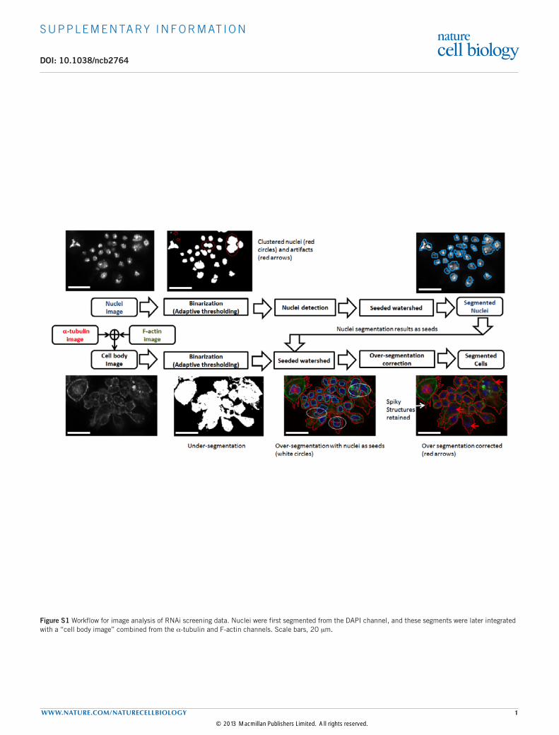
Figure S1 Yin

Figure S1 Workflow for image analysis of RNAi screening data. Nuclei were first segmented from the DAPI channel, and these segments were later integrated with a “cell body image” combined from the α-tubulin and F-actin channels. Scale bars, 20 mm.


http://www.nature.com/doifinder/10.1038/ncbxxxx


2 WWW.NATURE.COM/NATURECELLBIOLOGY

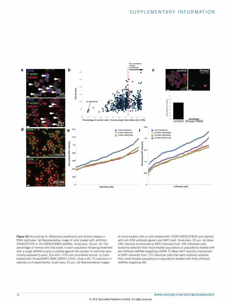
Figure S2 Accounting for differential penetrance and diverse shapes in RNAi replicates. (a) Representative image of cells treated with sti/Citron (DRSC09739) or Pvr (DRSC03080) dsRNAs. Scale bars, 20 mm. (b) The percentage of normal cells that exists in each population following treatment with a single dsRNA (x-axis) is plotted against the number of cells that were initially analysed (y-axis). ECs with >75% are considered normal. (c) Cells treated with thread/DIAP1 RNAi (DRSC11404), show a 96.7% reduction in viability (n=4 experiments). Scale bars, 20 mm. (d) Representative images

of mock-treated cells or cells treated with rl/ERK (DRSC07833) and stained with anti-ERK antibody (green) and DAPI (red). Scale bars, 20 mm. (e) Mean ERK intensity (normalized to DAPI intensity) from 195 individual cells randomly selected from mock-treated populations or populations treated with two different dsRNAs targetting rl/ERK. (f) Mean AKT intensity (normalized to DAPI intensity) from 170 individual cells that were randomly selected from mock-treated populations or populations treated with three different dsRNAs targetting Akt.

Cel

l Num

ber

Percentage of normal cells - N score larger than others ([L,C,T,R])

6000

0

5000

4000

3000

2000

1000

0.0 0.1 0.2 0.3 0.4 0.5 0.6 0.7 0.8 0.9 1.0

Pvr DRSC03080

stiDRSC09739

DNAF-actintubulin

DNAF-actintubulin

threadDRSC11404

control

0

0.2

0.4

0.6

0.8

1

1.2

1.4

control thread RNAi

Nor

mal

ised

cel

l num

ber

ERKDNA

ERKDNA

mock

rl/ERKDRSC07833

Nor

mal

ised

ER

K in

tens

ity

Individual cells

0.14

0.12

0.1

0.08

0.06

0.04

0.02

0

mock transfected

rl RNAi, DRSC07833rl RNAi, DRSC21814

Individual cells

Nor

mal

ised

AK

T in

tens

ity

f

0

0.05

0.1

0.15

0.2

0.25

mock transfected

Akt RNAi, DRSC30944Akt RNAi, DRSC36666

Akt RNAi, DRSC14108

d e

sti, DRSC09739

ECs considered normal(no filtering)

ca bFigure S2 Yin




Repeatability analysis

0

50

100

150

200

250

300

350

400

450 Repeatability analysis across dsRNAs

2 3 4 5 6 7

replicablenon-replicable

Number of dsRNAs targeting a single gene

Num

ber o

f dsR

NA

s

d

DRSC16650−DoaDRSC13893−DoaDRSC13892−DoaDRSC13896−DoaDRSC27825−PPP4R2rDRSC21503−PPP4R2rDRSC18695−PPP4R2rDRSC18695−PPP4R2r

1.2

1.4

1.6

1.8

2

1

0.8

0.6L C T R

−1

0

1

2

3

4

5

6

7

DRSC26851−sdtDRSC18108−sdtDRSC17861−sdtDRSC18022−sdtDRSC26053−Pp4−19CDRSC23319−Pp4−19CDRSC20559−Pp4−19CDRSC21251−Pp4−19CDRSC29546−dlg1DRSC18896−dlg1DRSC19767−dlg1DRSC20324−dlg1

L C T R

0

-0.5

0.5

1

1.5

2

DRSC23325−PTP−ERDRSC04636−PTP−ERDRSC28263−PTP−ERDRSC29144−rgDRSC17726−rgDRSC17726−rgDRSC23336−Gprk2DRSC16682−Gprk2DRSC16682−Gprk2

L C T R

00.5

1

1.52

-0.5-1

-1.5-2

DRSC29386−IrbpDRSC23317−IrbpDRSC17007−IrbpDRSC28430−mnbDRSC23347−mnbDRSC20353−mnbDRSC29095−Pi4KIIalphaDRSC12322−Pi4KIIalphaDRSC12323−Pi4KIIalpha

L C T R

b

−20

24

68

10

−4−3

−2−1

01

23−3

−2.5

−2

−1.5

−1

−0.5

0

0.5

1

1.5

2

L score

108 normal−like cells92 Pp2-14D cells with non-normal phenotypes200 Pp2-14D cells sampled after filtering

T score

R s

core

a

c

Figure S3 Yin

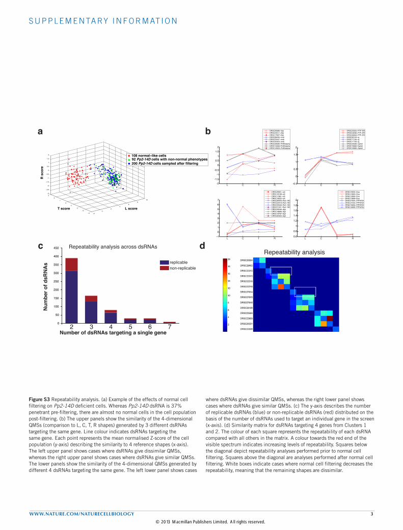
Figure S3 Repeatability analysis. (a) Example of the effects of normal cell filtering on Pp2-14D deficient cells. Whereas Pp2-14D dsRNA is 37% penetrant pre-filtering, there are almost no normal cells in the cell population post-filtering. (b) The upper panels show the similarity of the 4-dimensional QMSs (comparison to L, C, T, R shapes) generated by 3 different dsRNAs targeting the same gene. Line colour indicates dsRNAs targeting the same gene. Each point represents the mean normalised Z-score of the cell population (y-axis) describing the similarity to 4 reference shapes (x-axis). The left upper panel shows cases where dsRNAs give dissimilar QMSs, whereas the right upper panel shows cases where dsRNAs give similar QMSs. The lower panels show the similarity of the 4-dimensional QMSs generated by different 4 dsRNAs targeting the same gene. The left lower panel shows cases

where dsRNAs give dissimilar QMSs, whereas the right lower panel shows cases where dsRNAs give similar QMSs. (c) The y-axis describes the number of replicable dsRNAs (blue) or non-replicable dsRNAs (red) distributed on the basis of the number of dsRNAs used to target an individual gene in the screen (x-axis). (d) Similarity matrix for dsRNAs targeting 4 genes from Clusters 1 and 2. The colour of each square represents the repeatability of each dsRNA compared with all others in the matrix. A colour towards the red end of the visible spectrum indicates increasing levels of repeatability. Squares below the diagonal depict repeatability analyses performed prior to normal cell filtering. Squares above the diagonal are analyses performed after normal cell filtering. White boxes indicate cases where normal cell filtering decreases the repeatability, meaning that the remaining shapes are dissimilar.




Figure S4 Yin

a

b

4599 Non Tar (NT) 4599 PTEN RNAi #J05

4599 PTEN RNA i#J07 4599 PTEN RNAi #J08

A375p NT A375p PTEN RNAi#J09

A375p PTEN RNAi #J010 A375p PTEN RNAi #J011

NT #J05 #J07 #J08PTEN RNAi(s)

PTEN

Tot-AKT

pAKT

4599

NT

PTEN RNAi#J05

PTEN RNAi#J07

PTEN RNAi#J08

0

20

40

60p=0.0082

p=0.02 p=0.0099

% o

f Elon

gatio

nNT #J09 #J010#J011

PTEN RNAi

PTEN

Tot-AKT

pAKT

A375p

NT

PTEN RNAi#J09

PTEN RNAi#J01

0

PTEN RNAi#J01

10

20

40

60 p=0.0013 p=0.0028p=0.0017

% o

f Elon

gatio

n

Figure S4 PTEN depletion by RNAi leads to increased numbers of elongated cells. 4599.1 melanoma cells (a) and A375p melanoma cells (b) were transfected with non-targetting (NT) or PTEN RNAi(s) and seeded on a thick layer of Col-I. After 5-16 hrs of serum starvation, cells were photographed under phase contrast. Scale bars, 50 mm. Histograms show quantification

of the proportion of elongated cells (Mean±S.D.) in 4599.1 melanoma cells (a) and A375p melanoma cells (b) upon PTEN knockdown; 300 cells per n=3 experiments; Student’s t-test was used to generate p-value. Immuno-blots show the level PTEN and total (Tot) AKT in NT- and PTEN RNAi(s)-transfected 4599.1 (upper panel) and A375p (lower panel).




4599 NT 4599 shPTEN#J04 4599 shPTEN#J05

4599 (PTENwt) 690Cl2(PTENwt)

Figure S5 Yin

a

b

Figure S5 High magnification images of tumour sections following PTEN RNAi. Representative images of low magnification tumour sections derived from either non-targetting (NT), or PTEN shRNAs-expressing 4599.1 melanoma cells. Scale bars, 100 mm.




IRAK1

MARK2SLKSTK10PLK

MAPK1

MAPK3

YWHAZIR

AK1

MARK2SLKSTK10PLK

MAPK1

MAPK3

YWHAZ0

20

40

60

80

100Human (A375p)Mouse (4599)

% m

RN

A de

plet

ion

co-transfected

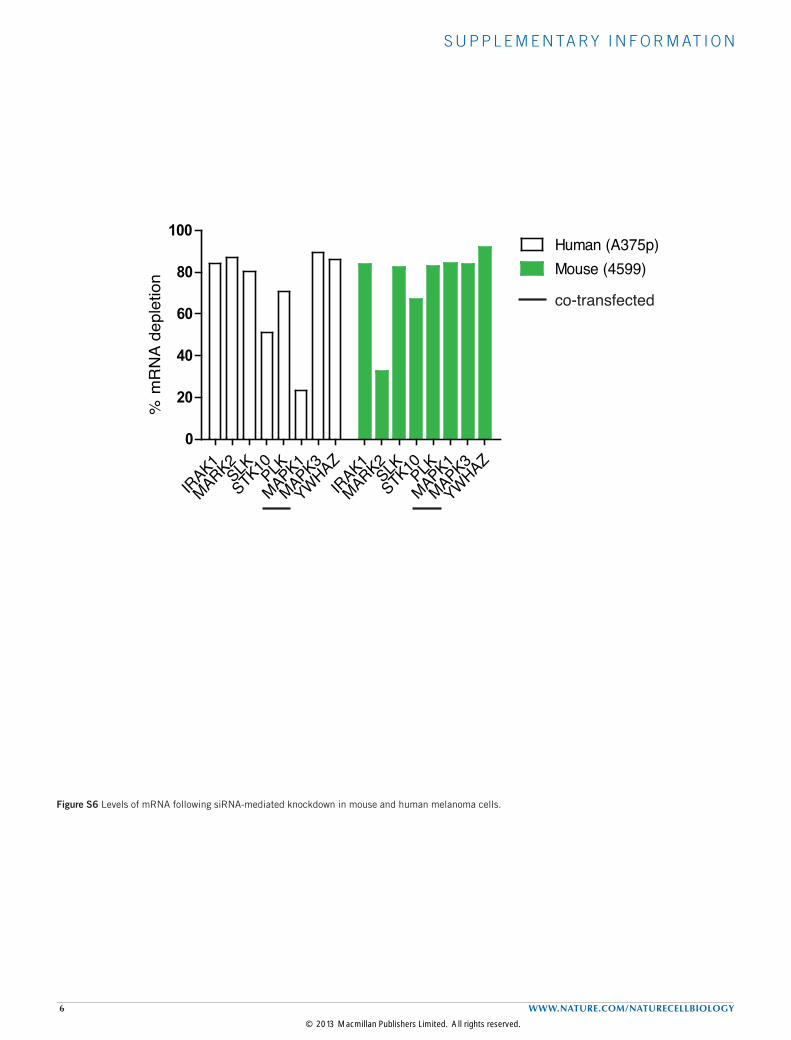
Figure S6 Yin

Figure S6 Levels of mRNA following siRNA-mediated knockdown in mouse and human melanoma cells.




52kDa

75kDa

N.T

52kDa

75kDa

J02 J04 J05.c

l3

J05.c

l4

52kDa

75kDa

N.T J02 J04 J05.c

l3

J05.c

l4

pAKT(Ser473)

Tot-AKT

PTEN

pAKT(Ser473)

Empty-E

GFP

EGFP-PTEN

52kDa

75kDa

52kDa

75kDa

PTENEmpty

-EGFP

EGFP-PTEN

Empty-E

GFP

EGFP-PTEN

52kDa

75kDa

Tot-AKT

Figure S7, Yin

Empty-E

GFP

EGFP-PTEN

150kDa

75kDa

Rock2

Relates to figure 7d


Relates to figure 7g





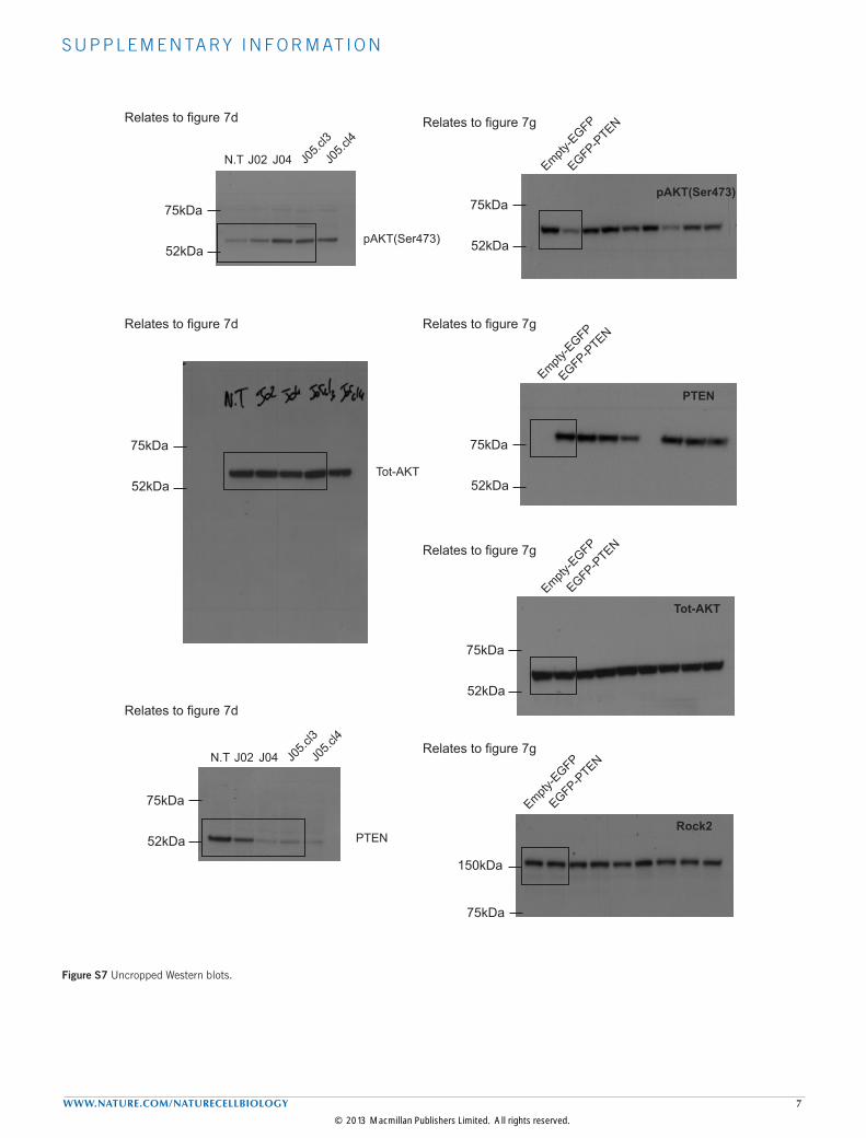
Figure S7 Uncropped Western blots.




Supplementary Table Legends

Table S1 Summary of whole-cell geometry features. Each one of 11 whole-cell geometry features is defined by a feature ID among the 211 morphology features. A brief description and the data source from where the specific feature is extracted.

Table S2 Summary of Haralick texture features extracted from the spatial-dependence matrix of each cell segment. The 14 Haralick features are divided into three groups, and the feature IDs among the 211 morphology features, as well as the feature names as defined in the original reference, are listed.

Table S3 Summary of regional geometric features. The 54 regional geometric features are divided into two groups, namely length ratios and area ratios. For each group, the feature IDs among the 211 morphology features are listed; a brief description for feature extraction are supplied; and an simple illustration for feature extraction process is shown.

Table S4 Summary of the four groups within the initial population of each GA run. The 200 individuals in each initial populations for a GA run is divided into four groups. Each group is defined based on the results of the previous SVM-RFE process, and the relationships between individuals in each group and the SVM-RFE results are defined.

Table S5 Quantitative Morphological Signature (QMS), Q(4), max RIFT, and mean RIFT scores for 287 ECs. In the first sheet we describe the number of repeatable cells that comprise each EC (column C), the number of cells from individual populations targetted by individual amplicons that contribute to total cell number. Each ECs QMS is comprised of L, T, C, and R scores and a PZ score. Cluster number is determined by hierarchical clustering (Fig. 3). In the second sheet the raw amplicon data for all tested amplicons is listed.

Table S6 Morphological comparison of PTEN wild-type and PTEN-deficient cells. Detail of data that is summarised in Fig. 7b.

Table S7 Drosophila genes chose for validation in mouse and human melanoma cells.

Table S8 Sequences for siRNAs and shRNAs used in mouse and human knockdown experiments.


Supplementary Note for

A Screen for Morphological Complexity Identifies Regulators of Switch-like Transitions between

Discrete Cell Shapes

*To whom correspondence should be addressed

E-mail: [email protected] (S.W.); [email protected] (C.B.); [email protected] (Z.Y.)


1

1. Image processing and cell morphology quantification We developed G-CELLIQ (Genomic CELLular Imaging Quantitator), an integrated workflow for

processing large volumes of digital images generated from high-throughput/genome-scale High-Content

Screens (HCS). G-CELLIQ is freely available for academic use [1]. Our software performs both image

segmentation and feature extraction as follows:

1.1 Image Segmentation

A three-stage cell segmentation method is used, consisting of nuclear segmentation, cell body

segmentation, and over-segmentation correction [2-5], as shown in Supplementary Fig. S1.

Nuclear segmentation: There are three steps in this stage: binarization, nuclei detection, and seeded-

watershed based nuclei segmentation [5, 6]. The binarization step features adaptive thresholding

technology: a data-driven background correction algorithm is first used to estimate the background with

cubic B-spline [7, 8]; each pixel is then classified as belonging to a nucleus or the background based on

the difference between its intensity and the estimated background intensity. Because binarization usually

fails to segment clustered nuclei [9], we applied further processing steps to binarization results to detect

nuclei. First a combined image is obtained as:

�� 0.8 ��;

��: the original image with intensity information; ��: the distance image obtained by applying the distance transform on the binary image [10].

�� is then filtered with a Gaussian filter (with standard deviation ). In the filtered image, the

noise is suppressed and the local maxima tend to correspond to the cell centers. Nuclei detection is then

carried out in the gradient vector field (GVF) to further eliminate the possible noisy local maxima[2, 11];

here, the redundant stains in the nuclei channel are removed by the non-maxima suppression operation.

Finally, given the nuclei centers defined from the combined image, marker-controlled seeded-

watershed methods are used to delineate the nuclei shapes.

Cell body segmentation: Cell body quantification needs information from both F-actin and α-tubulin

channels. The signal from these two channels are combined as � � �F�� . Adaptive

thresholding methods [7, 8] are used to separate the cell bodies from the background. After thresholding,

the nuclear segmentation results are planted onto the binary cell body image as the seed information, and

the seeded-watershed method [2] uses this seed information to delineate the cell bodies. This strategy

tackles the challenging cases where multiple cell bodies are touching each other.

Over-segmentation correction: Few cells are under-segmented due to the involvement of nuclei

information as seed for cell body segmentations. Conversely, an over-segmentation problem arises when

2σ =


2

there are multiple nuclear regions within cells (e.g. following failed cytokinesis). We implemented a

threshold based method to reduce the over-segmentation. Each cell segment is assigned a neighborhood

cell segment with which it shares the longest common boundary. Then a rectangular region is defined

across the common boundary of the two touching segmented patches, and the intensity variation within

the rectangle is calculated. The two patches are merged if intensity variation within the rectangle is

smaller than a given threshold.

Image quality control: The following procedure is implemented to select high quality cell images:

1) Before nuclei segmentation, the histogram and the calculated threshold for binarization for each

image are compared to those from manually validated good quality images to exclude extremely

dark or bright images.

2) Images with less than 10 candidate nuclei are discarded.

3) Cells that touch the image boundary are discarded.

1.2 Feature Extraction

To quantify the geometric and texture properties of each segmented cell, 211 morphology

features were extracted [3]. The selected features include a total of 85 wavelet features (70 features from

Gabor wavelet transformation [12] and 15 features from 3-level CDF97 wavelet transformation [13]), 11

whole-cell geometric features extracted from the whole cell body [3], 47 Zernike moments features with

a selected order of 12 [14], 14 Haralick texture features [15], and a total of 54 regional geometric

features extracted from divided parts of cell segments (36 features of ratio length of the central axis

projection and 18 features of area distribution over equal sectors) [3]. All features are extracted from

images generated by combining the three channels.

Wavelet features (feature No. 1~85): Two important types of discrete wavelet transformation, the

Gabor wavelet [12] and the Cohen–Daubechies–Feauveau wavelet (CDF9/7) [13], were applied to

extract cellular texture properties. We extracted the mean and standard deviation of Gabor texture

features, as defined in [16], with 6 scales and 4 orientations. Altogether, 70 features were obtained and

numbered 1~70 in the resulting feature set. Furthermore, 3-level CDF97 wavelet transformation [13]

was performed to extract additional texture signatures. In each level, the minimum, maximum, mean,

median of maximum distribution, and standard derivation were calculated for each transformed image.

In total, we obtained 15 CDF97 wavelet features from each cell segment, and included them as feature

No. 71~85.


3

Geometry-I: Whole-Cell Geometry features (feature No. 86~96):::: The 3-channel images for each cell

segment were first combined into a gray level image, then 11 geometry features were extracted using the

regionprops function in image processing toolbox of MatlabTM

, as defined in Supplementary Table S1.

Zernike moments features (feature No. 97~143): Based on [14], for each cell, Zernike moments of

order 12 were obtained within a unit circle centered at the cell mass center. Each order generated 4

features, and with the first output in the lowest order excluded, 47 moments features in total were

obtained.

Haralick texture features (feature No. 144~157): As a traditional texture signature, the Haralick Co-

occurrence features, with a total of 14 attributes listed in Supplementary Table S2, were extracted from

the gray-level spatial-dependence matrices for each cell segment [15].

Geometry II: Regional geometry features: Two groups of regional geometry features, “length ratios

of the central axis projection” and “the area ratio over equal sectors”, were extracted after further

dividing each cell segment, as summarized in Supplementary Table S3[3].

We define the cell centroid (mx, my) as the first order moments of the binary image f(x,y) for each

cell segment. A series of central radial axis are then defined as the line ��. The central projection along

�� is quantified by the length of the cell boundary contained by two neighboring central axes. The ratio

length of the central projection �� is defined as �� !" # $%�&�� where ' � # $%�&�()*+, -,++ � is

the perimeter of the cell, and 36 ratio length feature sets are evenly sampled around the cell.

The entire cellular region is partitioned into 18 sectors centered at the cellular centroid with even

radius angles; the ratio area is defined as the ratio between the area of the fan bin ./ to the area of entire

cell segment: �01 � # 2%3,5&�3�5%6,7&891# 2%3,5&�3�5 . The two shape descriptors are not invariant upon rotation of cell

segments, and we sorted the calculated ratio length and ratio area in descending order to partially

address this issue.

2. Phenotype modeling and cell classification

2.1 Feature selection using SVM-RFE and GA-SVM

To discriminate between different phenotypes (as judged by an expert), we need to identify a subset of

relevant features to these phenotypes from our 211 morphological phenotypes. Initially, SVM-RFE

(SVM-Recursive Feature Elimination) with linear kernel [17, 18] and cross validation was used to select

the top 20 informative features. However, it has long been argued that such "greedy combination" of

good individual features may not be the best option, and in most cases SVM-RFE tends to over-estimate


4

the optimal feature number. Thus, we performed a secondary feature selection using Genetic Algorithm

with SVM (GA-SVM) [19, 20]. Twenty initial populations, each having 200 individual features, were

created. Each initial population favors one of the top 20 candidate features from SVM-RFE, and each

population was divided into four groups, as detailed in Supplementary Table S4. GA optimizations were

run 20 times and selected the subset giving the lowest value of target function, which is the mean error

rate through 100 times 10-fold cross validations [17, 18] on the training dataset for each phenotype. In

both SVM-RFE and GA-SVM stages we used SVMs with linear kernel [21-23] to assess the criteria for

feature elimination and the fitness function for GA, respectively. SVMs were implemented using the

SVMTrain and SVMclassify functions of MatlabTM

.

The implementation of GA-SVM was based on the Genetic Algorithm and Direct Search

Toolbox in Matlab 7.1 (R14). Specifically, the option structure creation function gaoptimset used the

following parameters: population size of 200, maximum generation of 100, default crossover rate of 0.7

and mutation rate of 0.1. In each generation the top 3 elite individuals with the highest fitness function

were kept into the next generation.

2.2 Cell classification using SVM

A support vector machine (SVM) [21, 22] with Gaussian Radial Basis Function (RBF) kernel is used

for cell classification due to its flexibility to handle the non-linear relationships between the classes. For

each classifier, the continuous output from discriminate function f(x) is used directly to indicate the

similarity between the specific training set and test sample. Similar to [24], the classification result for

single cell is the basis of functional score for each experimental condition.

Grid search for SVM parameters: All SVMs involved were implemented using LIBSVM v3 package

[23]. An SVM with Gaussian RBF kernel has two main parameters: width for Gaussian kernel : and

penalty for training error C. A two-stage search of optimal parameters was applied. Using grid.py in [23],

the preliminary search employed exponentially growing sequences as ; 8 <2>|@ 8 Z, B8 C @ C 8Dand

: 8 <2E|F 8 Z, B12 C @ C 3D . For each combination of C and : , we carried out 10 times of 10-fold

cross validation on available training sets, and made sure that all samples were used as testing sample at

least once. The parameter set with the best cross-validation performance was selected as the candidate,

and a secondary search in linear scale was carried out in the neighborhood of the candidate to

determine the final parameter set for the corresponding SVM classifier.


5

3. Generation of Quantified Morphological Signature (QMS)

3.1 Morphological signature of each dsRNA

3.1.1 Quantifying single cell morphology using SVM classification results

SVM classifier attempts to find a hyperplane that best separates the positive and negative classes.

The raw output of SVM is the distance from x to the discriminant hyperplane and quantifies the

similarity between x and the given class. Thus, using five SVMs trained in 2.2, the morphology of each

single cell can be quantified by five scores. Specifically for each cell x, we have:

1) I3-+JKK , LMNII 8 <O, �, ;, P, QD, raw output from the SVM using class as the positive training set,

I3R comes from SVM using Normal cells as positive class; and similarly,

L denotes elongated, bipolar, spindle shaped cells;

C denotes very large flat cells with smooth edges;

T denotes small, partially polarized ‘teardrop’ shaped cells;

R denotes large flat ruffled cells

2) �3 � SI3R , I3� , I3T , I3U , I3VW, a 5-tuple score vector quantifying the cell morphology.

3.1.2 Normal cell filtering

We observe that different dsRNAs are variably penetrant in their effects on cell shape

(Supplementary Fig. S2). For example, a dsRNA targeting sticky results in a population where ~90% of

cells are large and bi-nucleate (Supplementary Fig. S2a), whereas a dsRNA that depletes Pvr results in

“L” cells in ~30% of the population (Supplementary Fig. S2a). By plotting the percentage of normal “N”

cells in each EC we could quantify penetrance (Supplementary Fig. S2b). Differential penetrance is not

due to differential uptake since dsRNAs targeting thread result in cell death in nearly 100% of cells

(Supplementary Fig. S2c).

In order to gain insight into the reasons for differential penetrance we used immunofluorescence

microscopy to quantify protein levels of Drosophila ERK and Akt in single cells where ERK and Akt

respectively were depleted by different dsRNAs (Supplementary Fig. S2d,e). Interestingly, we see that

protein levels of both ERK and AKT can vary by 2-3 fold in different wild-type populations, While

dsRNAs reduce these levels overall, there is still a population of cells with ERK or AKT levels that are

comparable to levels found in many wild-type cells. Thus we propose that differential penetrance is

largely due to the inability of different dsRNAs to knockdown protein levels below a certain threshold.

Mahalanobis distance [25] was used to determine whether a cell has similar morphology as the

predefined normal cell. Subsequently we could filter normal cells from different populations:


6

1) N=[�X], where each row vector �X quantify the morphology of a cell n, and cell n belongs to the

training set for Normal phenotype;

YZ, the mean vector for N;

ΣZ, the covariance matrix for N;

2) �3 � SI3R, I3� , I3T , I3U , I3VW for each single cell x;

3) [N%�3 , Z& � ]%�3 B YZ&ΣZ�!%�3 B YZ&T, the Mahalanobis distance between �3 and N;

4) M=S[N%�X , Z&W, all distances between the complete dataset N and each row vector �X within N;

Y_, the mean of M;

`_, the standard deviation of M.

The following criteria were used for normal cell filtering:

a) Given all cells within a single well, calculate [N%�3 , Z&;

b) Calculate the mean Pearson correlation coefficients between �3 and every score vector in N;

c) If �3 has i) [N%�3 , Z& a Y_ `_, ii) average correlation between �3 and N is larger than 0.85

and iii) I3R larger than any of <I3� , I3T , I3U , I3VD, the corresponding cell x is considered a normal cell.

d) If less than 75% cells are considered normal in a well, remove the normal cells based on step c).

The threshold of 75% is set according to the mean (0.8872) and standard deviation (0.1129) for

the ratio of normal cells across all wells in control baseline (Supplementary Fig. S2b).

3.1.3 Raw morphology score for a single well

Given a single well w, after image quality control and normal cell filtering, the raw morphology

score Sw is the average of single cell scores in w.

3.1.4 Normalization of raw well scores

899 dsRNAs were deployed into 5 different plates. Each deployment was repeated 3 times, thus any

given dsRNA was repeated at least three times. Two types of negative control wells exist in each plate:

“control empty” wells where no dsRNA was added and “control LacZ” wells where a null dsRNA

targeting LacZ was added and was not supposed to cause any phenotype change. We have:

Control baseline b � S�cW, all raw morphology scores of more than 200,000 cells belonging to

control wells;

db � SdeR , de� , deT , deU , deV W , the mean of B;

`b � SèR, è� , èT , èU , èVW the standard deviation of B;


7

Thus, given any raw score vector fg � SIgR , Ig� , IgT , IgU , IgVW for certain well w, we normalize Sw into the

Z-score of control baseline, i.e. hg-+JKK � Kgijkll�mnijkllonijkll , LMNII 8 <O, �, ;, P, QD . The normalized score

pg � Shg-+JKK, hg-+JKK, hg-+JKK, hg-+JKK, hg-+JKKW quantifies the morphological change in well w comparing to

control baseline.

3.1.5 Repeatability test for wells using a same dsRNA

To test for repeatability, we test whether wells that are treated with dsRNA D form a compact cluster,

i.e. whether cells treated with D have a significantly smaller dispersion than random group of cells. We

denote wells with the same dsRNA D by WD={w1,…wn}:

1) the dispersion measurement qrs � tuv% wxy ∑ { |}~� , }~��x�,�8rs & , where denotes the

Mahalanobis distance between two vectors;

2) 1000 randomly sampled cell groups rs%E& � <g!%�&, … gy%�&D, F � 1,2 … 1000. Each rs%E& has the

same number of wells as WD, and each well g�%�&, � � w, x … y consists of cells from the same

plate as wi ; i.e. each rs%E& has the same cell number as WD, while containing cells randomly

sampled from the plates containing wells w1,…wn ; and thus the random sampled cells are

subject to non-specific RNAi treatments;

3) 1000 random dispersion measurements qrs%�& , � � w, x … w��;

4) qs� , the mean value of qrs%�&, � � w, x … w��, and �s�, the estimated distribution of qrs%�& from

the non-parameterized Parzen window method [26].

A one tail permutation test is set up with �s� as the null distribution:

Null hypothesis H0: qrs � qs� ;

i.e. qrs (dispersion for cells with a same dsRNA) is from the same distribution �s� as the cells subject

to random RNAi.

Alternative hypothesis H1: qrs C qs� ;

i.e. when targeted by a same dsRNA, the cells show a significantly smaller dispersion than the cells

undergoing random RNAi.

The null hypothesis is rejected at 5% significant level and is carried out in an iterative manner, such

that when null hypothesis cannot be rejected for WD={w1,…wn}, the tests are repeated while members

in WD are iteratively removed, until:

Either null hypothesis is rejected for a subset of WD , whose size is no smaller than n/2;

Or all subsets are deemed unrepeatable.

( , )d • •


8

Due to the facts that a) cells for a real well wi and a permuted well g�%�& come from the same plate; b)

each plate has different standard deviation on cellular morphology scores; and c) wells treated by a

certain dsRNA can be located in a same or different plates, and each plate is repeated several times, the

statistical power of this test varies when different plates are involved. When Parzen window estimation

is used, 1000 permutations is always enough to detect effect size of 1.5 with 0.85 power at 5% false

discovery rate (FDR).

3.1.6 Consolidation of scores through weighted average

Assume the permutation test in 3.1.5 identified a group of repeatable wells for dsRNA D, the

consolidated morphology signature for D is obtained, where the reciprocal of the Mahalanobis distance

from one well to general control baseline serve as the weight for each well, specifically we have:

1) nD , the size for the repeatable group identified in 3.1.5;

2) Zw, the normalized morphology score for a (repeatable) well w from 3.1.4;

3) dw, Mahalanobis distance from a (repeatable) well w to control baseline;

The consolidated score for dsRNA D has the form of: p� � %∑ w{g� fg�y��w & %∑ w{g�&y��w� .

3.2 Morphological signature of each gene

Even after filtering (Supplementary Fig. S3a) different dsRNAs targeting a same gene can elicit

very different responses (Supplementary Fig. S3b,c), similar to 3.1.5, repeatability tests were also

carried out on all dsRNAs targeting a same gene.

3.2.1 Repeatability test based on Mahalanobis distance

A permutation test similar as in 3.1.5 was applied. Assume dsRNAs D1 and D2 are biological

replicates targeting a same gene G, we have:

1) p�w and p�x , the morphological signature for D1 and D2, respectively;

2) {�}�w , }�x�, the Mahalanobis distance between two signatures;

3) 1000 randomly sampled cell groups �%E& � <�!%�& , �x%�&D, F � 1,2 … 1000. Each sampled cell

group ��%�& % � � w, x; � � w, x … w��& has the same number of wells as real cell group Di,

and each sampled well in ��%�&consists of cells from the same plate as the corresponding real

well in Di ; i.e. each ��%�& has the same cell number as Di, while containing cells randomly

sampled from the plates containing corresponding real wells and thus the random sampled

cells are subject to non-specific RNAi treatments;

4) 1000 random Mahalanobis distances {%�!%�&, �x%�&&, � � w, x … w��;


9

5) d0, the mean value for {%�!%�&, �x%�&&, � � w, x … w��; and P0, the estimated distribution of

{%�!%�&, �x%�&& from the non-parameterized Parzen window method [26].

A one tail permutation test is set up with P0 as the null distribution:

Null hypothesis H0: {�}�w , }�x� � {�;

i.e. {�}�w , }�x� (Distance for cells with a dsRNAs targeting a same gene) is from the same distribution

P0 as the cells subject to random RNAi;

Alternative hypothesis H1: {�}�w , }�x� C {�;

i.e. When subject to dsRNAs targeting a same gene, the morphology signatures show a significantly

smaller distance than those from cells undergoing random RNAi.

The null hypothesis is rejected at 5% significant level, and unlike 3.1.5, no iterative steps are

necessary because we directly work on each pair of dsRNAs. Also for each pair of dsRNAs, two p-

values are calculated based on the cell populations before- and after normal cell filtering, respectively.

Due to the facts that a) cells for a real well wi and a permuted well g�%�& come from a same plate;

b) each plate has different standard deviation on cellular morphology scores; and c) wells treated by a

certain dsRNA can be located in a same or different plates and each plate is repeated several times, the

statistical power of this test varies when different plates are involved. When Parzen window estimation

is used, 1000 permutations are always enough to detect effect size of 1.5 with 0.86 power at 5% false

discovery rate (FDR).

3.2.2 Repeatability test based on kernel density estimation and KL/J divergence

The test in 3.2.1 works on the average scores ZD across cell populations. Next, we consider the

heterogeneity within each cell population and set up a test on the similarity between two probability

distributions estimated from the score matrices of two cell populations.

General Denotation: Assume that a cell population D contains n single cells, and the morphology of

each cell x can be depicted by a 5-tuple score vector, which is normalized to Z-score of control baseline

and denoted as �3 � Sh3R, h3�, h3T , h3U , h3VW. Thus, based on the scoring profile p � S��W, � � 1,2 … � for D, a

distribution can be estimated for any LMNII 8 <O, �, ;, P, QD using the non-parameterized Parzen window

method [26]. Basically, a Gaussian kernel was applied around each single score h�-+JKKas ��ijkll��ijkllℎ

� �!√�� exp SB !� %�ijkll��ijkll

ℎ&�W , and the estimated probability distribution function (PDF) for any single

score from population D is denoted as: �%h�-+JKK& � !Xℎ∑ � ��ijkll��ijkllℎ

�X��! . Where h is a smooth


10

parameter referred to as bandwidth, and an acceptable guess is ℎ � 1.06`n��.�, where ` denotes the

standard deviation of h�-+JKK in � [27].

Bandwidth Estimation: Here we use a point-wise strategy from [27] to adjust bandwidth in the

distribution estimation. Given p � S��W, � � 1,2 … � for cell population D, hierarchical clustering was

carried out based on average linkage, unbiased Pearson correlation coefficients (PCC) between the 5-

tuple vectors I� were calculated, and those cells with PCC greater than 0.9 were assigned into a same

subgroup. Thus, G different subgroups g=1, 2…G can be defined, and we use ng to denote the number

of cells in each subgroup g. A fast one-dimensional Newton optimization was used to minimize the

leave-one-out cost function � -+JKK%ℎ& � B ∑ M¡¢� ��-+JKK%h�-+JKK,ℎ&X£��! , in search of local bandwidth

ℎ -+JKK for each g. Finally, the estimated distribution of score f can be re-organized based on the afore-

mentioned cell sub-group assignments as �%h�-+JKK& � !X ∑ ∑ !ℎ£ � ��ijkll��£,�ijkll

ℎ£ �X£��!¤ �! .

K-L divergence and J-divergence: After estimating a PDF for each score vector for each cell

population, we use the J-divergence to measure the difference between two such PDFs. The Kullback–

Leibler divergence [28] is a non-symmetric measure of the difference between two probability

distributions P and Q, as KL%P||Q& � # P%©&log P%3&Q%3& d©. Further, J-divergence is developed to make it a

symmetric metric in J%P||Q& � %KL%P||Q& KL%Q||P&&/2 [29, 30].

Permutation test for repeatability: Given two cell populations D1 and D2, the distributions of five

morphological scores are available as ��h��-+JKK�, LMNII 8 <O, �, ;, P, QD, � � 1,2 . To avoid the

computational burden in the following steps, we assume mutual independence among all scores. Thus,

the overall difference between morphological profiles for D1 and D2 can be defined as J%�w |�x& �∑ ²%��h�w-+JKK�||��h�x-+JKK�&, LMNII 8 <O, �, ;, P, QD . Let D1 and D2 denote cell populations generated by

two dsRNAs targeting the same gene, similar to 3.2.1., we have:

1) J%�w |�x&.

2) 1000 randomly sampled cell groups �%E& � <�!%�& , �x%�&D, F � 1,2 … 1000. The rule of cell

sampling is the same as in 3.2.1;

3) 1000 random divergences J|�!%�& ³�x%�&�, � � w, x … w��;

4) J0, the mean value for J|�!%�& ³�x%�&�, � � w, x … w��, and P0, the estimated distribution of

J|�!%�& ³�x%�&� from the non-parameterized Parzen window method [26].

A one tail permutation test is set up with P0 as the null distribution:


11

Null hypothesis H0: J%�w |�x& � ²�;

i.e. J%�w |�x& (divergence for cells with dsRNAs targeting the same gene) is from the same distribution

P0 as the cells subject to random RNAi;

Alternative hypothesis H1: J%�w |�x& C ²�;

i.e. when subject to dsRNAs targeting the same gene, the morphology signatures show a significantly

smaller distance than those from cells undergoing random RNAi.

The null hypothesis is rejected at 5% significant level, and for each pair of dsRNAs, two p-values are

calculated based on the cell populations before and after normal cell filtering, respectively. The

statistical power of this test varies when different plates are involved. However, when Parzen window

estimation is used, 1000 permutations is always enough to detect effect size of 1.5 with 0.90 power at 5%

false discovery rate (FDR).

3.2.3 Generation of QMS (Quantitative Morphological Signature) for each gene

Phenotypic scores: Similar to 3.1.6, the consolidated score for a single gene G has the form: p¤ �%∑ w{�� pg�y¤��w & %∑ w{��&y¤��w� . Where ZG denotes the consolidated score for a gene, dD is the Mahalanobis

distance from the morphology signature of a repeatable dsRNA to the signature of control baseline, and

nG

is the number of repeatable dsRNAs for gene G.

Penetrance Z-score: All cell populations underwent normal cell filtering, and those non-normal cells

were considered to be a result of the specific RNAi treatment – or “penetrant”. For each gene, we

summed the number of penetrant cells in all repeatable wells, and determined the ratio of penetrant cells,

which was then normalized based on the mean and standard deviation of penetrant cell ratio for control

baseline wells to get a penetrance Z-score, denoted as PZ.

Finally, for each gene G, four phenotype scores were combined with PZ to form a 5-tuple QMS

Spµ́ , p¶́, p·́, p´̧ , p¹́}W.

4. Analysis of QMSs

4.1 Hierarchical clustering

In our case, 899 dsRNAs were initially used to inhibit and the majority of known predicted kinases and

phosphatases and several kinase/phosphatase regulatory subunits and adapters (KP set) in Kc167 cells.

116 of these showed poor technical repeatability, 71 show poor biological repeatability, and 155 were

excluded from the final analysis as no repeat was performed. Thus, the scores from 557 dsRNAs were

used in generating the QMSs used in hierarchical clustering (Fig. 3 and Supplementary S5) or to


12

calculate the divergence matrix (Fig. 4c of the main text). We also calculated QMS for two types of

negative controls separately and incorporated them into the QMS matrix, thus generating 284

genes/conditions for hierarchical clustering. Hierarchical clustering using average linkage was

performed with Cluster [31] and JavaTM

TreeView [32] using uncentered Pearson Correlation

Coefficients as the similarity metric; clusters were defined interactively by finding the highest nodes at

which the distance measure became greater than 0.90. Other similarity thresholds were evaluated and

this was chosen because this level of correlation resulted in coherent groups of qualitatively similar cells.

Enrichment test reveal biological relevance for resulting phenoclusters: Hierarchical clustering of

284 ECs obtained 14 phenoclusters, including 4 singular genes and 10 phenoclusters with at least two

members. Fisher's exact tests were applied to identify the enrichment of biological themes, including

pathways, GO terms, and other function annotation terms, using the Database for Annotation,

Visualization and Integrated Discovery (DAVID) v6.7 [33]. As input for DAVID, all gene symbols

involved in hierarchical clustering were converted into Entrez ID using the Gene ID conversion tool in

DAVID and the Gene and reagent lookup tool from Drosophila RNAi screening center [34]. For each

obtained p-value from Fisher's test, Benjamini corrected p-value and False Discovery Rate were

calculated to address for multiple tests.

4.2 Using divergence scores to address cellular heterogeneity

Cell-to-cell differences are always present to some degree in any cell population, thus the mean

score of a population may not represent the behaviors of any individual cell [35]. Here, we propose to

use divergence based scores to address the heterogeneity of phenotypic cell populations.

General Denotations: Here, the kernel density estimation and divergence calculation methods in 3.2.2

are extended to the gene level. Assuming each cell population D includes all n cells, and the same local

bandwidth estimation has been carried out. The distribution of each feature LMNII 8 <O, �, ;, P, QD for

population D can thus be modeled by �%h�-+JKK& � !X ∑ ∑ !ℎ£,� � ��ijkll��£,�ijkll

ℎ£,� �X£��!¤ �! . Using the symmetric

divergence metric J between two distributions, the overall difference between two populations D1 and

D2 can be obtained. Thus we had J�,º � J�� »��, �, ¼ 8 <1,2 … 284D, � ¾ ¼ for all 284 ECs. Meanwhile,

J�,� were assigned the ceiling value of the maximum J�,º , � ¾ ¼ . Each divergence score was then

normalized into a similarity measurement by Q�,º � %max%J& B J�,º&/%max%J& B min %J�,º&. Larger values

of Q�,º indicate better similarity in phenotype composition (both morphology and ratio) between genes i

and j, and the genes in the same phenocluster should have relatively high value amongst each other.

The matrix Q is visualized as in Fig. 3c of the main text.


13

Quantifying the differentially sized shape space explored by cell populations: Based on Q�,º, we

defined a score Q(4)i, i=1,2…284 for the analysis of gene-level cell populations. Given the matrix Q in

the previous section, for each gene i, Q(4)i=Q(2)i-Q(1)i the difference between the mean population

similarity calculated on all genes other than i, (Q(1)i ) and all genes within the same cluster as gene i

(Q(2)i). Meanwhile, Q(3)i is gene i’s mean population similarity with all genes not in the same cluster as

i. In an ideal case, large Q(4)i indicates that RNAi treatment of gene i results in cells exploring a unique

area in phenotypic space, and the cell populations are only similar to those in the same phenocluster.

When this value is larger than the mean value of the wild-type cells (0.159), the difference is greater

than 1 standard deviation (S.D.) of genes in wild-type clusters, and the mean QMS of the population is

also different than wild-type cells, these populations are exploring regions of morphological space that

are both smaller and distinct from the space explored by the control populations. When this value is

smaller than the wild-type mean by a difference greater than 1 standard deviation, the population is

considered to be exploring a larger region of space than wild-type cells.

5. Network analysis for screening hits in human

5.1 Extraction of a Protein-Protein Interaction (PPI) network in human

Human PPI networks were obtained from STRING database [36] v9.0, and only those interactions with

confidence score larger than 0.6 were used. As a result, 604,897 PPI entries involving 16,518 proteins

were selected. Here PPIs were recorded in a directed pattern; thus, a common physical interaction

between proteins A and B was recorded as two entries A->B and B->A. Meanwhile certain “directed”

interaction categories like gene fusion or transcription factor binding only had one entry. According to

the graphconncomp function from MatlabTM

, 16,452 out of these 16,518 proteins form a strongly

connected component, meaning that given the 604,897 PPI entries, and any two proteins A and B in this

component:

1) A and B can be connected by selected PPI entries;

2) Both paths A->B and B->A are available without violating the direction of each involved entry.

3) The lengths of shortest paths A->B and B->A are given by graphallshortestpaths function in

MatlabTM

.

5.2 Functional Roles of human homologs for genes with high L scores

Three groups of proteins (Fig. 7d of the main text) were mapped into the connected human PPI network

from 5.1:

1) Group-1– 14 proteins have been previously defined as “pro-elongation” proteins, and include:


14

CrkL, DOCK3, Integrin beta 1, LIMK2, p27Kip1, p53, p130Cas, NEDD9, MyoP, Rab5, RhoE,

SMURF2, Src, WASF2;

2) Group-2– 12 proteins have been previously defined as “pro-contractility” proteins, and include:

3) DIP1, EphrinA, FHOD2, gp130, IL-6, LIMK1, MYL2, PAK2, PDK1, RhoC, STAT3, Stathmin1;

4) Group-3– 15 proteins, whose inhibition results in elongation in mouse or human cells (Fig. 7)

and include:

PLK1, 14-3-3zeta, PTEN, IRAK1, JAK1, PAR-1, MAPK3, MAPK1, SLK, LOK, Cdk4, Cdk10,

MAST1/2, Liprin-B2.

The lengths of shortest paths among any two out of these proteins was obtained in 5.1. Specifically,

for each protein p in group-3 and any protein x from the connected component with 16,452 members,

we have:

a) L(p, g1), the mean of shortest-path-lengths between protein p and every member in Group-1;

b) {L(x, g1)}, the array of mean shortest-path-lengths between any protein x and every member in

Group-1;

Lg1, the mean of {L(x, g1)};

̀!, the standard deviation of {L(x, g1)};

c) Z(p, g1)=[L(p, g1)- Lg1]/ ̀!;

d) L(p, g2) and Z(p, g2), defined similarly between protein p and group-2;

e) Diff(p, g1, g2)=L(p, g1)- L(p, g2), p belongs to group-3;

Diff(x, g1, g2)=L(x, g1)- L(x, g2), x is any one of the 16,452 connected proteins;

Z-scores Z(p, g1) and Z(p, g2) indicate whether p is closer/further from group-1 or -2 compared to

random proteins in the connected component, with a Z-score smaller than -1.98 translating to a p-value

<0.05 in standard normal distribution. Meanwhile, Diff(p, g1, g2) quantifies whether p is closer to group

A or group B. It is worth noting that the mean of Diff(x, g1, g2) across 16,452 proteins is -0.08, thus a

random protein tends to be closer to group-1 than group-2. However, our group-3 can be divided into 3

subsets:

i) Diff(p, g1, g2)>1, closer to Group-2 and projected as positive regulator of Group-2;

ii) Diff(p, g1, g2) between [-0.08, 1];

iii) Diff(p, g1, g2)<-0.08, closer to Group-1 and projected as negative regulator of Group-1.

References

1. http://www.cbi-tmhs.org/GCellIQ/NCB. [cited.


15

2. Li, F.H., X. Zhou, and S.T.C. Wong, An automated feedback system with the hybrid model of

scoring and classification for solving over-segmentation problems in RNAi high content

screening. Journal of Microscopy, 2007. 226(2): p. 121 - 132.

3. Wang, J., et al., Cellular Phenotype Recognition for High-Content RNA Interference Genome-

Wide Screening. Journal of Molecular Screening, 2008. 13(1): p. 29-39.

4. Xiong, G., et al., Automated segmentation of Drosophila RNAi fluorescence cellular images

using deformable models. IEEE Transactions on Circuit and Sysrems, 2006. 53: p. 2415 - 2424.

5. Yan, P., et al., Automatic segmentation of RNAi fluorescent cellular images with interaction

model. IEEE Transactions on Information Technology in Biomedicine, 2008. 12(1): p. 109 - 117.

6. Li, F.H., et al., High content image analysis for human H4 neuroglioma cells exposed to CuO

nanoparticles. BMC Biotechnology, 2007. 7: p. 66.

7. Lindblad, J., et al., Image analysis for automatic segmentation of cytoplasms and classification

of Rac1 activation. Cytometry A, 2004. 57(1): p. 22-33.

8. Wahlby, C., et al., Algorithms for cytoplasm segmentation of fluorescence labelled cells.

Analytical Cellular Pathology, 2002. 24(2-3): p. 101-11.

9. Vincent, L. and P. Soille, Watersheds in digital spaces: an efficient algorithm based on

immersion simulations. IEEE Transactions on Pattern Analysis and Machine Intelligence, 1991.

13(6): p. 583-598.

10. Borgefors, G., Distance transformations in digital images. Computer Vision, Graphics, and

Image Processing, 1986. 34: p. 344-371.

11. Wang, M., et al., Novel cell segmentation and online SVM for cell cycle phase identification in

automated microscopy. Bioinformatics, 2008. 24(1): p. 94-101.

12. Manjunatha, B.S. and W.Y. Ma, Texture features for browsing and retrieval of image data. IEEE

Transactions on Pattern Analysis and Machine Intelligenece, 1996. 18: p. 837 - 842.

13. Cohen, A., I. Daubechies, and J.C. Feauveau, Bi-orthogonal bases of compactly supported

wavelets. Communications on Pure and Applied Mathematics, 1992. 45: p. 485 - 560.

14. Zernike, F., Beugungstheorie des schneidencerfarhens undseiner verbesserten form, der

phasenkontrastmethode. Physica, 1934. 1: p. 689 - 704.

15. Haralick, R.M., K. Shanmugam, and I. Dinstein, Textural features for image classification. IEEE

Transactions on Systems, Man and Cybernetics, 1973. 6: p. 610 - 620.

16. Daugman, J.G., Complete discrete 2-D Gabor transforms by neural networks for image analysis

and compression. Acoustics, Speech and Signal Processing, IEEE Transactions on, 1988. 36(7):

p. 1169-1179.

17. Guyon, I., et al., Gene Selection for Cancer Classification using Support Vector Machines.

Machine Learning, 2002. 46(1-3): p. 389-422.

18. Li, G.Z., et al. Feature selection for multi-class problems using support vector machines. 2004:

Springer-Verlag Berlin.

19. Holland, J., Adaption in Natural and Artifical Systems. 1975, Ann Arbor, MI: The University of

Michigan Press.

20. Goldberg, D., Genetic Algorithms in Search, Optimization and Machine Learning. 1989, Boston,

MA: Kluwer Academic Publishers.

21. Vapnik, V., The Nature of Statistical Learning Theory. 1995: New York, NY: Springer-Verlag.

22. Cortes, C. and V. Vapnik, Support-vector network. Machine Learning, 1995. 20: p. 273-297.

23. Chang, C.-C. and C.-J. Lin, LIBSVM: a library for support vector machines. 2001. p. Software

available at http://csie.ntu.edu.tw/cjlin/libsvm.

24. Bakal, C., et al., Quantitative morphological signatures define local signaling networks

regulating cell morphology. Science, 2007. 316: p. 1753 - 1756.

25. Mahalanobis, P.C., On the generalized distance in statistics. Proceedings of the National

Institute of Science of India, 1936. 2(1): p. 49-55.


16

26. Parzen, E., On estimation of a probability density function and mode. The Annals of

Mathematics Statistics 1962. 33: p. 1065-1076.

27. Scott, D. and S. Sain, Multi-dimensional density estimation. Handbook of Statistics, 2004. 24.

28. Kullback, S. and R.A. Leibler, On information and sufficiency. The Annals of Mathematics

Statistics, 1951. 22: p. 76-86.

29. Lin, J., Divergence measures based on the Shannon entropy. Information Theory, IEEE

Transactions on, 1991. 37(1): p. 145-151.

30. Johnson, D. and S. Sinanovic, Symmetrizing the Kullback-leibler Distance. 2001, Rice

University.

31. de Hoon, M.J.L., et al., Open source clustering software. 2004. p. 1453-1454.

32. Saldanha, A.J., Java Treeview--extensible visualization of microarray data. 2004. p. 3246-3248.

33. Huang, D.W., B.T. Sherman, and R.A. Lempicki, Systematic and integrative analysis of large

gene lists using DAVID bioinformatics resources. Nat. Protocols, 2008. 4(1): p. 44-57.

34. http://www.flyrnai.org/cgi-bin/DRSC_gene_lookup.pl. [cited.

35. Altschuler, S.J. and L.F. Wu, Cellular Heterogeneity: Do Differences Make a Difference? Cell,

2010. 141(4): p. 559-563.

36. Jensen, L.J., et al., STRING 8-a global view on proteins and their functional interactions in 630

organisms. Nucleic Acids Research, 2009. 37(suppl 1): p. D412-D416.


Documents

A screen for morphological complexity identifies