Embed Size (px)
Citation preview
STATISTICS IN MEDICINEStatist. Med. 2003; 22:3115–3132 (DOI: 10.1002/sim.1542)
A score test for binary data with patient non-compliance
Michael Branson1;2;∗;† and John Whitehead2
1Novartis Pharma AG; Lichtstrasse 35; CH-4056; Basel; Switzerland2Medical and Pharmaceutical Statistics Research Unit; The University of Reading; P.O. Box 240; Earley Gate;
Reading; RG6 6FN; U.K.
SUMMARY
A score test is developed for binary clinical trial data, which incorporates patient non-compliance whilerespecting randomization. It is assumed in this paper that compliance is ‘all-or-nothing’, in the sensethat a patient either accepts all of the treatment assigned as speci�ed in the protocol, or none of it.Direct analytic comparisons of the adjusted test statistic for both the score test and the likelihood ratiotest are made with the corresponding test statistics that adhere to the intention-to-treat principle. It isshown that no gain in power is possible over the intention-to-treat analysis, by adjusting for patientnon-compliance. Sample size formulae are derived and simulation studies are used to demonstrate thatthe sample size approximation holds. Copyright ? 2003 John Wiley & Sons, Ltd.
KEY WORDS: non-compliance; binary data; score test; likelihood ratio test; Wald’s test; sample size
1. INTRODUCTION
Ideally in medical research, once a patient has been randomized to a treatment, they willcomply fully with their treatment. However, in some areas of medical research, patient non-compliance is sometimes intentional or unavoidable, for example it may be desirable to runa prospective randomized controlled parallel group clinical trial but ethically not possible.Many trials in AIDS and various cancers have been reported in which patients have eitherbeen permitted to ‘switch’ treatment or have simply started to take alternative medication(s)whilst in the clinical trial. The motivation for allowing patients to switch treatment varies fromtrial to trial, but includes (i) the ethical concern that denying a patient a potentially bettertreatment is inappropriate and (ii) the realization that without allowing patients the option toswitch treatment, patient recruitment may be extremely di�cult.Correcting for patient non-compliance has been the focus of an increasing number of authors
who have devised analytical approaches aimed at uncovering the e�ects of ‘non-randomized’
∗Correspondence to: Michael Branson, Novartis Pharma AG, Lichtstrasse 35, CH-4056, Basel, Switzerland†E-mail: [email protected]
Contract=grant sponsor: MRC; contract=grant number: G78=5359
Received November 2001Copyright ? 2003 John Wiley & Sons, Ltd. Accepted March 2003
3116 M. BRANSON AND J. WHITEHEAD
treatment on patient outcome. Indeed, an entire edition of Statistics in Medicine [1] wasdedicated to the discussion of ‘Analysing non-compliance data in clinical trials’. For survivaldata, Robins and co-workers [2–7] have developed approaches for estimating the ‘causale�ect of treatment’ – in the sense of Rubin’s causal model [8, 9]. These approaches havebeen extensively applied by White et al. [10–12] to unravel the in�uence of non-randomizedtreatment on patient outcome. An estimation algorithm that builds on the ideas of Robins andTsiatis [2] was discussed by Branson and Whitehead [13]. Baker [14] has also investigatedthe analysis of survival data with ‘all-or-nothing’ compliance information.For binary outcome data, Sommer and Zeger [15] developed a statistical model that was
then generalized by Cuzick et al. [16] to allow for a scenario involving more complex ‘allor-nothing’ non-compliance information. Sato [17, 18] has investigated the use of complianceinformation, for binary data, based on the approach of Mark and Robins [6]. Goetghebeuret al. [19] developed a statistical model for ordinal response data that is also applicableto grouped survival data. In a recent article, Frangakis and Rubin [20] discuss patient non-compliance using a general ‘missing data’ model. In this paper we recommend that analyseswhich adjust for patient non-compliance are used to supplement rather than to replace thoseadhering to the intention-to-treat principle.We focus on data arising from randomized clinical trials in which patients are permitted
to change their administered treatment. For each patient it is assumed that their responsemay be classi�ed as a dichotomous outcome. It is assumed in this paper that complianceis ‘all-or-nothing’, in the sense that a patient either accepts all of the treatment assigned asspeci�ed in the protocol, or none of it. A score test statistic is developed for the modelproposed by Cuzick et al. [16], and its application is illustrated by an analysis of data from aBritish Medical Research Council (MRC) clinical trial (LU17) in non-small-cell lung cancer(NSCLC) [21].In Section 2, we discuss and summarize the data from LU17. The probability model of
Cuzick et al. [16] is presented in Section 3. Statistical inference based on the likelihood ratiotest, the score test and, for comparison purposes, Wald’s test, is discussed in Section 4. InSection 5, we derive formulae to perform sample size calculations and in Section 6 simulationis used to evaluate the error rates (type I and type II) for the score test statistic comparedwith those for Wald’s test statistic. The analysis of the data from LU17 is given in Section 7and concluding remarks are given in Section 8.
2. MOTIVATION: A CLINICAL TRIAL IN NON-SMALL-CELL LUNGCANCER (LU17)
This clinical trial was designed to compare immediate to delayed thoracic radiotherapy inpatients with non-small-cell lung cancer (NSCLC). Patients were randomized either to im-mediate radiotherapy or to ‘standard patient care’ until radiotherapy was advocated: we willdenote these two arms by E and C, respectively. Prior to LU17 being run, there existed di�er-ing opinions about the bene�t of immediate radiotherapy, although available publications werebased primarily on non-randomized trial data. At the design stage of trial LU17, immediateradiotherapy was advocated by Phillips and Miller [22] and Cox et al. [23] while Brashear[24] and Cohen [25] suggested that a ‘delay’ or ‘wait and see’ approach was preferable.Therefore, the LU17 trial was designed principally to compare the treatment policies, based
Copyright ? 2003 John Wiley & Sons, Ltd. Statist. Med. 2003; 22:3115–3132
A SCORE TEST FOR BINARY DATA WITH PATIENT NON-COMPLIANCE 3117
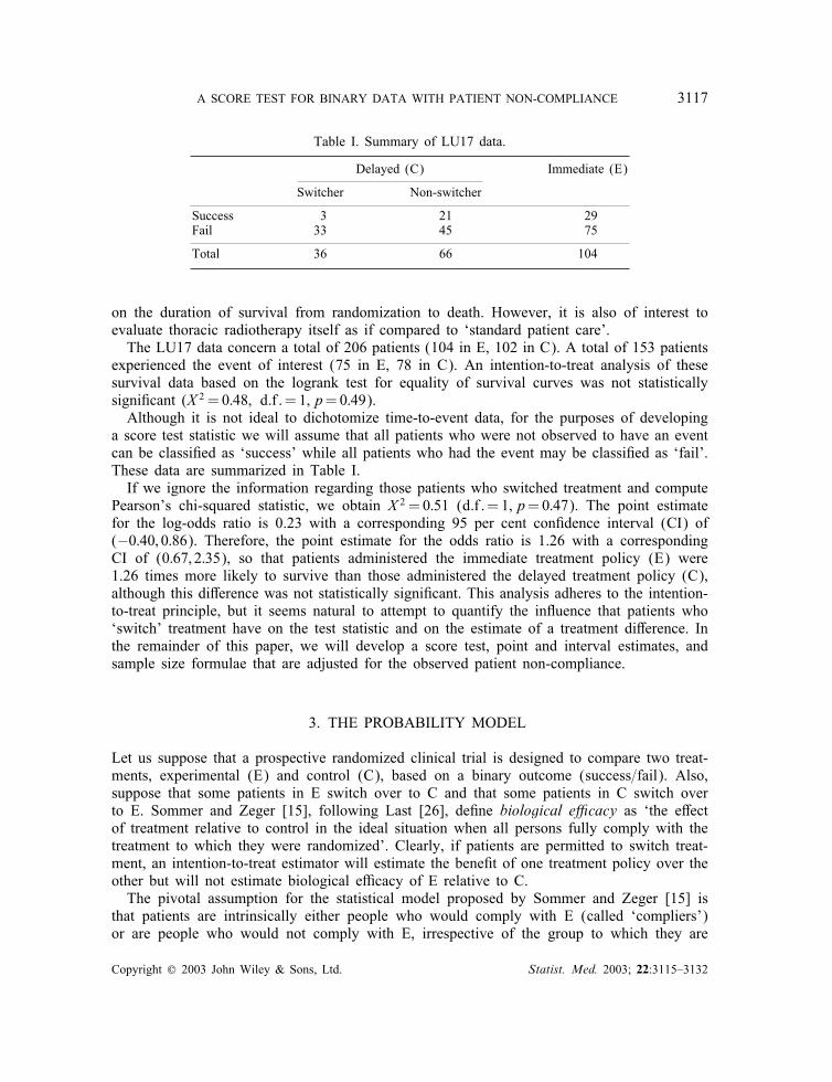
Table I. Summary of LU17 data.
Delayed (C) Immediate (E)
Switcher Non-switcher
Success 3 21 29Fail 33 45 75
Total 36 66 104
on the duration of survival from randomization to death. However, it is also of interest toevaluate thoracic radiotherapy itself as if compared to ‘standard patient care’.The LU17 data concern a total of 206 patients (104 in E, 102 in C). A total of 153 patients
experienced the event of interest (75 in E, 78 in C). An intention-to-treat analysis of thesesurvival data based on the logrank test for equality of survival curves was not statisticallysigni�cant (X 2 = 0:48; d:f :=1; p=0:49).Although it is not ideal to dichotomize time-to-event data, for the purposes of developing
a score test statistic we will assume that all patients who were not observed to have an eventcan be classi�ed as ‘success’ while all patients who had the event may be classi�ed as ‘fail’.These data are summarized in Table I.If we ignore the information regarding those patients who switched treatment and compute
Pearson’s chi-squared statistic, we obtain X 2 = 0:51 (d:f :=1; p=0:47). The point estimatefor the log-odds ratio is 0.23 with a corresponding 95 per cent con�dence interval (CI) of(−0:40; 0:86). Therefore, the point estimate for the odds ratio is 1.26 with a correspondingCI of (0:67; 2:35), so that patients administered the immediate treatment policy (E) were1.26 times more likely to survive than those administered the delayed treatment policy (C),although this di�erence was not statistically signi�cant. This analysis adheres to the intention-to-treat principle, but it seems natural to attempt to quantify the in�uence that patients who‘switch’ treatment have on the test statistic and on the estimate of a treatment di�erence. Inthe remainder of this paper, we will develop a score test, point and interval estimates, andsample size formulae that are adjusted for the observed patient non-compliance.
3. THE PROBABILITY MODEL
Let us suppose that a prospective randomized clinical trial is designed to compare two treat-ments, experimental (E) and control (C), based on a binary outcome (success=fail). Also,suppose that some patients in E switch over to C and that some patients in C switch overto E. Sommer and Zeger [15], following Last [26], de�ne biological e�cacy as ‘the e�ectof treatment relative to control in the ideal situation when all persons fully comply with thetreatment to which they were randomized’. Clearly, if patients are permitted to switch treat-ment, an intention-to-treat estimator will estimate the bene�t of one treatment policy over theother but will not estimate biological e�cacy of E relative to C.The pivotal assumption for the statistical model proposed by Sommer and Zeger [15] is
that patients are intrinsically either people who would comply with E (called ‘compliers’)or are people who would not comply with E, irrespective of the group to which they are
Copyright ? 2003 John Wiley & Sons, Ltd. Statist. Med. 2003; 22:3115–3132
3118 M. BRANSON AND J. WHITEHEAD
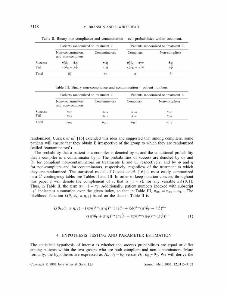
Table II. Binary non-compliance and contamination – cell probabilities within treatment.
Patients randomized to treatment C Patients randomized to treatment E
Non-contaminators Contaminators Compliers Non-compliersand non-compliers
Success ����C + ��� ��� ����E + ��� ���Fail ��� ��C + �� �� �� �� ��� ��E + �� �� �� ��
Total �� �� � ��
Table III. Binary non-compliance and contamination – patient numbers.
Patients randomized to treatment C Patients randomized to treatment E
Non-contaminators Contaminators Compliers Non-compliersand non-compliers
Success n000 n010 n100 n110Fail n001 n011 n101 n111
Total n00+ n01+ n10+ n11+
randomized. Cuzick et al. [16] extended this idea and suggested that among compilers, somepatients will ensure that they obtain E irrespective of the group to which they are randomized(called ‘contaminators’).The probability that a patient is a compiler is denoted by �, and the conditional probability
that a compiler is a contaminator by �. The probabilities of success are denoted by �E and�C for compliant non-contaminators on treatments E and C, respectively, and by � and �for non-compliers and for contaminators, respectively, regardless of the treatment to whichthey are randomized. The statistical model of Cuzick et al. [16] is most easily summarizedin a 24 contingency table: see Tables II and III. In order to keep notation concise, throughoutthis paper �s will denote the complement of s, that is (1 − s), for any variable s∈ (0; 1).Thus, in Table II, the term ��=1− ��. Additionally, patient numbers indexed with subscript‘+’ indicate a summation over the given index, so that in Table III, n00+ = n000 + n001. Thelikelihood function L(�E; �C; �; �; �) based on the data in Table II is
L(�E; �C; �; �; �) = (���)n010 (�� ��)n011 (����C + ���)n000 (��� ��C + �� ��)n001
×(����E + ���)n100 (��� ��E + �� ��)n101 ( ���)n110 ( �� ��)n111 (1)
4. HYPOTHESIS TESTING AND PARAMETER ESTIMATION
The statistical hypothesis of interest is whether the success probabilities are equal or di�eramong patients within the two groups who are both compliers and non-contaminators. Moreformally, the hypotheses are expressed as H0 : �E = �C versus H1 : �E �= �C. We will derive the
Copyright ? 2003 John Wiley & Sons, Ltd. Statist. Med. 2003; 22:3115–3132

A SCORE TEST FOR BINARY DATA WITH PATIENT NON-COMPLIANCE 3119
test statistics for the likelihood ratio test (LRT), Wald’s test and the score test. Throughoutthis paper, the parameter of interest is taken to be the log-odds ratio , where
= log{�E(1− �C)(1− �E)�C
}(2)
Thus, the null hypothesis corresponds to testing whether is equal to zero.
4.1. The likelihood ratio test
The LRT statistic for Cuzick’s model is equal to the log of the ratio of the likelihoodsmaximized under H0 and H1, and it will be denoted by WCZ. The derivation of maximumlikelihood estimates and of the LRT statistic can be found in Appendix A.For the statistical model summarized in Table II, the alternative hypothesis is not completely
unrestricted: it is that this statistical model holds with �E �=�C. Within constraints which ensurethat maximum likelihood estimates for all �ve parameters in Table II exist (see Appendix A,conditions (A1) and (A2)), WCZ is given by
WCZ =−2{n0++ log(n0++)− n0+0 log(n0+0)− n0+1 log(n0+1)
+n1++ log(n1++)− n1+0 log(n1+0)− n1+1 log(n1+1)
+ n++0 log(n++0) + n++1 log(n++1)− n+++ log(n+++)} (3)
To test H0, this is compared to a chi-squared distribution on one degree of freedom. If theconstraints of condition (A1) do not hold, then the maximum likelihood estimates under H1have to be found numerically, and similarly under H0, if the constraints of condition (A2) donot hold. If any cells are zero, then equation (3) is still valid, interpreting 0 log 0 to be zero(as limx→0+ x log x = 0).A standard intention-to-treat analysis of such data would ignore patient non-compliance and
contamination, and compare the groups as randomized. It is straightforward to show that theLRT statistic using an ITT analysis (WITT) is identical to that given in equation (3). Hence,WITT¿WCZ, with strict inequality if and only if either of the constraints (A1) or (A2) do nothold. Hence, the LRT from the binary non-compliance and contamination model has (slightly)less power for detecting a given treatment di�erence than the LRT of a standard ITT analysis.
4.2. Wald’s test
In Sommer and Zeger [15] and Cuzick et al. [16], the variance for the parameter of interestwas estimated using the ‘delta’ method. Wald’s test statistic is constructed as { ̂ =SE( ̂ )}2 andis compared to the appropriate critical value from the chi-squared distribution on one degreeof freedom. The details required to compute ̂ and SE( ̂ ) can be found in Appendix B.
4.3. The score test
To derive the score test, the likelihood function (1) is reparameterized in terms of the parame-ter of interest, , and a vector of nuisance parameters, ^. Following the approach of Whitehead
Copyright ? 2003 John Wiley & Sons, Ltd. Statist. Med. 2003; 22:3115–3132

3120 M. BRANSON AND J. WHITEHEAD
[27], denote the e�cient score of when =0 by Z , and denote observed Fisher’s informa-tion about Z by V . As is parameterized so that positive values imply E is better than C,positive values for Z also imply that E is better than C.The score test statistic is computed as Z2=V and is compared to the appropriate critical
value from a chi-squared distribution on one degree of freedom.
4.3.1. The score test: An Intention-to-Treat analysis In this case, Table II reduces to a 2× 2contingency table concerning the ‘overall’ success probability for treatment policies E and C.The intention-to-treat score test statistics can be written as
ZITT =−n1+1 + n1++p̂f and VITT = n0++n1++n++0n++1=n3+++ (4)
where pf is the probability of failure under H0 and its maximum likelihood estimate p̂f issimply the total number of patients who failed (n++1) divided by the total number of patients(n+++). We denote the corresponding probability of success ps = 1 − pf which is estimatedby n++0=n+++. Notice that Z2ITT=VITT is equal to Pearson’s chi-squared statistic
∑(O−E)2=E.
4.3.2. The score test: Adjusted for binary non-compliance and contamination Using thelikelihood function in (1), the e�cient score (ZCZ) for the model suggested by Cuzick et al.[16] can be shown to be related to the standard ITT e�cient score in (4) according to
ZCZ =ZITT( n100n1+0
− n010n0+0)( n101
n1+1− n011
n0+1)
p̂s(n100n1+0
− n010n0+0) + p̂f (
n101n1+1
− n011n0+1)
(5)
Using (A5), Fisher’s information (VCZ) is given by
VCZ =VITT
{( n100n1+0
− n010n0+0)( n101
n1+1− n011
n0+1)
p̂s(n100n1+0
− n010n0+0) + p̂f (
n101n1+1
− n011n0+1)
}2(6)
provided that constraint (A2) holds. To test the null hypothesis, we construct the score teststatistic Z2CZ=VCZ and from (5) and (6)
Z2CZ=VCZ =Z2ITT=VITT (7)
Details of these derivations are given in Appendix C.The result above shows that, provided that constraint (A2) holds, the score test using the
binary non-compliance and contamination model due to Cuzick et al. [16] provides identicalresults to a standard ITT analysis. If these constraints are violated, then we might rule thatCuzick’s method should not lead to rejection of H0, while the intention-to-treat method maydo so. With such a convention, the score test for the binary non-compliance and contaminationmodel has less power than the corresponding score test for the ‘standard’ ITT analysis althoughthe actual di�erence is small – as we will demonstrate in Section 6.
4.4. Special cases: Binary non-compliance or binary contamination
The model suggested by Cuzick et al. [16] is a generalization of the model originally suggestedby Sommer and Zeger [15]. If the incidence of observable contamination in C is zero, theCuzick model reduces to that earlier model. If the incidence of observable non-compliance
Copyright ? 2003 John Wiley & Sons, Ltd. Statist. Med. 2003; 22:3115–3132
A SCORE TEST FOR BINARY DATA WITH PATIENT NON-COMPLIANCE 3121
in E is zero, then the Cuzick model may be described as a simple contamination model. Themultiplication factor of ZITT in (5) may be written as{
p̂s
(n101n1+1
− n011n0+1
)−1+ p̂f
(n100n1+0
− n010n0+0
)−1}−1(8)
In the case of simple binary non-compliance, as studied by Sommer and Zeger [15], thismultiplication factor reduces to
{p̂s
(n1+1n101
)+ p̂f
(n1+0n100
)}−1(9)
For the simple binary contamination model, it reduces to
{p̂s
(n0+1n001
)+ p̂f
(n0+0n000
)}−1(10)
5. SAMPLE SIZE ESTIMATION
Following the approach and notation of Whitehead [27], de�ne the reference improvement( R) as the magnitude of treatment di�erence that one wishes to detect in the clinical trial.When there is no di�erence between the two treatments ( =0), the probability of rejectingH0 is denoted by � (the type I error rate). When = R, the probability of rejecting H1 isto be 1− � (the power).In large samples, Z ∼ N(0; V ) under the null hypothesis, while Z ∼ N( RV; V ), under the
alternative hypothesis. The requirements of the test are
P(Z¿k; =0)=�2
and P(Z¿k; = R)=1− �
and they are satis�ed by choosing V and k as
V =(U�=2 +U�
R
)2and k=
(U�=2 +U�)U�=2
R(11)
where U� denotes the upper 100(1− �) percentage point of the standard normal distribution.To obtain the sample size, an equation linking Fisher’s information to the total number of
patients in the study is required. For the intention-to-treat analysis, assuming large samples,n++0≈ n+++ps, n++1≈ n+++pf , n1++≈ n+++R=(R +1), and n0++≈ n+++=(R +1), where R : 1is the allocation ratio E :C, Fisher’s information (VITT) given by (4), becomes
VITT≈ R(R + 1)2
pspfn+++ (12)
From (11), the sample size n+++ needed to yield the required amount of information, can befound. The parameter estimated in an ITT analysis ( ′) is given in terms of more general
Copyright ? 2003 John Wiley & Sons, Ltd. Statist. Med. 2003; 22:3115–3132
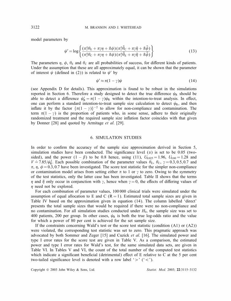
3122 M. BRANSON AND J. WHITEHEAD
model parameters by
′= log
{(����E + ���+ ���) (��� ��C + �� ��+ �� ��)
(����C + ���+ ���) (��� ��E + �� ��+ �� ��)
}(13)
The parameters �, �, �E and �C are all probabilities of success, for di�erent kinds of patients.Under the assumption that these are all approximately equal, it can be shown that the parameterof interest (de�ned in (2)) is related to ′ by
′ ≈�(1− �) (14)
(see Appendix D for details). This approximation is found to be robust in the simulationsreported in Section 6. Therefore a study designed to detect the true di�erence R should beable to detect a di�erence ′
R =�(1 − �) R within the intention-to-treat analysis. In e�ect,one can perform a standard intention-to-treat sample size calculation to detect R, and thenin�ate it by the factor {�(1 − �)}−2 to allow for non-compliance and contamination. Theterm �(1 − �) is the proportion of patients who, in some sense, adhere to their originallyrandomized treatment and the required sample size in�ation factor coincides with that givenby Donner [28] and quoted by Armitage et al. [29].
6. SIMULATION STUDIES
In order to con�rm the accuracy of the sample size approximation derived in Section 5,simulation studies have been conducted. The signi�cance level (�) is set to be 0.05 (two-sided), and the power (1 − �) to be 0.8 hence, using (11), U0:025 = 1:96, U0:80 = 1:28 andV :=7:85= 2R. Each possible combination of the parameter values �E, �C, �=0:3; 0:5; 0:7 and�, �, �=0:3; 0:7 have been investigated. The score test statistic for the simpler non-complianceor contamination model arises from setting either � to 1 or � to zero. Owing to the symmetryof the test statistics, only the latter case has been investigated. Table II shows that the terms� and �� only occur in conjunction with �, hence when �=0, the e�ects of di�ering values of� need not be explored.For each combination of parameter values, 100 000 clinical trials were simulated under the
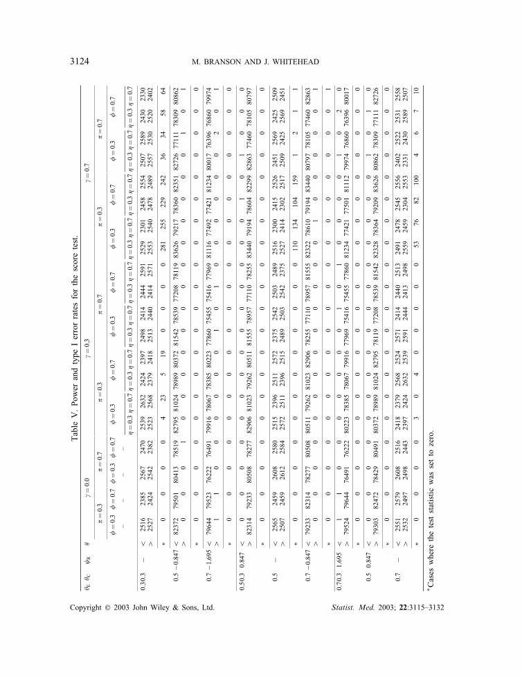
assumption of equal allocation to E and C (R=1). Estimated total sample sizes are given inTable IV based on the approximation given in equation (14). The column labelled ‘direct’presents the total sample sizes that would be required if there were no non-compliance andno contamination. For all simulation studies conducted under H0, the sample size was set to400 patients, 200 per group. In other cases, R is both the true log-odds ratio and the valuefor which a power of 80 per cent is achieved for the set sample size.If the constraints concerning Wald’s test or the score test statistic (condition (A1) or (A2))
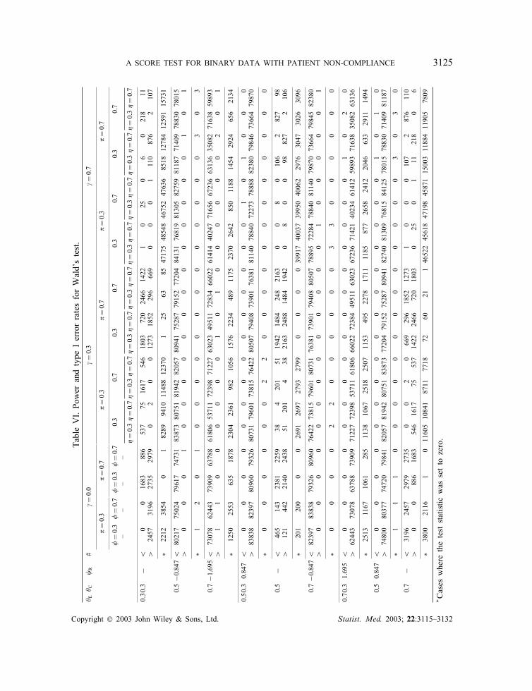
were violated, the corresponding test statistic was set to zero. This pragmatic approach wasadvocated by both Sommer and Zeger [15] and Cuzick et al. [16]. The simulated power andtype I error rates for the score test are given in Table V. As a comparison, the estimatedpower and type I error rates for Wald’s test, for the same simulated data sets, are given inTable VI. In Tables V and VI, the count of the total number of the computed test statisticswhich indicate a signi�cant bene�cial (detrimental) e�ect of E relative to C at the 5 per centtwo-tailed signi�cance level is denoted with a row label ‘¿’ (‘¡’).
Copyright ? 2003 John Wiley & Sons, Ltd. Statist. Med. 2003; 22:3115–3132
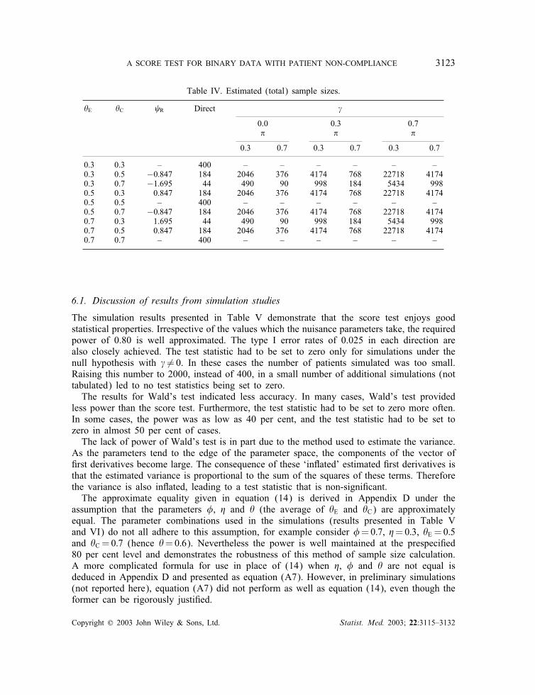
A SCORE TEST FOR BINARY DATA WITH PATIENT NON-COMPLIANCE 3123
Table IV. Estimated (total) sample sizes.
�E �C R Direct �
0.0 0.3 0.7� � �
0.3 0.7 0.3 0.7 0.3 0.7
0.3 0.3 – 400 – – – – – –0.3 0.5 −0:847 184 2046 376 4174 768 22718 41740.3 0.7 −1:695 44 490 90 998 184 5434 9980.5 0.3 0.847 184 2046 376 4174 768 22718 41740.5 0.5 – 400 – – – – – –0.5 0.7 −0:847 184 2046 376 4174 768 22718 41740.7 0.3 1.695 44 490 90 998 184 5434 9980.7 0.5 0.847 184 2046 376 4174 768 22718 41740.7 0.7 – 400 – – – – – –
6.1. Discussion of results from simulation studies
The simulation results presented in Table V demonstrate that the score test enjoys goodstatistical properties. Irrespective of the values which the nuisance parameters take, the requiredpower of 0.80 is well approximated. The type I error rates of 0.025 in each direction arealso closely achieved. The test statistic had to be set to zero only for simulations under thenull hypothesis with � �=0. In these cases the number of patients simulated was too small.Raising this number to 2000, instead of 400, in a small number of additional simulations (nottabulated) led to no test statistics being set to zero.The results for Wald’s test indicated less accuracy. In many cases, Wald’s test provided
less power than the score test. Furthermore, the test statistic had to be set to zero more often.In some cases, the power was as low as 40 per cent, and the test statistic had to be set tozero in almost 50 per cent of cases.The lack of power of Wald’s test is in part due to the method used to estimate the variance.
As the parameters tend to the edge of the parameter space, the components of the vector of�rst derivatives become large. The consequence of these ‘in�ated’ estimated �rst derivatives isthat the estimated variance is proportional to the sum of the squares of these terms. Thereforethe variance is also in�ated, leading to a test statistic that is non-signi�cant.The approximate equality given in equation (14) is derived in Appendix D under the
assumption that the parameters �, � and � (the average of �E and �C) are approximatelyequal. The parameter combinations used in the simulations (results presented in Table Vand VI) do not all adhere to this assumption, for example consider �=0:7, �=0:3, �E =0:5and �C =0:7 (hence �=0:6). Nevertheless the power is well maintained at the prespeci�ed80 per cent level and demonstrates the robustness of this method of sample size calculation.A more complicated formula for use in place of (14) when �, � and � are not equal isdeduced in Appendix D and presented as equation (A7). However, in preliminary simulations(not reported here), equation (A7) did not perform as well as equation (14), even though theformer can be rigorously justi�ed.
Copyright ? 2003 John Wiley & Sons, Ltd. Statist. Med. 2003; 22:3115–3132
3124 M. BRANSON AND J. WHITEHEAD
TableV.PowerandtypeIerrorratesforthescoretest.
� E� C
R
#�=0:0
�=0:3
�=0:7
�=0:3
�=0:7
�=0:3
�=0:7
�=0:3
�=0:7
�=0:3
�=0:7
�=0:3
�=0:7
�=0:3
�=0:7
�=0:3
�=0:7
�=0:3
�=0:7
�=0:3
�=0:7
––
––
�=0:3�=0:7�=0:3�=0:7�=0:3�=0:7�=0:3�=0:7�=0:3�=0:7�=0:3�=0:7�=0:3�=0:7�=0:3�=0:7
0.30.3
−¡
2516
2385
2567
2470
2539
2632
2424
2397
2498
2414
2444
2591
2529
2301
2458
2554
2507
2589
2430
2330
¿2527
2424
2542
2382
2523
2568
2379
2418
2513
2440
2414
2571
2553
2540
2478
2489
2557
2530
2520
2402
∗0
00
04
235
190
00
0281
255
229
242
3634
5864
0.5−0:847¡
82372
79501
80413
7851982795810247898980372815427853977208781198362679217783608235182726771117830980862
¿0
00
10
00
00
00
00
00
00
10
1
∗0
00
00
00
00
00
00
00
00
00
0
0.7−1:695¡
79644
79523
76222
7649179916780677838580223778607545575416779698111677492774218123480017763967686079974
¿1
10
00
00
01
01
00
00
00
20
1
∗0
00
00
00
00
00
00
00
00
00
0
0.50.30.847
¡0
00
00
00
00
00
00
01
01
00
0¿
82314
79233
80508
7827782906810237926280511815557895777110782558344079194786048229982863774607810580797
∗0
00
00
00
00
00
00
00
00
00
0
0.5
−¡
2565
2459
2608
2580
2515
2396
2511
2572
2375
2542
2503
2489
2516
2300
2415
2526
2451
2569
2425
2509
¿2507
2459
2612
2584
2572
2511
2396
2515
2489
2503
2542
2375
2527
2414
2302
2517
2509
2425
2569
2451
∗0
00
00
00
00
00
0110
134
104
159
12
11
0.7−0:847¡
79233
82314
78277
8050880511792628102382906782557711078957815558232278610791948344080797781057746082863
¿0
00
00
00
00
00
00
10
00
00
1
∗0
00
00
00
00
00
00
00
00
00
1
0.70.31.695
¡1
10
00
00
00
10
10
00
01
02
0¿
79524
79644
76491
7622280223783857806779916779697541675455778608123477421775018111279974768607639680017
∗0
00
00
00
00
00
00
00
00
00
0
0.50.847
¡0
00
00
00
00
00
00
00
01
01
0¿
79303
82472
78429
8049180372789898102482795781197720878539815428232878364792098362680862783097711182726
∗0
00
00
00
00
00
00
00
00
00
0
0.7
−¡
2551
2579
2608
2516
2418
2379
2568
2524
2571
2414
2440
2513
2491
2478
2545
2556
2402
2522
2531
2558
¿2532
2497
2498
2443
2397
2424
2632
2539
2591
2444
2413
2498
2559
2459
2304
2553
2331
2430
2589
2507
∗0
00
03
04
00
00
053
7682
100
46
710
∗ Caseswheretheteststatisticwassettozero.
Copyright ? 2003 John Wiley & Sons, Ltd. Statist. Med. 2003; 22:3115–3132
A SCORE TEST FOR BINARY DATA WITH PATIENT NON-COMPLIANCE 3125TableVI.PowerandtypeIerrorratesforWald’stest.
� E� C
R
#�=0:0
�=0:3
�=0:7
�=0:3
�=0:7
�=0:3
�=0:7
�=0:3
�=0:7
�=0:3
�=0:7
�=0:3
�=0:7
0:3
0:7
0:3
0:7
0:3
0:7
0:3
0:7
––
––
�=0:3�=0:7�=0:3�=0:7�=0:3�=0:7�=0:3�=0:7�=0:3�=0:7�=0:3�=0:7�=0:3�=0:7�=0:3�=0:7
0.30.3
−¡
00
1683
886
537
751617
546
1803
720
2466
1422
10
250
60
218
11¿
2457
3196
2735
2979
02
00
1273
1852
296
669
00
01
110
876
2107
∗2212
3854
01
8289
9410
1148812370
125
6385
47175485484675247636
8518
127841259115731
0.5−0:847¡
80217
75024
79617
7473183873807518194282057809417528779152772048413176819813058275981187714097883078015
¿0
00
10
00
00
00
00
00
00
10
1
∗1
20
10
00
00
00
00
00
00
30
3
0.7−1:695¡
73078
62443
73909
6378861806537117239871227630234951172834660226141440247716566723663136350827163859893
¿1
10
00
00
01
01
00
00
00
20
1
∗1250
2553
635
1878
2304
2361
982
1056
1576
2234
489
1175
2370
2642
850
1188
1454
2924
656
2134
0.50.30.847
¡0
00
00
00
00
00
00
01
01
00
0¿
83838
82397
80960
7932680731796017381576422805077940873901763818114078840722737888882380798467366479870
∗0
00
00
02
20
00
00
00
00
00
0
0.5
−¡
465
143
2381
2259
384
201
511942
1484
248
2163
00
80
106
2827
98¿
121
442
2140
2438
51201
438
2163
2488
1484
1942
08
00
98827
2106
∗201
200
00
2691
2697
2793
2799
00
0039917400373995040062
2976
3047
3026
3096
0.7−0:847¡
82397
83838
79326
8096076422738157960180731763817390179408805077889572284788408114079870736647984582380
¿0
00
00
00
00
00
00
10
00
00
1
∗0
00
02
20
00
00
03
30
00
00
0
0.70.31.695
¡0
00
00
00
00
00
00
00
01
02
0¿
62443
73078
63788
7390971227723985371161806660227238449511630236723671421402346141259893716383508263136
∗2513
1167
1061
285
1138
1067
2518
2507
1153
495
2278
1711
1185
877
2658
2412
2046
633
2911
1494
0.50.847
¡0
00
00
00
00
00
00
00
01
01
0¿
74800
80377
74720
7984182057819428075183873772047915275287809418274081309768158412578015788307140981187
∗1
11
00
00
00
00
00
00
03
03
0
0.7
−¡
3196
2457
2979
2735
00
20
669
296
1852
1273
10
00
107
2876
110
¿0
0886
1683
546
1617
75537
1422
2466
720
1803
025
01
11218
06
∗3800
2116
101160510841
8711
7718
7260
21146522456184719845871150031188411905
7809
∗ Caseswheretheteststatisticwassettozero.
Copyright ? 2003 John Wiley & Sons, Ltd. Statist. Med. 2003; 22:3115–3132
3126 M. BRANSON AND J. WHITEHEAD
7. REANALYSIS OF LU17
The data presented in Table I provide an example of a simple contamination model, and anintention-to-treat analysis was presented in Section 2.The adjusted chi-squared score test statistic for this simple binary contamination model is
the same as that presented in Section 2, namely, X 2 = 0:51 (d:f :=1, p=0:47). The adjustedpoint estimate and corresponding 95 per cent CI for may be obtained using equation (A3)and (A4) as 0.30 and (−0:52; 1:11), respectively. Thus, the estimated odds ratio is 1.34 witha corresponding CI (0:60; 3:03). As is small, an approximate point estimate and 95 percent CI for are given by Z=V and (Z=V − 1:96=√V ; Z=V +1:96=
√V ), with values 0.30 and
(−0:51; 1:10), respectively. In this case the approximation is good.
8. DISCUSSION
The primary analysis of data arising from randomized clinical trials should adhere to theintention-to-treat principle, even when non-compliance and=or contamination has occurred.Supplementary analyses that adjust for the features can then be investigated. Adjusting forobserved non-compliance provides an estimate of biological e�cacy rather than di�erencebetween treatment policies. For the LU17 data set, the adjusted point estimate was 1.34compared with an initial estimate of 1.26. As the correct p-value for the adjusted analysisis the same as that of the intention-to-treat analysis, it follows that while the point estimatemay better re�ect the biological e�cacy of experimental to control treatment, its precision isdecreased. No gain in power is possible by adjusting for patient non-compliance.The work in this paper was motivated by a simple presentation of Sommer and Zeger’s
approach given by Cox [31] in a discussion of a paper by Rubin [32]. Rubin’s methoddeals with more general data types than just binary [32, 33] and is based on randomizationanalyses. However, after acknowledging the clever technical achievements of Rubin’s paper,Cox listed the advantages of the Sommer and Zeger method as being simpler computation,greater transparency, the possibility of deriving associated con�dence intervals and ease ofextension to Bayesian versions and of allowing for covariates. For these reasons, we choseto follow the Sommer and Zeger approach.Sommer and Zeger and Cuzick et al. recommended using Wald’s test. The simulation results
presented in this paper show that this test statistic is not appropriate, since the observed errorrates are not maintained at the prescribed levels. Furthermore, Cuzick et al. suggest that theadjusted test statistic may deliver more power relative to the intention-to-treat analysis forcertain combinations of parameter values. We have shown that such a gain in power is notpossible. Furthermore, we have shown that the adjusted test statistic has power equal to theintention-to-treat analysis – given that the sample size was chosen appropriately.In Section 5, a sample size approximation was introduced via equation (14) that imposed
what might appear to be a strong assumption regarding approximate equality of certain nui-sance parameters. Simulations reported in Section 6 show that this simple approximation canbe e�ective, even when the assumption under which it is justi�ed in Appendix D is violated.Further investigation of why this is so would be of interest.Sommer and Zeger and Cuzick et al. parameterized treatment di�erence using the log
relative risk. The statistics Z and V based on the log relative risk can be shown to be
Copyright ? 2003 John Wiley & Sons, Ltd. Statist. Med. 2003; 22:3115–3132
A SCORE TEST FOR BINARY DATA WITH PATIENT NON-COMPLIANCE 3127
identical to those of the intention-to-treat score test as given in equation (4), provided thatcondition (A2) in Appendix A holds. Thus, the simulation results presented in this paper arealso relevant to the score test for the log relative risk. The invariance of the score test toreparameterization is as expected since both the score test and the likelihood ratio test areboth invariant to reparameterization [30].The score test is easily generalized to allow for strati�cation, simply computing Z =
∑Kk=1 Zk
and V =∑K
k=1 Vk , where Zk and Vk are the stratum speci�c e�cient scores and observedFisher’s information, respectively. The formal test of H0 is then performed by comparingZ 2=V to the appropriate critical value from a 21 distribution.
APPENDIX A: MAXIMUM LIKELIHOOD ESTIMATION AND THELIKELIHOOD RATIO TEST
A.1. Maximum likelihood under H1
Under the alternative hypothesis H1 each cell probability in Table II (denoted by pijk fori; j; k=0; 1) is simply estimated by a proportion based on Table III. For example ��� (=p010)is estimated by n010=n0++ and ����E + ��� (=p100) is estimated by n100=n1++. As ����E¿0,the second of these expressions must be greater than or equal to the �rst, and the straight-forward method of estimation breaks down if n010=n0++¿n100=n1++. As patients who wouldbe contaminators usually form a small subset of those who would be compilers, the above(strict) inequality is unlikely to hold, especially as sample sizes increase in size. The fullset of constraints under which each cell probability can be estimated by the correspondingobserved proportion is given by condition (A1)
n000n0++
¿n110n1++
;n001n0++
¿n111n1++
;n100n1++
¿n010n0++
;n101n1++
¿n011n0++
(A1)
Eight probabilities have been de�ned under H1 yet there are only 6 degrees of freedom. Itis clear that given any three estimated probabilities for either E or C, the fourth probabilityis equal to one minus the sum of these three.
A.2. Maximum likelihood under H0
Under the null hypothesis only 5 of the maximum 6 degrees of freedom are available. The(unrestricted) maximum likelihood estimates under H0 (denoted by p̃ijk) are given by
p̃100 = p̂sn100n1+0
; p̃110 = p̂sn110n1+0
; p̃111 = p̂fn111n1+1
; p̃010 = p̂sn010n0+0
; p̃011 = p̂fn011n0+1
where p̂s and p̂f are maximum likelihood estimates for the overall probability of success(= n++0=n+++) and failure (= n++1=n+++), respectively. All other probabilities can be obtainedfrom a linear combination of the probabilities dealt with above. As in the case of estimationunder H1, p̃100 has to be greater than or equal to p̃010. If this inequality does not hold, thestraightforward method of estimation breaks down. The full set of constraints are given incondition (A2)
n100n1+0
¿n010n0+0
andn101n1+1
¿n011n0+1
(A2)
Copyright ? 2003 John Wiley & Sons, Ltd. Statist. Med. 2003; 22:3115–3132

3128 M. BRANSON AND J. WHITEHEAD
A.3. The likelihood ratio test statistic
The log-likelihood function under H0 (‘0) is
‘0 =1∑
i; j; k=0nijk{log(nijk) + log(n++k)− log(ni+k)− log(n+++)}
Under H1, the log-likelihood function (‘1) is given by
‘1 =1∑
i; j; k=0nijk log(nijk)− n0++ log(n0++)− n1++ log(n1++)
The likelihood ratio test statistic (WCZ) in equation (3) is then obtained by calculating−2(‘0 − ‘1).
APPENDIX B: WALD’S TEST
The parameter of interest was de�ned in equation (2). Re-expressing as a function ofthe pijk’s, we note that
= log{
(p100 − p010)(p101 + p000 + p001 + p010 − 1)
(p100 + p101 + p110 + p001 − 1)(p000 − p110)
}(A3)
The maximum likelihood estimate for ( ̂ ) is obtained by substituting the maximum likeli-hood estimates for pijk , (i; j; k=0; 1) (see Appendix A for details) into equation (A3).In general, the delta method is implemented as follows. Suppose that the variance matrix for
a set of parameters (!̂i : i=1; : : : ; n) is estimated by var(!̂). Let a function of these parametersf(!i : i=1; : : : ; n) be denoted f(!), and represent the row vector of �rst derivatives of f(!),with respect to !i, i=1; : : : ; n, by �. The variance estimate for f(!̂) is given by
var(f(!̂))≈�var(!̂)�T (A4)
In our case =f(!), and Wald’s test statistic is constructed as { ̂ =SE( ̂ )}2 and is comparedto the appropriate critical value from the chi-squared distribution on one degree of freedom.Therefore, the components of �, the row vector of �rst derivatives of with respect to pijk ,are
@ @p100
=1
p100 − p010+
1p100 + p101 + p110 + p001 − 1
@ @p101
=1
p100 + p101 + p110 + p001 − 1 − 1p101 + p000 + p001 + p010 − 1
(=
@ @p001
)
@ @p110
=1
p100 + p101 + p110 + p001 − 1 +1
p000 − p110
(=− @
@p000
)
@ @p010
=1
p100 − p010+
1p101 + p000 + p001 + p010 − 1
Copyright ? 2003 John Wiley & Sons, Ltd. Statist. Med. 2003; 22:3115–3132

A SCORE TEST FOR BINARY DATA WITH PATIENT NON-COMPLIANCE 3129
The variance matrix for (p̂100; p̂101; p̂110; p̂000; p̂001; p̂010) is obtained assuming independentmultinomial sampling and has the form
var(p̂)=
(P1 00 P2
)
where the submatrix P1 is given by
P1 =
p100(1− p100)=n1++ −p100p101=n1++ −p100p110=n1++
−p100p101=n1++ p101(1− p101)=n1++ −p101p110=n1++
−p100p110=n1++ −p101p110=n1++ p110(1− p110)=n1++
The submatrix P2 is given similarly with p100, p101 and p110 replaced with p000, p001 andp010, respectively, and n1++ by n0++. The variance is then obtained from equation (A4) in astraightforward manner.
APPENDIX C: THE SCORE TEST
We �rst determine Fisher’s observed information: we employ equation (A4) to estimate thevariance for , but substitute the parameter estimates under H0 into the (row) vector of�rst derivatives �, to obtain �H0 , and into the variance matrix (var(!̂)) to obtain varH0 (!̂).Fisher’s observed information (V ) is then estimated using the following equation:
V−1≈�H0 varH0 (!̂)�TH0 (A5)
It can be deduced from Appendix B that �̂H0 = (�̂; 0; �̂;−�̂; 0;−�̂) where �̂=(p̃100−p̃010)−1+
(1− p̃100 − p̃110 − p̃111 − p̃011)−1. Therefore, with a little simpli�cation
varH0 ( ̂ ) = �̂H0 varH0 (p̂)�̂TH0
= �̂2p̂sp̂fn+++
n1++n0++
Now, VCZ is found by inverting varH0 ( ̂ ), and it follows that
VCZ =VITT1
(p̂sp̂f �̂)2
Now, �̂ = p̂−1s (
n100n1+0
− n010n0+0)−1 + p̂−1
f (n101n1+1
− n011n0+1)−1, giving
VCZ = VITT
{p̂f
(n100n1+0
− n010n0+0
)−1+ p̂s
(n101n1+1
− n011n0+1
)−1}−2
Copyright ? 2003 John Wiley & Sons, Ltd. Statist. Med. 2003; 22:3115–3132

3130 M. BRANSON AND J. WHITEHEAD
= VITT
(n100n1+0
− n010n0+0
)+(
n101n1+1
− n011n0+1
)
p̂s
(n100n1+0
− n010n0+0
)+ p̂f
(n101n1+1
− n011n0+1
)
2
as given in equation (6).To determine ZCZ, the likelihood function given in equation (1) is reparameterized in terms
of the parameter of interest, , and a vector of nuisance parameters, ^. Let us de�ne
1 = log(
�C1− �C
); 2 =�; 3 = �; 4 = �
Thus, �E = e +1
1+e +1, �C = e1
1+e1and under H0, �E = �C = � (say). The likelihood function (‘) as
a function of is
‘∝ n100 log{2(1− 3)e +1 + 234(1 + e +1)}
+ n101 log{2(1− 3) + 23(1− 4) (1 + e +1)} − n10+ log(1 + e +1)
Di�erentiating ‘ with respect to and putting =0 (that is, computing ZCZ) gives
ZCZ = �{n100
2(1− 3) + 2342(1− 3)�+ 234
+ n10123(1− 4)
2(1− 3) (1− �) + 23(1− 4)− n10+
}
By substituting the maximum likelihood estimates under H0 (details in Appendix A) for ^gives
ZCZ =(p̃100 + p̃010) (1− p̃100 − p̃110 − p̃111 − p̃011)
(1− p̃110 − p̃111 − p̃010 − p̃011)p̂sp̂f(n1+0 − n1++p̂s)
Now, (p̃100+p̃010) (1−p̃100−p̃110−p̃111−p̃011)(1−p̃110−p̃111−p̃010−p̃011)p̂sp̂f
= 1p̂sp̂f �̂
and n1+0 − n1++p̂s =− n1+1 + n1++p̂f , thus we havethe result as given in equation (5).
APPENDIX D: SAMPLE SIZE APPROXIMATION
Note, from equations (5) and (6), that ZCZ and VCZ are of the form
ZCZ = �ZITT and VCZ = �2VITT
where � is given by
�−1 = p̂f
(n100n1+0
− n010n0+0
)−1+ p̂s
(n101n1+1
− n011n0+1
)−1(A6)
Copyright ? 2003 John Wiley & Sons, Ltd. Statist. Med. 2003; 22:3115–3132

A SCORE TEST FOR BINARY DATA WITH PATIENT NON-COMPLIANCE 3131
Now
ZCZ∼N( CZVCZ; VCZ) and ZITT∼N( ITTVITT; VITT)so that
�ZITT∼N( ITT�VITT; �2VITT)which is
ZCZ∼N( ITT�
VCZ; VCZ
)
Thus, CZ = ITT=�. It follows that the sample size required to detect CZ = R will be �−2 timesthat calculated for the detection of ITT, naively ignoring non-compliance and contamination.In large samples
�−1 = (����+ ���+ ���)(��� ��+ �� ��+ �� ��)(1
��� ��+
1����
)
= (����+ ���+ ���)(�����+ �� ��+ �� ��){���� ��}−1 (A7)
If �=1 and �=0 (no contamination or non-compliance) then �−1 = 1. If �=�= � (all successprobabilities equal) then �−1 = {�(1− �)}−1, thus
ITT≈�(1− �) CZ
ACKNOWLEDGEMENTS
The �rst author was funded by MRC grant G78=5359. The authors are grateful to the MRC Cancertrials unit for provision of the data described in Section 2. The authors also thank the referees for theirhelpful comments and suggestions.
REFERENCES
1. Statistics in Medicine. Analysing non-compliance in clinical trials. Statistics in Medicine 1998; 17(3):247–393.
2. Robins J, Tsiatis A. Correcting for non-compliance in randomised trials using rank preserving structure failuretime models. Communications in Statistics – Theory and Methods 1991; 20:2609–2631.
3. Robins J. Estimation of the time-dependent accelerated failure time model in the presence of confounding factors.Biometrika 1992; 79:321–334.
4. Robins J, Tsiatis A. Semiparametric estimation of an accelerated failure time model with time-dependentcovariates. Biometrika 1992; 79:311–319.
5. Mark S, Robins J. Estimating the causal e�ect of smoking cessation in the presence of confounding factorsusing a rank preserving structural failure time model. Statistics in Medicine 1993; 12:1605–1628.
6. Mark S, Robins J. A method for the analysis of randomised trials with compliance information: an applicationto the multiple risk factor intervention trial. Controlled Clinical Trials 1993; 14:79–97.
7. Robins J, Greenland S. Adjusting for di�erential rates of prophylaxis therapy for PCP in high-dose versus low-dose AZT treatment arms in an AIDS randomised trial. Journal of the American Statistical Association 1994;89:737–749.
8. Rubin DR. Estimating causal e�ects of treatment in randomized and nonrandomized studies. Journal ofEducational Psychology 1974; 5:688–701.
9. Holland P. Statistics and causal inference. Journal of the American Statistical Association 1986; 81:945–970.
Copyright ? 2003 John Wiley & Sons, Ltd. Statist. Med. 2003; 22:3115–3132

3132 M. BRANSON AND J. WHITEHEAD
10. White IR, Walker S, Babiker AG, Darbvshire JH. Impact of treatment changes on the interpretation of theConcorde trial. AIDS 1997; 11:999–1006.
11. White IR, Goetghebeur EJT. Clinical trials comparing two treatment policies: which aspects of the treatmentpolicies makes a di�erence? Statistics in Medicine 1998; 17:319–339.
12. White IR, Babiker AG, Walker S, Darbyshire JH. Randomization-based methods for correcting for treatmentchanges: examples from the Concorde trial. Statistics in Medicine 1999; 18:2617–2634.
13. Branson M, Whitehead J. Estimating a treatment e�ect in survival studies in which patients switch treatment.Statistics in Medicine 2001; 21:2449–2463.
14. Baker SG. Analysis of survival data from a randomized trial with all-or-none compliance: estimating thecost-e�ectiveness of a cancer screening program. Journal of the American Statistical Association 1998; 93:929–934.
15. Sommer A, Zeger SL. On estimating e�cacy from clinical trials. Statistics in Medicine 1991; 10:45–52.16. Cuzick J, Edwards R, Segnan N. Adjusting for non-compliance and contamination in randomised clinical trials.
Statistics in Medicine 1997; 16:1017–1029.17. Sato T. A further look at the Cochran-Mantel-Haenzel risk di�erence. Controlled Clinical Trials 1995; 16:
359–361.18. Sato T. Sample size calculations with compliance information. Statistics in Medicine 2000; 19:2689–2697.19. Goetghebeur E, Molenberghs G, Katz J. Estimating the causal e�ect of compliance on binary outcome in
randomised controlled trials. Statistics in Medicine 1998; 17:341–355.20. Frangakis CE, Rubin DB. Addressing complications of intention-to-treat analysis in the combined presence of
all-or-none treatment non-compliance and subsequent missing outcomes. Biometrika 1999; 86:365–379.21. Falk SJ, White RJ, Hopwood P, Girling DJ, Sambrock RJ, Harvey A, Qian W, Stephens RJ. S53 Immediate
versus delayed thoracic radiotherapy (trt) in patients with unresectable advanced non-small cell lung cancer(NSCLC) and minimal symptoms: results of an MRC=BTS randomised trial. Thorax 1999; 53, Supplement3:A14.
22. Phillips TL, Miller RJ. Should asymptomatic patients with inoperable bronchogenic carcinoma receive immediateradiotherapy? YES. American Review of Respiratory Disease 1978; 117:405–410.
23. Cox JD, Komaki R, Byhardt RW. Is immediate chest radiotherapy obligatory for any or all patients withlimited-stage non-small cell carcinoma of the lung? Yes. Cancer Treatment Reports 1983; 67:327–331.
24. Brashear RE. Should asymptomatic patients with inoperable bronchogenic carcinoma receive immediateradiotherapy? NO. American Review of Respiratory Disease 1978; 117:411–414.
25. Cohen MH. Is immediate radiation therapy indicated for patients with unresectable non-small cell lung cancer?No. Cancer Treatment Reports 1983; 67:333–336.
26. Last JM. A Dictionary of Epidemiology. 2nd edn. Oxford University Press: Oxford, 1988.27. Whitehead J. The Design and Analysis of Sequential Clinical Trials. Revised 2nd edn. Wiley: Chichester,
1997.28. Donner A. Approaches to sample size estimation in the design of clinical trials. Statistics in Medicine 1984;
3:199–214.29. Armitage P, Berry G, Matthews JNS. Statistical Methods in Medical Research. 4th edn. Blackwell: London,
2001.30. Azzalini A. Statistical Inference Based on the Likelihood. Monographs on Statistics and Applied Probability.
Chapman and Hall: London, 1996.31. Cox D. Discussion. Statistics in Medicine 1998; 17:387–389.32. Rubin DB. More powerful randomisation-based p-values in double-blind trials with non-compliance. Statistics
in Medicine 1998; 17:371–385.33. Imbens GW, Rubin DB. Bayesian inference for causal e�ects in randomised experiments with noncompliance.
Annals of Statistics 1997; 25:305–327.
Copyright ? 2003 John Wiley & Sons, Ltd. Statist. Med. 2003; 22:3115–3132