A scaling law to characterizefault-damage zones at reservoirdepthsMadhur Johri, Mark D. Zoback, and Peter Hennings

ABSTRACT

We analyze fracture-density variations in subsurface fault-damagezones in two distinct geologic environments, adjacent to faultsin the granitic SSC reservoir and adjacent to faults in arkosic sand-stones near the San Andreas fault in central California. Thesedamage zones are similar in terms of width, peak fracture orfault (FF) density, and the rate of FF density decay withdistance from the main fault. Seismic images from the SSCreservoir exhibit a large basement master fault associated with 27seismically resolvable second-order faults. A maximum of 5 to 6FF/m (1.5 to 1.8 FF/ft) are observed in the 50 to 80 m (164 to262 ft) wide damage zones associated with second-order faultsthat are identified in image logs from four wells. Damage zonesassociated with second-order faults immediately southwest of theSan Andreas Fault are also interpreted using image logs from theSan Andreas Fault Observatory at Depth (SAFOD) borehole.These damage zones are also 50–80 m wide (164 to 262 ft) withpeak FF density of 2.5 to 6 FF/m (0.8 to 1.8 FF/ft). The FF densityin damage zones observed in both the study areas is found todecay with distance according to a power law F = F0r−n. Thefault constant F0 is the FF density at unit distance from the fault,which is about 10–30 FF/m (3.1–9.1 FF/ft) in the SSC reservoirand 6–17 FF/m (1.8–5.2 FF/ft) in the arkose. The decay rate nranges from 0.68 to 1.06 in the SSC reservoir, and from 0.4 to0.75 in the arkosic section. This quantification of damage-zoneattributes can facilitate the incorporation of the geometry andproperties of damage zones in reservoir flow simulation models.

INTRODUCTION AND MOTIVATION

Field observations of relatively large-scale faults and damagezones frequently show that fault zones consist of a fault core

Copyright ©2014. The American Association of Petroleum Geologists. All rights reserved.

Manuscript received September 18, 2013; provisional acceptance January 30, 2014; revised manuscriptreceived March 25, 2014; final acceptance May 06, 2014.DOI: 10.1306/05061413173

AUTHORS

Madhur Johri ∼ Department ofGeophysics, 397 Panama Mall, StanfordUniversity, California 94305; presentaddress: BP America, 501 Westlake ParkBlvd, Houston, Texas 77079; madhurjohri@gmail.com

Madhur Johri works in the ReservoirGeophysics Research and Developmentgroup (Advanced Imaging Flagship) of BPAmerica Upstream Technology Group inHouston. He received his B.Tech. degree incivil engineering from the Indian Institute ofTechnology Roorkee, and an M.S. degreeand Ph.D. in geophysics from StanfordUniversity. His technical focus includesfracture characterization, fracture-inducedanisotropy, 4-D seismic, rock properties, andgeomechanics.

Mark D. Zoback ∼ Department ofGeophysics, 397 Panama Mall, StanfordUniversity, California 94305; Zoback@stanford.edu

Mark Zoback is the Benjamin M. PageProfessor of Geophysics at StanfordUniversity. His research focuses on in situstress, fault mechanics, and reservoirgeomechanics with an emphasis on shalegas, tight gas, and tight oil production. He isthe author of a textbook titled ReservoirGeomechanics, published in 2007 byCambridge University Press. He holds aPh.D. and an M.S. degree in geophysics fromStanford University.

Peter Hennings ∼ ConocoPhillipsTechnology and Projects, 600 N. DairyAshford, Houston, Texas 77079; Peter.Hennings@conocophillips.com

Peter Hennings is currently the manager ofthe Structure and Geomechanics Group inConocoPhillips Geoscience and ReservoirEngineering. He received his B.S. andM.S. degrees in geology from Texas A&MUniversity and his Ph.D. in geology from theUniversity of Texas. His technical focusincludes seismic structural interpretation,fracture characterization, andgeomechanics. Peter is an AAPGdistinguished lecturer, co-founder and chairof the AAPG Petroleum Structure and

AAPG Bulletin, v. 98, no. 10 (October 2014), pp. 2057–2079 2057

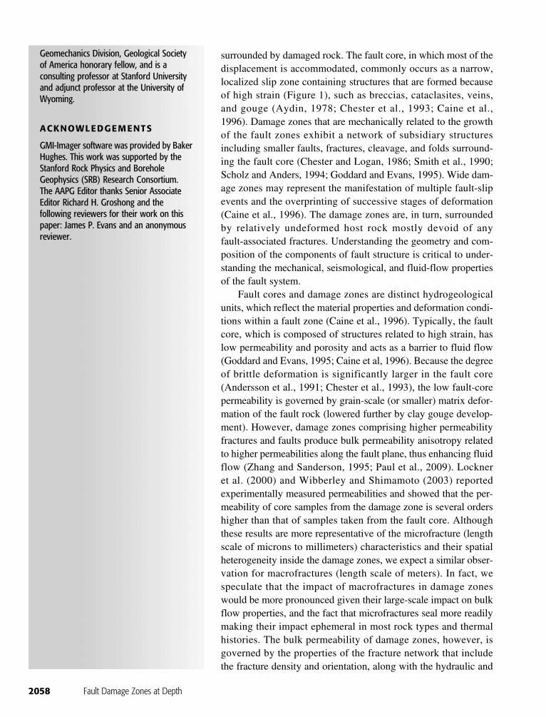
surrounded by damaged rock. The fault core, in which most of thedisplacement is accommodated, commonly occurs as a narrow,localized slip zone containing structures that are formed becauseof high strain (Figure 1), such as breccias, cataclasites, veins,and gouge (Aydin, 1978; Chester et al., 1993; Caine et al.,1996). Damage zones that are mechanically related to the growthof the fault zones exhibit a network of subsidiary structuresincluding smaller faults, fractures, cleavage, and folds surround-ing the fault core (Chester and Logan, 1986; Smith et al., 1990;Scholz and Anders, 1994; Goddard and Evans, 1995). Wide dam-age zones may represent the manifestation of multiple fault-slipevents and the overprinting of successive stages of deformation(Caine et al., 1996). The damage zones are, in turn, surroundedby relatively undeformed host rock mostly devoid of anyfault-associated fractures. Understanding the geometry and com-position of the components of fault structure is critical to under-standing the mechanical, seismological, and fluid-flow propertiesof the fault system.

Fault cores and damage zones are distinct hydrogeologicalunits, which reflect the material properties and deformation condi-tions within a fault zone (Caine et al., 1996). Typically, the faultcore, which is composed of structures related to high strain, haslow permeability and porosity and acts as a barrier to fluid flow(Goddard and Evans, 1995; Caine et al, 1996). Because the degreeof brittle deformation is significantly larger in the fault core(Andersson et al., 1991; Chester et al., 1993), the low fault-corepermeability is governed by grain-scale (or smaller) matrix defor-mation of the fault rock (lowered further by clay gouge develop-ment). However, damage zones comprising higher permeabilityfractures and faults produce bulk permeability anisotropy relatedto higher permeabilities along the fault plane, thus enhancing fluidflow (Zhang and Sanderson, 1995; Paul et al., 2009). Lockneret al. (2000) and Wibberley and Shimamoto (2003) reportedexperimentally measured permeabilities and showed that the per-meability of core samples from the damage zone is several ordershigher than that of samples taken from the fault core. Althoughthese results are more representative of the microfracture (lengthscale of microns to millimeters) characteristics and their spatialheterogeneity inside the damage zones, we expect a similar obser-vation for macrofractures (length scale of meters). In fact, wespeculate that the impact of macrofractures in damage zoneswould be more pronounced given their large-scale impact on bulkflow properties, and the fact that microfractures seal more readilymaking their impact ephemeral in most rock types and thermalhistories. The bulk permeability of damage zones, however, isgoverned by the properties of the fracture network that includethe fracture density and orientation, along with the hydraulic and

Geomechanics Division, Geological Societyof America honorary fellow, and is aconsulting professor at Stanford Universityand adjunct professor at the University ofWyoming.

ACKNOWLEDGEMENTS

GMI-Imager software was provided by BakerHughes. This work was supported by theStanford Rock Physics and BoreholeGeophysics (SRB) Research Consortium.The AAPG Editor thanks Senior AssociateEditor Richard H. Groshong and thefollowing reviewers for their work on thispaper: James P. Evans and an anonymousreviewer.

2058 Fault Damage Zones at Depth

mechanical characteristics of the fractures them-selves, and whether the fractures are sealed(Laubach, 2003; Olson et al., 2009).

The primary difficulty in predicting or modelingthe movement of hydrocarbons through damagezones arises because the permeability enhancementvaries significantly as a function of distance fromthe fault core as a result of the change in fracturedensity with distance. Thus, understanding the spa-tial variability of fracture density inside damagezones is one of the key aspects in evaluating theirimpact on flow. In addition, damage zones createspatial permeability anisotropy because of increasedflow paths (greater fracture density) and preferentialflow directions (along the fracture plane). In a frac-tured, low-matrix-permeability reservoir, fluiddrains from the fractures present in the surroundingrock mass into the highly permeable damage zoneswhere large flow rates can be maintained when the

well-perforation interval lies within the damagezone (Figure 1).

Several studies have documented the influence ofdamage zones on hydrocarbon production. Paul et al.(2009) studied a gas field in the Timor Sea where itwas only possible to explain large gas productionrates by introducing spatially variable permeabilityanisotropy associated with damage zones adjacent tofaults in the reservoir. Hennings et al. (2012) showedthat the wells that intersect damage zones, especiallythose with a large population of critically stressedfractures and faults in the Suban gas field (a fracturedgas reservoir with very low matrix permeability) inSoutheast Asia are most productive. Two wells withtrajectories that intersected the highest number offractures and faults in the damage zones of largerfaults showed an increase in well performance by fac-tors of 3 and 7 compared to wells not designed tointersect damage zones (Hennings et al., 2012).

Figure 1. A schematic of a fault zone showing the relatively impermeable fault core surrounded by the highly fractured damage zone.In a fractured, low matrix permeability reservoir, fluid from the fractures in the surrounding rock mass drains into the highly permeabledamage zones.

JOHRI ET AL. 2059

Despite their importance, the occurrence of per-meable fractures and small faults in damage zoneshave not traditionally been incorporated in reservoirsimulation models because of the inability of geolo-gists to provide damage-zone characteristics in aquantified manner that is practical to assimilate inflow-simulation models. In addition, the reluctanceof reservoir engineers to include more geologic com-plexity and associated uncertainty (regarding the spa-tial location, clustering, size, geometry, and flowproperties of fractures) contributed. However, we arebeginning to see this improve as a result of increasedcollaboration between the two communities (Pasalaet al, 2013; Zhang et al, 2013).

Flow-simulation models that do incorporate dam-age zones are usually generated by assigning effectivepermeability tensors to reservoir grid blocks. The per-meability tensor of each grid block depends on thecharacteristics of fractures inside the grid block, suchas fracture density, orientation, and fracture permeabil-ity. The outstanding question, therefore, is how do weestimate the spatial extent and heterogeneity of per-meability anisotropy at reservoir scale using the avail-able subsurface data? This issue can be addressed bystudying properties of damage zones, such as the spa-tial extent of damage zones and variation of fracturedensity with distance from the fault surface in damagezones using subsurface data such as image logs. Paulet al. (2009) adopted this methodology to study thedecay of fracture density inside damage zones.However, because all the wells in that study were out-side the fault-damage zones, they had no direct dataconstraint on damage-zone characteristics and the vari-ability of fracture density with distance from the fault.

We focus our attention on three primary damage-zone attributes: the spatial extent (width) of damagezones, the peak fracture density within damage zones,and the spatial heterogeneity of fracture densitywithin damage zones. These attributes are functionsof a wide range of factors, such as the amount of slipacross the fault, size of the fault (Mitchell andFaulkner, 2009), lithology, rupture processes, andmovement history (Caine et al., 1996). Variousoutcrop studies in the past have shown that fracturedensity inside damage zones decreases with distancefrom a fault (Schulz and Evans, 1998, 2000;Vermilye and Scholz, 1998; Shipton et al., 2005;

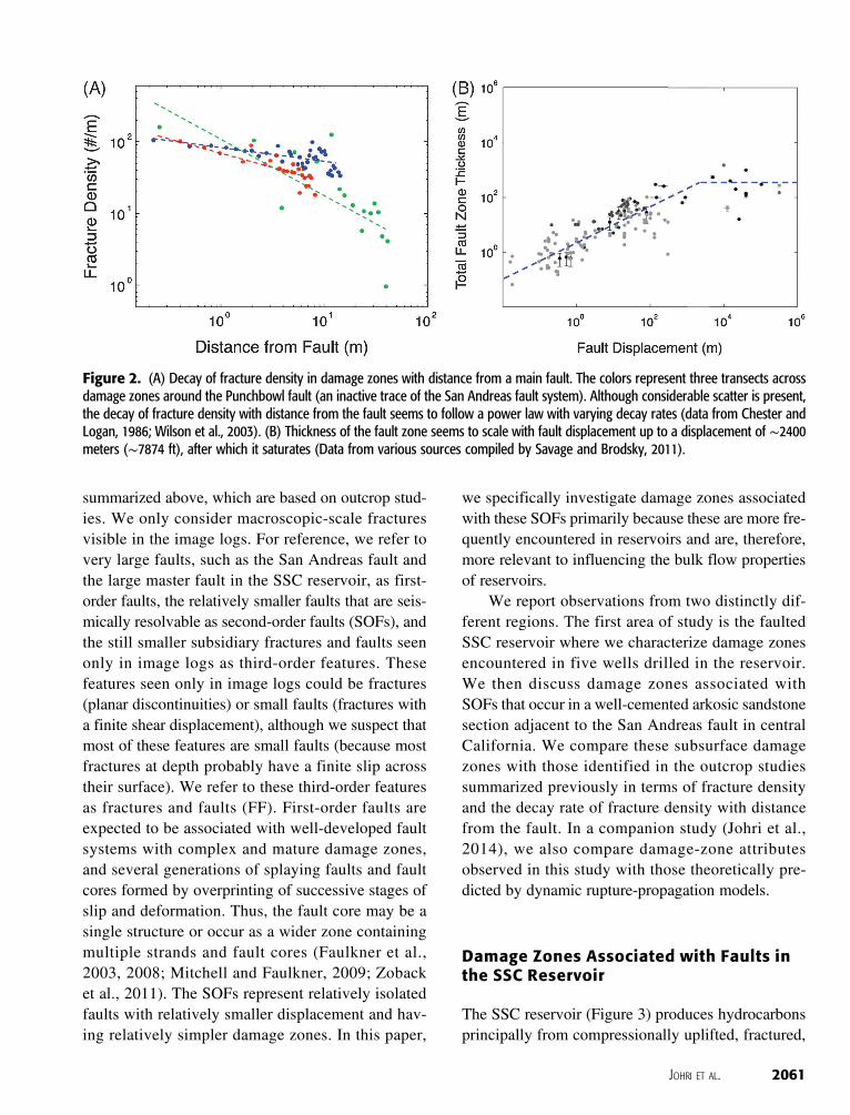
Mitchell and Faulkner, 2009; Savage and Brodsky,2011). Savage and Brodsky (2011) have suggestedthat the fracture density decays with distance fromisolated faults according to a power law F = F0r−n

in which F0 is the fault constant (the fracture densityat unit distance from the fault), r is the distance fromthe fault, and n is an exponent describing the decay(Figure 2A). Compiling various published fracture-density profiles, Savage and Brodsky (2011) find thedecay rate (n) is ∼0.8 for smaller faults (with slip lessthan ∼150 m [∼492 ft]), and it decreases for largerfaults with greater displacements. The authors alsoreport that the fault constant F0 is fault specific andseems to depend on lithology and fault displacement.However, an alternate study by Mitchell and Faulkner(2009) suggests that this fracture density at unit dis-tance is constant (∼100 fractures/m [30.5 fractures/ft]), independent of the size of the fault, and repre-sents a critical level of fracturing before fracture dam-age is so intense that brecciation and cataclasis begin.Previous studies have also reported that fracture-density decay can be expressed by exponential andlogarithmic laws (Chester et al., 2005; Faulkneret al, 2008). However, power law decay with distanceseems more reasonable because the stress perturba-tions, which eventually lead to damage, decay withthe inverse of distance from a propagating crack tipduring dynamic rupture propagation (Love, 1927;Freund, 1979). Several field studies and compilationshave also shown that damage zones grow linearlywith displacement, but not at all locations (Shiptonand Cowie, 2001), with most damage-zone growthoccurring early in the fault-slip history (Childs et al.,2009). Savage and Brodsky (2011) have reported thatthe fault zone width scales with cumulative fault dis-placement up to a threshold value of approximately2400 meters (7874 ft), beyond which the scalingbreaks down and further growth in the damage-zonewidth is more gradual (Figure 2B).

The presence and attributes of damage zones atdepth can be studied directly with ultrasonic andresistivity image logs, whereas sonic, resistivity, andporosity logs indicate changes in physical propertiesrelated to the presence of fractures. In this paper, wecharacterize subsurface damage zones at depth usingfault and fracture information derived from imagelogs, and then compare our observations with those

2060 Fault Damage Zones at Depth

summarized above, which are based on outcrop stud-ies. We only consider macroscopic-scale fracturesvisible in the image logs. For reference, we refer tovery large faults, such as the San Andreas fault andthe large master fault in the SSC reservoir, as first-order faults, the relatively smaller faults that are seis-mically resolvable as second-order faults (SOFs), andthe still smaller subsidiary fractures and faults seenonly in image logs as third-order features. Thesefeatures seen only in image logs could be fractures(planar discontinuities) or small faults (fractures witha finite shear displacement), although we suspect thatmost of these features are small faults (because mostfractures at depth probably have a finite slip acrosstheir surface). We refer to these third-order featuresas fractures and faults (FF). First-order faults areexpected to be associated with well-developed faultsystems with complex and mature damage zones,and several generations of splaying faults and faultcores formed by overprinting of successive stages ofslip and deformation. Thus, the fault core may be asingle structure or occur as a wider zone containingmultiple strands and fault cores (Faulkner et al.,2003, 2008; Mitchell and Faulkner, 2009; Zobacket al., 2011). The SOFs represent relatively isolatedfaults with relatively smaller displacement and hav-ing relatively simpler damage zones. In this paper,

we specifically investigate damage zones associatedwith these SOFs primarily because these are more fre-quently encountered in reservoirs and are, therefore,more relevant to influencing the bulk flow propertiesof reservoirs.

We report observations from two distinctly dif-ferent regions. The first area of study is the faultedSSC reservoir where we characterize damage zonesencountered in five wells drilled in the reservoir.We then discuss damage zones associated withSOFs that occur in a well-cemented arkosic sandstonesection adjacent to the San Andreas fault in centralCalifornia. We compare these subsurface damagezones with those identified in the outcrop studiessummarized previously in terms of fracture densityand the decay rate of fracture density with distancefrom the fault. In a companion study (Johri et al.,2014), we also compare damage-zone attributesobserved in this study with those theoretically pre-dicted by dynamic rupture-propagation models.

Damage Zones Associated with Faults inthe SSC Reservoir

The SSC reservoir (Figure 3) produces hydrocarbonsprincipally from compressionally uplifted, fractured,

Figure 2. (A) Decay of fracture density in damage zones with distance from a main fault. The colors represent three transects acrossdamage zones around the Punchbowl fault (an inactive trace of the San Andreas fault system). Although considerable scatter is present,the decay of fracture density with distance from the fault seems to follow a power law with varying decay rates (data from Chester andLogan, 1986; Wilson et al., 2003). (B) Thickness of the fault zone seems to scale with fault displacement up to a displacement of ∼2400meters (∼7874 ft), after which it saturates (Data from various sources compiled by Savage and Brodsky, 2011).

JOHRI ET AL. 2061

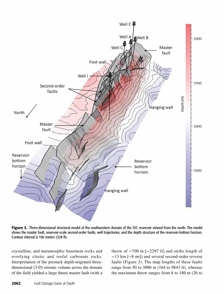
crystalline, and metamorphic basement rocks andoverlying clastic and reefal carbonate rocks.Interpretation of the prestack depth-migrated three-dimensional (3-D) seismic volume across the domainof the field yielded a large thrust master fault (with a

throw of ∼700 m [∼2297 ft] and strike length of∼13 km [∼8 mi]) and several second-order reversefaults (Figure 3). The map lengths of these faultsrange from 50 to 3000 m (164 to 9843 ft), whereasthe maximum throw ranges from 8 to 180 m (26 to

Figure 3. Three-dimensional structural model of the southwestern domain of the SSC reservoir viewed from the north. The modelshows the master fault, reservoir-scale second-order faults, well trajectories, and the depth structure of the reservoir-bottom horizon.Contour interval is 100 meters (328 ft).

2062 Fault Damage Zones at Depth

591 ft). All SOFs have a reverse separation. Theystrike subparallel to the master fault and are concen-trated in a 1×8 km (0.6×5 mi) area along the crestof the anticline. The region of interest is in the hang-ing wall of the master fault that is characterized by astrike-slip stress regime.

We examine five wells (Figure 3): A, B, C, E,and I. Wells A, E, and I are near-vertical wells, andwells B and C are deviated wells. Well tests sug-gested that poor correlation exists betweenwellbore–reservoir contact length and well perfor-mance, and also, a very weak correlation existsbetween well performance and the total number ofFF that the wells intersect. However, the well perfor-mance correlates strongly with the total number ofcritically stressed FF transected by the well.

According to the critically stressed-fault hypothe-sis, FF that are mechanically active are hydraulicallyconductive, and those that are mechanically dead arehydraulically dead (Barton et al., 1995; Zoback,2007). This means that faults on which the ratio ofresolved shear to effective normal stress is greaterthan the coefficient of sliding friction (normally about0.6; Byerlee, 1978) are expected to be mechanicallyactive and to slip. Fault slip may lead to dilatancyand brecciation (Dholakia et al., 1998), which in turnimparts enhanced permeability to the fracture.However, it is important to note that whereas the criti-cally stressed-fault hypothesis may help us identifywhich FF are likely to be permeable, and other geo-logic factors, such as degree of alteration and cemen-tation of the brecciated rock within the fracture, andits diagenetic history (Fisher and Knipe, 1998; Fisheret al., 2003), determine the actual permeability. Ofcourse, other viewpoints suggest that diagenesis maybe a critical factor that controls fracture permeability.For example, Laubach (2003) and Laubach et al.(2004) provide evidence that mechanically stable ordead fractures are not necessarily hydraulically deadand vice-versa. However, the critically stressedhypothesis appears to explain the hydraulic propertiesof fractures fairly well in the SSC reservoir.

Characterization of FF identified in image logs interms of local state of stress reveals that criticallystressed FF in the SSC reservoir are steeply dipping.Directing the well path through fault-damage zonesincreases the FF population that the well intersects,

whereas deviating them increases the probability ofwells intersecting a larger population of steeply dip-ping critically stressed FF. Wells B and C were pur-posely deviated to target fault-damage zones andhave potential well performance ranging from 3 to 7times higher than non-deviated wells.

Regions of anomalously high FF density (identi-fied in image logs) around SOFs encountered alongthe wells are interpreted as damage zones associatedwith those SOFs (Figure 4). The depths at which wellsintersect seismically interpreted SOFs are constrainedfrom seismic images whereas the positions of subseis-mic SOFs are constrained by identifying abruptchanges in bedding-plane orientations or concentra-tions in FF identified in image logs (in intervals wherebedding planes are absent or uninterpretable). For sub-seismic SOFs identified purely on the basis of regionalconcentrations in FF density, we observe a high FFdensity that decays sharply with distance on eitherside along the well—a significant damage-zonecharacter. The geomechanical modeling essential toconstraining the stress state and identifying criticallystressed FF is not reported here for proprietary rea-sons. The peak FF density and peak critically stressedFF density in most damage zones identified in thesewells is approximately 1.5–2 FF/m (0.5–0.6 FF/ft)and 0.25–0.5 FF/m (0.07–0.15 FF/ft), respectively(Figure 4). Many apparent damage zones appear tooverlap, making it difficult to identify their width.However, most damage zones appear to be approxi-mately 50–80 m (164–262 ft) wide (Figure 4). TheFF density is larger in the deviated well (well B) ascompared to the vertical wells. Most of the wells donot intersect the seismically identified SOFs. Well Aintersects only one of those faults (at 2490 m[8169 ft]), although we observe well-defined concen-trations of FF that resemble damage zones in imagelogs around positions marked by arrows in Figure 4.Well E does not intersect any seismically identifiedSOF, but it passes near one between 2700 and3100 m (8858 and 10171 ft). Thus, although it doesnot intersect the fault, it samples the damage zonealong an extended length. Several other well-defineddamage-zone-like features are observed around posi-tions marked by dotted blue arrows in well E(Figure 4), but direct evidence is lacking, suggestingthe presence of a fault. Well I is also not interpreted

JOHRI ET AL. 2063

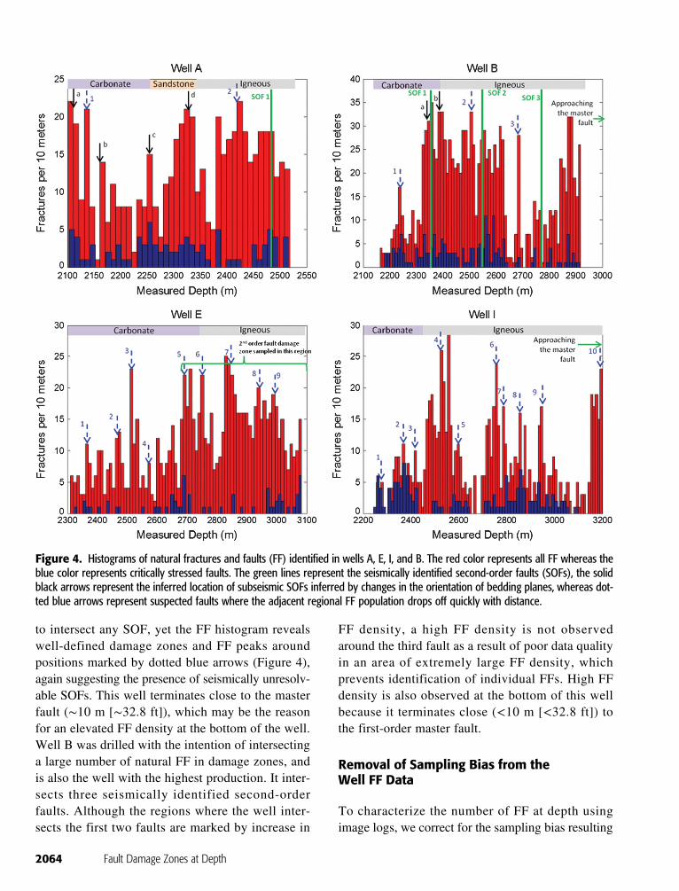
to intersect any SOF, yet the FF histogram revealswell-defined damage zones and FF peaks aroundpositions marked by dotted blue arrows (Figure 4),again suggesting the presence of seismically unresolv-able SOFs. This well terminates close to the masterfault (∼10 m [∼32.8 ft]), which may be the reasonfor an elevated FF density at the bottom of the well.Well B was drilled with the intention of intersectinga large number of natural FF in damage zones, andis also the well with the highest production. It inter-sects three seismically identified second-orderfaults. Although the regions where the well inter-sects the first two faults are marked by increase in

FF density, a high FF density is not observedaround the third fault as a result of poor data qualityin an area of extremely large FF density, whichprevents identification of individual FFs. High FFdensity is also observed at the bottom of this wellbecause it terminates close (<10 m [<32.8 ft]) tothe first-order master fault.

Removal of Sampling Bias from theWell FF Data

To characterize the number of FF at depth usingimage logs, we correct for the sampling bias resulting

Figure 4. Histograms of natural fractures and faults (FF) identified in wells A, E, I, and B. The red color represents all FF whereas theblue color represents critically stressed faults. The green lines represent the seismically identified second-order faults (SOFs), the solidblack arrows represent the inferred location of subseismic SOFs inferred by changes in the orientation of bedding planes, whereas dot-ted blue arrows represent suspected faults where the adjacent regional FF population drops off quickly with distance.

2064 Fault Damage Zones at Depth

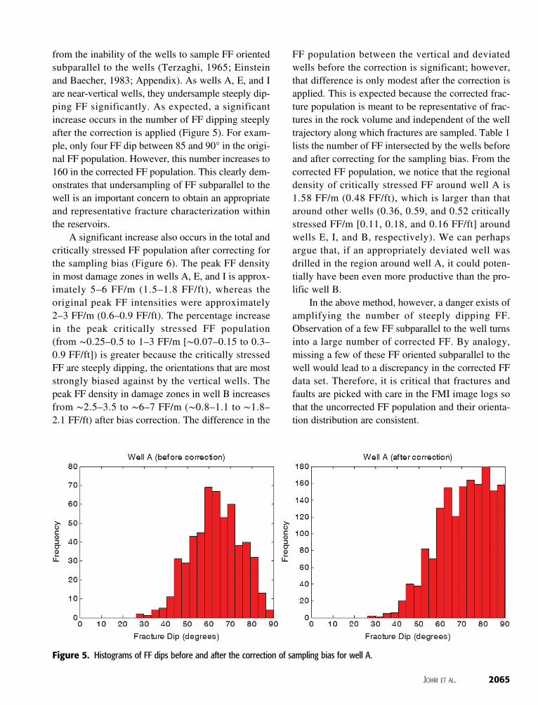
from the inability of the wells to sample FF orientedsubparallel to the wells (Terzaghi, 1965; Einsteinand Baecher, 1983; Appendix). As wells A, E, and Iare near-vertical wells, they undersample steeply dip-ping FF significantly. As expected, a significantincrease occurs in the number of FF dipping steeplyafter the correction is applied (Figure 5). For exam-ple, only four FF dip between 85 and 90° in the origi-nal FF population. However, this number increases to160 in the corrected FF population. This clearly dem-onstrates that undersampling of FF subparallel to thewell is an important concern to obtain an appropriateand representative fracture characterization withinthe reservoirs.

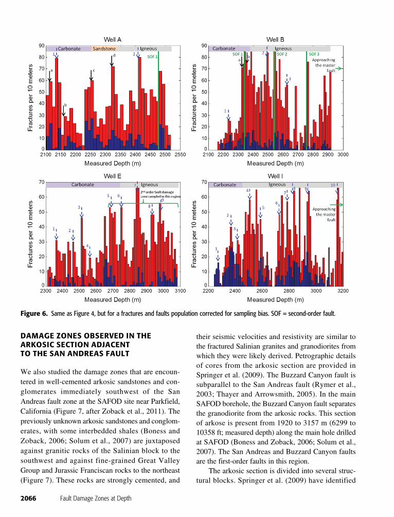
A significant increase also occurs in the total andcritically stressed FF population after correcting forthe sampling bias (Figure 6). The peak FF densityin most damage zones in wells A, E, and I is approx-imately 5–6 FF/m (1.5–1.8 FF/ft), whereas theoriginal peak FF intensities were approximately2–3 FF/m (0.6–0.9 FF/ft). The percentage increasein the peak critically stressed FF population(from ∼0.25–0.5 to 1–3 FF/m [∼0.07–0.15 to 0.3–0.9 FF/ft]) is greater because the critically stressedFF are steeply dipping, the orientations that are moststrongly biased against by the vertical wells. Thepeak FF density in damage zones in well B increasesfrom ∼2.5–3.5 to ∼6–7 FF/m (∼0.8–1.1 to ∼1.8–2.1 FF/ft) after bias correction. The difference in the

FF population between the vertical and deviatedwells before the correction is significant; however,that difference is only modest after the correction isapplied. This is expected because the corrected frac-ture population is meant to be representative of frac-tures in the rock volume and independent of the welltrajectory along which fractures are sampled. Table 1lists the number of FF intersected by the wells beforeand after correcting for the sampling bias. From thecorrected FF population, we notice that the regionaldensity of critically stressed FF around well A is1.58 FF/m (0.48 FF/ft), which is larger than thataround other wells (0.36, 0.59, and 0.52 criticallystressed FF/m [0.11, 0.18, and 0.16 FF/ft] aroundwells E, I, and B, respectively). We can perhapsargue that, if an appropriately deviated well wasdrilled in the region around well A, it could poten-tially have been even more productive than the pro-lific well B.

In the above method, however, a danger exists ofamplifying the number of steeply dipping FF.Observation of a few FF subparallel to the well turnsinto a large number of corrected FF. By analogy,missing a few of these FF oriented subparallel to thewell would lead to a discrepancy in the corrected FFdata set. Therefore, it is critical that fractures andfaults are picked with care in the FMI image logs sothat the uncorrected FF population and their orienta-tion distribution are consistent.

Figure 5. Histograms of FF dips before and after the correction of sampling bias for well A.

JOHRI ET AL. 2065

DAMAGE ZONES OBSERVED IN THEARKOSIC SECTION ADJACENTTO THE SAN ANDREAS FAULT

We also studied the damage zones that are encoun-tered in well-cemented arkosic sandstones and con-glomerates immediately southwest of the SanAndreas fault zone at the SAFOD site near Parkfield,California (Figure 7, after Zoback et al., 2011). Thepreviously unknown arkosic sandstones and conglom-erates, with some interbedded shales (Boness andZoback, 2006; Solum et al., 2007) are juxtaposedagainst granitic rocks of the Salinian block to thesouthwest and against fine-grained Great ValleyGroup and Jurassic Franciscan rocks to the northeast(Figure 7). These rocks are strongly cemented, and

their seismic velocities and resistivity are similar tothe fractured Salinian granites and granodiorites fromwhich they were likely derived. Petrographic detailsof cores from the arkosic section are provided inSpringer et al. (2009). The Buzzard Canyon fault issubparallel to the San Andreas fault (Rymer et al.,2003; Thayer and Arrowsmith, 2005). In the mainSAFOD borehole, the Buzzard Canyon fault separatesthe granodiorite from the arkosic rocks. This sectionof arkose is present from 1920 to 3157 m (6299 to10358 ft; measured depth) along the main hole drilledat SAFOD (Boness and Zoback, 2006; Solum et al.,2007). The San Andreas and Buzzard Canyon faultsare the first-order faults in this region.

The arkosic section is divided into several struc-tural blocks. Springer et al. (2009) have identified

Figure 6. Same as Figure 4, but for a fractures and faults population corrected for sampling bias. SOF = second-order fault.

2066 Fault Damage Zones at Depth

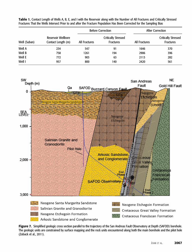
Table 1. Contact Length of Wells A, B, E, and I with the Reservoir along with the Number of All Fractures and Critically StressedFractures That the Wells Intersect Prior to and after the Fracture Population Has Been Corrected for the Sampling Bias

Well (Suban)Reservoir WellboreContact Length (m)

Before Correction After Correction

All FracturesCritically Stressed

Fractures All FracturesCritically Stressed

Fractures

Well A 234 547 91 1646 370Well B 758 1261 194 2906 396Well E 772 903 63 2113 282Well I 957 800 140 2420 561

Figure 7. Simplified geologic cross section parallel to the trajectory of the San Andreas Fault Observatory at Depth (SAFOD) borehole.The geologic units are constrained by surface mapping and the rock units encountered along both the main borehole and the pilot hole(Zoback et al., 2011).

JOHRI ET AL. 2067

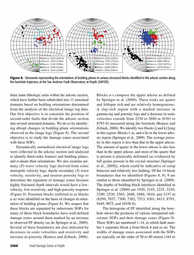
three main lithologic units within the arkosic section,which have further been subdivided into 11 structuraldomains based on bedding orientations determinedfrom the analysis of the electrical image log data.Our first objective is to constrain the position ofsecond-order faults that divide the arkosic sectioninto several structural domains. We do so by identify-ing abrupt changes in bedding-plane orientationsobserved in the image logs (Figure 8). The secondobjective is to study the damage zones associatedwith these SOFs.

Dynamically normalized electrical image logswere collected in the arkosic section and analyzedto identify third-order features and bedding planes,and evaluate their orientations. We also examine pri-mary (P) wave velocity logs derived from sonicmonopole velocity logs, dipole secondary (S) wavevelocity, resistivity, and neutron porosity logs todetermine the signature of damage zones becausehighly fractured depth intervals would have a low-velocity, low-resistivity, and high-porosity response(Figure 9). Fourteen blocks (referred to as blocksa–n) were identified on the basis of changes in orien-tation of bedding planes (Figure 8). We suspect thatthese blocks are separated by subseismic SOFs formany of these block boundaries have well-defineddamage zones around them marked by an increasein observed FF density (as do Springer et al., 2009).Several of these boundaries are also indicated bydecreases in sonic velocities and resistivity andincrease in porosity (Boness and Zoback, 2006).

Blocks a–i compose the upper arkose as definedby Springer et al. (2009). These rocks are quartzand feldspar rich and are relatively homogeneous.A clay-rich region with a marked increase ingamma-ray and porosity logs and a decrease in sonicvelocities extends from 2530 to 2680 m (8301 to8793 ft) measured along the borehole (Boness andZoback, 2006). We identify two blocks (j and k) lyingin this region. Blocks l, m, and n lie in the lower arko-sic region (Springer et al., 2009). The average poros-ity in this region is less than that in the upper arkose.The amount of quartz in the lower arkose is also lessthan in the upper arkose, and most of the quartz thatis present is plastically deformed (as evidenced byfull grains present in the crystal structure [Springeret al., 2009]), which could be indicative of creepbehavior and relatively less faulting. Of the 14 blockboundaries that we identified (Figures 8, 9), 9 aresimilar to those identified by Springer et al. (2009).The depths of bedding block interfaces identified inSpringer et al. (2009) are 1920, 2145, 2225, 2250,2290, 2530, 2565, 2680, 2880, 3010, and 3157 m(6299, 7037, 7300, 7382, 7513, 8301, 8415, 8793,9449, 9875, and 10358 ft).

The histogram of FF identified along the bore-hole shows the positions of various interpreted sub-seismic SOFs and their damage zones (Figure 9).These SOFs are numbered 1–14, in which fault num-ber 1 separates block a from block b and so on. Thewidths of damage zones associated with the SOFsare typically on the order of 50 to 80 meters (164 to

Figure 8. Stereonets representing the orientations of bedding planes in various structural blocks identified in the arkosic section alongthe borehole trajectory at the San Andreas Fault Observatory at Depth (SAFOD).

2068 Fault Damage Zones at Depth

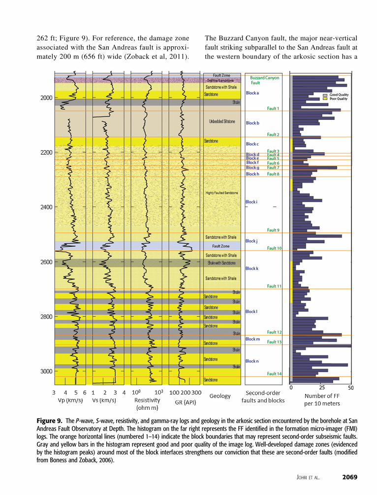
262 ft; Figure 9). For reference, the damage zoneassociated with the San Andreas fault is approxi-mately 200 m (656 ft) wide (Zoback et al, 2011).

The Buzzard Canyon fault, the major near-verticalfault striking subparallel to the San Andreas fault atthe western boundary of the arkosic section has a

Figure 9. The P-wave, S-wave, resistivity, and gamma-ray logs and geology in the arkosic section encountered by the borehole at SanAndreas Fault Observatory at Depth. The histogram on the far right represents the FF identified in the formation micro-imager (FMI)logs. The orange horizontal lines (numbered 1–14) indicate the block boundaries that may represent second-order subseismic faults.Gray and yellow bars in the histogram represent good and poor quality of the image log. Well-developed damage zones (evidencedby the histogram peaks) around most of the block interfaces strengthens our conviction that these are second-order faults (modifiedfrom Boness and Zoback, 2006).

JOHRI ET AL. 2069

damage zone ∼120 m (∼394 ft) in width (Figure 9).The width of damage zones associated with theSOFs are again interpreted as the interval along theborehole having a FF density larger than the back-ground FF density. Damage zones around faults 1,9, 12, and 14 are approximately 60–80 m (197–262 ft) wide, whereas those around faults 12 and 13appear to overlap each other. The peak FF densityaround these faults is approximately 3–4 FF/m(0.91–1.22 FF/ft). Damage zones around faults 3 to8 overlap each other. This may, perhaps, be a faultwith multiple strands. The peak FF density in theirdamage zone is approximately 2 FF/m (0.61 FF/ft).Damage zones around faults 2, 10, and 11 are fairlywell defined, but they have a relatively lower peakFF density. Poor image quality (probably caused byvery intense damage) could prevent identification ofdiscrete fractures. Damage zones around these faultsare approximately 40–50 meters (131–164 ft) wideand their peak FF density is approximately 1.5–2FF/m. We also observe a sharp decay in the densityof FF with distance from the fault. Several authorshave shown that the width of damage zones scaleswith slip across the fault (Mitchell and Faulkner,2009; Johri et al., 2014). If this is true, faults 1, 9,12, 13, and 14 may have a relatively greater slip.The P- and S-wave velocities, as expected, are usu-ally low in the vicinity of most suspected SOFs

(Figure 9). A marked decrease in velocities and resis-tivity occurs around SOFs numbered 1 and 10.However, damage-zone signatures around most ofthe other SOFs on the geophysical logs are onlysubtle, marked by a modest local decrease in veloc-ities and resistivity.

Removal of Sampling Bias from theSAFOD FF Data

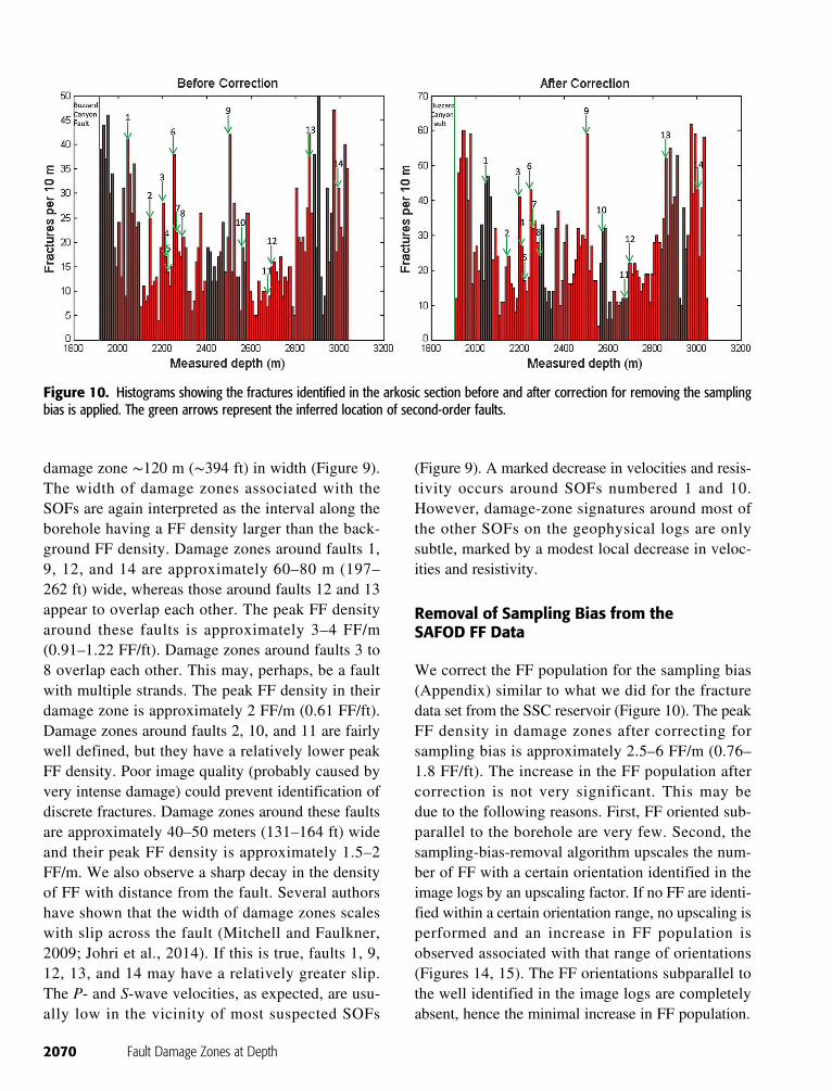
We correct the FF population for the sampling bias(Appendix) similar to what we did for the fracturedata set from the SSC reservoir (Figure 10). The peakFF density in damage zones after correcting forsampling bias is approximately 2.5–6 FF/m (0.76–1.8 FF/ft). The increase in the FF population aftercorrection is not very significant. This may bedue to the following reasons. First, FF oriented sub-parallel to the borehole are very few. Second, thesampling-bias-removal algorithm upscales the num-ber of FF with a certain orientation identified in theimage logs by an upscaling factor. If no FF are identi-fied within a certain orientation range, no upscaling isperformed and an increase in FF population isobserved associated with that range of orientations(Figures 14, 15). The FF orientations subparallel tothe well identified in the image logs are completelyabsent, hence the minimal increase in FF population.

Figure 10. Histograms showing the fractures identified in the arkosic section before and after correction for removing the samplingbias is applied. The green arrows represent the inferred location of second-order faults.

2070 Fault Damage Zones at Depth

VARIATION OF FF DENSITY WITH DISTANCEFROM FAULTS IN DAMAGE ZONES

We investigate the trend of decreasing FF densitywith distance from SOFs to compare them withobservations from outcrop studies. However, at leastthree inherent difficulties exist in performing thisanalysis using image logs. First, as the borehole inSAFOD and most wells in the SSC reservoir did notintersect seismically resolvable SOFs, the orientationof the SOFs is unknown. Thus, calculating theperpendicular distance of FF from the second-orderfault plane is difficult. Second, most damage zones

observed in the image logs overlap, so it is difficultto associate certain FF with a unique fault. Finally,varying image log quality at various intervals greatlyaffects the identifiable FF, and hence the damage-zone characteristics. These caveats should be kept inmind while drawing conclusions.

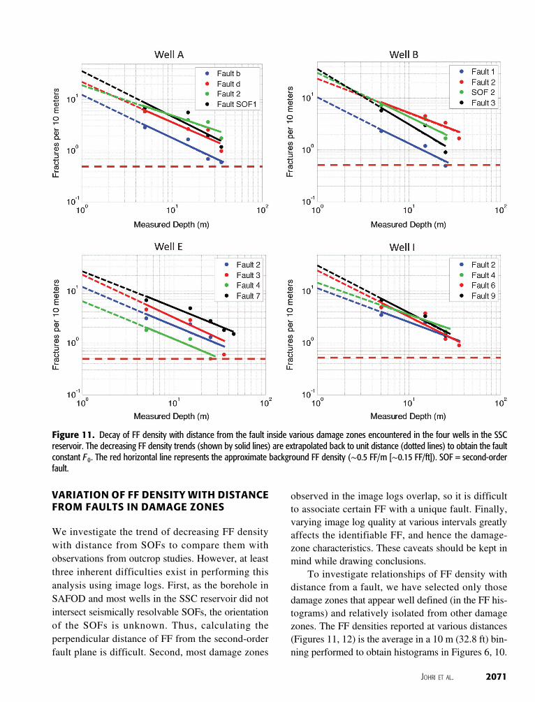
To investigate relationships of FF density withdistance from a fault, we have selected only thosedamage zones that appear well defined (in the FF his-tograms) and relatively isolated from other damagezones. The FF densities reported at various distances(Figures 11, 12) is the average in a 10 m (32.8 ft) bin-ning performed to obtain histograms in Figures 6, 10.

Figure 11. Decay of FF density with distance from the fault inside various damage zones encountered in the four wells in the SSCreservoir. The decreasing FF density trends (shown by solid lines) are extrapolated back to unit distance (dotted lines) to obtain the faultconstant F 0. The red horizontal line represents the approximate background FF density (∼0.5 FF/m [∼0.15 FF/ft]). SOF = second-orderfault.

JOHRI ET AL. 2071

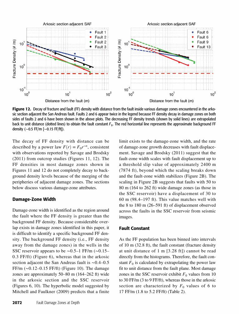
The decay of FF density with distance can bedescribed by a power law FðrÞ = F0r−n, consistentwith observations reported by Savage and Brodsky(2011) from outcrop studies (Figures 11, 12). TheFF densities in most damage zones shown inFigures 11 and 12 do not completely decay to back-ground density levels because of the merging of theperipheries of adjacent damage zones. The sectionsbelow discuss various damage-zone attributes.

Damage-Zone Width

Damage-zone width is identified as the region aroundthe fault where the FF density is greater than thebackground FF density. Because considerable over-lap exists in damage zones identified in this paper, itis difficult to identify a specific background FF den-sity. The background FF density (i.e., FF densityaway from the damage zones) in the wells in theSSC reservoir appears to be ∼0.5–1 FF/m (∼0.15–0.3 FF/ft) (Figure 6), whereas that in the arkosicsection adjacent the San Andreas fault is ∼0.4–0.5FF/m (∼0.12–0.15 FF/ft) (Figure 10). The damagezones are approximately 50–80 m (164–262 ft) widein the arkosic section and the SSC reservoir(Figures 6, 10). The hyperbolic model suggested byMitchell and Faulkner (2009) predicts that a finite

limit exists to the damage-zone width, and the rateof damage-zone growth decreases with fault displace-ment. Savage and Brodsky (2011) suggest that thefault-zone width scales with fault displacement up toa threshold slip value of approximately 2400 m(7874 ft), beyond which the scaling breaks downand the fault-zone width stabilizes (Figure 2B). Thescaling in Figure 2B suggests that faults with 50 to80 m (164 to 262 ft) wide damage zones (as those inthe SSC reservoir) have a displacement of 30 to60 m (98.4–197 ft). This value matches well withthe 8 to 180 m (26–591 ft) of displacement observedacross the faults in the SSC reservoir from seismicimages.

Fault Constant

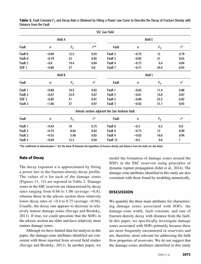
As the FF population has been binned into intervalsof 10 m (32.8 ft), the fault constant (fracture densityat unit distance of 1 m [3.28 ft]) cannot be readdirectly from the histograms. Therefore, the fault con-stant F0 is calculated by extrapolating the power lawfit to unit distance from the fault plane. Most damagezones in the SSC reservoir exhibit F0 values from 10to 30 FF/m (3 to 9 FF/ft), whereas those in the arkosicsection are characterized by F0 values of 6 to17 FF/m (1.8 to 5.2 FF/ft) (Table 2).

Figure 12. Decay of fracture and fault (FF) density with distance from the fault inside various damage zones encountered in the arko-sic section adjacent the San Andreas fault. Faults 2 and 6 appear twice in the legend because FF density decay in damage zones on bothsides of faults 2 and 6 have been shown in the above plots. The decreasing FF density trends (shown by solid lines) are extrapolatedback to unit distance (dotted lines) to obtain the fault constant F 0. The red horizontal line represents the approximate background FFdensity (∼0.5 FF/m [∼0.15 FF/ft]).

2072 Fault Damage Zones at Depth

Rate of Decay

The decay exponent n is approximated by fittinga power law to the fracture-density decay profile.The values of n for each of the damage zones(Figures 11, 12) are reported in Table 2. Damagezones in the SSC reservoir are characterized by decayrates ranging from 0.68 to 1.06 (average ∼0.8),whereas those in the arkosic section show relativelylower decay rates of ∼0.4 to 0.75 (average ∼0.56).Usually, the decay rate appears to decrease in rela-tively mature damage zones (Savage and Brodsky,2011). If true, we could speculate that the SOFs inthe arkosic section are older and have relatively moremature damage zones.

Although we have limited data for analysis in thispaper, the damage-zone attributes identified are con-sistent with those reported from several field studies(Savage and Brodsky, 2011). In another paper, we

model the formation of damage zones around theSOFs in the SSC reservoir using principles ofdynamic rupture propagation (Johri et al., 2014). Thedamage-zone attributes identified in this study are alsoconsistent with those found by modeling numerically.

DISCUSSION

We quantify the three main attributes for characteriz-ing damage zones associated with SOFs: thedamage-zone width, fault constant, and rate offracture-density decay with distance from the fault.In this paper, we specifically investigate damagezones associated with SOFs primarily because theseare more frequently encountered in reservoirs andare, therefore, more relevant for addressing the bulkflow properties of reservoirs. We do not suggest thatthe damage-zones attributes identified in this study

Table 2. Fault Constant F 0 and Decay Rate n Obtained by Fitting a Power Law Curve to Describe the Decay of Fracture Density withDistance from the Fault

SSC Gas Field

Well A Well E

Fault n F 0 r2* Fault n F 0 r2

Fault b −0.84 12.5 0.93 Fault 2 −0.75 12 0.79Fault d −0.79 22 0.85 Fault 3 −0.82 21 0.65Fault 2 −0.6 19.4 0.84 Fault 4 −0.73 6.4 0.84SOF 1 −0.89 37 0.8 Fault 7 −0.71 24.4 0.93

Well B Well I

Fault n F0 r2 Fault n F 0 r2

Fault 1 −0.89 10.5 0.92 Fault 1 −0.65 11.4 0.88Fault 2 −0.67 23.9 0.87 Fault 3 −0.61 14.6 0.87SOF 2 −0.85 31 0.91 Fault 5 −0.89 25.2 0.82Fault 3 −1.06 37 0.97 Fault 7 −0.92 31.7 0.93

Arkosic section adjacent the San Andreas fault

Fault n F0 r2 Fault n F 0 r2

Fault 1 −0.44 10 0.75 Fault 6 −0.3 6.3 0.9Fault 2 −0.74 8.64 0.82 Fault 6 −0.73 12 0.99Fault 2 −0.55 5.48 0.83 Fault 9 −0.63 16.6 0.94Fault 3 −0.69 12.5 0.94 Fault 13 −0.4 9.6 1

*The coefficients of determination r2 (for the linear fit between the logarithms of fracture density and distance from the fault) are also listed.

JOHRI ET AL. 2073

are exactly representative of all damage zones associ-ated with SOFs. These attributes may be a complexfunction of lithology, stress-state, regional tectonics,fault slip, and slip history, further complicated byoverprinting of multiple damage zones. Evidence alsoexists of asymmetric damage zones around undulatingfaults (Flodin and Aydin, 2004), which violate ourinference of a steady decay in FF density. However,we speculate that these attributes represent damagezones at a scale that affects the bulk flow propertiesand may be used as reasonable anchor pointswhile building reservoir models that include damagezones.

One of the shortcomings of this paper is the fail-ure to address the distribution of fracture length orsize within damage zones because we are limited pri-marily to image logs, which do not provide any infor-mation on the size of fractures. Image logs do providea size filter in terms of the minimum fracture cross-sectional response that can be resolved on the imagelog, but this is sensitive to whether the fracture is con-ducting or non-conducting. It is largely believed thatpower-law models describe the length distribution offractures. A large number of studies have beendevoted to analyzing the length distribution offractures (Segall and Pollard, 1983; Gudmundsson,1987; Villemin and Sunwoo, 1987; Childs et al.,1990; Scholz and Cowie, 1990; Davy, 1993; Odling,1997; Main et al., 1999) to test the power-law scalingmodel. However, despite numerous analyses andefforts, the statistical relevance of power-law modelsis not established among the scientific community,primarily due to difficulties in obtaining a robust stat-istical analysis on severely limited data sets(Pickering et al., 1995; Bonnet et al., 2001). In theabsence of a more established opinion and analysisin this study, we can perhaps speculate that power-law models can also describe the length distributionof FF within damage zones.

The quantified damage-zone attributes can helpincorporate the geometry and properties of damagezones in flow simulation models by assigning appro-priate effective permeability tensor values to variousreservoir grid blocks depending on fracture densityin those grid blocks, and the flow properties of thosefractures (Johri, 2012). For example, because thefracture-density decay with distance from the fault

can be described by a power law, the reservoir gridblocks close to the fault have larger permeability thatdecreases in grid blocks away from the fault surfacein accordance with the power-law decay relationship.We also notice that the damage-zone attributes inboth the SSC reservoir and arkosic sandstones arevery similar despite the difference in lithology. Thiscould suggest that damage-zone attributes in otherlithologies may be very similar, at least to first order.Such a result can be useful in the event of data scar-city. In the absence of image logs and other relevantfracture information, reasonable estimates of damagezones associated with reservoir-scale faults (the posi-tions of which are constrained from seismic images)can be made assuming their characteristics are similarto those identified in the current paper (Pasala et al,2013). Once the fracture network comprising fault-damage zones is modeled, fluid flow can be simu-lated by either upscaling fractures using effectivemedia modeling methods or directly using finite-element schemes for discrete fracture flow modeling(Dershowitz, 2000; Johri, 2012). Because simulatingflow through discrete fractures using finite-elementmethods is computationally expensive (especially ina dense fracture network typical of damage zones),the fracture population is usually upscaled to obtaineffective continuum grid flow properties using meth-ods, such as Oda’s method (Oda, 1985), and so on.Commercial simulators such as Eclipse can then beused for modeling flow. A methodology for includingdamage zones in building geologically representativereservoir discrete fracture network (DFN) models andmodeling flow through them is described in Johri(2012). Considering several realizations of damagezones using a range of values of fault constant anddecay rates can help perform uncertainty analysis inflow predictions.

We also demonstrate the importance of correctingthe FF population (obtained from image logs) for thesampling bias introduced caused by the undersam-pling of FF subparallel to the well. Significantincrease exists in the FF population, especially in theSSC reservoir in which the FF data set obtained fromimage logs is statistically corrected to remove the sam-pling bias. The corrected FF population representsthe number of FF that are expected to be present inthe rock mass, as opposed to the number observed in

2074 Fault Damage Zones at Depth

the image logs because of spatial sampling along aone-dimensional (1-D) linear well. The purpose of thisstatistical correction is to extrapolate a 3-D perspec-tive of the regional FF population from 1-D dataacquisition, and hence obtain a more meaningful frac-ture characterization. A well-constrained reservoirfracture characterization, along with knowledgeof prominent fracture sets, locations of SOFs, theirdamage-zone characteristics, and critically stressedFF orientations can help us design well trajectoriesthat could exploit damage zones and the more produc-tive critically stressed faults by orienting wellsperpendicular to them, in the process sampling mostof those FF and hence optimizing production. Aspreviously mentioned, it can also assist us in makingmore geologically informed reservoir models forsimulating fluid flow, and hence predicting productionrates and reservoir performance with greater accuracy.

CONCLUSIONS

We have identified the attributes of fault-damagezones associated with second-order faults (SOFs) atreservoir depths in two regions, the arkosic sectionadjacent to the San Andreas fault and the SSC reser-voirs. The SOFs and their damage zones are charac-terized using image and other geophysical logs. Thepositions of subseismic-resolution SOFs at depth areconstrained by noting changes in the orientation ofbedding planes and anomalous changes in geophysi-cal properties. Damage zones observed in both theregions are similar in terms of damage-zone widthsand fault constant F0 despite the geologic differences.These damage-zone characteristics are also very sim-ilar to those observed in outcrop studies. The decay offracture density with distance from faults can bedescribed by a power law F = F0r−n. Such a decayrate has been reported from outcrop field studies(Savage and Brodsky, 2011), and we have extendedit to damage zones at reservoir depths. The decay raten from 0.68 to 1.06 (average ∼0.8) is observed indamage zones in the SSC reservoir, whereas n from0.4 to 0.75 (average ∼0.56) is observed in damagezones in the arkosic sandstone section. Damage zonesin both the regions are typically 50–80 m (164–262 ft) wide. The extrapolated value of the faultconstant ranges from 10 to 30 FF/m (3 to 9 FF/ft)

for damage zones in the SSC reservoir and from 6 to17 FF/m (1.8 to 5.2 FF/ft) in those in the arkosic sec-tion. F0 for damage zones in the arkosic section mayhave been underestimated because of poor data qual-ity and intense fracturing.

APPENDIX: REMOVAL OF SAMPLING BIAS

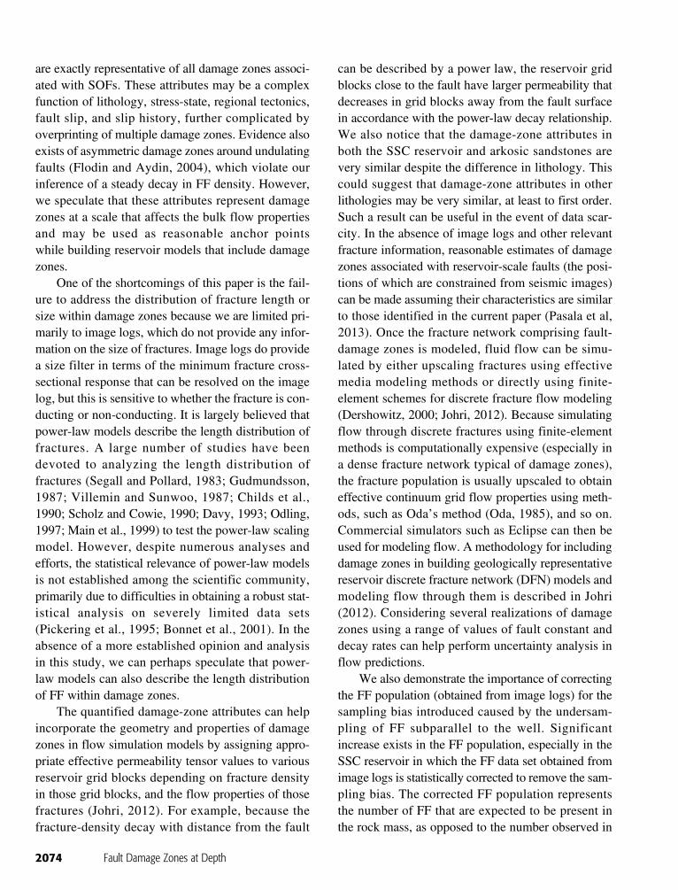
To characterize subsurface natural fractures and damage zonesusing geophysical logs such as image logs, it is necessary to cor-rect for the sampling bias introduced by the inability of wells tosample fractures oriented subparallel to them (Terzaghi, 1965;Einstein and Baecher, 1983). If we consider a set of fracturesintersecting a vertical well dipping at angle θ, and d is the actualaverage spacing between two fractures, the apparent fracturespacing as seen in the image log would be d∕ cos θ (Figure 13;Terzaghi, 1965). Consequently, if N is the number of fracturesintersecting this vertical well per unit length along the well, theactual fracture density of this fracture set would be N sec θ perunit length measured along the normal to this fracture set. Thisapproach can be extended to nonvertical wells (Figure 13). If weconsider a set of fractures striking α1 and dipping ϕ1, the trendand plunge of the normal to this fracture set would be ðα1 −90Þ° and ð90 − ϕ1Þ°. If the trend and plunge of the well are α2and ϕ2, then the unit vectors along the normal to the fracture set(u) and along the well (v) would be

~u = sinðα1 − 90Þ cosð90 − φ1Þ~ex+ cosðα1 − 90Þ cosð90 − φ1Þ~ey − sinð90 − φ1Þ~ez

~v = sinðα2Þ cosðφ2Þ~ex + cosðα2Þ cosðφ2Þ~ey − sinðφ2Þ~ez

Figure 13. Geometry of correction for the systematic under-sampling of steeply dipping fractures in a deviated well.

JOHRI ET AL. 2075

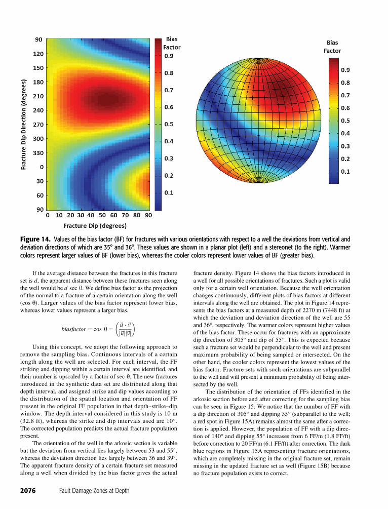
If the average distance between the fractures in this fractureset is d, the apparent distance between these fractures seen alongthe well would be d sec θ. We define bias factor as the projectionof the normal to a fracture of a certain orientation along the well(cos θ). Larger values of the bias factor represent lower bias,whereas lower values represent a larger bias.

biasfactor = cos  θ =�~u ·~vj~ujj~vj

�

Using this concept, we adopt the following approach toremove the sampling bias. Continuous intervals of a certainlength along the well are selected. For each interval, the FFstriking and dipping within a certain interval are identified, andtheir number is upscaled by a factor of sec θ. The new fracturesintroduced in the synthetic data set are distributed along thatdepth interval, and assigned strike and dip values according tothe distribution of the spatial location and orientation of FFpresent in the original FF population in that depth–strike–dipwindow. The depth interval considered in this study is 10 m(32.8 ft), whereas the strike and dip intervals used are 10°.The corrected population predicts the actual fracture populationpresent.

The orientation of the well in the arkosic section is variablebut the deviation from vertical lies largely between 53 and 55°,whereas the deviation direction lies largely between 36 and 39°.The apparent fracture density of a certain fracture set measuredalong a well when divided by the bias factor gives the actual

fracture density. Figure 14 shows the bias factors introduced ina well for all possible orientations of fractures. Such a plot is validonly for a certain well orientation. Because the well orientationchanges continuously, different plots of bias factors at differentintervals along the well are obtained. The plot in Figure 14 repre-sents the bias factors at a measured depth of 2270 m (7448 ft) atwhich the deviation and deviation direction of the well are 55and 36°, respectively. The warmer colors represent higher valuesof the bias factor. These occur for fractures with an approximatedip direction of 305° and dip of 55°. This is expected becausesuch a fracture set would be perpendicular to the well and presentmaximum probability of being sampled or intersected. On theother hand, the cooler colors represent the lowest values of thebias factor. Fracture sets with such orientations are subparallelto the well and will present a minimum probability of being inter-sected by the well.

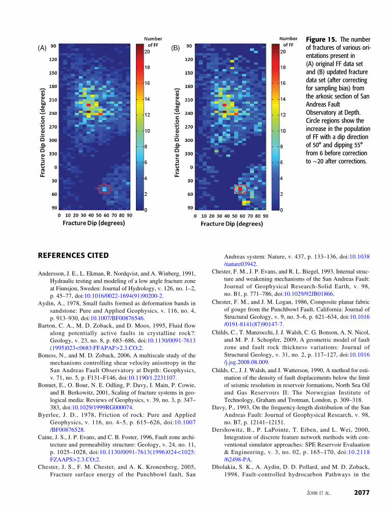
The distribution of the orientation of FFs identified in thearkosic section before and after correcting for the sampling biascan be seen in Figure 15. We notice that the number of FF witha dip direction of 305° and dipping 35° (subparallel to the well;a red spot in Figure 15A) remains almost the same after a correc-tion is applied. However, the population of FF with a dip direc-tion of 140° and dipping 55° increases from 6 FF/m (1.8 FF/ft)before correction to 20 FF/m (6.1 FF/ft) after correction. The darkblue regions in Figure 15A representing fracture orientations,which are completely missing in the original fracture set, remainmissing in the updated fracture set as well (Figure 15B) becauseno fracture population exists to correct.

Figure 14. Values of the bias factor (BF) for fractures with various orientations with respect to a well the deviations from vertical anddeviation directions of which are 35° and 36°. These values are shown in a planar plot (left) and a stereonet (to the right). Warmercolors represent larger values of BF (lower bias), whereas the cooler colors represent lower values of BF (greater bias).

2076 Fault Damage Zones at Depth

REFERENCES CITED

Andersson, J. E., L. Ekman, R. Nordqvist, and A. Winberg, 1991,Hydraulic testing and modeling of a low angle fracture zoneat Finnsjon, Sweden: Journal of Hydrology, v. 126, no. 1–2,p. 45–77, doi:10.1016/0022-1694(91)90200-2.

Aydin, A., 1978, Small faults formed as deformation bands insandstone: Pure and Applied Geophysics, v. 116, no. 4,p. 913–930, doi:10.1007/BF00876546.

Barton, C. A., M. D. Zoback, and D. Moos, 1995, Fluid flowalong potentially active faults in crystalline rock?:Geology, v. 23, no. 8, p. 683–686, doi:10.1130/0091-7613(1995)023<0683:FFAPAF>2.3.CO;2.

Boness, N., and M. D. Zoback, 2006, A multiscale study of themechanisms controlling shear velocity anisotropy in theSan Andreas Fault Observatory at Depth: Geophysics,v. 71, no. 5, p. F131–F146, doi:10.1190/1.2231107.

Bonnet, E., O. Bour, N. E. Odling, P. Davy, I. Main, P. Cowie,and B. Berkowitz, 2001, Scaling of fracture systems in geo-logical media: Reviews of Geophysics, v. 39, no. 3, p. 347–383, doi:10.1029/1999RG000074.

Byerlee, J. D., 1978, Friction of rock: Pure and AppliedGeophysics, v. 116, no. 4–5, p. 615–626, doi:10.1007/BF00876528.

Caine, J. S., J. P. Evans, and C. B. Foster, 1996, Fault zone archi-tecture and permeability structure: Geology, v. 24, no. 11,p. 1025–1028, doi:10.1130/0091-7613(1996)024<1025:FZAAPS>2.3.CO;2.

Chester, J. S., F. M. Chester, and A. K. Kronenberg, 2005,Fracture surface energy of the Punchbowl fault, San

Andreas system: Nature, v. 437, p. 133–136, doi:10.1038/nature03942.

Chester, F. M., J. P. Evans, and R. L. Biegel, 1993, Internal struc-ture and weakening mechanisms of the San Andreas Fault:Journal of Geophysical Research-Solid Earth, v. 98,no. B1, p. 771–786, doi:10.1029/92JB01866.

Chester, F. M., and J. M. Logan, 1986, Composite planar fabricof gouge from the Punchbowl Fault, California: Journal ofStructural Geology, v. 9, no. 5–6, p. 621–634, doi:10.1016/0191-8141(87)90147-7.

Childs, C., T. Manzocchi, J. J. Walsh, C. G. Bonson, A. N. Nicol,and M. P. J. Schopfer, 2009, A geometric model of faultzone and fault rock thickness variations: Journal ofStructural Geology, v. 31, no. 2, p. 117–127, doi:10.1016/j.jsg.2008.08.009.

Childs, C., J. J. Walsh, and J. Watterson, 1990, A method for esti-mation of the density of fault displacements below the limitof seismic resolution in reservoir formations, North Sea Oiland Gas Reservoirs II: The Norwegian Institute ofTechnology, Graham and Trotman, London, p. 309–318.

Davy, P., 1993, On the frequency-length distribution of the SanAndreas Fault: Journal of Geophysical Research, v. 98,no. B7, p. 12141–12151.

Dershowitz, B., P. LaPointe, T. Eiben, and L. Wei, 2000,Integration of discrete feature network methods with con-ventional simulator approaches: SPE Reservoir Evaluation& Engineering, v. 3, no. 02, p. 165–170, doi:10.2118/62498-PA.

Dholakia, S. K., A. Aydin, D. D. Pollard, and M. D. Zoback,1998, Fault-controlled hydrocarbon Pathways in the

Figure 15. The numberof fractures of various ori-entations present in(A) original FF data setand (B) updated fracturedata set (after correctingfor sampling bias) fromthe arkosic section of SanAndreas FaultObservatory at Depth.Circle regions show theincrease in the populationof FF with a dip directionof 50° and dipping 55°from 6 before correctionto ∼20 after corrections.

JOHRI ET AL. 2077

Monterey Formation, California: AAPG Bulletin, v. 82,no. 8, p. 1551–1574.

Einstein, H. H., and G. B. Baecher, 1983, Probabilistic and statis-tical methods in engineering geology specific methods andexamples, part 1: Exploration, Rock Mechanics andRock Engineering, v. 16, no. 1, p. 39–72, doi:10.1007/BF01030217.

Faulkner, D. R., A. C. Lewis, and E. H. Rutter, 2003, On theinternal structure and mechanics of large strike slip faultzones: Field observations of the Carboneras fault insoutheastern Spain: Tectonophysics, v. 367, no. 3–4,p. 235–251, doi:10.1016/S0040-1951(03)00134-3.

Faulkner, D. R., T. M. Mitchell, E. H. Rutter, and J. Cembrano,2008, On the structure and mechanical properties of largestrike slip faults, in C. A. J. Wibberley, W. Kurz, J. Imber,R. E. Holdsworth, and C. Collettini, eds., The InternalStructure of Fault Zones: Implications for Mechanical andFluid-Flow Properties: Geological Society, London:Special Publications, v. 299, p. 139–150, doi:10.1144/SP299.9.

Fisher, Q. J., and R. J. Knipe, 1998, Fault sealing processes insiliciclastic sediments, in G. Jones, Q. J. Fisher, and R. J.Knipe, eds., Faulting and Fault Sealing in HydrocarbonReservoirs: Geological Society, London, Special Publications,v. 147, p. 117–134, doi:10.1144/GSL.SP.1998.147.01.08.

Fisher, Q. J., M. Casey, S. D. Haris, and R. J. Knipe, 2003, Fluid-flow properties in sandstone: The importance of temperaturehistory: Geology, v. 3, no. 11, p. 965–1068, doi:10.1130/G19823.1.

Flodin, E., and A. Aydin, 2004, Faults with asymmetric damagezones in sandstone, Valley of Fire State Park, southernNevada: Journal of Structural Geology, v. 26, no. 5,p. 983–988, doi:10.1016/j.jsg.2003.07.009.

Freund, L. B., 1979, The mechanics of dynamic shear crackpropagation: Journal of Geophysical Research: Solid Earth(1978–2012), v. 84, no. B5, p. 2199–2209, doi:10.1029/JB084iB05p02199.

Gudmundsson, A., 1987, Geometry, formation, and developmentof tectonic fractures on the Reykjanes Peninsula, southwestIceland: Tectonophysics, v. 139, no. 3–4, p. 295–308,doi:10.1016/0040-1951(87)90103-X.

Goddard, J. V., and J. P. Evans, 1995, Chemical changes andfluid-rock interaction in faults of crystalline thrust sheets,northwestern Wyoming, U.S.A: Journal of StructuralGeology, v. 17, no. 4, p. 533–547, doi:10.1016/0191-8141(94)00068-B.

Hennings, P., P. Allwardt, P. Paul, C. Zahm, and R. Reid, 2012,Relationship between fractures, fault zones, stress and reser-voir productivity in the Suban gas field, Sumatra, Indonesia:AAPG Bulletin, v. 96, p. 753–772, doi:10.1306/08161109084.

Johri, M., 2012, Fault damage zones-observations, dynamic mod-eling, and implications on fluid flow: Ph.D. dissertation,Stanford University, 105–140 p.

Johri, M., E. M. Dunham, M. D. Zoback, and Z. Fang, 2014,Predicting fault damage zones by modeling dynamic rupturepropagation and comparison with field observations:Journal of Geophysical Research: Solid Earth, v. 119,no. 2, p. 1251–1272, doi:10.1002/2013JB010335.

Lockner, D., H. Naka, H. Tanaka, H. Ito, and R. Ikeda, 2000,Permeability and strength of core samples from the Nojimafault of the 1995 Kobe Earthquake: Proceedings of theInternational Workshop on the Nojima fault core and bore-hole data analysis, US Geol. Sur., p. 22–23.

Laubach, S. E., 2003, Practical approaches to identifying sealedand open fractures: AAPG Bulletin, v. 87, no. 4, p. 561–579.

Laubach, S. E., J. E. Olson, and J. F. W. Gale, 2004, Are openfractures necessarily aligned with maximum horizontalstress?: Earth & Planetary Science Letters, v. 222, no. 1,p. 191–195, doi:10.1016/j.epsl.2004.02.019.

Love, A. E. H., 1927, A Treatise on the Mathematical Theory ofElasticity, Cambridge University Press, Dover, New York,662 p.

Main, I. G., T. Leonard, O. Papasouliotis, C. G. Hatton, and P. G.Meredith, 1999, One slope or two? Detecting statisticallysignificant breaks of slope in geophysical data, with applica-tion to fracture scaling relationships: Geophysical ResearchLetters, v. 26, no. 18, p. 2801–2804.

Mitchell, T. M., and D. R. Faulkner, 2009, The nature and origin ofoff-fault damage surrounding strike-slip fault zones with awide range of displacements: A field study from the Atacamafault system, northern Chile: Journal of Structural Geology,v. 31, no. 8, p. 802–816, doi:10.1016/j.jsg.2009.05.002.

Oda, M., 1985, Permeability tensor for discontinuous rockmasses: Geotechnique, v. 35, no. 4, p. 483–495, doi:10.1680/geot.1985.35.4.483.

Odling, N. E., 1997, Scaling and connectivity of joint systems insandstones from western Norway: Journal of StructuralGeology, v. 19, no. 10, p. 1257–1271, doi:10.1016/S0191-8141(97)00041-2.

Olson, J. E., S. E. Laubach, and R. H. Lander, 2009, Natural frac-ture characterization in tight gas sandstones: Integratingmechanics and diagenesis: AAPG Bulletin, v. 93, no. 11,p. 1535–1549, doi:10.1306/08110909100.

Pasala, S. M., C. B. Forster, M. Deo, and J. P. Evans, 2013,Simulation of the impact of faults on CO2 injection intosandstone reservoirs: Geofluids, v. 13, no. 3, p. 344–358.

Paul, P., M. D. Zoback, and P. Hennings, 2009, Fluid flow in afractured reservoir using a geomechanically constrained faultzone damage model for reservoir simulation: SPE ReservoirEvaluation: Engineering, v. 12, no. 4, p. 562–575, doi:10.2118/110542-PA.

Pickering, G., J. M. Bull, and D. J. Sanderson, 1995, Samplingpower-law distributions: Tectonophysics, v. 248, no. 1,p. 1–20, doi:10.1016/0040-1951(95)00030-Q.

Rymer, M. J., R. D. Catchings, and M. R. Goldman, 2003,Structure of the San Andreas fault zone as revealed by sur-face geologic mapping and high-resolution seismic profilingnear Parkfield, California: Geophysical Research Abstracts,v. 5, p. 13,523.

Savage, H. M., and E. E. Brodsky, 2011, Collateral Damage:Evolution with displacement of fracture distribution and sec-ondary fault strands in fault damage zones: Journal ofGeophysical Research, v. 116, no. B3, 14 p, doi:10.1029/2010JB007665.

Scholz, C. H., and M. H. Anders, 1994, The permeability of faults,and the mechanical environment of fluids in faulting: U.S.Geological Survey Open-File Report 94-228, p. 247–253.

2078 Fault Damage Zones at Depth

Scholz, C. H., and P. A. Cowie, 1990, Determination of totalstrain from faulting using slip measurements: Nature,v. 346, p. 837–839, doi:10.1038/346837a0.

Schulz, S. E., and J. P. Evans, 1998, Spatial variability in micro-scopic deformation and composition of the Punchbowl fault,southern California: Implications for mechanisms, fluid–rock interaction, and fault morphology: Tectonophysics,v. 295, no. 1, p. 223–244.

Schulz, S. E., and J. P. Evans, 2000, Mesoscopic structure of thePunchbowl Fault, Southern California, and the geologic,and geophysical structure of active strike-slip faults:Journal of Structural Geology, v. 22, no. 7, p. 913–930.

Segall, P., and D. D. Pollard, 1983, Joint formation in granitic rockof the Sierra Nevada: Geological Society of America Bulletin,v. 94, no. 5, p. 563–575, doi:10.1130/0016-7606(1983).

Shipton, Z. K., and P. A. Cowie, 2001, Damage zone and slip-surface evolution over μm to km scales in high-porosityNavajo sandstone, Utah: Journal of Structural Geology,v. 23, no. 12, p. 1825–1844, doi:10.1016/S0191-8141(01)00035-9.

Shipton, Z. K., J. P. Evans, and L. B. Thompson, 2005, Thegeometry and thickness of deformation-band fault core andits influence on sealing characteristics of deformation-bandfault zones: AAPG memoir, v. 85, p. 181–195, doi:10.1306/1033723M853135.

Smith, L., C. B. Forster, and J. P. Evans, 1990, Interaction of faultzones, fluid flow, and heat transfer at the basin scale:Hydrogeology of permeability environments, in S. P.Newman and I. Neretnieks, eds., International Associationof Hydrogeological Sciences selected papers inHydrogeology, v. 2, p. 41–67.

Solum, J. G., S. Hickman, D. A. Lockner, S. Tembe, J. P. Evans,S. D. Draper, D. C. Barton, D. L. Kirschner, J. S. Chester,F. M. Chester, B. A. Van Der Pluijm, A. M. Schleicher,D. E. Moore, C. Moore, K. Bradbury, W. M. Calvin, andT. Wong, 2007, San Andreas fault zone mineralogy, geo-chemistry and physical properties from SAFOD cuttingsand core: Scientific Drilling Special Issue, v. 1, p. 64–67,doi:10.2204/iodp.sd.s01.34.2007.

Springer, D. S., J. Evans, J. I. Garver, D. Kirschner, and S. U.Janecke, 2009, Arkosic rocks from the San Andreas Faultobservatory at depth (SAFOD) borehole, central California:

Implications for the structure and tectonics of the SanAndreas Fault zone: Lithosphere, v. 1, no. 4, p. 206–226,doi:10.1130/L13.1.

Terzaghi, R. D. 1965, Sources of error in joint surveys:Geotechnique, v. 15, no. 3, p. 287–304.

Thayer, M., and R. Arrowsmith, 2005, Fault zone structure ofMiddle Mountain, central California: AmericanGeophysical Union, fall meeting, abstract T21A0458.

Vermilye, J. M., and C. H. Scholz, 1998, The process zone: Amicrostructural view of fault growth: Journal ofGeophysical Research, v. 103, no. B6, p. 12223–12237,doi:10.1029/98JB00957.

Villemin, T., and C. Sunwoo, 1987, Distribution logarithmiqueself-similaire des rejêts et longueurs de failles, exemple duBassin Houiller Lorrain: Compte Rendu, Acad. Sci. Paris,v. 305, p. 1309–1312 (in French).

Wibberley, A. J. C., and T. Shimamoto, 2003, Internal structureand permeability of major strike-slip fault zones: theMedian Tectonic Line in Mie Prefecture, Southwest Japan:Journal of Structural Geology, v. 25, p. 59–78, doi:10.1016/S0191-1814(02)00014-7.

Wilson, J. E., J. S. Chester, and F. M. Chester, 2003,Microfracture analysis of fault growth and wear processes,Punchbowl Fault, San Andreas system, California: Journalof Structural Geology, v. 25, no. 11, p. 1855–1873, doi:10.1016/S0191-8141(03)00036-1.

Zhang, Y., M. Person, J. Rupp, K. Ellett, M. A. Celia, C. W.Gable, and T. Elliot, 2013, Hydrogeologic controls oninduced seismicity in crystalline basement rocks due to fluidinjection into basal reservoirs: Groundwater, v. 51, no. 4,p. 525–538.

Zhang, X., and D. J. Sanderson, 1995, Anisotropic features ofgeometry and permeability in fractured rock masses:Engineering Geology, v. 40, no. 1–2, p. 65–75, doi:10.1016/0013-7952(95)00040-2.

Zoback, M. D. 2007, Reservoir Geomechanics: CambridgeUniversity Press, Cambridge, 341, 127–132 p.

Zoback, M. D., S. Hickman, and W. Ellsworth, 2011, Scientificdrilling into the San Andreas Fault Zone—An overview ofSAFOD’s first five years: Proceedings of the IntegratedOcean Drilling Program, v. 11, p. 14–28, doi:10.2204/iodp.sd.11.02.2011.

JOHRI ET AL. 2079