A Sampler of Graphs - Buffalo State College

A Sampler of GraphsBy Robin Sanders

In this notebook. we look at the shape of some important graphs. These are graphs that you should immediately know what kindof graph you'll get from the formula AND also you should know what kind of formula is likely to be involved from looking at apicture. This notebook is based on the material in Section 1.3 of the text.

Polynomials For a complete review of polynomial functions you should go through the material in Appendix D in the textbook. Polynomials come in two main flavors: Even degree polynomials and odd degree polynomials. If you zoom out far enough tosee the global behavior, all even degree polynomials eventually have the same basic shape. Likewise, if you zoom out farenough to see the global behavior, all odd degree polynomials eventually have the same basic shape.

ü Even degree polynomials

For example, let's compare the graph of f(x) = x2 to the graph of g(x) = x4 - 8 x3 - x2 + 68 x - 84. If we plot over a narrowrange of x values the pictures are quite different:

f1@x_D := x^2; g1@x_D := x^4 - 8 x^3 - x^2 + 68 x - 84;TableForm@88Plot@f1@xD, 8x, -5, 5<, PlotLabel Ø y == f1@xDD,

Plot@g1@xD, 8x, -5, 5<, PlotLabel Ø y == g1@xDD<<D

-4 -2 2 4

510152025y x2

-4 -2 2 4-100

100

200

300

y x4 - 8 x3 - x2 + 68 x - 84

But watch what happens when we zoom out---i.e. when we increase the range of x-values in the plot:

Manipulate@TableForm@88Plot@f1@xD, 8x, -a, a<, PlotLabel Ø y == f1@xDD,Plot@g1@xD, 8x, -a, a<, PlotLabel Ø y == g1@xDD<<D, 8a, 5, 50<D

a

-20 -10 10 20

100

200

300

400y x2

-20 -10 10 20

50000

100000

150000

200000

y x4 - 8 x3 - x2 + 68 x - 84

Except for the size of the y-values (and the flatness at the bottom of the U), this graph looks similar to the graph of y = x2. In factALL even degree polynomials with a POSITIVE leading coeffient eventually have a shape when you zoom out far enough.

Except for the size of the y-values (and the flatness at the bottom of the U), this graph looks similar to the graph of y = x2. In factALL even degree polynomials with a POSITIVE leading coeffient eventually have a shape when you zoom out far enough.

ü Odd degree polynomials

For example, let's compare the graph of f(x) = x3 to the graph of g(x) = x5 - 8 x4 - 91 x3 + 602 x2 + 1800 x - 5184. If we plot overa narrow range of x values the pictures are quite different:

f2@x_D := x^3; g2@x_D := x^5 - 8 x^4 - 91 x^3 + 602 x^2 + 1800 x - 5184TableForm@88Plot@f2@xD, 8x, -5, 5<, PlotLabel Ø y == f2@xDD,

Plot@g2@xD, 8x, -5, 5<, PlotLabel Ø y == g2@xDD<<D

-4 -2 2 4

-100

-50

50

100

y x3

-4 -2 2 4

-6000

-4000

-2000

2000

4000

y x5 - 8 x4 - 91 x3 + 602 x2 + 1800 x - 5184

But watch what happens when we zoom out---i.e. when we increase the range of x-values in the plot:

Manipulate@TableForm@88Plot@f2@xD, 8x, -a, a<, PlotLabel Ø y == f2@xDD,Plot@g2@xD, 8x, -a, a<, PlotLabel Ø y == g2@xDD<<D,

8a, 5, 50<, TableSpacing Ø 80, 10<D

a

22.4

-20 -10 10 20

-10000

-5000

5000

10000

y x3

-20 -10 10 20

-1.5µ106-1.µ106

-500000

500000

1.µ106

y x5 - 8 x4 - 91 x3 + 602 x2 + 1800 x - 5184

Except for the size of the y-values , this graph looks similar to the graph of y = x3. In fact ALL ODD degree polynomials with aPOSITIVE leading coefficient eventually have a shape if you zoom out far enough.

2 sampler-of-graphs-print-version.nb

ü Note about polynomials with NEGATIVE leading coefficients

If the leading coefficient of a polynomial is NEGATIVE, the global shaped is flipped over the x-axis. So we get TWOIMPORTANT FACTS:

If a polynomial has EVEN degree and a NEGATIVE leading coefficient, then it's global shape looks like

If a polynomial has ODD degree and a NEGATIVE leading coefficient, then it's global shape looks like

Rational functionsFor a complete review of rational functions you should go through the material in Appendix D in the textbook.

A rational function's symbolic formula is the ratio of two polynomials. In other words, if f HxLis a rational function, thenf HxL =

pHxLqHxL where pHxLand qHxLare polynomials.

The global shape of any RATIONAL FUNCTION is determined by nothing more than the dominant terms of its numerator anddenominator. Ignore all the lower order terms and just look at the ratio of the two dominant terms. The local behavior of thefunction depends on both the dominant terms and the lower order terms. As you saw in the first MAT163 lab, the roots of therational function and the roots of the polynomial in the numerator are typically the same; vertical asymptotes occur where thedenominator equals 0, and we get holes in the rational function at places where both the numerator and denominator equal 0.

ü Example 1: Predict the global behavior of f Hx L = x9+ 25 x3-17x6+ x5+x4+x3+x2+x+1.

. WRITE YOUR PREDICTION HERE:

WRITE YOUR ANSWER BEFORE TURNING THE PAGE!

sampler-of-graphs-print-version.nb 3

And now we check it out:

f3@x_D = Hx^9 + 25 x^3 - 17LêHx^6 + x^5 + x^4 + x^3 + x + 1L;Plot@f3@xD, 8x, -100, 100<D

-100 -50 50 100

-1.µ106

-500000

500000

1.µ106

Note that if we zoom in near 0, we will see some of the local behavior:

Plot@f3@xD, 8x, -5, 5<D

-4 -2 2 4

-200

-150

-100

-50

50

100

150

ü Example 2: Predict what happens to f Hx ) = 5 x5+ 24 x -192 x5-32

as x Æ ± •.WRITE YOUR PREDICTION HERE:

DO NOT TURN THE PAGE UNTIL YOU'VE WRITTEN DOWN YOUR PREDICTION ABOUT THE GLOBAL SHAPE


And now we check it out:

f4@x_D = H5 x^5 + 24 x - 19LêH2 x^5 - 32L;Plot@8f4@xD<, 8x, -100, 100<, PlotRange Ø AllD

-100 -50 50 100

-40

-20

20

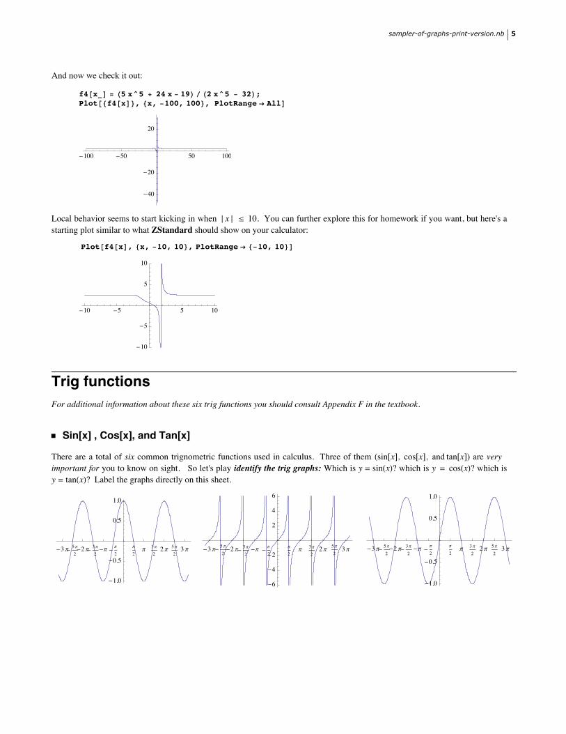
Local behavior seems to start kicking in when » x » § 10. You can further explore this for homework if you want, but here's astarting plot similar to what ZStandard should show on your calculator:

Plot@f4@xD, 8x, -10, 10<, PlotRange Ø 8-10, 10<D

-10 -5 5 10

-10

-5

5

10

Trig functionsFor additional information about these six trig functions you should consult Appendix F in the textbook.

ü Sin[x] , Cos[x], and Tan[x]

There are a total of six common trignometric functions used in calculus. Three of them Hsin@xD, cos@xD, and tan@xD) are veryimportant for you to know on sight. So let's play identify the trig graphs: Which is y = sinHxL? which is y = cosHxL? which isy = tanHxL? Label the graphs directly on this sheet.

-3 p- 5 p

2-2 p- 3 p

2-p -

p

2p

2p 3 p

22 p 5 p

23 p

-1.0

-0.5

0.5

1.0

-3 p- 5 p

2-2 p- 3 p

2-p -

p

2p

2p 3 p

22 p 5 p

23 p

-6

-4

-2

2

4

6

-3 p- 5 p

2-2 p- 3 p

2-p -

p

2p

2p 3 p

22 p 5 p

23 p

-1.0

-0.5

0.5

1.0


Now lets check our guesses:

TrigTicks = Table@Hk PiLê2, 8k, -100, 100<D;Plot@Sin@xD, 8x, -10, 10<, Ticks Ø 8TrigTicks, Automatic<, PlotLabel Ø y == Sin@xDD

-3 p- 5 p2-2 p- 3 p

2-p p

2p 3 p

22 p5 p

23 p

-1.0

-0.5

0.5

1.0y sinHxL

And now check your graph for Cos[x]:

Plot@Cos@xD, 8x, -10, 10<, Ticks Ø 8TrigTicks, Automatic<, PlotLabel Ø y ã Cos@xDD

-3 p- 5 p2-2 p- 3 p

2-p-

p

2p

2p 3 p

22 p5 p

23 p

-1.0

-0.5

0.5

1.0y cosHxL

PlotBTan@xD, 8x, -10, 10<, Ticks Ø 8TrigTicks, Automatic<, PlotLabel Ø "y = tanHxL =sin HxLcos HxL"F

-3 p- 5 p2-2 p- 3 p

2-p-

p

2p

2p 3 p

22 p 5 p

23 p

-6-4-2

246

y = tanHxL =sin HxLcos HxL

ü The other three trig functions

The other three trig functions are the reciprocals of the first (important) three trig functions. Secant is the reciprocal of the cosine. Here's a plot of y = secHxL = 1

cosHxL .

PlotBSec@xD, 8x, -10, 10<, Ticks Ø 8TrigTicks, Automatic<, PlotLabel Ø "y = secHxL =1

cos HxL"F

-3 p- 5 p2-2 p- 3 p

2-p-

p

2p

2p 3 p

22 p 5 p

23 p

-6-4-2

246

y = secHxL =1

cos HxL

The vertical asymptotes for secHxL occur when cosHxL = 0; the tops & bottoms of the U's have y = ±1and occur where cosHxL = ±1.

Cosecant is the reciprocal of the sine. Here's a plot of y = cscHxL = 1sinHxL .


Cosecant is the reciprocal of the sine. Here's a plot of y = cscHxL = 1sinHxL .

PlotBCsc@xD, 8x, -10, 10<, Ticks Ø 8TrigTicks, Automatic<, PlotLabel Ø "y = cscHxL =1

sin HxL"F

-3 p- 5 p2-2 p- 3 p

2-p-

p

2p

2p 3 p

22 p5 p

23 p

-5

5

y = cscHxL =1

sin HxL

The vertical asymptotes for cscHxL occur when sinHxL = 0; the tops & bottoms of the U's have y = ±1and occur where sinHxL = ±1.

Cotangent is the reciprocal of the tangent. Here's a plot of y = cotHxL = 1tanHxL = cosHxL

sinHxL .

PlotBCot@xD, 8x, -10, 10<, Ticks Ø 8TrigTicks, Automatic<,

PlotLabel Ø "y = cotHxL =1

tan HxL=cos HxLsin HxL"F

-3 p- 5 p2-2 p- 3 p

2-p-

p

2p

2p 3 p

22 p5 p

23 p

-6-4-2

246

y = cotHxL =1

tan HxL=cos HxLsin HxL

Note the vertical asymptotes for y = cotHxL occur where sinHxL = 0 and y = cotHxL crosses the x-axis when cosHxL = 0.

ü Putting all the Trig functions together: Here's are all six trig functions shown together.

-3 p- 5 p2-2 p- 3 p

2-p-

p

2p

2p 3 p

22 p 5 p

23 p

-1.0

-0.5

0.5

1.0y sinHxL

-3 p- 5 p

2-2 p- 3 p

2-p-

p

2p

2p 3 p

22 p 5 p

23 p

-1.0

-0.5

0.5

1.0y cosHxL

-3 p- 5 p2-2 p- 3 p

2-p-

p

2p

2p 3 p

22 p 5 p

23 p

-6

-4

-2

2

4

6

y = tanHxL = sin HxLcos HxL

-3 p- 5 p2-2 p- 3 p

2-p-

p

2p

2p 3 p

22 p 5 p

23 p

-5

5

y = cscHxL = 1sin HxL

-3 p- 5 p2-2 p- 3 p

2-p-

p

2p

2p 3 p

22 p 5 p

23 p

-6-4-2

246

y = secHxL = 1cos HxL

-3 p- 5 p2-2 p- 3 p

2-p-

p

2p

2p 3 p

22 p 5 p

23 p

-6-4-2

246

y = cotHxL = 1tan HxL

Exponential functions


Exponential functions

ü The graph of f Hx L = bx

The standard formula for a basic exponential function is f HxL = bx. What's it look like if b > 1? Draw your guess here:

DO NOT TURN THE PAGE UNTIL YOU'VE DRAWN YOUR GUESS!


And let's now check if you're correct:

b = 2; Plot@b^x, 8x, -5, 5<, PlotRange Ø 8-1, 20<, PlotLabel Ø y ã bxD

-4 -2 2 4

5

10

15

20y 2x

Now let's play with what happens to the graph as we change the value of b:

Manipulate@Plot@b^x, 8x, -5, 5<, PlotRange Ø 8-1, 20<, PlotLabel Ø y ã b^xD, 88b, 2<, 1ê10, 10<D

b

7.8418

-4 -2 2 4

5

10

15

20y 7.8418x

Your observations about all exponential graphs: (FILL IN THE BLANKS BEFORE YOU TURN THE PAGE)

1) All the y = bx graphs go through the point ___________________________________________________________

2) When b > 1, the graph of y = bx is ___________________________________________________________________

and we have an ________________________ asymptote at _______________________________________________________

3) When b = 1, the graph of y = bx is __________________________________________________________________

4) When 0 < b < 1, the graph of y = bx is ______________________________________________________________


Our class observations about all exponential graphs: (These are the answers to the FILL IN THE BLANKS on the previous page.)


Our class observations about all exponential graphs: (These are the answers to the FILL IN THE BLANKS on the previous page.)

1) All the y = bx graphs go through the point (1, 0) because b0 = 1 for all values of b.

2) When b > 1, the graph of y = bx is increasing and concave up. Also notice that as x Æ -•, bx Æ 0. So we also have a one-sided horizontal asymptote at x = 0.

3) When b = 1, the graph of y = bx is the horizontal line y = 1.

4) When 0 < b < 1, the graph of y = bx is decreasing and concave up. Also notice that as x Æ +•, bx Æ 0. So we also have a one-sided horizontal asymptote at x = 0.

ü The graph of f Hx L = b-x

An important variation on the theme of exponential functions are exponential functions with negative exponents. What's theshape of y = b-x look like? Draw what you think y = e-x looks like here:

DO NOT TURN THE PAGE UNTIL YOU'VE DRAWN YOUR GUESS!


Now let's check:

Manipulate@Plot@b^H-xL, 8x, -5, 5<, PlotRange Ø 8-1, 20<, PlotLabel Ø y ã b^H-xLD, 88b, 2<, 1ê10, 10<D

b

3.4264

-4 -2 2 4

5

10

15

20y 3.4264-x

Your observations about all exponential graphs with negative exponents: (FILL IN THE BLANKS BEFORE YOU TURN THE PAGE)

1) All the y = bx graphs go through the point ___________________________________________________________

2) When b > 1, the graph of y = bx is ___________________________________________________________________


3) When b = 1, the graph of y = bx is __________________________________________________________________

4) When 0 < b < 1, the graph of y = bx is ______________________________________________________________



Our class observations about all exponential graphs with negative exponents: (These are the answers to the FILL IN THE BLANKS on the previous page.

1) All the y = b-x graphs go through the point (1, 0) because b0 = 1 for all values of b.

2) When b > 1, the graph of y = b-x is decreasing and concave up. Also notice that as x Æ •, bx Æ 0. So we also have a one-sided horizontal asymptote at x = 0.

3) When b = 1, the graph of y = b-x is the horizontal line y = 1.

4) When 0 < b < 1, the graph of y = bx is increasing and concave up. Also notice that as x Æ -•, bx Æ 0. So we also have a one-sided horizontal asymptote at x = 0.

ü TWO important connections concerning exponential graphs

ü CONNCTION 1: What's the connection between the graph of y = b-x and the graph y = H1 êbLx? Fill in your prediction here:

DO NOT TURN THE PAGE UNTIL YOU'VE MADE YOUR PREDICTION!


Here are the plots:

Manipulate@Plot@8b^H-xL, H1êbL^x<, 8x, -5, 5<, PlotRange Ø 8-1, 20<D, 88b, 2<, 1ê10, 10<D

b

3.07

-4 -2 2 4

5

10

15

20

We're only getting one graph here! Can you explain why? Use the space below.Hint: Use exponent rules in your explanation.

DO NOT TURN THE PAGE UNTIL YOU'VE TRIED TO ANSWER THE QUESTION!

Recall that b-x means to take the reciprocal of bx. In other words,


Recall that b-x means to take the reciprocal of bx. In other words,

y = b-x = 1 ê HbxL = H1 ê bLx

by standard exponent rules. So of course y = b-x and y = H1 ê bLx give us the same graph.

† CONNCETION 2: What's the connection between the graph of y = b-x and the graph y = bx? Fill in your prediction here:

DO NOT TURN THE PAGE UNTIL YOU'VE MADE YOUR PREDICTION!


Here are the plots:

Manipulate@Plot@8b^x, b^H-xL<, 8x, -5, 5<, PlotRange Ø 8-1, 20<D, 88b, 2<, 1ê10, 10<D

b

3.4264

-4 -2 2 4

5

10

15

20

The graphs are mirror images across the y-axis! Can you explain why? Use the space below.HINT: Do you remember any connection between the graph of y = f HxL and the graph of y = f H-xL?

DO NOT TURN THE PAGE UNTIL YOU'VE TRIED TO ANSWER THE QUESTION!


SHORT EXPLAINATION: Note that if we let f HxL = bx then f H-xL = bx. The graphs of y = f HxL and y = f H-xL are alwaysreflections across the y-axis. You might rember learning this fact back in pre-calculus.

LONGER EXPLAINATION: This full explanation was probably covered in your pre-calculus course: We start by letting Ha, bL denote a point on the curve y = f HxL. That means that we know f HaL = b. The reflection of Ha, bLacross the y-axis is the point H-a, bL. And we now examine why H-a, bL must lie on the curve y = f H-xL. First recall that anypoint on y = f H-xL has coordinates of the form: Hx, f H-xLL. So H-a, bL lies on y = f H-xL if and only if b equals the value off H-H-aLL. But we already know f H-H-aLL = f HaL = b since Ha, bL lies on y = f HxL.

Logarithmic functions

ü The natural logarithm: y = lnHx L (done)

The only logarithm function that will be critically important to us is the natural log, and we'll study the formal (symbolic)properties of the natural logarithm function in some depth later in the semester. Here's a very good picture of y = lnHxL: In[30]:= Plot@Log@xD, 8x, 0, 10<, PlotRange Ø 8-3, 2.5<, PlotLabel Ø "y = lnHxL"D

Out[30]= 2 4 6 8 10

-3

-2

-1

1

2

y = lnHxL

Mathematica TIP: Mathematica uses the syntax Log[x] to denote lnHxL. (It's base is e º 2.71828.)

Your observations about lnHxL: (FILL IN THE BLANKS BEFORE YOU TURN THE PAGE)

1) The DOMAIN of lnHxL is _____________________________________________________________________

2) As x Ø 0 from the RIGHT (positive) side, we see lnHxL Ø___________________________________________

And there is a ________________________ asymptote for y = lnHxL at _________________________________

3) As x Ø +¶, we see lnHxL Ø ___________________________________________________________________

4) The graph y = lnHxL passes through the point ______________________________________________________

5) The graph y = ln(x) looks like _________________________________________________________________

Class Observations about y = lnHxL:(These are the answers to the fill in the blank questions on the previous page.)


Class Observations about y = lnHxL:(These are the answers to the fill in the blank questions on the previous page.)

1) The DOMAIN of lnHxL is the set of POSITIVE NUMBERS. So ln(-5) is NOT defined.

2) As x Ø 0 from the RIGHT (positive) side, we see lnHxL Ø -• very, very quickly. [So there is a VERTICAL asymptote for y = lnHxL at x = 0.]

3) As x Ø +¶, we see lnHxL Ø +• very, very slowly. [So there is not a horizontal asymptote for y = lnHxL.] 4) The graph y = lnHxL passes through the point (1, 0)

5) The graph y = ln(x) looks like an exponential function on its side!

In fact, as the next true scale plot shows, the graphs of y = lnHxL and y = ex are reflections of each other across the line y = x:

Plot@8Log@xD, x, E^x<, 8x, -3, 4<, PlotRange Ø 8-3, 4<, AspectRatio Ø AutomaticD

-3 -2 -1 1 2 3 4

-3

-2

-1

1

2

3

4


ü Other logarithms

You may recall from pre-calculus that there is a whole family of logarithm functions where we use logbHxLto denote the ``log-base-b '' function. If we have time, we may study the formal properties of these functions in a bit more detail later in the course, Fornow it' s enough to realize that logs are exponential functions on their sides! Hence they all have the same basic shape:

ManipulateAPlotALog@b, xD, 8x, 0, 20<, PlotRange Ø 8-10, 5<,PlotLabel Ø TableFormA99"y = log"b, "HxL"==, TableSpacing Ø 80, 0<EE, 88b, E<, 1ê10, 10<E

b

3.7828

5 10 15 20

-10

-8

-6

-4

-2

2

4

y = log3.7828HxL

Observations:

1) All logs with b > 1 have the same basic shape as lnHxL. As b Ø +¶, the graph of y = logbHxL becomes even flatter--- i.e. it takes even longer for the value of logbHxL to become large.

2) Logs with 0 < b < 1 are reflections (across the x-axis) of log curves with base H1 ê bL > 1.

3) ALL LOGS pass through the point (1, 0).

Mathematica TIP: Mathematica uses the syntax Log[b, x] to denote logbHxL, the so-called ``log-base-b'' function (So Log[b, x] = logbHxL in regular notation.)

Mathematics TIP: The base of a log function cannot equal 1. In other words, the symbol string log1HxL is MEANINGLESS in mathematics


Documents

A Sampler of Graphs - Buffalo State College