“A first approach to a Simultaneous Localisation

and Mapping (SLAM) solution implementing the

Extended Kalman Filter for visual odometry

data”

Juan Andres Carvajal

August 29, 2014

Abstract

This project was a done as a final grade project to obtain the degree in com-munications electronics engineering from TECNUN. It was done at Vicomtechunder the supervision of Leonardo de Maeztu , Marcos Nieto and Ainhoa Cortes.This project has consisted on the study and a fist approach implementation ofa simultaneous localisation and mapping algorithm. The algorithm of choicewas the EKF SLAM(Extended Kalman Filter Simultaneous Localisation andMapping).To properly understand the concepts behind SLAM and its imple-mentation various papers and project reports have been read, but the theoret-ical implementation and the practical implementation have been mostly basedon the report by Jose-Luis Blanco,“Derivation and Implementation of a Full6D EKF-based Solution to Bearing-Range SLAM”[9]. Also for the implemen-tation , the software C++ has been used with the help of the OpenCV libraryfor the handling and processing of images and matrices. Matlab was also usedwhen complicated math operations needed to be done. The implementationswas made with the help of previous code provided by Vicomtech [1] . The codeprovided contained a successful implementation of a visual odometry problemand it included most of the image processing needed for the next steps of thisproject.

1

Chapter 1

Introduction

1.1 The SLAM Problem

When we talk about SLAM (Simultaneous Localisation and Mapping) we shouldnot think of SLAM as only an algorithm but we should think of it as more of a“concept”[3].In SLAM we imagine a robot, or any type of mobile agent for thatmatter (e.g., a car), placed in an environment unknown to him. To properlysolve the SLAM problem this robot should be able to incrementally build amap of the environment it is in (mapping) and at the same time it should locatehimself within this map(localisation)[2]with the help of sensors incorporated toit. We could say we call it more a concept than just an algorithm because it isa specific situation in which we have a problem and it can be solved in manydifferent ways, and depending on the environment the best solution possiblecould vary.

The birth of SLAM could be tracked to the 1986 IEEE Robotics and Au-tomation Conference held in San Francisco, California. There many researchersincluding Peter Cheeseman, Jim Crowley, and Hugh Durrant- Whyte recognisedthat consistent probabilistic mapping was a fundamental problem in robotics [2].Over the next years a lot of research was done in this subject and many inter-esting findings and papers were published. Among the most important oneswere the ones by Smith et al which showed that as a robot moves through theenvironment taking observations of landmarks relative to the robot in the map,these estimated landmarks will all be correlated with each other because of thecommon error in the estimated vehicle position[4][5]. This implied that to solvethe full SLAM problem we needed a state vector formed of both the position ofthe robot and all of the observations, and both of these would have to be updatedevery time we had a new observation. This state vector could be huge and theproposed solution could be very complex and costly, computationally speaking.Because of this and because of the believe that the estimated map errors wouldnot converge and that the estimated error would grow in an unbounded mannerresearchers tried to minimise or eliminate the correlation between landmarks,

2

and research focused on solving the problem treating mapping and localisationseparately [2].

The key to SLAM as we know it today was when it was realised that theproblem was actually convergent and the correlations between landmarks werevital to the solution of the problem, and the bigger the correlation the betterthe solution would be[2]. At the International Symposium on Robotics Re-search (ISRR’99) in 1999 the Kalman filter based SLAM and its achievementsby Sebastian Thrun were presented and discussed[6].

1.2 Structure of the SLAM Problem

To understand the proposed solution we need to identify the agents involved inSLAM, their notations and their actions.

We, of course, have the mobile agent which moves around in the environment.We will denote the position of the robot at time k as xk. Consequently theposition of the robot at time k-1 will be denoted xk−1 ,and so on. The controlvector uk takes the agent from position xk to xk+1. We will call this transitionthe motion model.

As the agent moves it will discover interesting features through its sensors.The information of the position of the feature the sensors gives us which isrelative to the position at time k of the agent will be called observation. Wewill denote the different observations as zi,k. Meaning that it is the observationof feature i at time k.When we have this two options can follow:

The first option is that the feature i has never been seen before.When thishappens we will obtain the position of this feature relative to the point (0,0) ofour coordinate system( absolute position) using a model called inverse obser-vation model. When we have it described as an absolute position we will callit a landmark, which we will denote as mi.Landmarks are the ones which willdescribe our environment or as we called it earlier, our map. The location ofthese landmarks and the position of the robot mentioned previously will all havea level of uncertainty because of errors in the sensors and noise. This leads usto our second option.

The other option is that the observed feature has already been seen before,and that means it is already a landmark in our map. We use this to correct boththe position of the moving agent and the position of the landmarks. The way ofdoing this is by trying to predict the value of the observation using the positionof the corresponding landmark and the position of the robot. This process ofpredicting the value will be the direct observation model.

The motion model,the inverse observation model,and the direct observationmodel and how we apply them specifically in our system will all be explainedlater on this report.

3

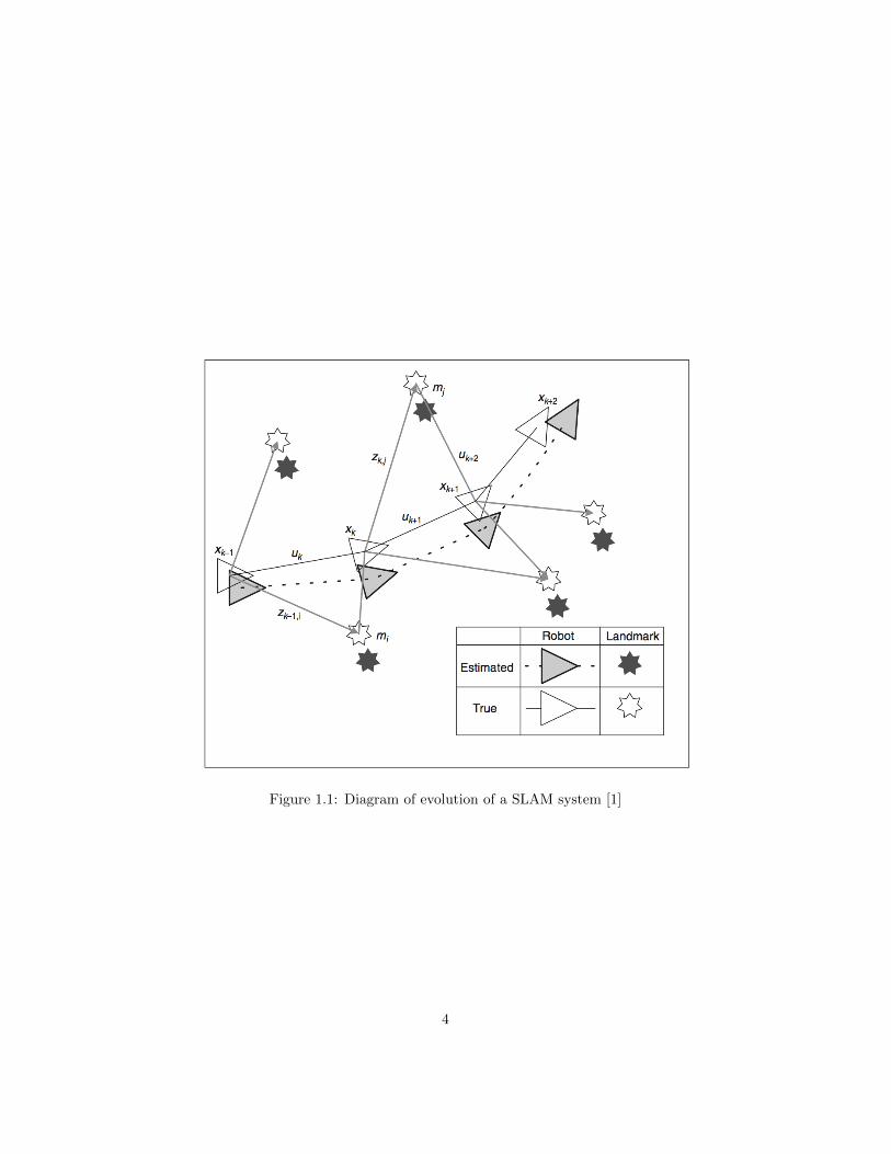
Figure 1.1: Diagram of evolution of a SLAM system [1]

4

Chapter 2

Objective of the Project

The objective of this project was to understand what exactly the SLAM problemwas and to propose a simple solution that could serve as a first approach tosolving the problem.

This solution should be able to obtain an estimate of the position of themoving agent and the features of the map at each time step by using dataobtained from sensors to calculate a more accurate estimate or in other wordsto decrease the uncertainty in the position of the agent and the features. In ourcase the sensors that will be used are a stereo camera system. The data obtainedfrom processing the images has to be all we need to apply the algorithm.

The project also included that this proposed solution could be programmedin C++ using OpenCV library ,with the additional usage of the code and videodata set from Vicomtech’s stereo odometry system [1] which obtained odometrydata from the stereo camera system.

2.1 The System

To be able to apply a SLAM algorithm we first need to define the coordinatesystem in which our features and our agent will be in. There are many waysto define a coordinate system but in the end they must all represent the samemovement and position . In a coordinate system there should always be acoordinate (0,0) or as we may also call it the world starting point. For us thispoint will be the where we obtain the first frames from our camera .

In our coordinate system the localisation or position of the robot will be 6dimensional. The 6 dimensions will be the following :

x y z φ χ ψ

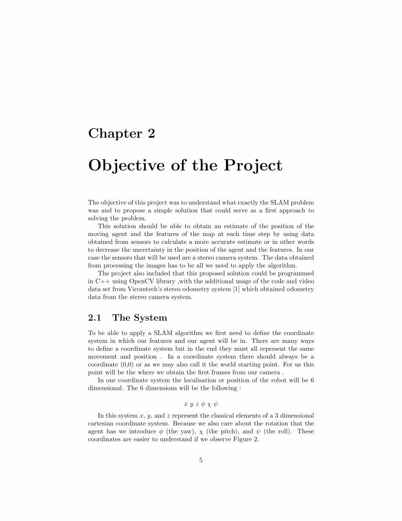
In this system x, y, and z represent the classical elements of a 3 dimensionalcartesian coordinate system. Because we also care about the rotation that theagent has we introduce φ (the yaw), χ (the pitch), and ψ (the roll). Thesecoordinates are easier to understand if we observe Figure 2.

5

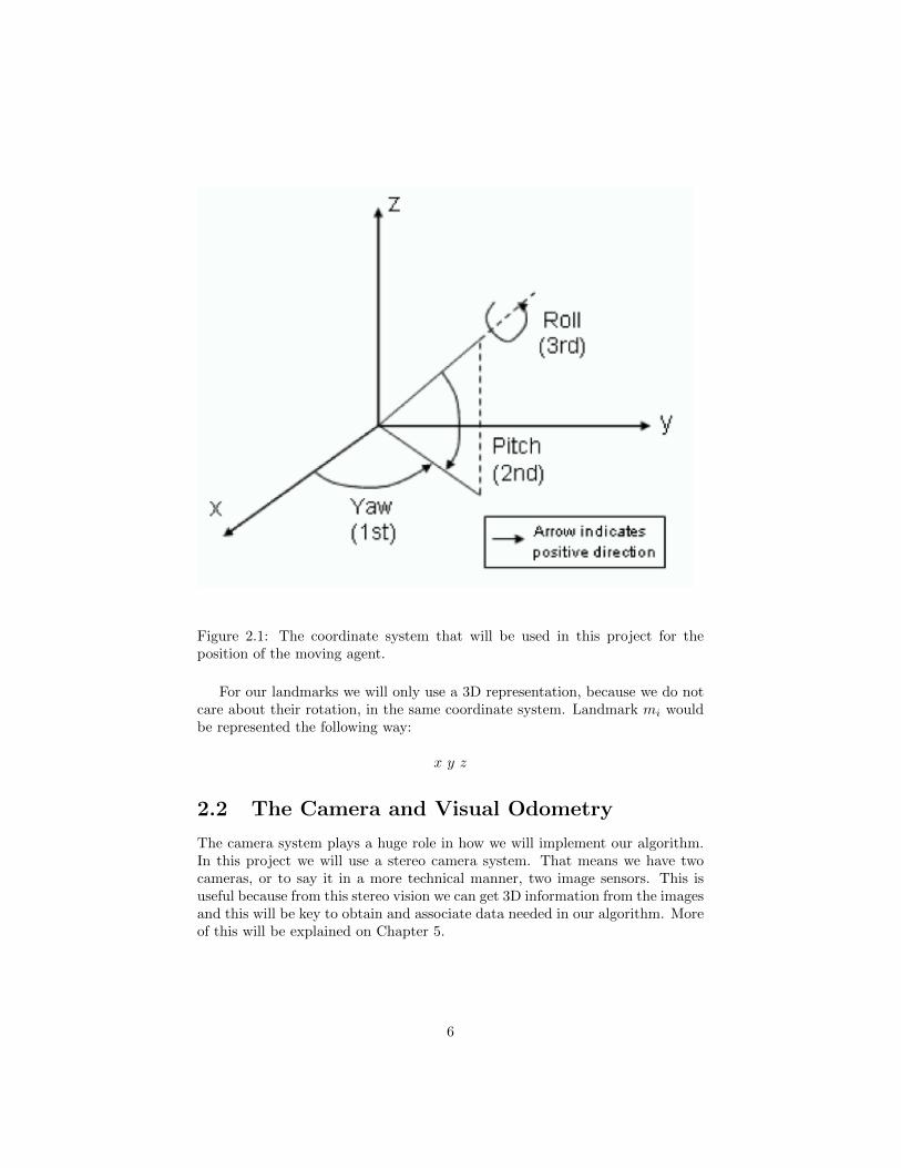
Figure 2.1: The coordinate system that will be used in this project for theposition of the moving agent.

For our landmarks we will only use a 3D representation, because we do notcare about their rotation, in the same coordinate system. Landmark mi wouldbe represented the following way:

x y z

2.2 The Camera and Visual Odometry

The camera system plays a huge role in how we will implement our algorithm.In this project we will use a stereo camera system. That means we have twocameras, or to say it in a more technical manner, two image sensors. This isuseful because from this stereo vision we can get 3D information from the imagesand this will be key to obtain and associate data needed in our algorithm. Moreof this will be explained on Chapter 5.

6

Figure 2.2: An example of a stereo camera system.

As we mentioned previously, code has been inherited from a previous imple-mentation [1]. We will briefly try to explain what it did and how our algorithmwill differ from it.

The code implemented a visual odometry algorithm. Odometry is the use ofdata to obtain change of position over time. In the code the data was obtainedby the cameras. What the code did was from a couple of images taken at thesame time it matched them with OpenCV functions and then triangulated thematched points. At the next time step we would have obtained a couple of newimages. At this new time step we would use a new matching algorithm thatwould make a ”circular” match. That means that the only points consideredgood matches would complete a cycle between the old images and the newimages. With this we obtain 2D matches. Before we had triangulated somepoints from the first couple of images. Because we know which points from 2Dof the original images were the ones triangulated we can observe if any of thesetriangulated points have matches in the new set of 2D images. If they do, thenwhat we have are 3D-2D correspondences. This data will be the input to afunction of OpenCV which obtains a pose or movement of the camera from theoriginal set of images to the new set of images.The algorithm does this everytime step. We have obtained the odometry only from the data from the cameras.

How is this different from our algorithm? The visual odometry will onlycalculate the odometry or pose from a time step to the next one. It does not takeinto account information from previous time steps. That is a key to any SLAMalgorithm. Also, a very important and key difference is that the visual odometry

7

believes that the calculated pose is correct. It does not take into account anypossible source of noise or uncertainty. In SLAM, this is a fundamental step.Every camera system and every computational process will have sources of noiseleading to uncertainty in the results. In our implementation of EKF-SLAM weuse the odometry data not only to estimate the position of the agent but also tocorrect the uncertainty of the agent and of the features position. More of thiswill be explained in Chapter 5.

Because this is only a first approach, the implemented algorithm was in-tended to be simple and not to computationally costly , and that is why ourimplementation does not take into account all of the time steps for the stepsthat will later be explained , but it will be able to keep track of the position ofthe agent through the whole movement in the map, or to say in in other wordsit will keep an absolute position of the robot with respect to the starting point.

2.2.1 Applications of the EKF-SLAM Algorithm

It is easy to see that a successful implementation of the algorithm would dogreat things in the world of navigation. If robots, cars , etc. would be ableto locate themselves in a map (which would also be known) with a small levelof uncertainty these things could become autonomous and they could navigatethemselves.

In present day SLAM is used for both autonomous vehicles but also for as-sistance to the driver. Practical applications can be found everywhere. Fromvacuum cleaners that navigate the house on their own to exploration of under-ground mines by autonomous robots.Perhaps the most popular application inthe present day is the self driving cars. Self driving cars find their basic prin-ciples in SLAM, although they are much more complicated that what we do inthis project because they use several more sensor and they sometimes includeother type of navigation assistance, for example GPS.

One of the most successful and famous implementations of SLAM is theStanley vehicle created by Stanford University’s Stanford Racing Team in coop-eration with the Volkswagen Electronics Research Laboratory (ERL). It com-peted and won the 2005 DARPA challenge, which was a competition fundedby the Defense Advanced Research Projects Agency for autonomous cars in thedesert.

The interest in SLAM is greater each day, and applications, both militaryand civilian, will surely be a big factor in the near future.

8

Chapter 3

Different Approaches toSLAM

In this section we will discuss the most popular and successful approaches ofSLAM over the years.

3.1 The Extended Kalman Filter SLAM

The EKF SLAM(Extended Kalman Filter SLAM) has been the classical ap-proach to solve the SLAM problem. Its basis is in the Kalman filter but it hasa slight difference. To explain it we first need to know what the Kalman filteris.

3.1.1 The Kalman Filter

The Kalman Filter is a technique invented by Rudolph Emil Kalman with thepurpose of filtering and predicting in linear systems. It can only be applied inlinear. This filter represents beliefs at time k by a mean and a covariance ofa state.

The basic idea behind the filter is that we introduce into the filter somenoisy data and our algorithm will give us a less noise or more exact data. Itsapplications can be found in many areas, from economics to computer visionand tracking applications.

We will now show and explain the Kalman filter algorithm.First we aregoing to explain the notation we are going to use briefly. For now the notationof the mean or estimate of our state vector will be x (not to be confused withthe position of the robot xk mentioned previously) and the covariance will beexpressed as P. The notation xn|m will mean that it is the estimate at timen with observations up to, and including time m. It is analog with Pn|m Thealgorithm can be described as follows:

9

xk|k−1 = Fkxk−1|k−1 + Bkuk (3.1)

Pk|k−1 = FkPk−1|k−1FTk + Qk (3.2)

yk = zk −Hkxk|k−1 (3.3)

Sk = HkPk|k−1HTk + Rk (3.4)

Kk = Pk|k−1HTk S−1k (3.5)

xk|k = xk|k−1 + Kkyk (3.6)

Pk|k = (I −KkHk)Pk|k−1 (3.7)

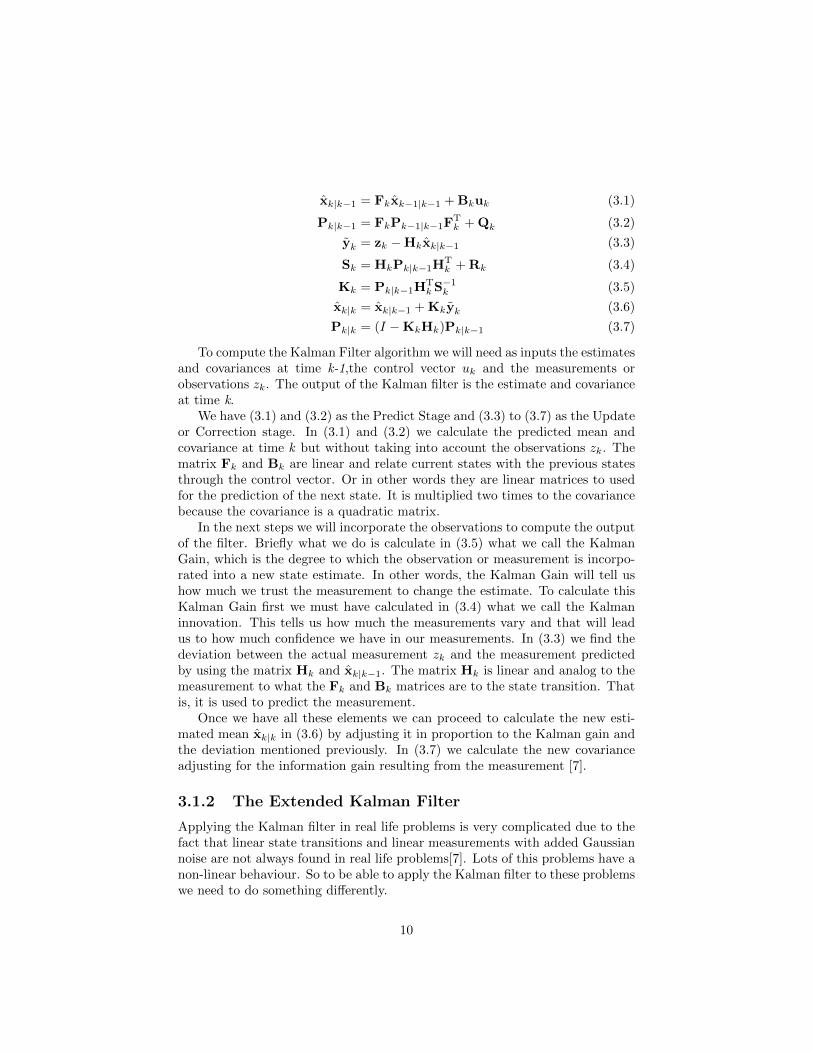
To compute the Kalman Filter algorithm we will need as inputs the estimatesand covariances at time k-1,the control vector uk and the measurements orobservations zk. The output of the Kalman filter is the estimate and covarianceat time k.

We have (3.1) and (3.2) as the Predict Stage and (3.3) to (3.7) as the Updateor Correction stage. In (3.1) and (3.2) we calculate the predicted mean andcovariance at time k but without taking into account the observations zk. Thematrix Fk and Bk are linear and relate current states with the previous statesthrough the control vector. Or in other words they are linear matrices to usedfor the prediction of the next state. It is multiplied two times to the covariancebecause the covariance is a quadratic matrix.

In the next steps we will incorporate the observations to compute the outputof the filter. Briefly what we do is calculate in (3.5) what we call the KalmanGain, which is the degree to which the observation or measurement is incorpo-rated into a new state estimate. In other words, the Kalman Gain will tell ushow much we trust the measurement to change the estimate. To calculate thisKalman Gain first we must have calculated in (3.4) what we call the Kalmaninnovation. This tells us how much the measurements vary and that will leadus to how much confidence we have in our measurements. In (3.3) we find thedeviation between the actual measurement zk and the measurement predictedby using the matrix Hk and xk|k−1. The matrix Hk is linear and analog to themeasurement to what the Fk and Bk matrices are to the state transition. Thatis, it is used to predict the measurement.

Once we have all these elements we can proceed to calculate the new esti-mated mean xk|k in (3.6) by adjusting it in proportion to the Kalman gain andthe deviation mentioned previously. In (3.7) we calculate the new covarianceadjusting for the information gain resulting from the measurement [7].

3.1.2 The Extended Kalman Filter

Applying the Kalman filter in real life problems is very complicated due to thefact that linear state transitions and linear measurements with added Gaussiannoise are not always found in real life problems[7]. Lots of this problems have anon-linear behaviour. So to be able to apply the Kalman filter to these problemswe need to do something differently.

10

The solution to this problem is the extended Kalman filter. What we do hereis that instead of the algorithm being governed by linear matrices we introducenon-linear functions. We will call these functions f and h. The prediction of thenext state and of the measurement will be made by the two nonlinear functions.As a consequence of this we will introduce the Jacobians Fk, which will replaceFk and Bk, and Hk which will replace Hk. Even though we use the same lettersin a couple of matrices we should not confuse them.

The EKF, as it is called, is indeed a solution. But that does not mean thatit does not have its problems. By using the nonlinear function the real belief ofthe state is no longer a Gaussian, but the EKF approximates it as a Gaussian,with a mean and a covariance. That means the belief is no longer exact, as itwas in the Kalman Filter, but it is only an approximation.

In the next subsection we will see the EKF algorithm and the differencesbetween both algorithms will be easier to see and understand.

3.1.3 The EKF Algorithm

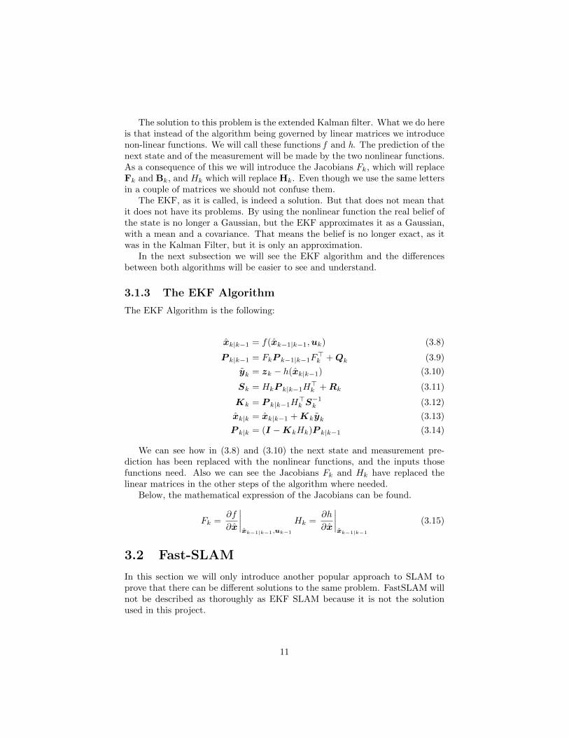
The EKF Algorithm is the following:

xk|k−1 = f(xk−1|k−1,uk) (3.8)

P k|k−1 = FkP k−1|k−1F>k + Qk (3.9)

yk = zk − h(xk|k−1) (3.10)

Sk = HkP k|k−1H>k + Rk (3.11)

Kk = P k|k−1H>k S−1k (3.12)

xk|k = xk|k−1 + Kkyk (3.13)

P k|k = (I −KkHk)P k|k−1 (3.14)

We can see how in (3.8) and (3.10) the next state and measurement pre-diction has been replaced with the nonlinear functions, and the inputs thosefunctions need. Also we can see the Jacobians Fk and Hk have replaced thelinear matrices in the other steps of the algorithm where needed.

Below, the mathematical expression of the Jacobians can be found.

Fk =∂f

∂x

∣∣∣∣xk−1|k−1,uk−1

Hk =∂h

∂x

∣∣∣∣xk−1|k−1

(3.15)

3.2 Fast-SLAM

In this section we will only introduce another popular approach to SLAM toprove that there can be different solutions to the same problem. FastSLAM willnot be described as thoroughly as EKF SLAM because it is not the solutionused in this project.

11

FastSLAM can be practical to use when we have an environment with a bigset of features( in the order of millions). Also when there are many randompatterns, shapes, and textures[8].

In FastSLAM we can say that we handle each feature separately because ofconditional independence according to a Bayesian Network. This will make theprobability distribution to focus on the trajectory of the robot instead of just asingle pose of the robot at a certain time. This is the reason for its speed , as itmakes the map representation a set of independent Gaussians instead of a jointmap covariance like we did in the EFK SLAM. FastSLAM is also called Rao-Blackwellized Filter SLAM because it has the structure of a Rao-Blackwellizedstate. For the pose states recursive estimation is performed with the techniqueof particle filtering and we use EKF for the map states we use the EKF byprocessing each landmark individually as an EKF measurement assuming wehave a known pose[2].

To properly and thoroughly describe FastSLAM we would need to makea whole new project. But what is described previously shows that differenttechniques can be used to solve the problem. This is mentioned in this projectto emphasise the notion that SLAM is more of a concept than just an algorithm,and how it can be solved in different ways and depending on the situation asolution could be better than other.

12

Chapter 4

Methodology

In this Chapter we will briefly explain some of the tools we used to implementour algorithm. Basically the most important tools used in our project wereC++, Matlab and the library for C++ OpenCV.

We will not explain the C++ tools used the code used for C++ was verybasic mostly because if we wanted to use a special function, class or feature weused them from the OpenCV library.

4.1 OpenCV Library

This library is a great tool to use if images are involved. Also, because imagescan be represented as matrices the library is very useful when handling matrices.

The most important functions and classes used in the code were:GridAdaptedFeatureDetector: According to the OpenCv website this class

adapts a detector to partition the source image into a grid and detect points ineach cell. With an object of this class and the detect function of this class wecan detect points in an image.

BriefDescriptorExtractor: An object of this class will compute BRIEF de-scriptors. Descriptors are like the characteristics of each point detected in theimage.With the compute function of this class the descriptors of each point willbe created.

class DescriptorMatcher: Class for matching descriptors. With the matchfunction we can match the descriptors to see with point has a correspondencein other image.

triangulatePoints: This function reconstructs 3D points by triangulation ofcorrespondences.

Point3d: This class allows us to create variables of this class and for themto be 3 dimensional. Another example would be Point3f, which would create a3D point of floats.

class Mat: This is probably our most used class. All of our matrices areobjects of the Mat class. This class allows us to directly do operations on

13

matrices and one of the most interesting and used functions is the rect() functionwhich lets us copy or insert just a ”rectangle” or a portion of the matrix. Theimportance of this function will be seen later on this project when the operationsfor the implementation appear.

These are the most important and most used functions and classes we haveused in our implementation and that make the handling of images possible andeasier in C++.

4.2 Matlab

Later on this project we will find that we need to compute some Jacobians. TheJacobians are basically derivatives and with the type of matrices that we havecomputing this by hand would be impossible. And a feasible implementationof derivatives in C++ or OpenCV was not an option. That is why we usedthe Matlab symbolic toolbox. In this toolbox we can define some variablesand all of the results from the operations done regarding that variable will bein function of the variable. This was helpful because we could just insert thegeneral expression in matlab and the result would always be in function of thevariables we wanted. The usage of this will be easily seen when the operations forthe Jacobians are reached and also the Matlab code can be found in AppendixA.

14

Chapter 5

Implementation of the EKFSLAM

5.1 System Specific Matrices of EKF SLAM

In this section and the ones that follow we will describe the implementationof the EKF SLAM applied to our specific system .We will have a very similarsystem and theoretical implementation as the one used by Jose-Luis Blanco inhis report “Derivation and Implementation of a Full 6D EKF-based Solution toBearing-Range SLAM” [9].

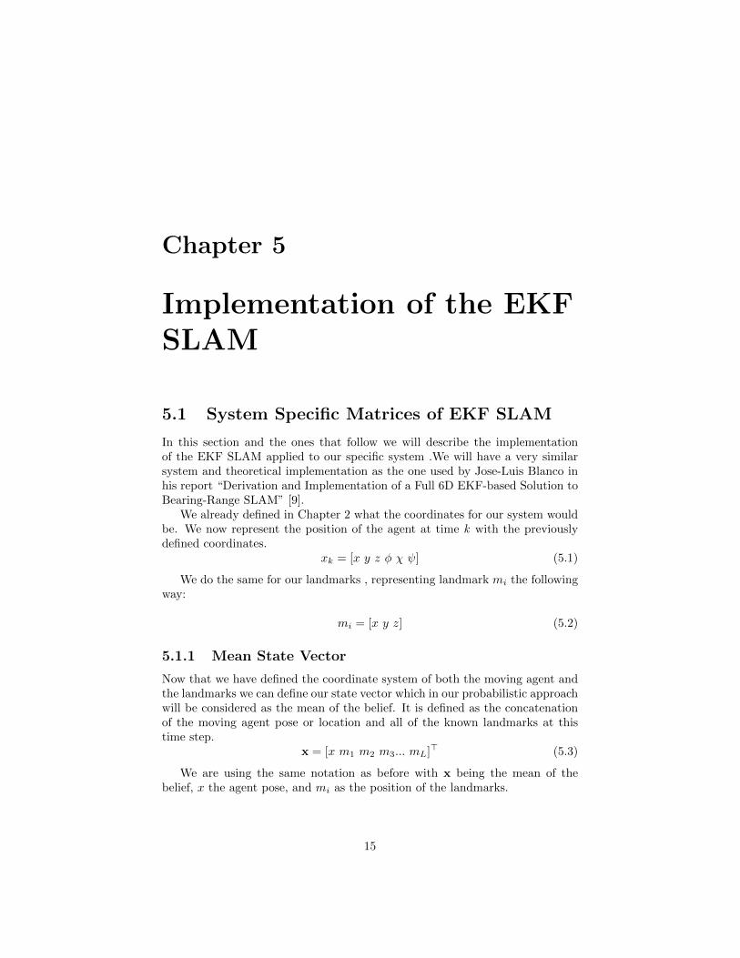
We already defined in Chapter 2 what the coordinates for our system wouldbe. We now represent the position of the agent at time k with the previouslydefined coordinates.

xk = [x y z φ χ ψ] (5.1)

We do the same for our landmarks , representing landmark mi the followingway:

mi = [x y z] (5.2)

5.1.1 Mean State Vector

Now that we have defined the coordinate system of both the moving agent andthe landmarks we can define our state vector which in our probabilistic approachwill be considered as the mean of the belief. It is defined as the concatenationof the moving agent pose or location and all of the known landmarks at thistime step.

x = [x m1 m2 m3... mL]> (5.3)

We are using the same notation as before with x being the mean of thebelief, x the agent pose, and mi as the position of the landmarks.

15

When implementing the EKF SLAM in C++ we will initialise the robotpose to all zeros, as we belief this is the starting point.

As for the landmarks, we will briefly explain how we obtain them using thecode provided by Vicomtech [1] and some code added by myself to adjust it intothe EKF algorithm.

When we have our first camera pair, that is at time k = 0 we detect featuresin our image using both cameras and using a procedure(which explanation isout of the boundaries of this project) we try to keep only the features that webelieve have a correspondence in the other image, in other words we match thefeatures in one image to the other image as best as we can. There will alwaysbe some outliers and these will contribute to the noise in our system. Thosepoints will be considered our first set of landmarks. To properly introduce theminto our mean state vector we need to know their absolute coordinates referredto the world starting point.

As mentioned previously, we have decided that we are currently at the worldstarting point. Because of this and because of our stereo camera system we onlyneed to triangulate the matching points in our images and once we convert thedistance obtained from the triangulation to world coordinates instead of pixelcoordinates we already have the distance from the world starting point to all ofthe landmarks. They are ready to be introduced to our mean state vector.

We use the functions provided by OpenCV and explained in Chapter 4 tomatch and triangulate these points.

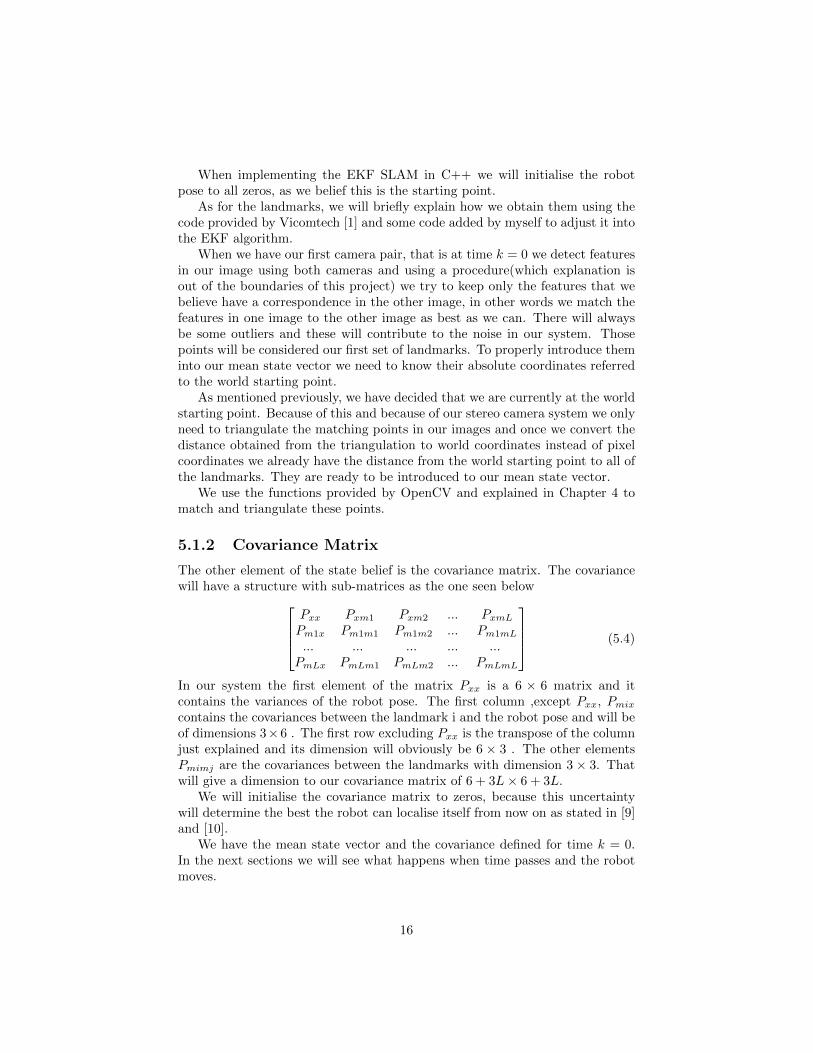
5.1.2 Covariance Matrix

The other element of the state belief is the covariance matrix. The covariancewill have a structure with sub-matrices as the one seen below

Pxx Pxm1 Pxm2 ... PxmL

Pm1x Pm1m1 Pm1m2 ... Pm1mL

... ... ... ... ...PmLx PmLm1 PmLm2 ... PmLmL

(5.4)

In our system the first element of the matrix Pxx is a 6 × 6 matrix and itcontains the variances of the robot pose. The first column ,except Pxx, Pmix

contains the covariances between the landmark i and the robot pose and will beof dimensions 3×6 . The first row excluding Pxx is the transpose of the columnjust explained and its dimension will obviously be 6 × 3 . The other elementsPmimj are the covariances between the landmarks with dimension 3× 3. Thatwill give a dimension to our covariance matrix of 6 + 3L× 6 + 3L.

We will initialise the covariance matrix to zeros, because this uncertaintywill determine the best the robot can localise itself from now on as stated in [9]and [10].

We have the mean state vector and the covariance defined for time k = 0.In the next sections we will see what happens when time passes and the robotmoves.

16

5.2 First Step: Prediction

In this section we will discuss the specific elements and the implementation offirst two steps of the EKF algorithm which are stated in (3.8) and (3.9).

5.2.1 The Motion Model

The only variables that are affected by time and therefore movement are thosebelonging to the pose of the agent. The landmarks we consider static with time.

Lets remember the first step of the EKF filter :

xk|k−1 = f(xk−1|k−1,uk)

with f being a nonlinear function. This function is they key to predict xk|k−1.Inour system . It’s important to realise that we need the inputs xk−1|k−1 and uk

being the previous mean state vector and the control vector. With this inputswe will construct the motion model to make the prediction of the mean.

The control vector uk can be expressed as

u = {xu yu zu φu χu ψu} (5.5)

We know from (5.1) how our state vector mean is expressed but becauseof rotations in movements we can’t just add x + xu and so on to obtain themotion model. What we need to do is use the pose composition operator ⊕to obtain the new pose. The composition operator is equivalent to multiplyingtheir equivalent homogeneous matrices.

f(xk−1|k−1,uk) = xk−1|k−1 ⊕ uk (5.6)

To do this we need to be able to express the control and the pose in homoge-neous matrix form. Both of this matrices can be obtained in homogeneous formfrom their elements xu , yu , zu , φu , χu and ψu using the following formula

R11 R12 R13 xR21 R22 R23 yR31 R32 R33 z0 0 0 1

=

cosφcosχ cosφsinχsinψ − sinφcosψ cosφsinχcosψ + sinφsinψ xsinφcosχ sinφsinχsinψ + cosφcosψ sinφsinχcosψ − cosφsinψ y−sinχ cosχsinψ cosχcosψ z

0 0 0 1

(5.7)

17

We can consider the homogeneous matrix can be divided into c 3×3 rotationsub matrix and a 3× 1 translation sub matrix not taking into account the lastrow.

The result of the composition operator would be another homogeneous ma-trix. We are interested in obtaining the the elements x , y , z , φ , χ and ψ of theresulting homogenous matrix. If we write individually for each element whatthe composition operator yielded we obtain the following.

xk = xk−1 +R11xu +R12yu +R13zu (5.8)

yk = yk−1 +R21xu +R22yu +R23zu (5.9)

zk = zk−1 +R31xu +R32yu +R33zu (5.10)

φk = φk−1 + φu (5.11)

χk = χk−1 + χu (5.12)

ψk = ψk−1 + ψu (5.13)

(5.14)

Note that for the yaw, pitch and roll we have not really put the operationsmade by the composition operator, but we just add the previous angle with theangle added by the control. We do this because in the case of the angles it ispossible to add them and we can obtain them directly from the rotation matrixof the resulting homogeneous matrix (from the composition operator).

In the implementation in C++ instead of obtaining the correspondent yaw,pitch, and roll two times, one for the control matrix and one for the previouspose matrix, we can directly obtain the values of the yaw, pitch, and roll fromthe resulting matrix of the composition operator to be more efficient. We cando it using the following algorithm from [11].

yaw = atan2(R32, R33) (5.15)

c2 =√R2

32 +R233 (5.16)

pitch = atan2(−R31, c2) (5.17)

roll = atan2(R21, R11) (5.18)

What we have in (5.8) to (5.14) is also our motion model which shows ushow the our mean pose will change with time. This seems to work fine, but toapply it we need to obtain the inputs correctly.

5.2.2 Obtaining control from visual odometry

As we saw in the previous section once we have the inputs it is possible to builda motion model. In this subsection it will be briefly and shallowly explainedhow we obtain the controls from Vicomtech’s stereo odometry system [1]. Mostof this has already been explained in subsection 2.2.1 but here we will try toexplain it again and explaining in a deeper way the ”circular” match.

18

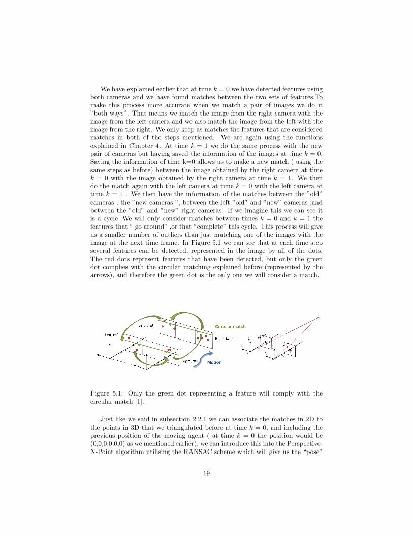
We have explained earlier that at time k = 0 we have detected features usingboth cameras and we have found matches between the two sets of features.Tomake this process more accurate when we match a pair of images we do it”both ways”. That means we match the image from the right camera with theimage from the left camera and we also match the image from the left with theimage from the right. We only keep as matches the features that are consideredmatches in both of the steps mentioned. We are again using the functionsexplained in Chapter 4. At time k = 1 we do the same process with the newpair of cameras but having saved the information of the images at time k = 0.Saving the information of time k=0 allows us to make a new match ( using thesame steps as before) between the image obtained by the right camera at timek = 0 with the image obtained by the right camera at time k = 1. We thendo the match again with the left camera at time k = 0 with the left camera attime k = 1 . We then have the information of the matches between the ”old”cameras , the ”new cameras ”, between the left ”old” and ”new” cameras ,andbetween the ”old” and ”new” right cameras. If we imagine this we can see itis a cycle .We will only consider matches between times k = 0 and k = 1 thefeatures that ” go around” ,or that ”complete” this cycle. This process will giveus a smaller number of outliers than just matching one of the images with theimage at the next time frame. In Figure 5.1 we can see that at each time stepseveral features can be detected, represented in the image by all of the dots.The red dots represent features that have been detected, but only the greendot complies with the circular matching explained before (represented by thearrows), and therefore the green dot is the only one we will consider a match.

Figure 5.1: Only the green dot representing a feature will comply with thecircular match [1].

Just like we said in subsection 2.2.1 we can associate the matches in 2D tothe points in 3D that we triangulated before at time k = 0, and including theprevious position of the moving agent ( at time k = 0 the position would be(0,0,0,0,0,0) as we mentioned earlier), we can introduce this into the Perspective-N-Point algorithm utilising the RANSAC scheme which will give us the “pose”

19

of the agent from 3D-2D point correspondences. We can implement it directlyusing the the PnPRansac function from OpenCV library for C++. In realitythe “pose” that the function gives us is the “pose” from k = 0 to k = 1, whichis what we call the control.

Next we triangulate the matches from the new left and right images. In thenext time frame these new images and all of its information will become the oldimages and repeats itself iteratively. This is how we obtain the control at everytime step from k to k + 1.

5.2.3 Predicted State Vector xk|k−1

We can directly apply equations (5.8) to (5.14) using the control obtained fromthe odometry process explained before and the previous location of the movingagent to obtain

xk|k−1

, which is the predicted mean state vector without having taken into account theobservations. It may seem we have taken into account the observations becausethe process to obtain the control uses the matches. But this process uses thematches as an input to the RANSAC algorithm which selects only a number ofall the matches, and this process has its own source of noise when estimatingthe pose.

As we said before only the position of the agent is affected by time, aslandmarks are considered static. That is why we only observe the position ofthe robot being affected in the motion model.

5.2.4 Predicted Covariance Matrix Pk|k−1

To complete the prediction stage the next step is to predict the covariance matrixnot taking into account the observations yet. For this we need the covariancematrix at the previous time step P k−1|k−1,the Jacobian Fk , and a matrix whichis the uncertainty associated to the movement of the agent, Qk .

Jacobian Fk

The mathematical expression to obtain the Jacobian Fk was the following :

Fk =∂f

∂x

∣∣∣∣xk|k−1,uk−1

.

We know the operations function f makes ,so if we apply the definition ofJacobian, that is the matrix of all first-order partial derivatives of a vector-valued function we obtain the following:

Fk =

∂f∂x

∣∣∣6x6

0|6x3 0|6x3 ... 0|6x30|3x6 I|3x3 0|3x3 ... 0|3x3... ... ... ... ...

0|3x6 0|3x3 0|3x3 ... I|3x3

(5.19)

20

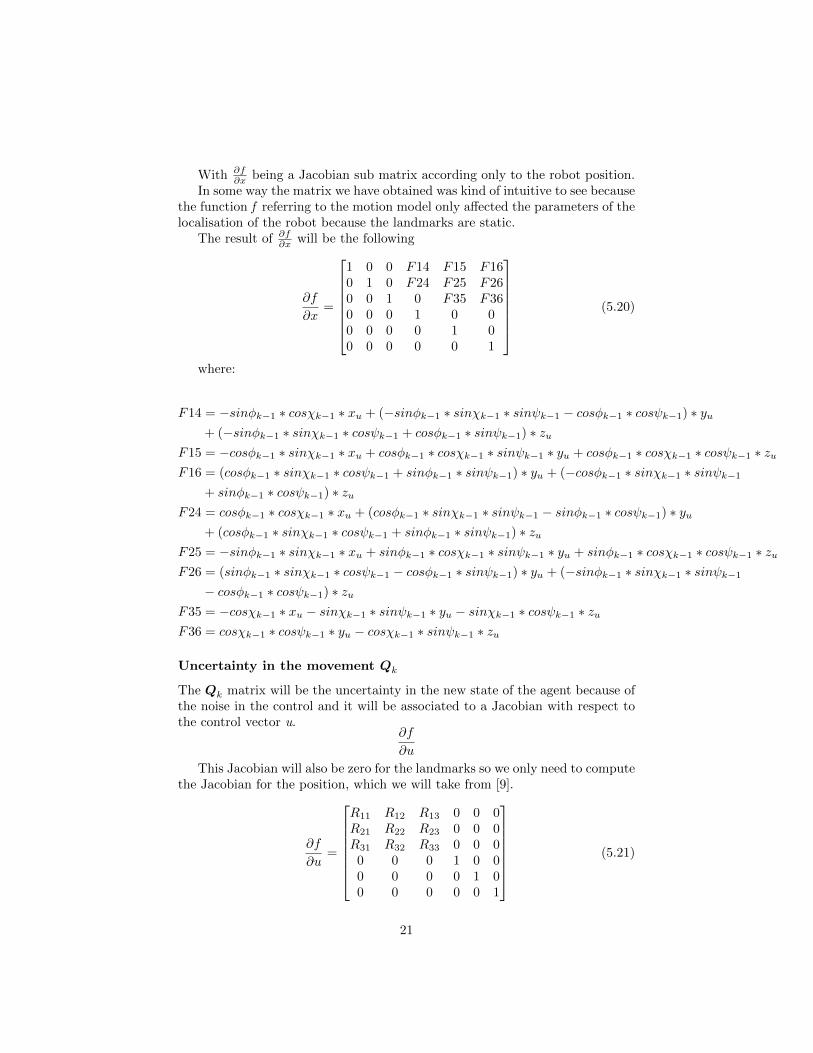
With ∂f∂x being a Jacobian sub matrix according only to the robot position.

In some way the matrix we have obtained was kind of intuitive to see becausethe function f referring to the motion model only affected the parameters of thelocalisation of the robot because the landmarks are static.

The result of ∂f∂x will be the following

∂f

∂x=

1 0 0 F14 F15 F160 1 0 F24 F25 F260 0 1 0 F35 F360 0 0 1 0 00 0 0 0 1 00 0 0 0 0 1

(5.20)

where:

F14 = −sinφk−1 ∗ cosχk−1 ∗ xu + (−sinφk−1 ∗ sinχk−1 ∗ sinψk−1 − cosφk−1 ∗ cosψk−1) ∗ yu+ (−sinφk−1 ∗ sinχk−1 ∗ cosψk−1 + cosφk−1 ∗ sinψk−1) ∗ zu

F15 = −cosφk−1 ∗ sinχk−1 ∗ xu + cosφk−1 ∗ cosχk−1 ∗ sinψk−1 ∗ yu + cosφk−1 ∗ cosχk−1 ∗ cosψk−1 ∗ zuF16 = (cosφk−1 ∗ sinχk−1 ∗ cosψk−1 + sinφk−1 ∗ sinψk−1) ∗ yu + (−cosφk−1 ∗ sinχk−1 ∗ sinψk−1

+ sinφk−1 ∗ cosψk−1) ∗ zuF24 = cosφk−1 ∗ cosχk−1 ∗ xu + (cosφk−1 ∗ sinχk−1 ∗ sinψk−1 − sinφk−1 ∗ cosψk−1) ∗ yu

+ (cosφk−1 ∗ sinχk−1 ∗ cosψk−1 + sinφk−1 ∗ sinψk−1) ∗ zuF25 = −sinφk−1 ∗ sinχk−1 ∗ xu + sinφk−1 ∗ cosχk−1 ∗ sinψk−1 ∗ yu + sinφk−1 ∗ cosχk−1 ∗ cosψk−1 ∗ zuF26 = (sinφk−1 ∗ sinχk−1 ∗ cosψk−1 − cosφk−1 ∗ sinψk−1) ∗ yu + (−sinφk−1 ∗ sinχk−1 ∗ sinψk−1

− cosφk−1 ∗ cosψk−1) ∗ zuF35 = −cosχk−1 ∗ xu − sinχk−1 ∗ sinψk−1 ∗ yu − sinχk−1 ∗ cosψk−1 ∗ zuF36 = cosχk−1 ∗ cosψk−1 ∗ yu − cosχk−1 ∗ sinψk−1 ∗ zu

Uncertainty in the movement Qk

The Qk matrix will be the uncertainty in the new state of the agent because ofthe noise in the control and it will be associated to a Jacobian with respect tothe control vector u.

∂f

∂u

This Jacobian will also be zero for the landmarks so we only need to computethe Jacobian for the position, which we will take from [9].

∂f

∂u=

R11 R12 R13 0 0 0R21 R22 R23 0 0 0R31 R32 R33 0 0 00 0 0 1 0 00 0 0 0 1 00 0 0 0 0 1

(5.21)

21

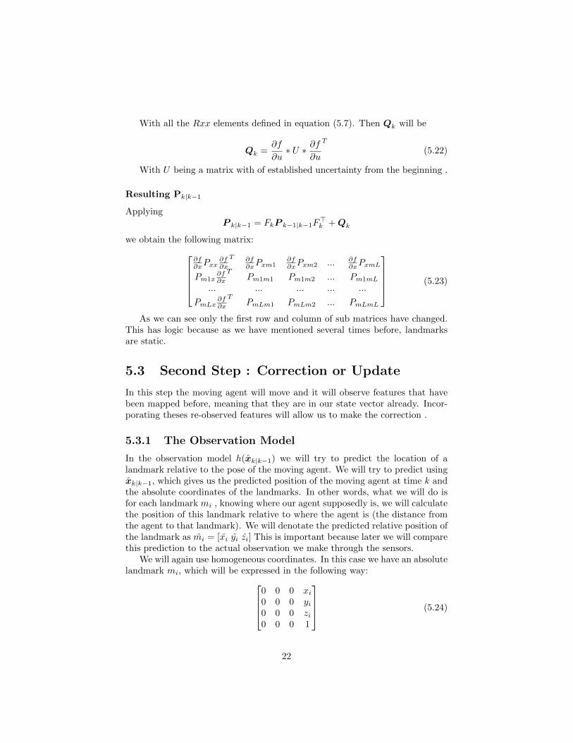
With all the Rxx elements defined in equation (5.7). Then Qk will be

Qk =∂f

∂u∗ U ∗ ∂f

∂u

T

(5.22)

With U being a matrix with of established uncertainty from the beginning .

Resulting Pk|k−1

ApplyingP k|k−1 = FkP k−1|k−1F

>k + Qk

we obtain the following matrix:∂f∂xPxx

∂f∂x

T ∂f∂xPxm1

∂f∂xPxm2 ... ∂f

∂xPxmL

Pm1x∂f∂x

TPm1m1 Pm1m2 ... Pm1mL

... ... ... ... ...

PmLx∂f∂x

TPmLm1 PmLm2 ... PmLmL

(5.23)

As we can see only the first row and column of sub matrices have changed.This has logic because as we have mentioned several times before, landmarksare static.

5.3 Second Step : Correction or Update

In this step the moving agent will move and it will observe features that havebeen mapped before, meaning that they are in our state vector already. Incor-porating theses re-observed features will allow us to make the correction .

5.3.1 The Observation Model

In the observation model h(xk|k−1) we will try to predict the location of alandmark relative to the pose of the moving agent. We will try to predict usingxk|k−1, which gives us the predicted position of the moving agent at time k andthe absolute coordinates of the landmarks. In other words, what we will do isfor each landmark mi , knowing where our agent supposedly is, we will calculatethe position of this landmark relative to where the agent is (the distance fromthe agent to that landmark). We will denotate the predicted relative position ofthe landmark as mi = [xi yi zi] This is important because later we will comparethis prediction to the actual observation we make through the sensors.

We will again use homogeneous coordinates. In this case we have an absolutelandmark mi, which will be expressed in the following way:

0 0 0 xi0 0 0 yi0 0 0 zi0 0 0 1

(5.24)

22

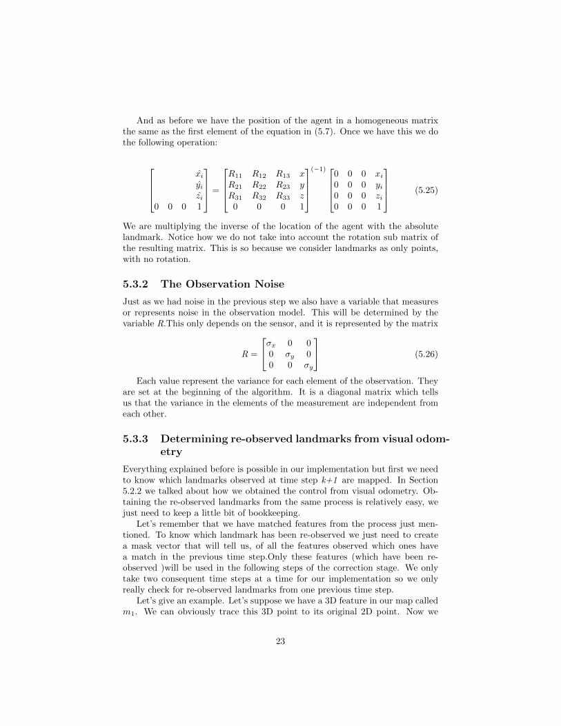
And as before we have the position of the agent in a homogeneous matrixthe same as the first element of the equation in (5.7). Once we have this we dothe following operation:

xiyizi

0 0 0 1

=

R11 R12 R13 xR21 R22 R23 yR31 R32 R33 z0 0 0 1

(−1)

0 0 0 xi0 0 0 yi0 0 0 zi0 0 0 1

(5.25)

We are multiplying the inverse of the location of the agent with the absolutelandmark. Notice how we do not take into account the rotation sub matrix ofthe resulting matrix. This is so because we consider landmarks as only points,with no rotation.

5.3.2 The Observation Noise

Just as we had noise in the previous step we also have a variable that measuresor represents noise in the observation model. This will be determined by thevariable R.This only depends on the sensor, and it is represented by the matrix

R =

σx 0 00 σy 00 0 σy

(5.26)

Each value represent the variance for each element of the observation. Theyare set at the beginning of the algorithm. It is a diagonal matrix which tellsus that the variance in the elements of the measurement are independent fromeach other.

5.3.3 Determining re-observed landmarks from visual odom-etry

Everything explained before is possible in our implementation but first we needto know which landmarks observed at time step k+1 are mapped. In Section5.2.2 we talked about how we obtained the control from visual odometry. Ob-taining the re-observed landmarks from the same process is relatively easy, wejust need to keep a little bit of bookkeeping.

Let’s remember that we have matched features from the process just men-tioned. To know which landmark has been re-observed we just need to createa mask vector that will tell us, of all the features observed which ones havea match in the previous time step.Only these features (which have been re-observed )will be used in the following steps of the correction stage. We onlytake two consequent time steps at a time for our implementation so we onlyreally check for re-observed landmarks from one previous time step.

Let’s give an example. Let’s suppose we have a 3D feature in our map calledm1. We can obviously trace this 3D point to its original 2D point. Now we

23

have the 2D point that originated the 3D point which is in our map. Let’s callthis 2D point m12D . As we said previously when we have a new time step wematch the old images (the images that contain m12D ) with the new images. Soafter we have matched we have several correspondences between the old imagesand the new images. If m12D is among these matches then it means that the3D point m1 has been observed again and we will use it for the correction step.The mas vector that we talk about is just a logical vector(1 or 0) that tells usif a point like m12D has a match in the new time step. We do this with all the3D points from the old time step.

This is extremely important because these re-observed features will allow usto apply the correction step in the Extended Kalman Filter.

5.3.4 Kalman Innovation and Gain

In (3.5) we have the formula to obtain the Kalman gain. To obtain it we needJacobian Hk, our predicted covariance matrix, and innovation Sk .

Full Matrix S

If we directly apply (3.11) we would obtain a full matrix of size 6 + 3L×6 + 3L.According to [9] a way to speed up the implementation is to take advantage ofthe special structure of Hk ( which will be explained later ) and to calculateSi,j as a scalar of the jth component of the ith observed landmark.

Scalar Si,j

To do this we need to take the elements of the observation one at a time.According to [9] the resulting scalar will be the following

∂hi,j∂x

Pxx∂hi,j∂x

T

+ 2∂hi,j∂mi

Pmix∂hi,j∂xi

T

+∂hi,j∂mi

Pmimi∂hi,j∂mi

T

+Rjj (5.27)

where the partial Jacobians are the j’th row of∂hi,j

∂x and Rjj is the j’thdiagonal element of R.

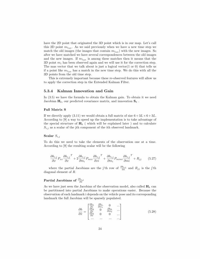
Partial Jacobians of∂hi,j

∂x

As we have just seen the Jacobian of the observation model, also called Hk canbe partitioned into partial Jacobians to make operations easier. Because theobservation of each landmark i depends on the vehicle pose and its correspondinglandmark the full Jacobian will be sparsely populated.

∂h

∂x=

∂h1

∂x∂h1

∂m10 ...

∂h2

∂x 0 ∂h2

∂m2...

∂h3

∂x 0 0 ...... ... ... ...

(5.28)

24

This mean that in reality we only need to computer the partial Jacobians∂hi

∂x and ∂hi

∂mifor each landmark. And each row:

∂hi,j∂x

=[∂hi,j

∂x ...∂hi,j

∂yi...]

(5.29)

with j = 1, 2, 3 corresponds to each of the 3 components of the observation.To obtain the partial Jacobians we have used the symbolic toolbox by mat-

lab. This equations are too big and complicated to put into the project so thecode to obtain them is in appendix A.

Kalman Gain Vector Ki,j

Just as we converted S into Si,j we can also convert the Kalman gain to Ki,j

for a more efficient algorithm. Just as [9] we obtain the following:

Ki,j =

Pxx

Py1x

Py2x

...

∂hi,j

∂x

T+

Pxyi

Py1yi

Py2yi

...

∂hi,j

∂yi

T

1/Si,j (5.30)

5.3.5 Correcting State Vector and Covariance Matrix

We could directly apply (3.13) to correct the state vector. It is very important tonotice the importance of (3.10) which we have not explicitly explained before. Itis the subtraction between the actual value of the observation made through thesensors and the predicted value of the observation made through the observationmodel.

But because we have made some changes to be more efficient, the operationwe will make is

xk|k = xk|k−1 + Ki,j(zi,j − mi,j) (5.31)

With (zi,j − mi,j) being the difference between the actual observation andthe predicted observation.

As for the covariance matrix we will apply the following formula:

P k|k = P k|k−1 − Si,jKi,jKTi,j (5.32)

We will do this for each dimension of each observed landmark.

5.4 Third Step : Creating New Landmarks

We previously mentioned that we would only take two consequent time steps foreach operation. That means that our implemented algorithm behaves as if onlythe images and information at time step k and time step k+1 existed. At timestep k+2 everything is reset except for the agent localisation, so k+1, and itsrelated information, is treated as if it were the beginning of the whole process.This was made to make it a more doable project. Because of this we really do

25

not add any more landmarks at each new time step, because the landmarks ofthe map will only be the ones at the previous time step and at the next time stepthe landmarks of the map will be only the landmarks detected and triangulatedat that time step.

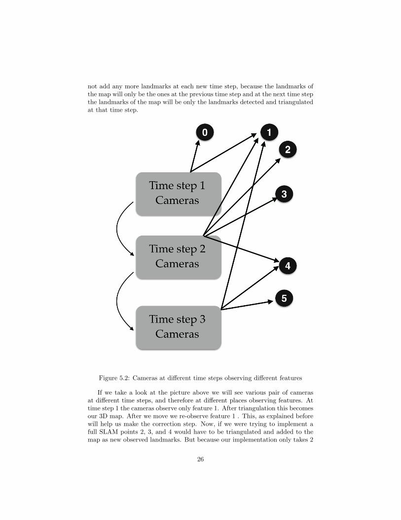
Figure 5.2: Cameras at different time steps observing different features

If we take a look at the picture above we will see various pair of camerasat different time steps, and therefore at different places observing features. Attime step 1 the cameras observe only feature 1. After triangulation this becomesour 3D map. After we move we re-observe feature 1 . This, as explained beforewill help us make the correction step. Now, if we were trying to implement afull SLAM points 2, 3, and 4 would have to be triangulated and added to themap as new observed landmarks. But because our implementation only takes 2

26

time steps at a time we will triangulate the points seen at time step 2 ( 1,2,3,4)and now this will be our new 3D map. Notice that point 0 has been seen onlyby the cameras at time step 1, so this point 0 would not be in our new 3Dmap because we have forgotten about the 3D map created at time step 1. Nowafter we move to time step 3 we re-observe point 4. Again this will help uswith the correction step. Now imagine that at this time step we would havealso observed point 0. This point would have not helped in our implementationbecause we have forgotten about the 3D map from time step 1. A full SLAMimplementation would have not forgotten about it and used it as another pointfor the correction step. After this we would only triangulate points 4, 5, and 1to be our new 3D map.

Having said this, this step is very important to functional SLAM algorithmand that is why we will briefly explain it very theoretically.

After step 2, when we observe landmarks at a new time step k+1 that arealready mapped , and we make all the correct stage operations thank to thesere-observed landmarks, we would like to introduce the landmarks observed atk+1 that were not previously mapped. This will make our map richeras we move through the environment. To do this we will utilise the inverseobservation model. In this model we have a observed landmark relative to theagent and we want to make this landmark absolute to the world coordinates.Again utilising homogeneous coordinates what we do is apply the compositionoperator between the localisation of the moving agent and the observation z atthat time step to obtain the absolute coordinates.

mnew = xk+1 ⊕ zk+1 (5.33)

In the last column we would obtain the coordinates x, y, z that would bethe absolute coordinates of that new landmark.

We would also have add information to the covariance matrix. We wouldhave to add a new row and column to the covariance matrix.

Pxx Pxm1 Pxm2 ... Pxx

∂mnew

∂x

T

Pm1x Pm1m1 Pm1m2 ... Pm1x∂mnew

∂x

T

... ... ... ... ...∂mnew

∂x Pxx∂mnew

∂x Pxm1∂mnew

∂x PmLm2 ... A

(5.34)

With L representing the landmark we have just introduced to the map, and∂mnew

∂x representing the Jacobian of the inverse observation function respect thelocalisation of the moving agent. A represents the following equation:

∂mnew

∂xPxx

∂mnew

∂x

T

+∂mnew

∂zLR∂mnew

∂zL

T

(5.35)

With zL being the observation of the landmark.It is rarely found a full SLAM solution that keeps track of all previous time

steps. Most solutions use windows which focus only on a finite and sometimes

27

small number of time steps that allows the algorithm to be functional, efficientand at the same time robust enough.

28

Chapter 6

Results

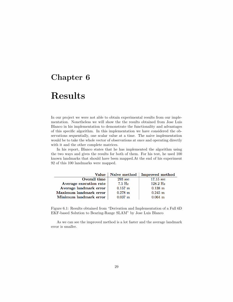
In our project we were not able to obtain experimental results from our imple-mentation. Nonetheless we will show the the results obtained from Jose LuisBlanco in his implementation to demonstrate the functionality and advantagesof this specific algorithm. In this implementation we have considered the ob-servations sequentially, one scalar value at a time. The naive implementationwould be to take the whole vector of observations at once and operating directlywith it and the other complete matrices.

In his report, Blanco states that he has implemented the algorithm usingthe two ways and gives the results for both of them. For his test, he used 100known landmarks that should have been mapped.At the end of his experiment92 of this 100 landmarks were mapped.

Figure 6.1: Results obtained from “Derivation and Implementation of a Full 6DEKF-based Solution to Bearing-Range SLAM” by Jose Luis Blanco

As we can see the improved method is a lot faster and the average landmarkerror is smaller.

29

Chapter 7

Budget

In this Chapter a budget for this project or for any that tries to study a similarsolution will be given.

7.1 Working Hours

The budget for the working hour of this project is given in Table 7.1

Details Hours Cost/Hour Cost

Engineer Hours 260 12 e 3120 eVicomtech PhD/Supervisor Hours 70 35 e 2450 eTECNUN PhD/Supervisor Hours 30 35 e 1050 e

Table 7.1: Working hours budget

7.2 Hardware and Software

Details Usage Hours Cost/Hour Cost

Desktop Computer 260 4,61 e 1200 eVisual Studio C++ 190 0 e 0 e

Matlab Student Suite 10 6,9 e 69 eOpenCV Library 190 0 e 0 e

Table 7.2: Hardware and Software budget

30

Chapter 8

Conclusions

In the implementation , even though the code was compiled, logical experimentalresults could not be obtained.

However, we have given a theoretical solution to this slam problem in oursystem and created a code implementing many of the steps that could lead toa full slam solution.

This project has, first of all, reused the code from [1] to transform the odom-etry data into data that can serve as input for an EKF-SLAM algorithm. Thisproject also has properly implemented all the mathematical operations betweenmatrices needed to compute the EKF algorithm. Most of this operations havebeen done by taking advantage of the OpenCV library and the functions it of-fers for treating matrices, for example the rect() function, and as the resultsfrom Jose Luis Blanco say, this implementations is faster and more robust thana naive implementation. A solution to finding Jacobians was also found andimplements using the Matlab symbolic toolbox. This is very helpful for futurework in this subject.

Also data has been successfully associated, creating mask vectors that allowus to differentiate between re-observed landmarks and landmarks not observedyet.The framework for a future full slam solution that takes into account all thetime steps 3D features has also been established for future work.

Finally all this was put together to create a compilable code that shouldimplement a first approach solution to a SLAM problem. As it happens manytimes there are bugs and small errors that have not permitted coherent resultsto be taken from this project.

In the next Chapter we will try to give a couple of improvements that couldmake our project functional or more efficient.

31

Chapter 9

Future Work

Obvious work has to be done on correcting the probable errors mentioned beforebut in this Chapter the following steps that I think should be followed to makethis solution a feasible one will be presented.

9.1 Improvements in algorithm

As we have seen we only take two consequent time steps for the operations. Afull SLAM solution would need to at least take into account a small window tohave a more robust map. Because of how we do the matching this really becomesa problem of code because the complication is the need to arrange, save andkeep track every observed feature to realise if it has ever been seen before ornot. Another option for this is, instead of keeping the masks, just keeping allthe previous points and make a new matching algorithm. The question is ifthis would be computationally effective. The most probable errors can be foundin the covariance matrix which we have defined with arbitrary values, used bysome other implementations that have been posted to the public. As we saidin the beginning, when we were just explaining the history of slam, the realbreakthrough of slam came when researchers discovered that the key to thesolution was in the correlation between the landmarks. This is a key value andobtaining it in a theoretical way is extremely complicated. The best way toobtain this is experimentally.

9.2 Improvements in code

This is probably where our project needs the most work. Not because theprogrammed code is bad, but because after the theoretical solution the imple-mentation is very complicated. There are many possible sources of errors. Thefirst source is all of the operations that are being done. We work with verybig matrices and lots numbers. Sometimes this numbers can be very small andprecision can be lost in these long operations involving big matrices.

32

Other possible source of error is when we obtain the yaw, pitch and roll fromthe rotation sub matrix. This process is very delicate and various solutions canbe found.

Even though a full slam solution could not be implemented the theoreticalwork is correct according to the various reports and papers reference ins thisproject. The implementation has to be improved but is a good first approachto a functional code especially when implementing the operation in the filter tomake the algorithm more efficient.

9.3 Obtaining Correlation between landmarks

Just like it was mentioned earlier in this project, the key to the solution lies onthe correlation between the landmarks. This is actually easy to see, as the filterwe are trying to implement focuses on a mean and variance of its elements andtries to eliminate the uncertainty by operating with these values.

A good project for a future student would be to experimentally try to ob-tain these correlation values. It could be done by providing a map of knownlandmarks and a trajectory of the moving agent known by the student and byimplementing only a visual odometry algorithm like the one provided by [1], thestudent could try to find how the errors in the landmarks and vehicle positionsrelate to each other. It would mostly be an empirical project, as the studentwould have to do several experiments with videos but at the end theoreticalknowledge would have to be applied to find a proper model to compute thesecorrelations. If proper values are obtained for our system then the next step, inmy opinion could create another interesting project.

9.4 Future Implementation

Once this correlation values have been found, an implementation should follow.But these implementation should not go directly to C++, but it should bedone in a programming environment which facilitates treatment with math andmatrices. For example, Matlab. These would help by reducing errors in theoperations and by making it a lot easier to debug the code and the operationsin case something is wrong. The real challenge here would be to pass the dataform the visual odometry module in C++ to Matlab. It is not an impossibletask but it could become a tedious one.

If the algorithm works well in Matlab and gives positive results, then a simpleimplementation in C++ should follow. If this implementation works then theproblem would become a optimisation project, as it should be optimised as bestas possible for the algorithm to be computationally effective. Then ways tomake the algorithm more robust should start being thought about it. Maybeincluding more sensors or other type of navigation resource. After this theprocess to implementing it to hardware could begin. This will also surely be acomplicated process, but a necessary one if someday a SLAM solution wants to

33

be placed on any type of moving agent.With the theoretical work done in this project, and the implementation a

framework has been established for future work that could hopefully end up oneday being a full SLAM solution to autonomous navigating systems.

34

Bibliography

[1] L. de Maeztu, U. Elordi, M. Nieto, J. Barandiaran, and O.Otaegui, “A temporally consistent grid-based visual odometryframework for multi-core architectures”, Journal of Real TimeImage Processing, 2014, (DOI: 10.1007/s11554-014-0425-y).

[2] Hugh Durrant-Whyte and Tim Bailey. ”Simultaneous Localiza-tion and Mapping: Part I” ,IEEE Robotics & Automation Mag-azine ,pages 99-108,June 2006.

[3] Søren Riisgaard and Morten Rufus Blas. ”SLAMfor Dummies, Massachusetts Institute of Technology,http : //ocw.mit.edu/courses/aeronautics − and −astronautics/16 − 412j − cognitive − robotics − spring −2005/projects/1aslamblasrepo.pdf

[4] J.J. Leonard and H.F. Durrant-Whyte, “Simultaneous mapbuilding and localisation for an autonomous mobile robot,” inProc. IEEE Int. Work- shop Intell. Robots Syst. (IROS), Osaka,Japan, 1991, pp. 1442–1447.

[5] R. Smith, M. Self, and P. Cheeseman, “Estimating uncertainspatial relationships in robotics,” in Autonomous Robot Vehicles,I.J. Cox and G.T. Wilfon, Eds. New York: Springer-Verlag, pp.167–193, 1990.

[6] S. Thrun, D. Fox, and W. Burgard, “A probabilistic approach tocon- current mapping and localization for mobile robots,” Mach.Learning, vol. 31, no. 1, pp. 29–53, 1998.

[7] S. Thrun, D. Fox, and W. Burgard, “Probabilistic Robotics”,Chapter 3, Section 3.3, pp. 48-49 .

[8] Bradley Hiebert-Treuer, “An Introduction to Robot SLAM (Si-multaneous Localization And Mapping) ”, Middlebury College.

[9] Jose-Luis Blanco,“Derivation and Implementation of a Full 6DEKF-based Solution to Bearing-Range SLAM”, 2008, Universityof Malaga.

35

[10] M. Dissanayake, P. Newman, S. Clark, HF Durrant-Whyte, andM. Csorba. “A solution to the simultaneous localization and mapbuilding (SLAM) problem.” IEEE Transactions on Robotics andAutomation, 17(3):229–241, 2001.

[11] Nghia Ho,“Decomposing and composing a 3x3 rotation matrix”,http : //nghiaho.com/?pageid = 846.

36

List of Figures

1.1 Diagram of evolution of a SLAM system [1] . . . . . . . . . . . . 4

2.1 The coordinate system that will be used in this project for theposition of the moving agent. . . . . . . . . . . . . . . . . . . . . 6

2.2 An example of a stereo camera system. . . . . . . . . . . . . . . . 7

5.1 Only the green dot representing a feature will comply with thecircular match [1]. . . . . . . . . . . . . . . . . . . . . . . . . . . 19

5.2 Cameras at different time steps observing different features . . . 26

6.1 Results obtained from “Derivation and Implementation of a Full6D EKF-based Solution to Bearing-Range SLAM” by Jose LuisBlanco . . . . . . . . . . . . . . . . . . . . . . . . . . . . . . . . . 29

37

List of Tables

7.1 Working hours budget . . . . . . . . . . . . . . . . . . . . . . . . 307.2 Hardware and Software budget . . . . . . . . . . . . . . . . . . . 30

38