A ROCK PHYSICS BASED INVESTIGATION OF PORE

STRUCTURE VARIATIONS ASSOCIATED WITH A CO2 FLOOD

IN A CLASTIC RESERVOIR, DELHI, LA

A Thesis

by

DANIEL CHARLES DAVIDSON

Submitted to the Office of Graduate Studies of Texas A&M University

in partial fulfillment of the requirements for the degree of

MASTER OF SCIENCE

Chair of Committee, Yuefeng Sun Committee Members, Ben Duan Walter Ayers Head of Department, Rick Giardino

August 2013

Major Subject: Geophysics

Copyright 2013 Daniel Charles Davidson

ii

ABSTRACT

The permeability in siliclastic rocks can vary due to different pore geometries.

The pore properties of a formation can also have significant effects on reflection

coefficient. The pore structure of clastic rock may be predicted from a wave reflection

using mathematical models. Biot-Gassmann and Sun’s equations are examples of two

models which were used in this research to quantify the pore property. The purpose of

this thesis is to measure variations in porosity and permeability using 3-D time lapsed

seismic during a CO2 flood.

CO2 sequestration EOR will most likely cause permanent diagenetic effects that

will alter pore geometry and permeability. This research shows compelling evidence that

the pore structure changes in an active CO2 flood at the Delhi Holt-Bryant reservoir can

be measured with acoustic data. The pore property change is measured by using the

Baechle ratio, the Gassmann model, and the Sun framework flexibility factor. The

change in the pore properties of the formation also indicates a increase in the

permeability of the reservoir as a result of CO2 interaction.

iii

DEDICATION

I dedicate this thesis to my Mother and Father. I can always rely on them to push

me to my absolute best in every aspect of life.

iv

ACKNOWLEDGEMENTS

There are many people who have contributed to my education and supported me

in achieving my goals. I would first like to thank God for surrounding me with the

friends, family and educators who have developed me into the gentleman I am today.

Without the support of those closest to me I would not have dared to attempt some of the

feats they have helped me accomplish.

A special thank you is reserved for Dr. Yuefeng Sun, who took me into his

research group and pushed me to my peak during my graduate career. Dr. Sun has

always been constructive and patient with me through the last two years and I sincerely

appreciate his time to help me. I would also like to thank the other member of my

committee, Dr. Ben Duan and Dr. Walt Ayers, for providing constructive criticism

during my research work. I thank all my teacher during my graduate education at Texas

A&M, Dr. Benavides, Dr. Laya, Dr. Ikelle, Dr. Pope, Dr. Worthington, and Dr.

Schechter, and for the Berg Hughes center for financially supporting my education.

I thank Denbury Resources for providing the data to complete my research. I

largely appreciate the efforts from Bob Schellhorn, Trevor Richards, Sara Reed, and

Nick Silvis. I would like to thank them for taking time out of their schedule to help me in

my endeavors.

Finally I would like to thank the teachers who showed me the exciting world of

geology, especially Dr. Tom Gardner, Dr. Glenn Kroeger, and Dr. Diane Smith. Early in

v

my college career, it was the enjoyment which each of you taught with which made me

want to be a geologist.

vi

TABLE OF CONTENTS

Page ABSTRACT ...................................................................................................................... ii

DEDICATION ................................................................................................................ iii

ACKNOWLEDGEMENTS ............................................................................................. iv

TABLE OF CONTENTS ................................................................................................. vi

LIST OF FIGURES ....................................................................................................... viii

LIST OF TABLES .......................................................................................................... xv

1. INTRODUCTION ...................................................................................................... 1

1.1 History of CO2 Sequestration ................................................................................... 2 1.2 Statement of Problem ............................................................................................... 7 1.3 Importance ................................................................................................................ 8 1.4 Research Objectives ................................................................................................. 9 1.5 Previous Rock Physic Research ............................................................................... 9

2. RESERVOIR ROCK PHYSIC MODELS ............................................................... 16

2.1 Basic Overview of Seismic Wave Properties ......................................................... 17 2.2 The Components of a Wave Reflection ................................................................. 18 2.3 Methods for Estimating a Reservoir’s Elastic Properties....................................... 26 2.4 Voigt and Reuss Bounds ........................................................................................ 27 2.5 Wyllie-Raymer Time Average Model .................................................................... 30 2.6 Biot-Gassmann Fluid Substitution and the Sun Model .......................................... 32

3. AREA OF RESEARCH ........................................................................................... 38

3.1 Regional Geological Setting................................................................................... 39 3.2 Holt-Bryant Local Depositional Setting ................................................................. 44 3.3 Holt-Bryant Reservoir Structure ............................................................................ 53 3.4 Delhi Production History ....................................................................................... 55

4. DATA ACQUIRED AND METHODOLOGY ....................................................... 60

4.1 Data Acquired ........................................................................................................ 61 4.2 Core Analysis ......................................................................................................... 64 4.3 Log Analysis .......................................................................................................... 69

vii

4.4 Seismic Analysis .................................................................................................... 75 4.5 Methodology .......................................................................................................... 82

5. RESULTS ................................................................................................................. 85

5.1 Wells 159-2 and 169-5 Variability in Lithology, Porosity and Permeability ........ 86 5.2 Velocity Estimation Rock Physic Models .............................................................. 89 5.3 Variability in Bulk and Shear Modulus.................................................................. 91 5.4 Change in the Paluxy Pore Properties .................................................................... 92 5.5 Well 140-1 Fluid Substitution ................................................................................ 96 5.6 140-1 Diagenetic Synthetic Seismogram ............................................................. 101

6. CONCLUSION AND DISCUSSION .................................................................... 105

6.1 Conclusion and Synopsis ..................................................................................... 105 6.2 Discussion of Future Rock Physics Work at Delhi .............................................. 105

REFERENCES ............................................................................................................... 107

viii

LIST OF FIGURES

Page Figure 1. Growth of CO2 produced of MMBO since 1972 (National Energy Technology Laboratory, 2010)............................................................................2 Figure 2. CO2 immiscible flood EOR (Denbury, 2011). .................................................... 4 Figure 3. The production in the Weyburn field in BOPD. The blue dotted line is the

projected water flood decline curve from solely water injection. During September 2000, the production rate reflects the CO2 injection (Preston, Monea, 2005). ...................................................................................................... 5

Figure 4. Two maps of the Weyburn field displaying the difference in amplitude

from the two different seismic surveys; the baseline survey in 2000 and the time lapsed survey in 2002(Preston, Monea, 2005). ............................................ 6

Figure 5. Schematic the chemical interaction CO2 goes through with the aquifer

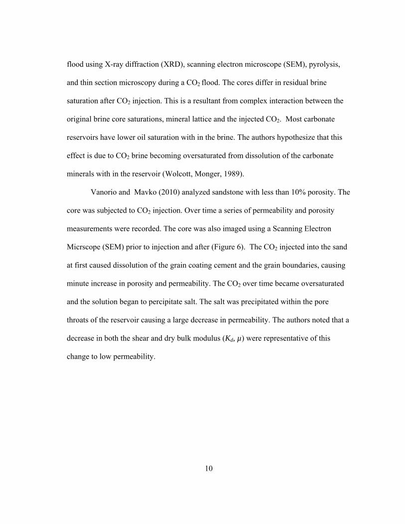
brine and reservoir minerals. ................................................................................ 8 Figure 6. SEM images of the core analyzed by Vanorio and Mavko (2010) with a

cross plot showing decrease in dry bulk modulus and shear modulus with more injected CO2 (Vanorio, Mavko, 2010) ...................................................... 11

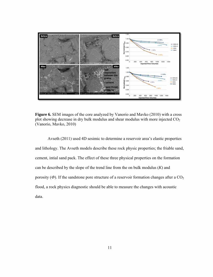
Figure 7. Two rock physics diagnostic of seismic which are able to determine the

geometrical grain structure between the cement and the matrix and the amount and type of cement as indicated by the color scale (Avseth 2011). ...... 12

Figure 8. Pore space compressibility versus porosity with respect to constant gamma

(Mammadova, 2011). ......................................................................................... 13 Figure 9. P and Shear-wave velocities against pressure plots for different pore

structure samples saturated with water, oil, CO2 gas and CO2 liquid respectively (Mammadova, 2011). .................................................................... 14

Figure 10. A schematic describing the process of the reflection coefficient

calculation. ......................................................................................................... 16 Figure 11. A schematic describing the process of the reflection coefficient

calculation. ......................................................................................................... 19 Figure 12. A graph displaying the usual change of the P-wave velocity with

increased confining pressure (Hoffman, Xu, 2005). .......................................... 22

ix

Figure 13. a) Is the transducer assembly used to measure Delhi core used for core

analysis at Oklahoma University. b) A schematic representation of a transducer assembly(Mohapatra, 2012). ............................................................ 24

Figure 14. A graph displaying the methodology of how to calculate n for a dynamic

reservoir(Hoffman, Xu, 2005). .......................................................................... 24 Figure 15. The Geometric interpretations of the Voigt and Reuss models (Mavko,

Mukerji, 2009) ................................................................................................... 28 Figure 16. Velocity measurements of different rock compositions and porosities with

the Voigt and Reuss limits and the Hill average trend line. (Mavko, Mukerji, 2009) ................................................................................................... 28

Figure 17. The Geometric interpretations of the time average method used for both

Wyllie (1958) and Raymer (1980) Models (Marko 2006). ................................ 30 Figure 18. A type log created from one of the original wells drilled in the Delhi

prospect. ............................................................................................................. 38 Figure 19. The Delhi Field represented by a bright green shape of the field and the

Jackson Dome CO2 Field represented by a CO2 gas well symbol. The red line is the Green Pipeline. The shadings represent possible different lithofacies. The bottom right picture is a cross-section of Louisiana from A to A’ (Eversull, 1985). ....................................................................................... 40

Figure 20. A burial chart of Mississippian Interior Salt Basin with the maturity levels

of any oil generation rom any organic layers. The units of this study are the Tuscaloosa and Paluxy Sandstone (Mancini and Puckett 2002). ...................... 41

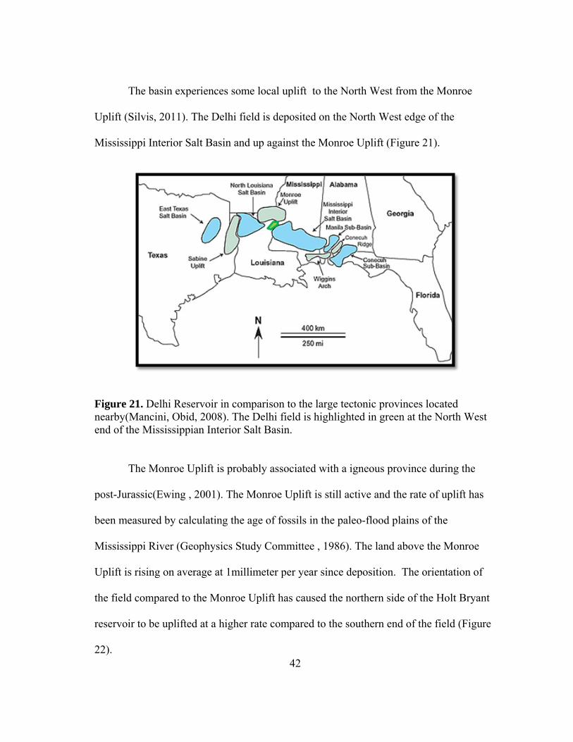
Figure 21. Delhi Reservoir in comparison to the large tectonic provinces located

nearby(Mancini, Obid, 2008). The Delhi field is highlighted in green at the North West end of the Mississippian Interior Salt Basin. .................................. 42

Figure 22. The structure Map of the continuous Clayton Lime in SSTVD (ft). The

yellow figure is the shape of the Delhi Field. The Clayton Lime is located right above the Holt Bryant Reservoir. And has a similar trend of sloping down to the southeast. The contour interval is 2000 ft. and the grid XY coordinates is in Township and Rang for North Louisiana. .............................. 43

x

Figure 23. Stratigraphic units and their relative units and ages. The units show very similar facie and sea level change as represented by the transgression and regression curve on the right. The upper teal box teal highlighted is the Tuscaloosa formation in the Holt-Bryant reservoir and the low red box highlighted is the Paluxy. The red lines represent the sea level trend during the Paluxy deposition and the teal line is the sea level trend for the Tuscaloosa (Mancini, Parcell, 1999). ................................................................ 44

Figure 24. The stratigraphy column around the region to the left and the Delhi

stratigraphy to the right. The formations of this research focus are highlighted in the red box. The most likely petroleum source is shown in the blue box (Nick Silvis modification from(Mancini, Parcell, 1999). ................... 46

Figure 25. The core description facie analysis correlated to the specific sand unit in

the Holt-Bryant Reservoir at well 159-2. The description of each facie can be seen in Table 2(Silvis 2011). ......................................................................... 50

Figure 26. Schmatic of a tidal dominated delta at the Gulf of Papua, Papua New

Guinea. The Tusc 1-8 is associated with the end of the delta, tidal sand bar. The Paluxy and Tusc 9 are associated with the beginning of the delta, delta plain/tidal flat (Society for Sedimentary Geology, 2013). ................................. 51

Figure 27. A general reconstruction of the depositional history of the Holt-Bryant

reservoir to the left. The upward arrow represents uplift created by the Monroe Uplift and the blue box is the oil water contact line. The present reservoir is to the right and the blue box represents the area of focus (Silvis, 2011). ................................................................................................................. 52

Figure 28. Schematic produced by Sun Oil Company showing the strong reflecting

layers below the Selma (Clayton Chalk) reflector. Depth in feet is on the Y axis and township and range sections are used for the above X axis. The Township and range for this diagram is T17N and R9E for Northern Louisiana (Hollingsworth, 1951). ...................................................................... 54

Figure 29. The reservoir limits and the 3 separate plays for the Holt-Bryant

Reservoir. Delhi-Blue; West Delhi-green, and Big Creek-red (Bloomer, 1946). ................................................................................................................. 55

Figure 30. Production history from Delhi. Y axis is in BPD or MCF/D and X axis is

in years. Before 1970 is a yearly average applied daily. Oil is the green line, Natural Gas is the red line, the dark blue is water injected and the light blue is water produced (Silvis, 2011). ....................................................................... 56

xi

Figure 31. Injection rate per day and bottom hole pressure of several test wells during the time of CO2 EOR production. The red line is the CO2 injection rate and it is related to the left axis. The blue dots are the different wells BHP and are related to the right axis. ................................................................ 58

Figure 32. Production of oil, gas (CO2 mostly), and water per day during the time of

CO2 EOR production. The red line is the gas production rate and it is related to the right axis. The green line is the oil production rate and the blue line is water production rate. Both are related to the left axis. ..................................... 59

Figure 33. Holt-Bryant reservoir net pay true vertical thickness (Hollingsworth,

1951). The red square is the RCP area. .............................................................. 60

Figure 34. RCP area at Delhi in the yellow square and their relation to the time lapsed seismic. ................................................................................................... 62

Figure 35. The research wells. The wells are 169-5, 159-2 and 140-1. The transparent

boxes are the different seismic acquisitions over the area. Dark blue is the 2009 data, teal is the 2010 and the green box is the 2011. For well 140-1 the 4-D seismic tie will have to be the 2011 data and not the 2010. ....................... 62

Figure 36. A Diagram showing the location of the three wells focused on in relation

to the production pattern used in the RCP area. Modified from(Silvis, 2011). ................................................................................................................. 63

Figure 37. Thin section samples showing typical mineralogy and pore structure of

the Paluxy sandstone. Thin section pictures and interpretations were done by Terry Eschner and Core Lab in July of 2009. ............................................... 65

Figure 38. A core description made by T. Eschner in 2010. The description from left

to right shows grain size, sedimentary structures, lithology, white light photo, UV photo, CT scan (showing structure), porosity and permeability. .... 66

Figure 39. A correlation between Patchy curves using the Biot-effective stress

variable (n) shown in Table 4. ........................................................................... 69 Figure 40: Cross plots comparing the log derived data at well 159-2 against the core

data. .................................................................................................................... 73 Figure 41. The crosssection shows the lithology, fluid saturation, and permeability of

the Holt-Bryant reservoir for the three wells which this research is focusing on. The key of the lithology is below the 159-2 well tracks and the location of the crossection is below the 169-5 well tracks. The lithology and fluid

xii

saturation is measured in percent and the permeability is measured in Darcy’s. .............................................................................................................. 74

Figure 42. The different phases of seismic during the history of the CO2 EOR flood at Delhi (Silvis, 2011). ....................................................................................... 76

Figure 43. The seismic fold over the Delhi region. The RCP area is in black. The

scale for fold is on the right. The increase in fold is due to overlap. ................. 77 Figure 44. An example of synthetic log from well 140-1 and 159-2. The same

lithology and fluid percent log as shown in Figure 4.9 is on the left track. The RC log is in the middle. The synthetic log is on the right track. The depth is measured depth and it is in feet. ........................................................... 78

Figure 45. The crosssection is a seismic profile of the 2008 data, inline 197. The

location of the crosssection is located in the map at the bottom, the green line is the Paluxy, teal is the Tuscaloosa and the grey line is the Clayton Chalk. ................................................................................................................. 79

Figure 46. A well tie between well 169-5 and the 2010 seismic data set. The green

lines are Paluxy, teal lines are Tuscaloosa, and grey line is the Clayton Chalk. The hashed lines are from the 2009 surface map. .................................. 80

Figure 47. An amplitude difference map between the Paluxy 2008 surface and the

Paluxy 2010 surface. The red areas imply positive amplitude change, blue areas imply negative amplitude change, and the grey areas imply no change. The yellow out line is the RCP area. The red triangles are injector wells and the green circles are the producing wells. .......................................................... 81

Figure 48. A cross-plot showing lithology associated with porosity in the Paluxy.

The area each lithology fills is the mineral percent composition (%Cn). .......... 87 Figure 49. A comparison between the permeability of the 169-5 well and the 159-2

well. The blue dots and line represent the 159-2 well and the green dots and line represent the 169-5 well. The line is a best fit exponential growth trend of the specific depth measurements of the log. .................................................. 88

Figure 50. Velocity and bulk modulus cross-plots against porosity for the wells 169-

4, 159-2 and 140-1. The actual data from the sonic log is the data points. Green points for 169-4, blue point for 159-2 and red points for 140-1. The rock physic models are the trend lines. Raymer (1980) in pink, Wyllie (1958) in orange, Hill in purple, Reuss in light purple and Voigt in dark purple. ................................................................................................................ 90

xiii

Figure 51. A comparison between the acoustic modulus of the 169-5 well and the

159-2 well. The left figure is the shear modulus with porosity and the right picture is the bulk modulus with porosity. The blue dots and line represent the 159-2 well and the green line and dots represent the 169-5 well. The line is a best fit exponential decay trend of the specific depth measurements of the log................................................................................................................. 91

Figure 52. A comparison between the dry bulk modulus calculated using

Gassmann’s (1998) model of the 169-5 well and the 159-2 well. The blue dots and line represent the 159-2 well and the green dots and line represent the 169-5 well. The line is a best fit exponential growth trend of the specific depth measurements of the log. ......................................................................... 93

Figure 53. A comparison between the Baechle (2005) ratio and porosity of the 169-5

well and the 159-2 well. The top graph is well 159-2 and the bottom graph is well 169-5. The symbols indicate type of porosity which is shown by thin sections to the left. Thin sections are from Terry Eschner 2009. ...................... 94

Figure 54. A comparison between the acoustic properties (shear and bulk modulus) with respect to porosity. The third dimension color represents the formation flexibility factor for the specific log data point on the graph. The trend lines are the same trend lines shown in figure 5.3. The red circle points out a pore property anomaly with the Paluxy in well 159-3. .............................................. 95

Figure 55. A cross-plot of lithology with porosity for both 2009 wells to show

similarity. ........................................................................................................... 97 Figure 56. A cross-plot of the Baechle (2005) ratio with porosity for both 2009 wells

to show similarity. .............................................................................................. 98 Figure 57. A cross-plot of the acoustic moduli with porosity and the framework

flexibility factor as the third color dimension for both 2009 wells to show similarity. ........................................................................................................... 98

Figure 58. A cross-plot of the shear moduli with porosity and dry bulk modulus with

porosity for both 2009 wells to show similarity. ............................................... 99 Figure 59. A synthetic using Petrel. The sonic and density logs used to calculate the

synthetic are on the left, the RC log is in the middle. The actual seismic acquired in 2011 surrounds the synthetic generated on the right track. ........... 100

xiv

Figure 60. The changes made to the bulk and shear modulus for the Paluxy formation in well 140-1 to match it better with the post CO2 interaction well 169-5. ..... 101

Figure 61. This figure shows the associated pore properties such as pore space bulk

modulus in Beaches’ (2005) ratio, and the Sun (2004) model framework flexibility factor. The trend lines shown in the two bottom cross-plots are done by using the new effective bulk and shear modulus. .............................. 102

Figure 62. A synthetic using Petrel. The sonic and density logs used to calculate the

synthetic are on the left, the RC log is in the middle. The actual seismic acquired in 2011 surrounds the synthetic generated on the right track. The new dry bulk synthetic is the left synthetic tie and the old dry bulk modulus from Figure 5.12 is to the right in the red box for comparison. ....................... 103

xv

LIST OF TABLES

Page Table 1. Some reservoir minerals and fluids with their associated average P-S wave velocity and density values. * indicates the material is not at STP (Mavko, Mukerji, 2009). ................................................................................................................................. 20 Table 2. Core analysis on the Holt-Bryant Core (Silvis, 2011) ....................................... 48 Table 3. Four porosity and mineralogy measurements for the Holt-Bryant core intervals at various depths. (XX## equals the SSTVD of the core in feet)(Mohapatra 2012). ................................................................................................................................. 67 Table 4. Measurements of n recorded during core analysis using multiple differential pressures(Mohapatra 2012). .............................................................................................. 68 Table 5. The minerals which are present in the core and their characteristics of certain log runs. The average values seen here are given by the Schlumberger 2010 Techlog Quanti Elan program. .......................................................................................... 71

1

1. INTRODUCTION

The societal standards the general public lives by today require cheap energy. In

the foreseeable future, the proper and efficient use of our domestic natural resources will

be crucial in sustaining the country’s economy. The Department of Energy (2011)

reported that 90% of the conventional wells in the United States are no longer

economical. Society relies on new methods of enhanced oil recovery (EOR) to keep our

modern way of living affordable.

Large volumes of domestic oil remain within reservoirs after conventional

primary production and secondary water flood. In most clastic sandstone reservoirs, an

average of 33-38% of the original oil in place (OOIP) can be produced after primary and

secondary recovery (Denbury, 2011). EOR techniques are used to increase the recovery

factor percentage of a reservoir past the primary and secondary production and are

crucial to keep fields at economical production rates. There are many types of EOR

techniques which are used today. This thesis focuses on the increasingly popular CO2

sequestration for EOR purposes.

The porosity of siliclastic rock may be predicted using mathematical models.

Gassmann (1998) and Sun’s (2004) equations are two of the models which can predict

porosity using acoustic properties of the reservoir rock. Porosity and permeability in

siliclastic rocks can change due to different pore geometries and diagenetic cement

texture during a CO2 flood. The purpose of this thesis is to measure any variations in

porosity and permeability using 3-D time lapsed seismic caused by a CO2 flood.

2

1.1 History of CO2 Sequestration

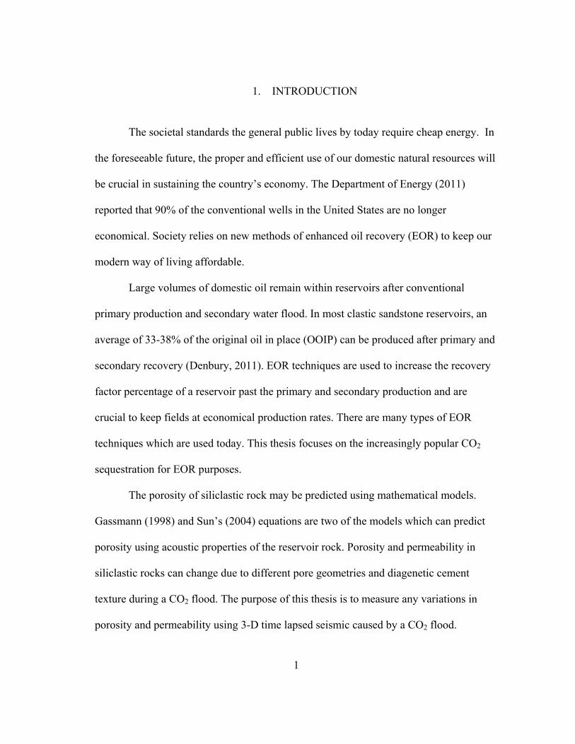
CO2 sequestration EOR has become very popular in recent years (EIA, 2011) for

a multitude of reasons (Figure 1). The following section will discuss the development of

this EOR technique and why it has become more economically viable.

Figure 1. Growth of CO2 produced of MMBO since 1972 (National Energy Technology Laboratory, 2010).

In 1952, Whorton and Brownscombe received a patent for an oil-recovery

method with CO2 through lab test on core data (Stalkup, 1978). In 1972, large

corporations began using the CO2 recovery method and reports from the Permian Basin

in Texas publicized successful EOR flooding of pilot test wells using CO2 as a

solvent(Brock and Bryan, 1989). In 1980 installation of CO2 pipelines in the Permian

3

basin began a revolution of CO2 EOR in Texas. Different techniques have been applied

during the process.

These different techniques include different injection processes, such as

continuous slug of water and gas, alternating between these two injection fluids (WAG),

and injecting pure CO2 in a supercritical state. There is also a variety of different

injection and production well patterns techniques. In some cases the injector is converted

to the producer. This is called a “huff n’ puff.”

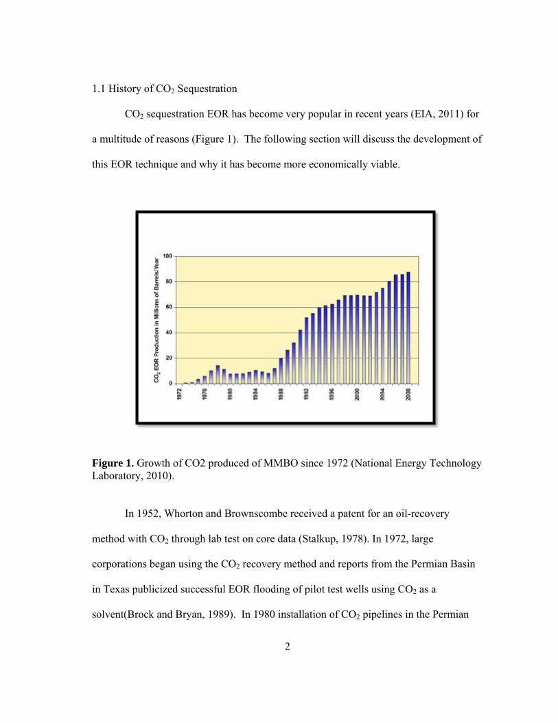
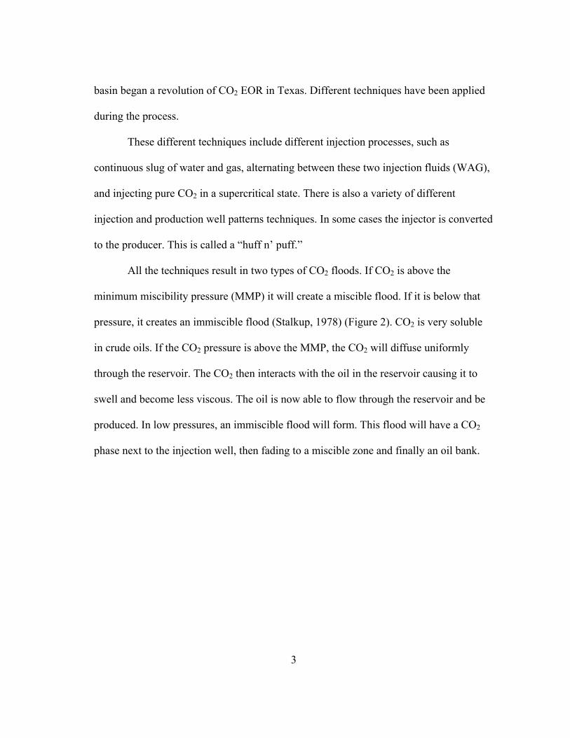
All the techniques result in two types of CO2 floods. If CO2 is above the

minimum miscibility pressure (MMP) it will create a miscible flood. If it is below that

pressure, it creates an immiscible flood (Stalkup, 1978) (Figure 2). CO2 is very soluble

in crude oils. If the CO2 pressure is above the MMP, the CO2 will diffuse uniformly

through the reservoir. The CO2 then interacts with the oil in the reservoir causing it to

swell and become less viscous. The oil is now able to flow through the reservoir and be

produced. In low pressures, an immiscible flood will form. This flood will have a CO2

phase next to the injection well, then fading to a miscible zone and finally an oil bank.

4

Figure 2. CO2 immiscible flood EOR (Denbury, 2011).

In July 2000, the Petroleum Technology Research Centre launched the

Weyburn CO2 Monitoring and Storage Project located in the Williston Basin with two

objectives. First, was to determine if CO2 could be sequestered securely in a reservoir. In

addition, they sought to determine the economic value of a CO2 EOR, including tax

incentives. This was mainly accomplished by using time lapsed seismic to monitor the

flow of CO2. During November 2005, Secretary Samuel W. Bodman announced that the

Department of Energy (DOE)-funded CO2 sequestration project was able to successfully

sequester five million tons of carbon dioxide while also doubling the recovery rate

5

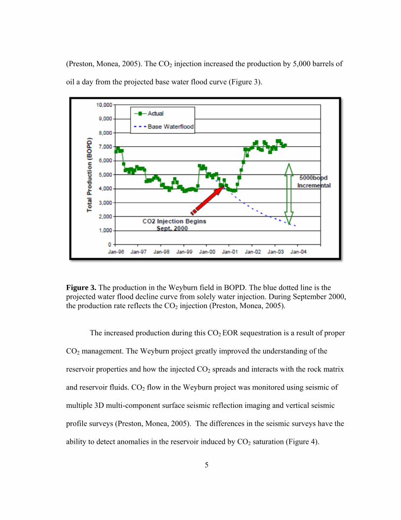
(Preston, Monea, 2005). The CO2 injection increased the production by 5,000 barrels of

oil a day from the projected base water flood curve (Figure 3).

Figure 3. The production in the Weyburn field in BOPD. The blue dotted line is the projected water flood decline curve from solely water injection. During September 2000, the production rate reflects the CO2 injection (Preston, Monea, 2005).

The increased production during this CO2 EOR sequestration is a result of proper

CO2 management. The Weyburn project greatly improved the understanding of the

reservoir properties and how the injected CO2 spreads and interacts with the rock matrix

and reservoir fluids. CO2 flow in the Weyburn project was monitored using seismic of

multiple 3D multi-component surface seismic reflection imaging and vertical seismic

profile surveys (Preston, Monea, 2005). The differences in the seismic surveys have the

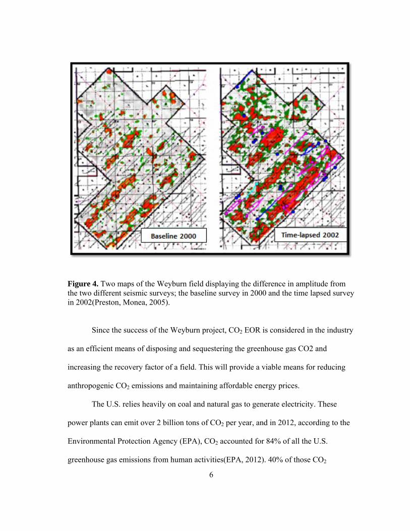
ability to detect anomalies in the reservoir induced by CO2 saturation (Figure 4).

6

Figure 4. Two maps of the Weyburn field displaying the difference in amplitude from the two different seismic surveys; the baseline survey in 2000 and the time lapsed survey in 2002(Preston, Monea, 2005).

Since the success of the Weyburn project, CO2 EOR is considered in the industry

as an efficient means of disposing and sequestering the greenhouse gas CO2 and

increasing the recovery factor of a field. This will provide a viable means for reducing

anthropogenic CO2 emissions and maintaining affordable energy prices.

The U.S. relies heavily on coal and natural gas to generate electricity. These

power plants can emit over 2 billion tons of CO2 per year, and in 2012, according to the

Environmental Protection Agency (EPA), CO2 accounted for 84% of all the U.S.

greenhouse gas emissions from human activities(EPA, 2012). 40% of those CO2

7

emissions are from power plants alone. On March 27, 2012, under the “Clean Air Act”,

the EPA limited the amount of carbon pollution that new power plants can emit which

will ensure that new facilities take advantage of clean technologies. For power plants to

be able to follow these new standards, carbon capture and CO2 sequestration

technologies must be employed. Many power plants are actively providing trapped CO2

to the many CO2 EOR companies in order to save the cost of in-house sequestration. If

this technique were applied at a world wide scale, CO2 emission may be cut in half over

the next 100 years(DOE, 2012).

CO2 flooding also revitalizes old oil fields. In the past century over a thousand

wells have been plugged and abandoned (P&A) during timFes of lenient, possibly

nonexistent laws. The CO2 EOR process will update these environmentally hazardous

P&A wells to recent standards(Warner and McConnell 1993). This process of CO2

capture and sequestration during an EOR flood is a highly efficient strategy for

producing our natural resources.

1.2 Statement of Problem

Recent research has suggested that CO2 will most likely cause permanent

diagenetic effects that will alter porosity and permeability. If the geochemical affects to

the porosity and permeability are not taken into account, an accurate assumption of

production or reservoir flood efficacy will not be possible. Using the mathematical

models provided by Gassmann (1998) and Sun (2004) the alterations of a reservoir could

possibly be measured and applied during production and CO2 flood simulations.

8

1.3 Importance

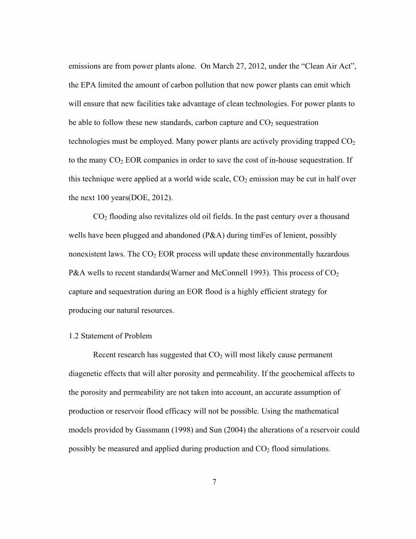
CO2 injected into brine solution creates the chemical reaction (Figure 5):

CO2 +H2O+Na(aq)+Cl(aq)= H2CO3 + NaCl

This reaction results in the products of carbonic acid (H2CO3) and salt (NaCl)(Vanorio,

Mavko, 2010). This reaction will induce digenesis that permanently changes the

reservoir. This includes dissolution of carbonates from the carbonic acid increasing

porosity, as well the precipitation of salt decreasing porosity.

Figure 5. Schematic the chemical interaction CO2 goes through with the aquifer brine and reservoir minerals.

9

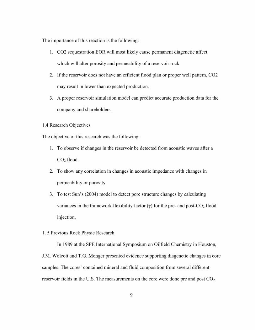
The importance of this reaction is the following:

1. CO2 sequestration EOR will most likely cause permanent diagenetic affect

which will alter porosity and permeability of a reservoir rock.

2. If the reservoir does not have an efficient flood plan or proper well pattern, CO2

may result in lower than expected production.

3. A proper reservoir simulation model can predict accurate production data for the

company and shareholders.

1.4 Research Objectives

The objective of this research was the following:

1. To observe if changes in the reservoir be detected from acoustic waves after a

CO2 flood.

2. To show any correlation in changes in acoustic impedance with changes in

permeability or porosity.

3. To test Sun’s (2004) model to detect pore structure changes by calculating

variances in the framework flexibility factor (γ) for the pre- and post-CO2 flood

injection.

1. 5 Previous Rock Physic Research

In 1989 at the SPE International Symposium on Oilfield Chemistry in Houston,

J.M. Wolcott and T.G. Monger presented evidence supporting diagenetic changes in core

samples. The cores’ contained mineral and fluid composition from several different

reservoir fields in the U.S. The measurements on the core were done pre and post CO2

10

flood using X-ray diffraction (XRD), scanning electron microscope (SEM), pyrolysis,

and thin section microscopy during a CO2 flood. The cores differ in residual brine

saturation after CO2 injection. This is a resultant from complex interaction between the

original brine core saturations, mineral lattice and the injected CO2. Most carbonate

reservoirs have lower oil saturation with in the brine. The authors hypothesize that this

effect is due to CO2 brine becoming oversaturated from dissolution of the carbonate

minerals with in the reservoir (Wolcott, Monger, 1989).

Vanorio and Mavko (2010) analyzed sandstone with less than 10% porosity. The

core was subjected to CO2 injection. Over time a series of permeability and porosity

measurements were recorded. The core was also imaged using a Scanning Electron

Micrscope (SEM) prior to injection and after (Figure 6). The CO2 injected into the sand

at first caused dissolution of the grain coating cement and the grain boundaries, causing

minute increase in porosity and permeability. The CO2 over time became oversaturated

and the solution began to percipitate salt. The salt was precipitated within the pore

throats of the reservoir causing a large decrease in permeability. The authors noted that a

decrease in both the shear and dry bulk modulus (Kd, µ) were representative of this

change to low permeability.

11

Figure 6. SEM images of the core analyzed by Vanorio and Mavko (2010) with a cross plot showing decrease in dry bulk modulus and shear modulus with more injected CO2 (Vanorio, Mavko, 2010)

Avseth (2011) used 4D sesimic to determine a reservoir area’s elastic properties

and lithology. The Avseth models describe these rock physic properties; the friable sand,

cement, intial sand pack. The effect of these three physical properties on the formation

can be described by the slope of the trend line from the on bulk modulus (K) and

porosity (Ф). If the sandstone pore structure of a reservoir formation changes after a CO2

flood, a rock physics diagnostic should be able to measure the changes with acoustic

data.

12

Figure 7. Two rock physics diagnostic of seismic which are able to determine the geometrical grain structure between the cement and the matrix and the amount and type of cement as indicated by the color scale (Avseth 2011).

Avseth shows the correlation between acoustic and pore structure properties is

not only applicable from well log data, but also 3-D seismic which spans the entire field

(Figure 7). Since both Sun (2004) and Aveseth’s (2011) models correlate dry bulk

modulus with the pore structure of a reservoir, possibly the Sun (2004) model maybe

applicable to the 3-D range as well.

Previous research done by Elnara Mammadova (2011) investigated the pore

structure changes caused by CO2 using Sun’s (2004) model. Mammadova injected

different fluids, including CO2, into core samples of a limestone reservoir under different

effective pressure scenarios. Carbonates are usually formations with complex pore

geometry which will alter locally. Because the reservoir is composed of almost all

carbonate minerals, the reservoir geometry will be subject to drastic changes during a

13

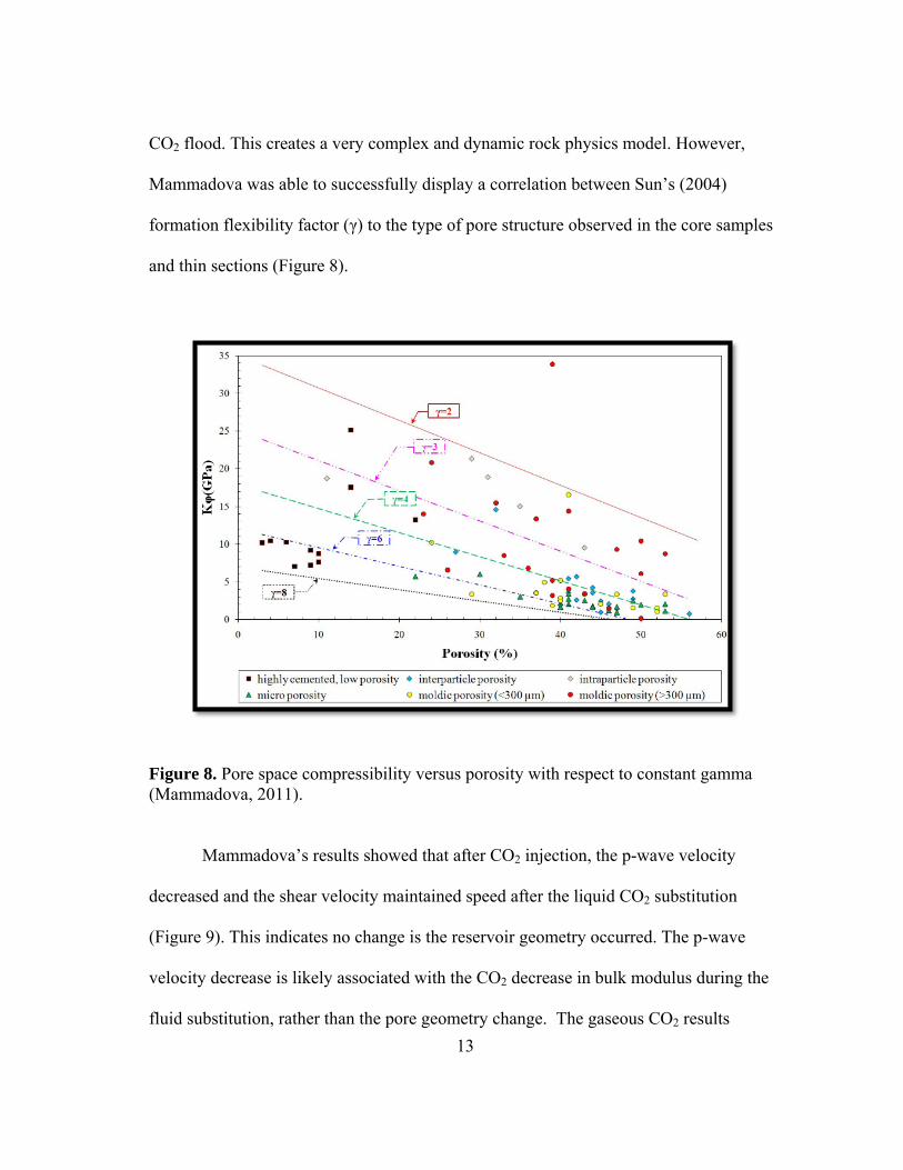
CO2 flood. This creates a very complex and dynamic rock physics model. However,

Mammadova was able to successfully display a correlation between Sun’s (2004)

formation flexibility factor (γ) to the type of pore structure observed in the core samples

and thin sections (Figure 8).

Figure 8. Pore space compressibility versus porosity with respect to constant gamma (Mammadova, 2011).

Mammadova’s results showed that after CO2 injection, the p-wave velocity

decreased and the shear velocity maintained speed after the liquid CO2 substitution

(Figure 9). This indicates no change is the reservoir geometry occurred. The p-wave

velocity decrease is likely associated with the CO2 decrease in bulk modulus during the

fluid substitution, rather than the pore geometry change. The gaseous CO2 results

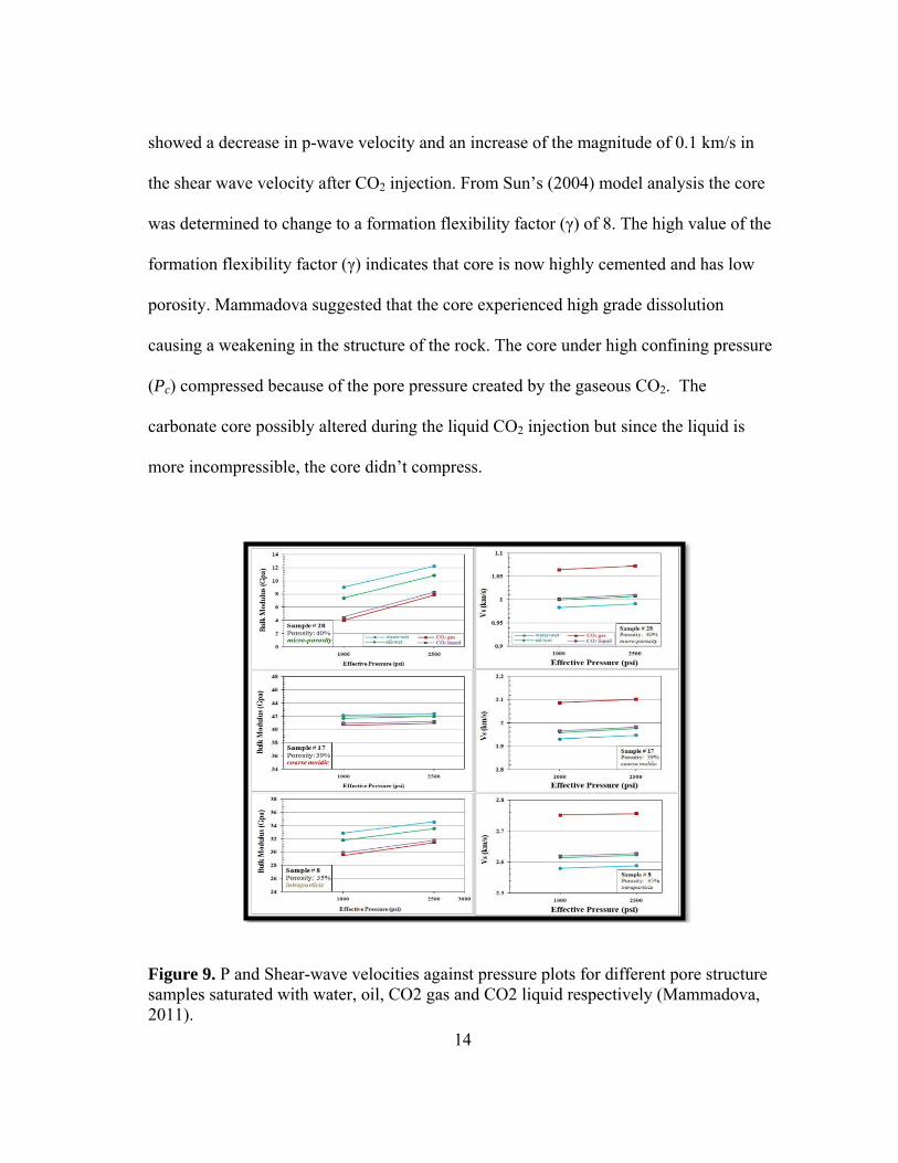
14

showed a decrease in p-wave velocity and an increase of the magnitude of 0.1 km/s in

the shear wave velocity after CO2 injection. From Sun’s (2004) model analysis the core

was determined to change to a formation flexibility factor (γ) of 8. The high value of the

formation flexibility factor (γ) indicates that core is now highly cemented and has low

porosity. Mammadova suggested that the core experienced high grade dissolution

causing a weakening in the structure of the rock. The core under high confining pressure

(Pc) compressed because of the pore pressure created by the gaseous CO2. The

carbonate core possibly altered during the liquid CO2 injection but since the liquid is

more incompressible, the core didn’t compress.

Figure 9. P and Shear-wave velocities against pressure plots for different pore structure samples saturated with water, oil, CO2 gas and CO2 liquid respectively (Mammadova, 2011).

15

A sandstone formation will have a dominant porosity that is interparticle, and

depending on the depositional setting, the pore geometry may stay consistent for large

areas of the reservoir. The Sun’s (2004) model formation flexibility factor (γ) range

should be relatively small. The matrix of sandstone is quartz which is non-reactive to

CO2. There may still be a diagenetic dissolution and compression of a sandstone

formation due to the dissolution of carbonate cement. Mammadova’s research provides

an insight on importance of an accurate prediction of the CO2 phase and elastic

properties during a fluid substitution model.

16

2. RESERVOIR ROCK PHYSIC MODELS

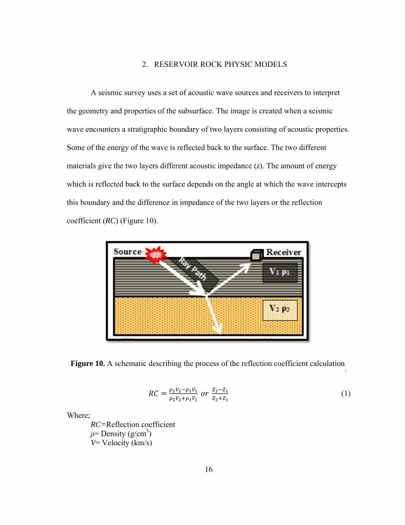
A seismic survey uses a set of acoustic wave sources and receivers to interpret

the geometry and properties of the subsurface. The image is created when a seismic

wave encounters a stratigraphic boundary of two layers consisting of acoustic properties.

Some of the energy of the wave is reflected back to the surface. The two different

materials give the two layers different acoustic impedance (z). The amount of energy

which is reflected back to the surface depends on the angle at which the wave intercepts

this boundary and the difference in impedance of the two layers or the reflection

coefficient (RC) (Figure 10).

Figure 10. A schematic describing the process of the reflection coefficient calculation.

𝑅𝐶 = 𝜌2𝑉2−𝜌1𝑉1𝜌2𝑉2+𝜌1𝑉1

𝑜𝑟 𝑍2−𝑍1𝑍2+𝑍1

(1)

Where; RC=Reflection coefficient ρ= Density (g/cm3) V= Velocity (km/s)

17

Z= Acoustic Impedance Using this formula a RC log can be derived using a density and sonic log (Ikelle

and Amundsen, 2005).Much like sonar, the sound waves travel time is used to create a

depth image by using the velocity of the subsurface and depth traveled to create a depth

image.

𝑡 = 2 ∗ 𝐷𝑉𝑝

(2)

2.1 Basic Overview of Seismic Wave Properties

At the acoustic source during seismic land surveys, multiple waves will be

produced with a variety of velocities. These waves include: air waves, surface (Rayleigh

and Love) waves, P-waves and S-waves. The waves which penetrate into the subsurface

are the elastic P and S waves. These waves are used during analysis of the subsurface

geometry and attributes.

P-waves are often referred to as the primary or pressure wave. This wave travels

through a series of molecule compression and refractions. The typical velocity for the P-

wave through a stratigraphic rock section is 5-8 km/s. The velocity depends on the

formations bulk (K) and shear (μ) Moduli properties. The bulk modulus is the rock

formation’s ability to resist any change in volume units of GPa and the shear modulus is

the rock’s formation’s ability to resist any change in shape units of GPa. The P-wave

velocity will cause both volume and shape change and is therefore calculated using both

moduli (EQ 3). S-waves are often referred to as secondary waves because their velocity

is always a magnitude slower than the P-wave velocity, as can be noticed by both

18

equations. These waves are also sometimes referred to as shear waves because the wave

only causes change in shape and is therefore calculated using only the shear moduli (4).

𝑉𝑝 = �𝐾𝑒+4 3� µ𝜌

(3)

𝑉µ = �µ𝜌 (4)

Where; V= P-Wave Velocity (km/s) K= Bulk Modulus (GPa) 𝜇= Shear Modulus (GPa)

Since fluid has theoretically has negligible resistance to shear change, the shear

modulus for all fluids will be considered 0 GPa and therefore the velocity of an S-wave

through a fluid will also be considered 0 km/s. There is still a debate in the scientific

community about the errors in this assumption (Baechle, Weger, 2005), but for this

research it will be considered valid.

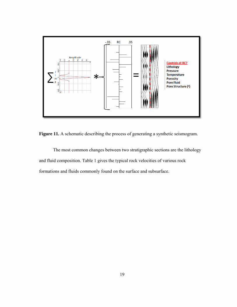
2.2 The Components of a Wave Reflection

The wave reflection image is created by a multiplication of a pulse wave by the

reflection coefficient (RC) at a boundary (EQ 1) (Figure 11). The RC is controlled by a

difference in a layers velocity and velocity is controlled by formation lithology, pressure,

temperature, porosity, pore fluid, and pore structure (EQ 3&4).

19

Figure 11. A schematic describing the process of generating a synthetic seismogram.

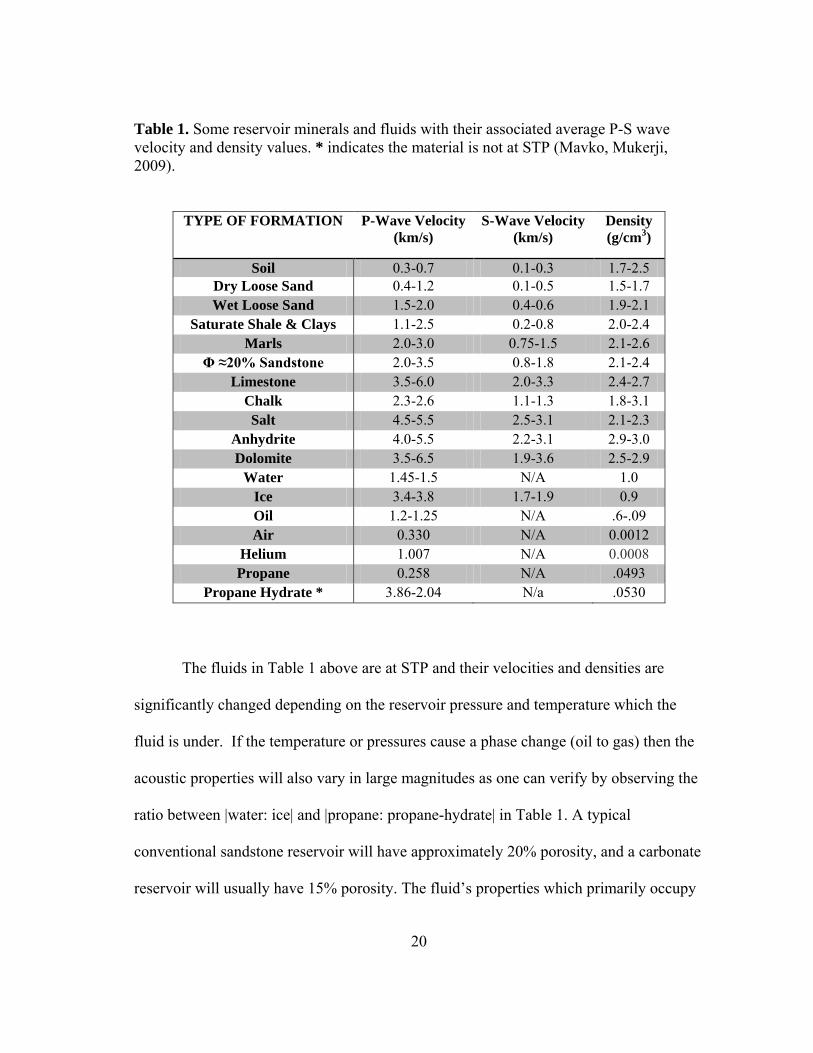
The most common changes between two stratigraphic sections are the lithology

and fluid composition. Table 1 gives the typical rock velocities of various rock

formations and fluids commonly found on the surface and subsurface.

20

Table 1. Some reservoir minerals and fluids with their associated average P-S wave velocity and density values. * indicates the material is not at STP (Mavko, Mukerji, 2009).

TYPE OF FORMATION P-Wave Velocity (km/s)

S-Wave Velocity (km/s)

Density (g/cm3)

Soil 0.3-0.7 0.1-0.3 1.7-2.5 Dry Loose Sand 0.4-1.2 0.1-0.5 1.5-1.7 Wet Loose Sand 1.5-2.0 0.4-0.6 1.9-2.1

Saturate Shale & Clays 1.1-2.5 0.2-0.8 2.0-2.4 Marls 2.0-3.0 0.75-1.5 2.1-2.6

Φ ≈20% Sandstone 2.0-3.5 0.8-1.8 2.1-2.4 Limestone 3.5-6.0 2.0-3.3 2.4-2.7

Chalk 2.3-2.6 1.1-1.3 1.8-3.1 Salt 4.5-5.5 2.5-3.1 2.1-2.3

Anhydrite 4.0-5.5 2.2-3.1 2.9-3.0 Dolomite 3.5-6.5 1.9-3.6 2.5-2.9

Water 1.45-1.5 N/A 1.0 Ice 3.4-3.8 1.7-1.9 0.9 Oil 1.2-1.25 N/A .6-.09 Air 0.330 N/A 0.0012

Helium 1.007 N/A 0.0008 Propane 0.258 N/A .0493

Propane Hydrate * 3.86-2.04 N/a .0530

The fluids in Table 1 above are at STP and their velocities and densities are

significantly changed depending on the reservoir pressure and temperature which the

fluid is under. If the temperature or pressures cause a phase change (oil to gas) then the

acoustic properties will also vary in large magnitudes as one can verify by observing the

ratio between |water: ice| and |propane: propane-hydrate| in Table 1. A typical

conventional sandstone reservoir will have approximately 20% porosity, and a carbonate

reservoir will usually have 15% porosity. The fluid’s properties which primarily occupy

21

the porosity will obviously drastically change the formation’s impedance. Therefore as

the reservoir fluid shifts from one dominant type to another, the resulting reflection

coefficient seen at the reservoir boundary will change as well. Understanding the fluid

properties of a reservoir is essential to any analysis of seismic data.

The effective pressure (Pe) of a reservoir is the difference between the confining

pressure (Pc) and the pore pressure (Pp) of a reservoir at the reservoir temperature (T).

𝑃𝑒 = 𝑃𝑐 − 𝑃𝑝 (5)

Where; n= the Biot Effective Stress Variable Pe= Effective Pressure (GPa) Pp= Pore Pressure (GPa)

The confining pressure is the compressional lithostatic pressure generated from

the surrounding rock. This pressure will stay consistent during a reservoirs production

lifetime. The pore pressure is the incompressible force created from the fluids within the

pore space of a reservoir rock. Any changes in a reservoir’s effective pressure are almost

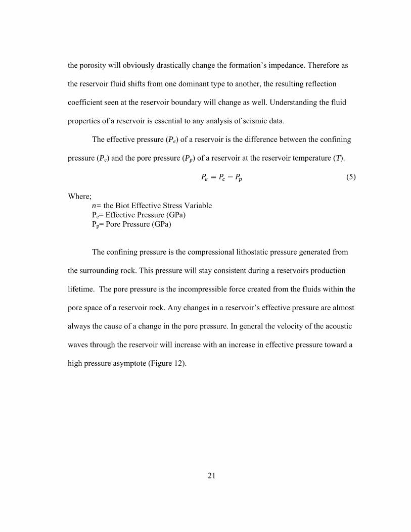
always the cause of a change in the pore pressure. In general the velocity of the acoustic

waves through the reservoir will increase with an increase in effective pressure toward a

high pressure asymptote (Figure 12).

22

Figure 12. A graph displaying the usual change of the P-wave velocity with increased confining pressure (Hoffman, Xu, 2005).

The equation for this research which will be used to define the reservoir fluid’s

bulk modulus is the Batzle (1992) dead oil (Ko), gas (Kg), and CO2 (KCO2) velocity

property model. Equation 8 is only used for CO2 which is in a reservoir at low pressure

and high temperature. This equation is referred to as the HTLP CO2 velocity model by

Batzle (1992) and is only valid is a reservoir with a formation pressure (Pe) between 7-

20 mega Pascal and temperature 25-200 degrees Celsius.

𝐾𝑔 = 𝑃𝑒�1−

𝑃𝑝𝑟𝑍 ∗ 𝛿𝑍

𝛿𝑃𝑝𝑟�𝑓(𝑇)

∗ 𝛼0 (6)

𝐾𝑂 = (15.450 ∗ (77.1 + 𝑂𝐴𝑃𝐼)−.5 − 3.7(𝑇) + 4.64(𝑃𝑒) + .0115�. 36 ∗ 𝑂𝐴𝑃𝐼 .5 − 1� ∗ 𝑇𝑃𝑒)2 ∗ 𝜌𝑂 (7)

𝐾𝐶𝑂2 = ⟨150 + 120 � 𝑇304.21

− 40(304.21−𝑇)304.21

� − �9 + 175 �1.5 − � 𝑇304.21

− 40(304.21−𝑇)304.21

���⟩2 𝑃𝑝𝑟 𝜌𝐶𝑂2 (8)

Where; 𝐾𝐹 = Fluid or Gas Bulk Moduli 𝜌𝐹 = Fluid or Gas Density Pe = Formation Pressure T = Temperature (Ko)

23

𝑃𝑝𝑟 = Pe / (Gas Critical Pressure) 𝛼0 = Ratio of Heat Capacity Z = Compressibility of Gas API = Specific Gravity of Oil

The calculation for the bulk modulus in water will be done at STP because the

changes in density and velocity offset each other with change in pressure. The velocity

of any water in the reservoir will have a velocity 1 km/s.

Pressure variations will not only change the fluid velocity and elastic properties,

but also the reservoir’s rock matrix properties as well. This is because the pressure

fluctuations will cause joints and pores within the reservoir to open or close. This

fluctuating porosity with pressure is referred to as soft porosity. The P-wave velocity is

largely affected by the amount of soft porosity within a rock because it accounts for

amount of fluid present. The S-Wave is not as drastically changed. The soft porosity can

be accounted for in the reservoir by the Biot effective stress coefficient (n).

𝑃𝑑 = 𝑃𝑐 − 𝑛𝑃𝑝 (𝑖𝑓 𝑛 = 1;𝑃𝑑 = 𝑃𝑒 = 𝑃𝑐 − 𝑃𝑝) (9)

Where; n= the Biot Effective Stress Variable Pd= Differential Pressure (GPa) Pe= Effective Pressure (GPa) Pp= Pore Pressure (GPa)

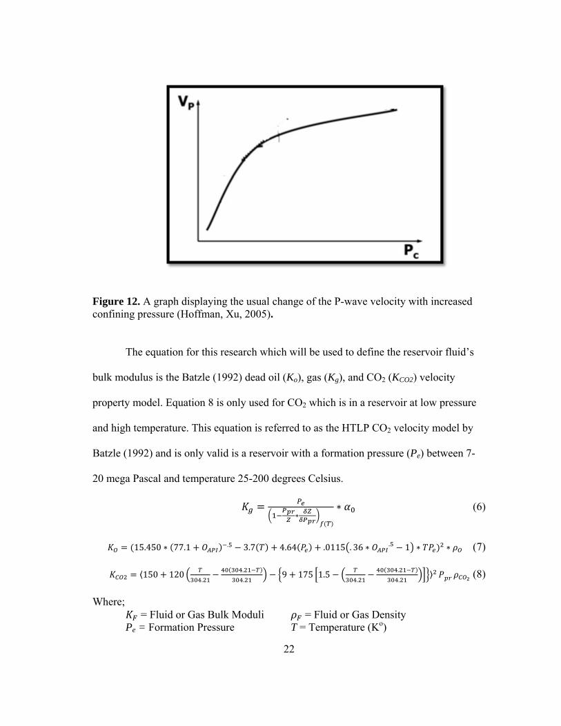
The only way to know rock’s matrix change to pressure is to physically measure

a core sample in a transducer assembly (Figure 13). This assembly allows lithostatic and

pore pressure to be held at various known constant values.

24

Figure 13. a) Is the transducer assembly used to measure Delhi core used for core analysis at Oklahoma University. b) A schematic representation of a transducer assembly(Mohapatra, 2012).

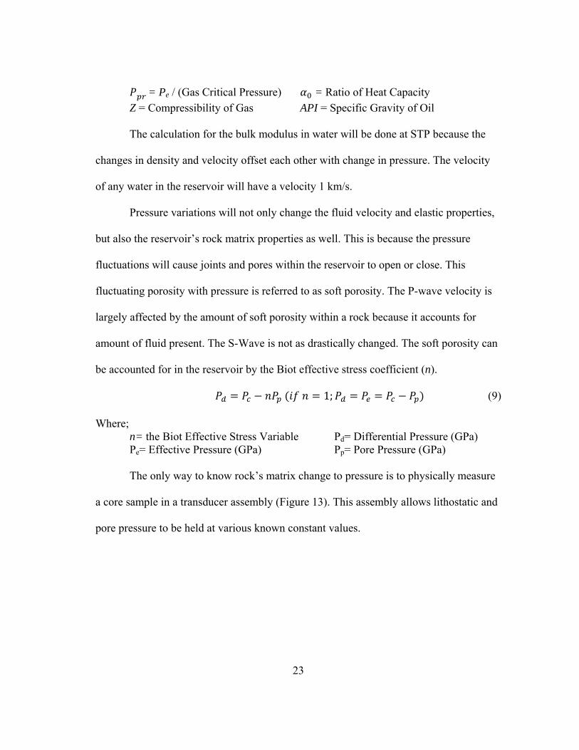
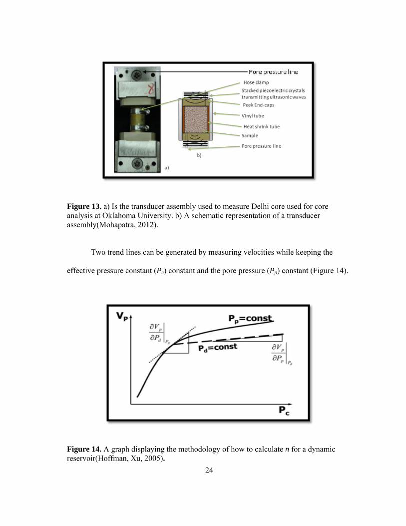
Two trend lines can be generated by measuring velocities while keeping the

effective pressure constant (Pe) constant and the pore pressure (Pp) constant (Figure 14).

Figure 14. A graph displaying the methodology of how to calculate n for a dynamic reservoir(Hoffman, Xu, 2005).

25

(ΔVp/ΔPp) is the slope of the dotted line. (ΔVp/ΔPe) is the tangent slope of the solid line at

the point where the two lines intersect. The Biot effective stress coefficient at the desired

Pc and Pp is derived from the slope of the (ΔVp/ΔPe) and (ΔVp/ΔPp).

𝑛 = 1 −�∆𝑉𝑝∆𝑃𝑝

�𝑃𝑑=𝑐𝑜𝑛𝑠𝑡.

�∆𝑉𝑝∆𝑃𝑑

�𝑃𝑝=𝑐𝑜𝑛𝑠𝑡.

(10)

Where; n= The Biot Effective Stress Variable Vp= Velocity (km/s) Pp= Pore Pressure (GPa) Pd= Differential Pressure (GPa)

The Biot effective stress coefficient (n) may also be solved without any changes

needed to be made to the reservoir pressure. In a static pressure reservoir the variable

may be defined as the following equation(Robin 1973).

𝑛 = 1 − 𝐾𝑑𝐾𝑚

(11)

Where; n= The Biot Effective Stress Variable Kd= The Dry Bulk Modulus (GPa) Km= The Mineral Bulk Modulus (GPa)

The variables of the dry bulk modulus (Kd) and mineral bulk modulus (Km) will

be discussed further. The dry bulk modulus (Kd) is directly related to the variable which

will be used to complete the objective of this research, pore structure or framework

flexibility factor (γ). The pore structure variable is the last attribute which affects the

reservoir rock’s acoustic properties. It is the geometrical structure of the minerals and

pore spaces. There are nearly no stratigraphic layers in the real world which are truly

homogenous or isotropic, including the Delhi reservoir. Fortunately, the Delhi reservoir

26

has been cored and processed using a transducer assembly to solve for the Biot effective

stress coefficient (n). These data points are provided by Mohapatra in (2012). These data

will be used instead of static reservoir model, which uses the dry bulk modulus (Kd)

variable. By using the core data the results will avoid any concurrency issues creating a

bias.

2.3 Methods for Estimating a Reservoir’s Elastic Properties

There has been a great focus to develop an accurate model to estimate a

reservoir’s elastic properties from only lithology, porosity, temperature and pressure

data. If the formation elastic properties, porosity, lithology, pressure and temperature are

known, the pore fluids and geometrical granular structure are the only other variables

which effect seismic. This research will focus on five models which estimate the

velocity (Vp) and effective bulk modulus (Ke) of a formation. The models will be used to

show the correlation between the log and acoustic data. These models will also help to

determine the acoustic properties of well without acoustic data.

Elastic modules are a very efficient method to tracking fluid flow with in a

dynamic reservoir formation. If assuming that the granular structure remains the same,

the fluid saturation in areas can be predicted from a seismic signal. However, the

geometric arrangement of each mineral is the most difficult variable to model and

predict. This variable can allows for a range of velocity and elastic values of formation

samples with similar mineralogy and porosity. The range of the formation velocity is

calculated by the upper and lower bounds of the Voigt and Reuss models. The Voigt

bound iso-strain model (VV & KV) is the upper bound and the Reuss iso-stress (VR & KR)

27

model is the lower bound. These bounds allow a definite bound and any data points

outside the bounds must either be faulty data or data incorrectly processed.

2.4 Voigt and Reuss Bounds

The Voigt and Reuss are easy to comprehend because the models are solely

based on the average acoustic properties of the percent composition of the material

present:

𝑋𝑣 = ∑𝑋1 ∗ %𝐶1 + 𝑋2 ∗ %𝐶2 + ⋯𝑋𝑛 ∗ %𝐶𝑛 (12)

𝑋𝑅 = ∑(𝑋1 ∗ %𝐶1)−1 + (𝑋2 ∗ %𝐶2)−1 + ⋯ (𝑋𝑛 ∗ %𝐶𝑛)−1 (13)

Where; 𝑋 = 𝑉 𝑜𝑟 𝐾

V= P-Wave Velocity (km/s) K= Bulk Modulus (GPa) %Cn= the percent of composition of the nth material Both formulas can be used to solve for a formation velocity (V) and bulk

modulus (K) limit with porosity. The average velocity (V) and bulk modulus (K) of

each material present (X) is multiplied by that materials percent composition (%C). The

Voigt model describes a reservoir composed of all materials vertically associated with

each other and the Reuss model is the inverse of the Voigt and describes a reservoir

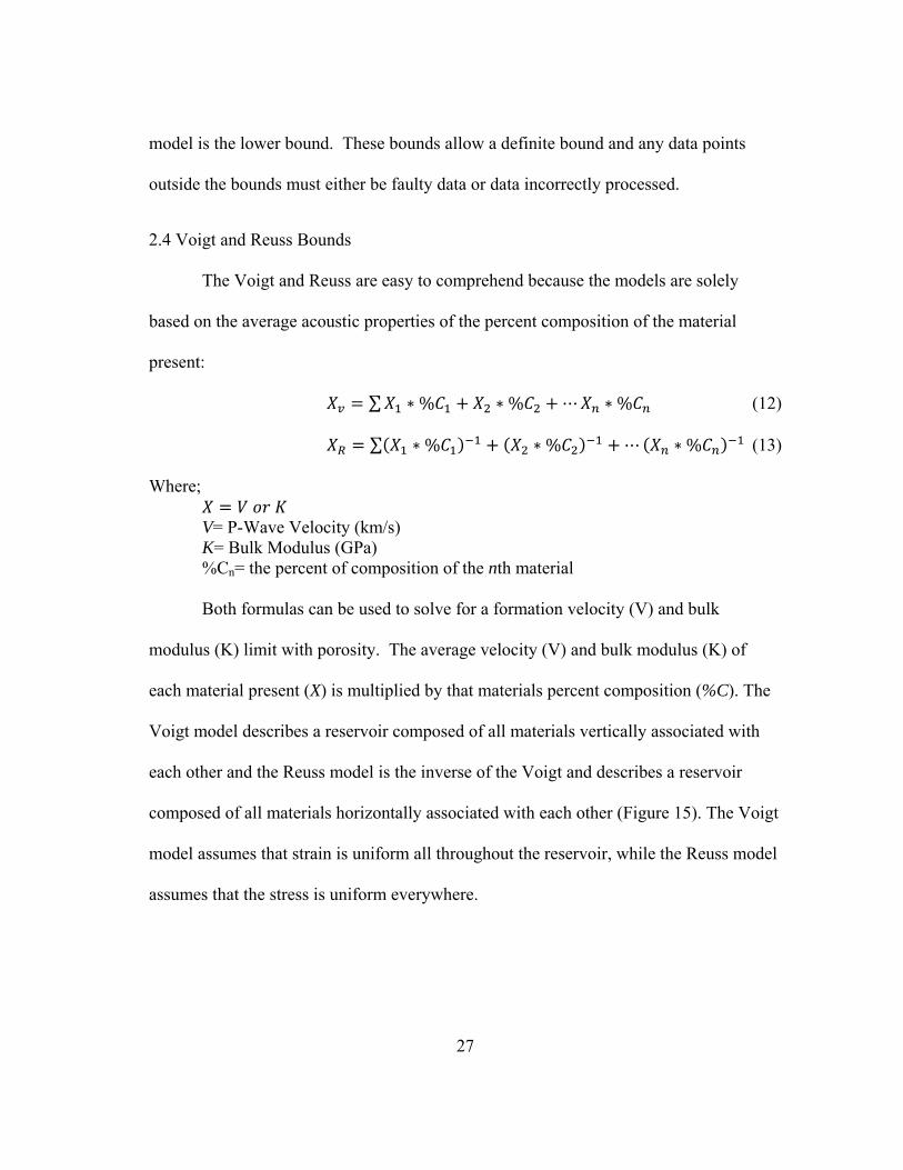
composed of all materials horizontally associated with each other (Figure 15). The Voigt

model assumes that strain is uniform all throughout the reservoir, while the Reuss model

assumes that the stress is uniform everywhere.

28

Figure 15. The Geometric interpretations of the Voigt and Reuss models (Mavko, Mukerji, 2009)

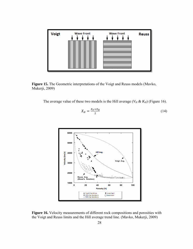
The average value of these two models is the Hill average (VH & KH) (Figure 16).

𝑋𝐻 = 𝑋𝑉+𝑋𝑅2

(14)

Figure 16. Velocity measurements of different rock compositions and porosities with the Voigt and Reuss limits and the Hill average trend line. (Mavko, Mukerji, 2009)

29

Note in Figure 16, the large variance in velocity measurements for rock samples

with similar lithology and porosity. The reason for this range is because of the varying

geometry of sand and clay grains. As the samples approach higher porosity and higher

percent fluids, the wave velocity trends with the lower limit Reuss model. This is

because the shear modulus of fluids is zero. In these models the p-wave velocity would

be the square root of bulk modulus of the formation (K) divided by the density of the

formation. This is because the shear modulus (μm) is approaching zero.

Baechle presented a new variable in 2005 which accounts for the variability in

velocity for formations which have similar lithology and saturation. This variable is

referred to as the pore stiffness ratio (kp), which is directly related to the ratio of pore

space bulk modulus (Kϕ) and the formation mineral modulus (Km). The range in the pore

stiffness ratio (kp) describes the formation’s dominant pore structure as either micro or

macro porosity. The higher ratio value indicates more micro-porosity.

𝑘𝑝 = 𝐾𝜙𝐾𝑚

(15)

Where; Kϕ=Pore Space Bulk Modulus (GPa) Km=Mineral Bulk Modulus (GPa) kp= The Pore Stiffness Ratio

The pore space bulk modulus (Kϕ) is the resistance the pore geometry of a

completely “dry” core sample. “Dry rock” is a theoretical fluid and gas drained rock.

The bulk modulus of the dry sample is simply referred to as the dry bulk modulus (Kd).

A saturated sample (Ke) will always yield a higher bulk modulus. To solve for both the

dry bulk modulus (Kd) and pore space bulk modulus (Kϕ), a core sample must be obtained

and completely drained of fluids. Then the acoustic properties of the core can be

30

measured under reservoir temperature and pressure. The relationship between both pore

space bulk moduli (Kϕ) the dry bulk moduli (Kd) is the following formula (Baechle,

Eberli, 2009)

1𝐾𝑑

= 𝜙𝐾𝜙

+ 1𝐾𝑚

(16)

Core analysis is very expensive, so other models have been made to best estimate these

variables.

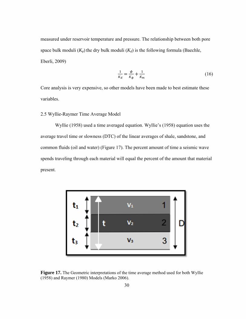
2.5 Wyllie-Raymer Time Average Model

Wyllie (1958) used a time averaged equation. Wyllie’s (1958) equation uses the

average travel time or slowness (DTC) of the linear averages of shale, sandstone, and

common fluids (oil and water) (Figure 17). The percent amount of time a seismic wave

spends traveling through each material will equal the percent of the amount that material

present.

Figure 17. The Geometric interpretations of the time average method used for both Wyllie (1958) and Raymer (1980) Models (Marko 2006).

31

𝑉 =𝐷∆𝑡

;𝐷 =𝑉∆𝑡

=𝑉1∆𝑡1

+𝑉2∆𝑡2

+𝑉3∆𝑡3

𝐷 = (%𝐶2 + %𝐶3 + 𝜙1);

𝜙1 =𝑉∆𝑡−%𝐶2−%𝐶3𝑉1∆𝑡1

−%𝐶2−%𝐶3 (17)

This is sometimes commonly referred to as a sonic porosity in logs. Since the

research will involve using the sonic properties to study the rock properties a different

method to calculate porosity will be used in order to avoid concurrency bias of using

similar data. If porosity is known, the equation can be re-written as the following.

𝐷∆𝑡

= 1𝑉

= 𝜙1𝑉1

+ (1−𝜙)𝑉2%𝐶2

+ (1−𝜙)𝑉3(%𝐶3)

(18)

Where; t= time (s) Φ= Porosity (%) V= P-Wave Velocity (km/s) %C1,2= Percent Composition (%) D= depth (km) Raymer in in 1980 modified Wyllie’s (1958) equation because the Wyllie (1958)

model is based on the ray theory which requires that the porosity to be large enough or

that the frequency of the wave to be high enough that the wavelength can fit into the

pore space. This large of porosity is highly unlikely in any reservoir formation. The

Raymer (1980) model is based on a best fit line created based on lab experimental data

with controlled lithology, fluids and porosity in a core sample. Raymer’s (1980)

experiments revealed that the mineralogy velocity (Vm) is related to the porosity fluids

by an exponent of two. Raymer (1980) associated this relation to the formation being

below 40% porosity and thus mineralogy interacts with more of the wave length.

32

𝑉 = (1 − 𝜙)2(𝑉2%𝐶2 + 𝑉3%𝐶3) + 𝜙1𝑉1 (19)

Where; t= time (s) Φ= Porosity (%) V= P-Wave Velocity (km/s) %C1,2= Percent Composition of (%) D= depth (km)

The examples of Wyllie (1958) and Raymer (1980) (EQ 16 & 17) shown above

are a highly simplified example only using shale and sand as the matrix. The research

formation will most likely have a much larger variance than two components. As with

the previous Voigt, Reuss, and Hill model, the shear modulus will only consider the

mineral data.

During this research, these models will be used to investigate the bulk modulus

(K), velocity (V), and the ratio between the bulk and shear modulus (K/μ) pre and post

CO2 flood to determine if the reservoir has experienced any rock physic changes as a

result from digenesis with the CO2. The model limitations are that the rock ideally needs

to be isotropic, high to medium effective formation pressure and have uniform fluid

saturation.

2.6 Biot-Gassmann Fluid Substitution and the Sun Model

The purpose of fluid substitution is to analyze how a seismic signal will

theoretically change with an associated fluid saturation change in order to predict the

recent fluid saturation only using modern seismic and old log data. The process requires

a synthetic seismogram to be made using log data. A synthetic seismic trace is generated

by multiplying a theoretical pulse generated at the surface by a Reflection Coefficient

(RC) log. The synthetic RC log can be generated using a predicted velocity and density

33

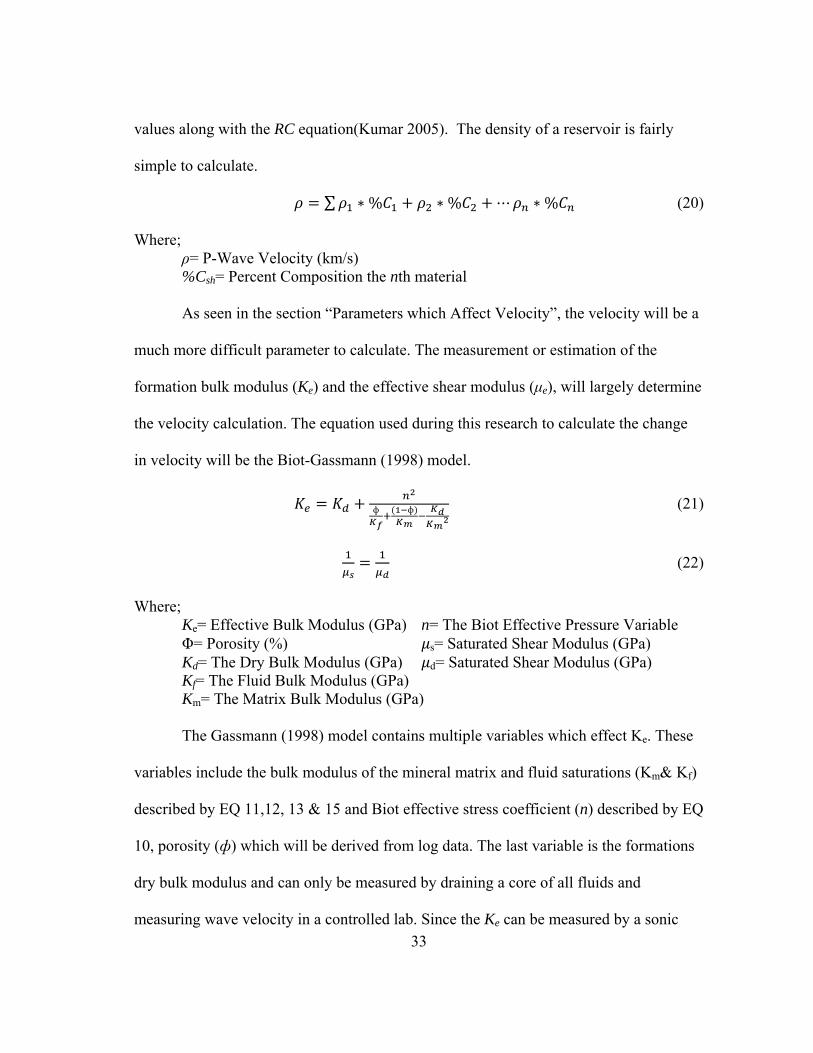
values along with the RC equation(Kumar 2005). The density of a reservoir is fairly

simple to calculate.

𝜌 = ∑𝜌1 ∗ %𝐶1 + 𝜌2 ∗ %𝐶2 + ⋯𝜌𝑛 ∗ %𝐶𝑛 (20)

Where; ρ= P-Wave Velocity (km/s) %Csh= Percent Composition the nth material As seen in the section “Parameters which Affect Velocity”, the velocity will be a

much more difficult parameter to calculate. The measurement or estimation of the

formation bulk modulus (Ke) and the effective shear modulus (μe), will largely determine

the velocity calculation. The equation used during this research to calculate the change

in velocity will be the Biot-Gassmann (1998) model.

𝐾𝑒 = 𝐾𝑑 + 𝑛2ф𝐾𝑓+(1−ф)

𝐾𝑚− 𝐾𝑑𝐾𝑚2

(21)

1𝜇𝑠

= 1𝜇𝑑

(22)

Where; Ke= Effective Bulk Modulus (GPa) n= The Biot Effective Pressure Variable Φ= Porosity (%) 𝜇s= Saturated Shear Modulus (GPa) Kd= The Dry Bulk Modulus (GPa) 𝜇d= Saturated Shear Modulus (GPa) Kf= The Fluid Bulk Modulus (GPa) Km= The Matrix Bulk Modulus (GPa) The Gassmann (1998) model contains multiple variables which effect Ke. These

variables include the bulk modulus of the mineral matrix and fluid saturations (Km& Kf)

described by EQ 11,12, 13 & 15 and Biot effective stress coefficient (n) described by EQ

10, porosity (ф) which will be derived from log data. The last variable is the formations

dry bulk modulus and can only be measured by draining a core of all fluids and

measuring wave velocity in a controlled lab. Since the Ke can be measured by a sonic

34

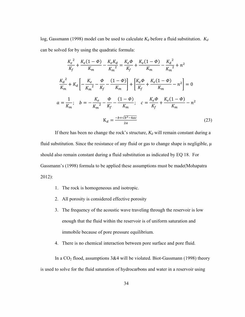
log, Gassmann (1998) model can be used to calculate Kd before a fluid substitution. Kd

can be solved for by using the quadratic formula:

𝐾𝑒2

𝐾𝑓+𝐾𝑒(1 − 𝛷)

𝐾𝑚−𝐾𝑒𝐾𝑑𝐾𝑚2 =

𝐾𝑒𝛷𝐾𝑓

+𝐾𝑒(1 − 𝛷)

𝐾𝑚−𝐾𝑑2

𝐾𝑚2 + 𝑛2

𝐾𝑑2

𝐾𝑚+ 𝐾𝑑 �−

𝐾𝑒𝐾𝑚2 −

𝛷𝐾𝑓

−(1 − 𝛷)𝐾𝑚

� + �𝐾𝑒𝛷𝐾𝑓

+𝐾𝑒(1 − 𝛷)

𝐾𝑚− 𝑛2� = 0

𝑎 =1𝐾𝑚

; 𝑏 = −𝐾𝑒𝐾𝑚2 −

𝛷𝐾𝑓

−(1 − 𝛷)𝐾𝑚

; 𝑐 =𝐾𝑒𝛷𝐾𝑓

+𝐾𝑒(1 − 𝛷)

𝐾𝑚− 𝑛2

K𝑑 = −𝑏+√𝑏2−4𝑎𝑐2𝑎

(23)

If there has been no change the rock’s structure, Kd will remain constant during a

fluid substitution. Since the resistance of any fluid or gas to change shape is negligible, μ

should also remain constant during a fluid substitution as indicated by EQ 18. For

Gassmann’s (1998) formula to be applied these assumptions must be made(Mohapatra

2012):

1. The rock is homogeneous and isotropic.

2. All porosity is considered effective porosity

3. The frequency of the acoustic wave traveling through the reservoir is low

enough that the fluid within the reservoir is of uniform saturation and

immobile because of pore pressure equilibrium.

4. There is no chemical interaction between pore surface and pore fluid.

In a CO2 flood, assumptions 3&4 will be violated. Biot-Gassmann (1998) theory

is used to solve for the fluid saturation of hydrocarbons and water in a reservoir using

35

seismic acoustic values. The module can be used to detect CO2 but not accurately predict

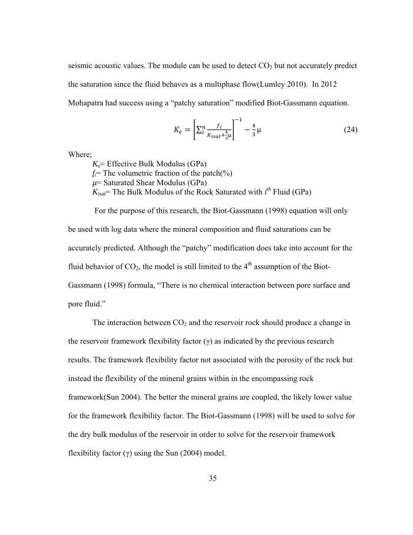
the saturation since the fluid behaves as a multiphase flow(Lumley 2010). In 2012

Mohapatra had success using a “patchy saturation” modified Biot-Gassmann equation.

𝐾𝑒 = �∑ 𝑓𝑖𝐾𝑖𝑠𝑎𝑡+

43µ

𝑛𝑖 �

−1

− 43µ (24)

Where; Ke= Effective Bulk Modulus (GPa) fi= The volumetric fraction of the patch(%) 𝜇= Saturated Shear Modulus (GPa) Kisat= The Bulk Modulus of the Rock Saturated with ith Fluid (GPa)

For the purpose of this research, the Biot-Gassmann (1998) equation will only

be used with log data where the mineral composition and fluid saturations can be

accurately predicted. Although the “patchy” modification does take into account for the

fluid behavior of CO2, the model is still limited to the 4th assumption of the Biot-

Gassmann (1998) formula, “There is no chemical interaction between pore surface and

pore fluid.”

The interaction between CO2 and the reservoir rock should produce a change in

the reservoir framework flexibility factor (γ) as indicated by the previous research

results. The framework flexibility factor not associated with the porosity of the rock but

instead the flexibility of the mineral grains within in the encompassing rock

framework(Sun 2004). The better the mineral grains are coupled, the likely lower value

for the framework flexibility factor. The Biot-Gassmann (1998) will be used to solve for

the dry bulk modulus of the reservoir in order to solve for the reservoir framework

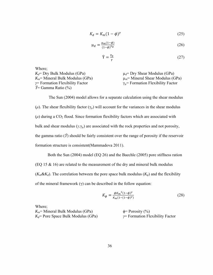
flexibility factor (γ) using the Sun (2004) model.

36

𝐾𝑑 = 𝐾𝑚(1 − 𝜙)𝛾 (25)

µ𝑑 = µ𝑚(1−𝜙)(1−𝜙)𝛾µ

(26)

Ῡ = 𝛾µ𝛾

(27)

Where; Kd= Dry Bulk Modulus (GPa) µd= Dry Shear Modulus (GPa) Km= Mineral Bulk Modulus (GPa) µm= Mineral Shear Modulus (GPa) γ= Formation Flexibility Factor γµ= Formation Flexibility Factor Ῡ= Gamma Ratio (%)

The Sun (2004) model allows for a separate calculation using the shear modulus

(μ). The shear flexibility factor (γµ) will account for the variances in the shear modulus

(μ) during a CO2 flood. Since formation flexibility factors which are associated with

bulk and shear modulus (γ,γµ) are associated with the rock properties and not porosity,

the gamma ratio (Ῡ) should be fairly consistent over the range of porosity if the reservoir

formation structure is consistent(Mammadova 2011).

Both the Sun (2004) model (EQ 26) and the Baechle (2005) pore stiffness ration

(EQ 15 & 16) are related to the measurement of the dry and mineral bulk modulus

(Km&Kd). The correlation between the pore space bulk modulus (Kϕ) and the flexibility

of the mineral framework (γ) can be described in the follow equation:

𝐾𝜙 = 𝜙𝐾𝑚2(1−𝜙)𝛾

𝐾𝑚(1−(1−𝜙)𝛾) (28)

Where; Km= Mineral Bulk Modulus (GPa) ϕ= Porosity (%) Kϕ= Pore Space Bulk Modulus (GPa) γ= Formation Flexibility Factor

37

This equation describes both the pore geometry and the mineral geometry for a

stratigraphic sedimentary unit. This research will investigate if any change can be

observed in these two factors after a CO2 injection.

38

3. AREA OF RESEARCH

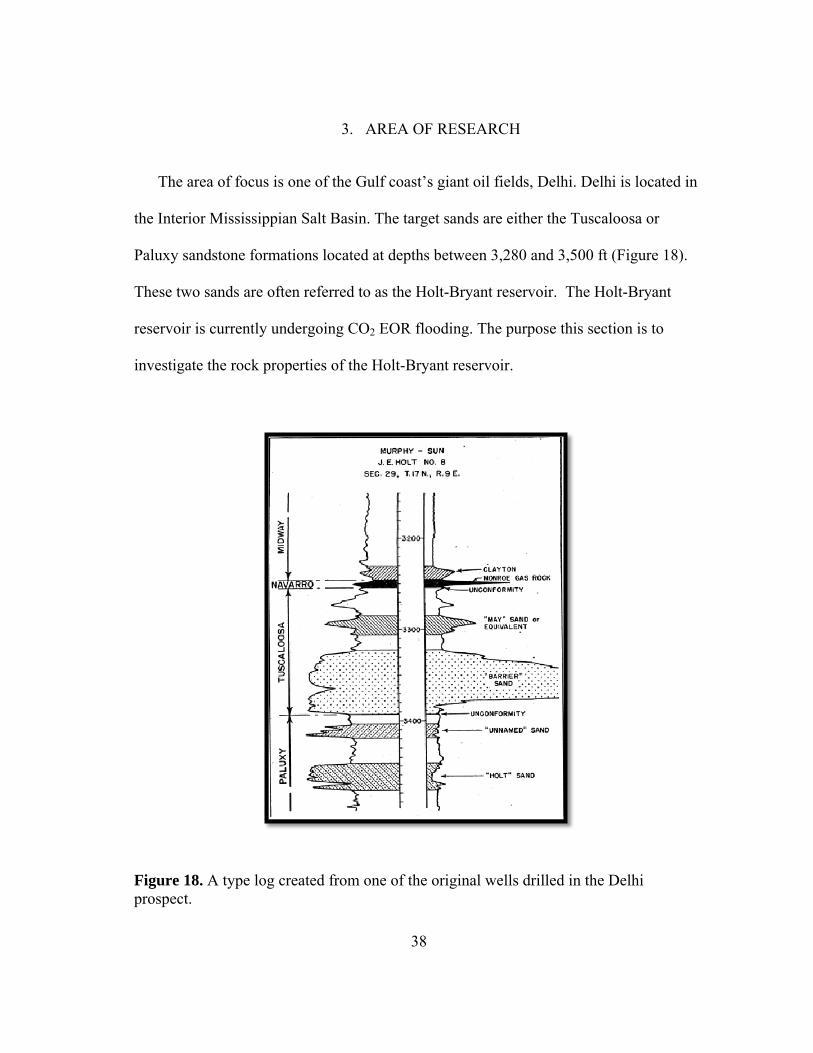
The area of focus is one of the Gulf coast’s giant oil fields, Delhi. Delhi is located in

the Interior Mississippian Salt Basin. The target sands are either the Tuscaloosa or

Paluxy sandstone formations located at depths between 3,280 and 3,500 ft (Figure 18).

These two sands are often referred to as the Holt-Bryant reservoir. The Holt-Bryant

reservoir is currently undergoing CO2 EOR flooding. The purpose this section is to

investigate the rock properties of the Holt-Bryant reservoir.

Figure 18. A type log created from one of the original wells drilled in the Delhi prospect.

39

3.1 Regional Geological Setting

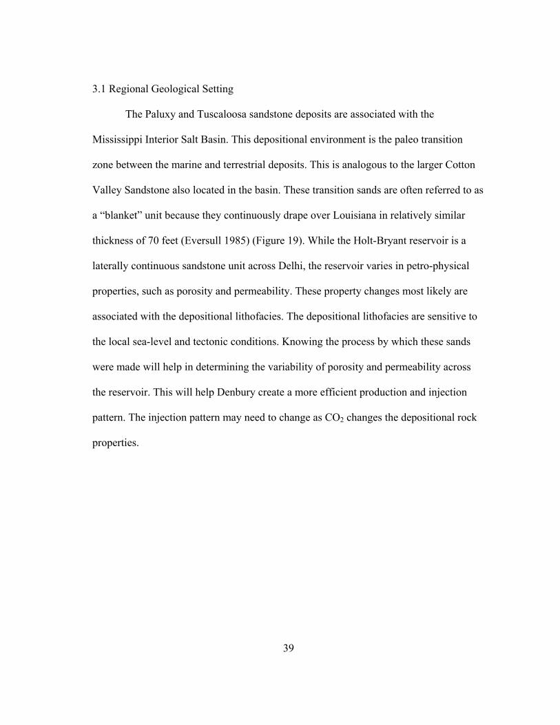
The Paluxy and Tuscaloosa sandstone deposits are associated with the

Mississippi Interior Salt Basin. This depositional environment is the paleo transition

zone between the marine and terrestrial deposits. This is analogous to the larger Cotton

Valley Sandstone also located in the basin. These transition sands are often referred to as

a “blanket” unit because they continuously drape over Louisiana in relatively similar

thickness of 70 feet (Eversull 1985) (Figure 19). While the Holt-Bryant reservoir is a

laterally continuous sandstone unit across Delhi, the reservoir varies in petro-physical

properties, such as porosity and permeability. These property changes most likely are

associated with the depositional lithofacies. The depositional lithofacies are sensitive to

the local sea-level and tectonic conditions. Knowing the process by which these sands

were made will help in determining the variability of porosity and permeability across

the reservoir. This will help Denbury create a more efficient production and injection

pattern. The injection pattern may need to change as CO2 changes the depositional rock

properties.

40

Figure 19. The Delhi Field represented by a bright green shape of the field and the Jackson Dome CO2 Field represented by a CO2 gas well symbol. The red line is the Green Pipeline. The shadings represent possible different lithofacies. The bottom right picture is a cross-section of Louisiana from A to A’ (Eversull, 1985).

The Mississippian Interior Salt Basin formed in the Late Triassic during the

rifting of Pangea. As the South American and African plates began to break away from

North America, the crust in the area began to thin through a process referred to as crustal

extension(Mancini, Obid, 2008). A sea floor spreading ridge formed in the Jurassic and

rifting continued. As the crust cooled, it became denser and subsided and formed the

present day basin of the Gulf of Mexico. At the time the climate was very arid with

shallow sea-levels. This allowed massive salt deposits to be formed, which are referred

to as the Louann Salt Sheets. Within the Gulf of Mexico are many sub basins including

the Mississippian Interior Salt Basin. Over time the basin has accumulated around

20,000 feet of sediment, and is the most oil and gas productive basin in the northeastern

41

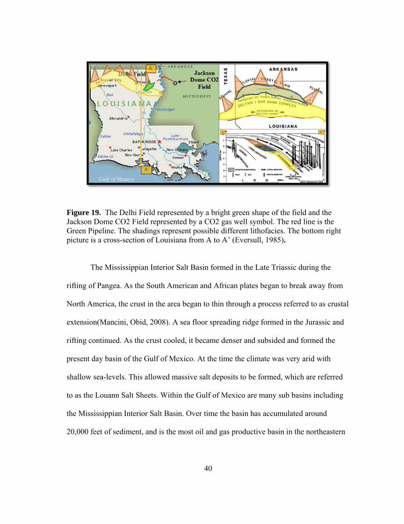
Gulf of Mexico, region producing over 2 billion barrels of oil and 6.3 trillion cubic feet

of natural gas (Mancini and Puckett 2002) (Figure 20).

Figure 20. A burial chart of Mississippian Interior Salt Basin with the maturity levels of any oil generation rom any organic layers. The units of this study are the Tuscaloosa and Paluxy Sandstone (Mancini and Puckett 2002).

42

The basin experiences some local uplift to the North West from the Monroe

Uplift (Silvis, 2011). The Delhi field is deposited on the North West edge of the

Mississippi Interior Salt Basin and up against the Monroe Uplift (Figure 21).

Figure 21. Delhi Reservoir in comparison to the large tectonic provinces located nearby(Mancini, Obid, 2008). The Delhi field is highlighted in green at the North West end of the Mississippian Interior Salt Basin.

The Monroe Uplift is probably associated with a igneous province during the

post-Jurassic(Ewing , 2001). The Monroe Uplift is still active and the rate of uplift has

been measured by calculating the age of fossils in the paleo-flood plains of the

Mississippi River (Geophysics Study Committee , 1986). The land above the Monroe

Uplift is rising on average at 1millimeter per year since deposition. The orientation of

the field compared to the Monroe Uplift has caused the northern side of the Holt Bryant

reservoir to be uplifted at a higher rate compared to the southern end of the field (Figure

22).

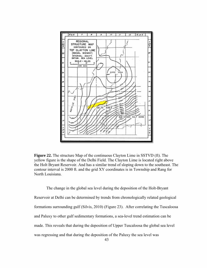
43

Figure 22. The structure Map of the continuous Clayton Lime in SSTVD (ft). The yellow figure is the shape of the Delhi Field. The Clayton Lime is located right above the Holt Bryant Reservoir. And has a similar trend of sloping down to the southeast. The contour interval is 2000 ft. and the grid XY coordinates is in Township and Rang for North Louisiana.

The change in the global sea level during the deposition of the Holt-Bryant

Reservoir at Delhi can be determined by trends from chronologically related geological

formations surrounding gulf (Silvis, 2010) (Figure 23). After correlating the Tuscaloosa

and Paluxy to other gulf sedimentary formations, a sea-level trend estimation can be

made. This reveals that during the deposition of Upper Tuscaloosa the global sea level

was regressing and that during the deposition of the Paluxy the sea level was

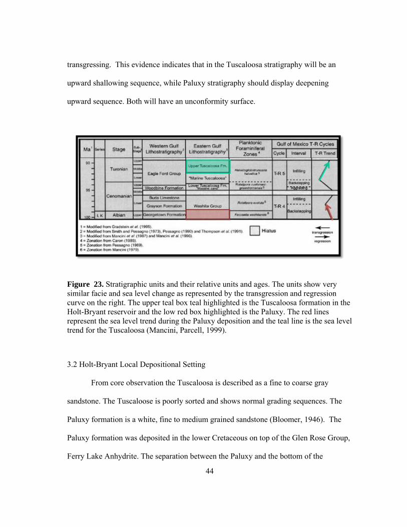
44

transgressing. This evidence indicates that in the Tuscaloosa stratigraphy will be an

upward shallowing sequence, while Paluxy stratigraphy should display deepening

upward sequence. Both will have an unconformity surface.

Figure 23. Stratigraphic units and their relative units and ages. The units show very similar facie and sea level change as represented by the transgression and regression curve on the right. The upper teal box teal highlighted is the Tuscaloosa formation in the Holt-Bryant reservoir and the low red box highlighted is the Paluxy. The red lines represent the sea level trend during the Paluxy deposition and the teal line is the sea level trend for the Tuscaloosa (Mancini, Parcell, 1999).

3.2 Holt-Bryant Local Depositional Setting

From core observation the Tuscaloosa is described as a fine to coarse gray

sandstone. The Tuscaloose is poorly sorted and shows normal grading sequences. The

Paluxy formation is a white, fine to medium grained sandstone (Bloomer, 1946). The

Paluxy formation was deposited in the lower Cretaceous on top of the Glen Rose Group,

Ferry Lake Anhydrite. The separation between the Paluxy and the bottom of the

45

Tuscaloosa is a small angular unconformity. The Tuscaloosa at Delhi can be separated

into nine sub-units with Tusc-1 being the lowest (Figure 24). These nine units are not

continuous across the Delhi Reservoir. Instead these units are lenses of sand local

present in areas around the reservoir. A major angular unconformity is above the

Tuscaloosa. The Monroe Gas Rock (MGR) is above the Tuscaloosa and then Clayton

Chalk. The Monroe and Clayton Chalk are both carbonate rocks. The Monroe Gas Rock

is a discontinuous unit which is at maximum 10 feet thick at Delhi. The Clayton Chalk is

a fine grained carbonate chalk which is continuously 10 feet across the reservoir and

serves as the seal. The overburden rock above the Clayton Chalk is the Midway Shale.

This shale is on average 500 feet thick at Delhi and it serves as a secondary seal. The

Jurassic Smackover is most likely the source rock in this play, although there has been

no geochemical correlation proving so (Mancini, Parcell, 1999).

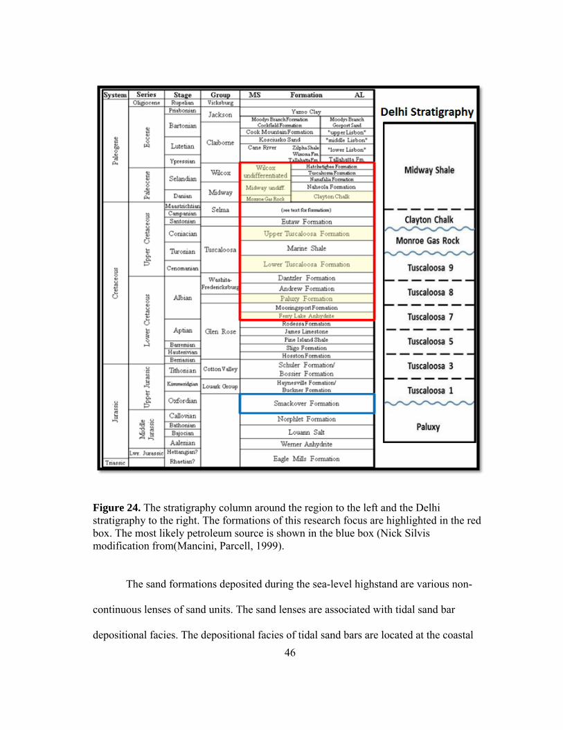
46

Figure 24. The stratigraphy column around the region to the left and the Delhi stratigraphy to the right. The formations of this research focus are highlighted in the red box. The most likely petroleum source is shown in the blue box (Nick Silvis modification from(Mancini, Parcell, 1999).

The sand formations deposited during the sea-level highstand are various non-

continuous lenses of sand units. The sand lenses are associated with tidal sand bar

depositional facies. The depositional facies of tidal sand bars are located at the coastal

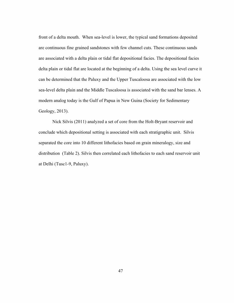
47

front of a delta mouth. When sea-level is lower, the typical sand formations deposited

are continuous fine grained sandstones with few channel cuts. These continuous sands

are associated with a delta plain or tidal flat depositional facies. The depositional facies

delta plain or tidal flat are located at the beginning of a delta. Using the sea level curve it

can be determined that the Paluxy and the Upper Tuscaloosa are associated with the low

sea-level delta plain and the Middle Tuscaloosa is associated with the sand bar lenses. A

modern analog today is the Gulf of Papua in New Guina (Society for Sedimentary

Geology, 2013).

Nick Silvis (2011) analyzed a set of core from the Holt-Bryant reservoir and

conclude which depositional setting is associated with each stratigraphic unit. Silvis

separated the core into 10 different lithofacies based on grain mineralogy, size and

distribution (Table 2). Silvis then correlated each lithofacies to each sand reservoir unit

at Delhi (Tusc1-9, Paluxy).

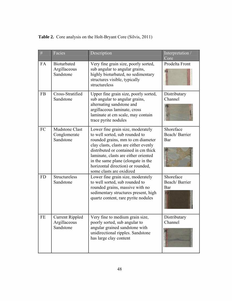
48

Table 2. Core analysis on the Holt-Bryant Core (Silvis, 2011)

# Facies Description Interpretation / Core

FA Bioturbated Argillaceous Sandstone

Very fine grain size, poorly sorted, sub angular to angular grains, highly bioturbated, no sedimentary structures visible, typically structureless

Prodelta Front

FB Cross-Stratified

Sandstone Upper fine grain size, poorly sorted, sub angular to angular grains, alternating sandstone and argillaceous laminate, cross laminate at cm scale, may contain trace pyrite nodules

Distributary Channel

FC Mudstone Clast

Conglomerate Sandstone

Lower fine grain size, moderately to well sorted, sub rounded to rounded grains, mm to cm diameter clay clasts, clasts are either evenly distributed or contained in cm thick laminate, clasts are either oriented in the same plane (elongate in the horizontal direction) or rounded, some clasts are oxidized

Shoreface Beach/ Barrier Bar

FD Structureless

Sandstone Lower fine grain size, moderately to well sorted, sub rounded to rounded grains, massive with no sedimentary structures present, high quartz content, rare pyrite nodules

Shoreface Beach/ Barrier Bar

FE Current Rippled Argillaceous Sandstone

Very fine to medium grain size, poorly sorted, sub angular to angular grained sandstone with unidirectional ripples. Sandstone has large clay content

Distributary Channel

49

Table 2. Continued

# Facies Description Interpretation / Core

FF Horizontally Laminated Argillaceous Sandstone

Very fine grain size, poorly sorted, sub angular to angular grains, horizontally laminated clay and sandstone, possible mm scale current ripples, organic matter

Delta Plain

FG Argillaceous Sandstone

Very fine grain size, poorly sorted, angular to sub angular grains, possible root traces, high clay content

Delta Plain

FH Oxidized

Mudstone Dark reddish color, plastic Delta Plain

FI Anoxic

Mudstone Light to dark gray color, plastic, in places contains mm scale fine sandstone laminate, sometimes bioturbated

Salt Marsh/ Lagoon

FJ Cross-Stratified

Sandstone with Mudclast Laminae

Upper fine grain size, poorly sorted, sub angular to angular grains, alternating sandstone and argillaceous laminate, cross laminate at cm scale, may contain trace pyrite nodules

Shoreface Beach/ Barrier Bar

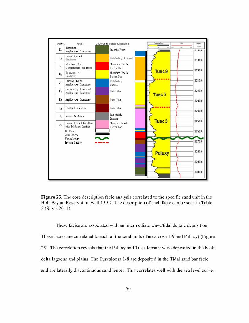
50

Figure 25. The core description facie analysis correlated to the specific sand unit in the Holt-Bryant Reservoir at well 159-2. The description of each facie can be seen in Table 2 (Silvis 2011).

These facies are associated with an intermediate wave/tidal deltaic deposition.

These facies are correlated to each of the sand units (Tuscaloosa 1-9 and Paluxy) (Figure

25). The correlation reveals that the Paluxy and Tuscaloosa 9 were deposited in the back

delta lagoons and plains. The Tuscaloosa 1-8 are deposited in the Tidal sand bar facie

and are laterally discontinuous sand lenses. This correlates well with the sea level curve.

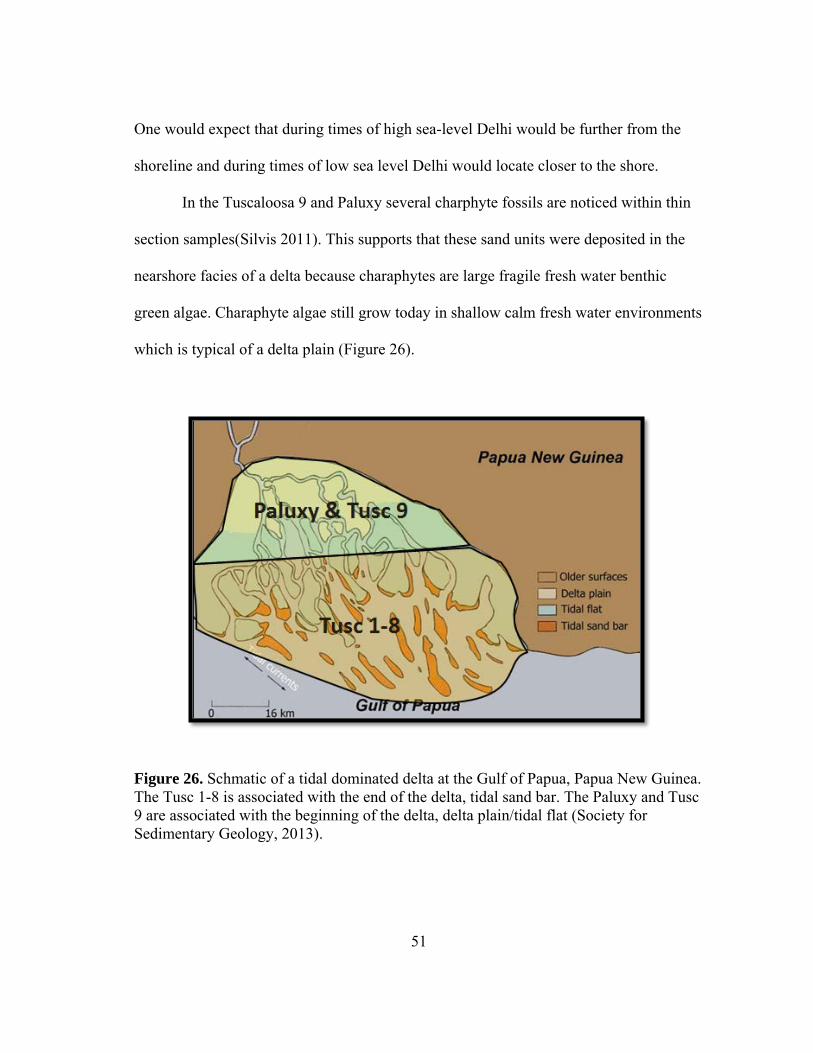
51

One would expect that during times of high sea-level Delhi would be further from the

shoreline and during times of low sea level Delhi would locate closer to the shore.

In the Tuscaloosa 9 and Paluxy several charphyte fossils are noticed within thin

section samples(Silvis 2011). This supports that these sand units were deposited in the

nearshore facies of a delta because charaphytes are large fragile fresh water benthic

green algae. Charaphyte algae still grow today in shallow calm fresh water environments

which is typical of a delta plain (Figure 26).

Figure 26. Schmatic of a tidal dominated delta at the Gulf of Papua, Papua New Guinea. The Tusc 1-8 is associated with the end of the delta, tidal sand bar. The Paluxy and Tusc 9 are associated with the beginning of the delta, delta plain/tidal flat (Society for Sedimentary Geology, 2013).

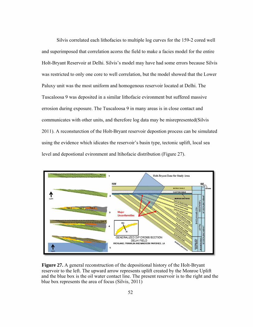
52

Silvis correlated each lithofacies to multiple log curves for the 159-2 cored well

and superimposed that correlation acorss the field to make a facies model for the entire

Holt-Bryant Reservoir at Delhi. Silvis’s model may have had some errors because Silvis

was restricted to only one core to well correlation, but the model showed that the Lower

Paluxy unit was the most uniform and homogenous reservoir located at Delhi. The

Tuscaloosa 9 was deposited in a similar lithofacie evironment but suffered massive

errosion during exposure. The Tuscaloosa 9 in many areas is in close contact and

communicates with other units, and therefore log data may be misrepresented(Silvis

2011). A reconsturction of the Holt-Bryant reservoir depostion process can be simulated

using the evidence which idicates the reservoir’s basin type, tectonic uplift, local sea

level and depostional evironment and ltihofacie distribution (Figure 27).

blue box represents the area of focus (Silvis, 2011)

Figure 27. A general reconstruction of the depositional history of the Holt-Bryant reservoir to the left. The upward arrow represents uplift created by the Monroe Uplift

and the blue box is the oil water contact line. The present reservoir is to the right and the

53

Since the Paluxy unit is the most homogenous and consistent unit in the Delhi

field, it will be the focus when applying any rock physics models to detect diagenetic

changes. The reason for this is because any well drilled pre-CO2 needs to comparable to

any post-CO2 drilled well without original differences.

3.3 Holt-Bryant Reservoir Structure

During the initial exploration, Sun Oil Company expanded around the reservoir

area and drilled a few dry wells toward the northern end of the field in the 1940’s. This

suggest the Holt-Bryant reservoir being some sort of structural trap. A seismic survey

was performed in order to further help Sun Oil in their well placement efficacy (Figure

28). The survey revealed that the Holt-Bryant reservoir sands are truncated by the

Midway Clayton Chalk. The truncation runs parallel with the current shoreline

(Hollingsworth, 1951). This unconformity is the structural trap which allowed collection

over time of hydrocarbons.

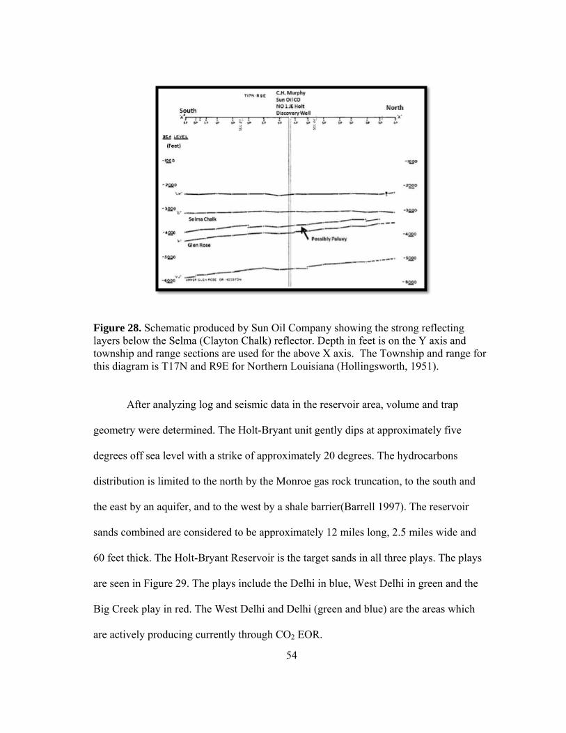
54

Figure 28. Schematic produced by Sun Oil Company showing the strong reflecting layers below the Selma (Clayton Chalk) reflector. Depth in feet is on the Y axis and township and range sections are used for the above X axis. The Township and range for this diagram is T17N and R9E for Northern Louisiana (Hollingsworth, 1951).

After analyzing log and seismic data in the reservoir area, volume and trap

geometry were determined. The Holt-Bryant unit gently dips at approximately five

degrees off sea level with a strike of approximately 20 degrees. The hydrocarbons

distribution is limited to the north by the Monroe gas rock truncation, to the south and

the east by an aquifer, and to the west by a shale barrier(Barrell 1997). The reservoir

sands combined are considered to be approximately 12 miles long, 2.5 miles wide and

60 feet thick. The Holt-Bryant Reservoir is the target sands in all three plays. The plays

are seen in Figure 29. The plays include the Delhi in blue, West Delhi in green and the

Big Creek play in red. The West Delhi and Delhi (green and blue) are the areas which

are actively producing currently through CO2 EOR.

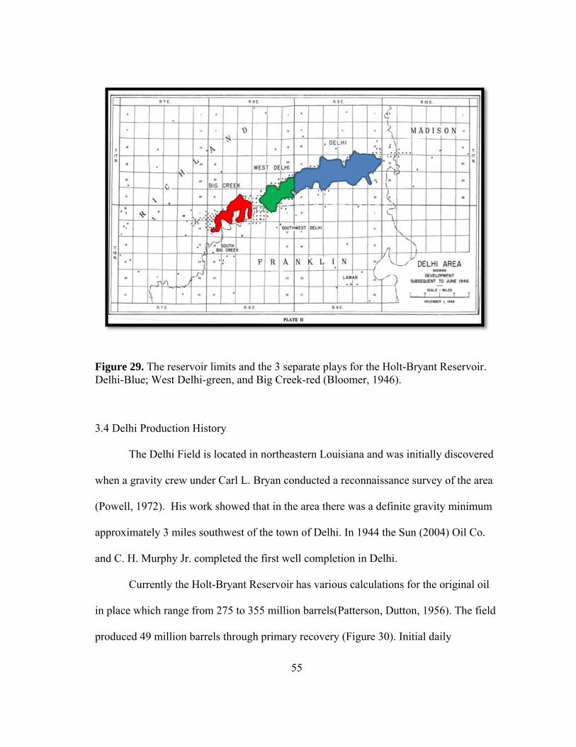
55

Figure 29. The reservoir limits and the 3 separate plays for the Holt-Bryant Reservoir. Delhi-Blue; West Delhi-green, and Big Creek-red (Bloomer, 1946).

3.4 Delhi Production History

The Delhi Field is located in northeastern Louisiana and was initially discovered

when a gravity crew under Carl L. Bryan conducted a reconnaissance survey of the area

(Powell, 1972). His work showed that in the area there was a definite gravity minimum

approximately 3 miles southwest of the town of Delhi. In 1944 the Sun (2004) Oil Co.

and C. H. Murphy Jr. completed the first well completion in Delhi.

Currently the Holt-Bryant Reservoir has various calculations for the original oil

in place which range from 275 to 355 million barrels(Patterson, Dutton, 1956). The field

produced 49 million barrels through primary recovery (Figure 30). Initial daily

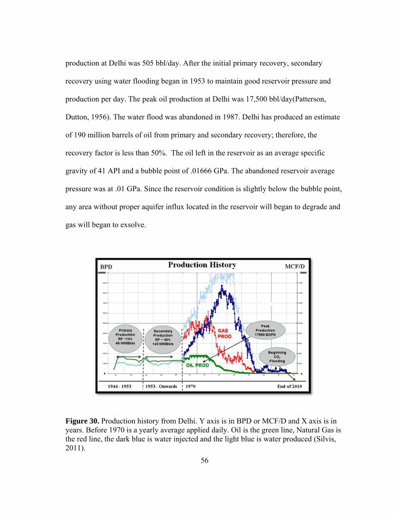
56

production at Delhi was 505 bbl/day. After the initial primary recovery, secondary

recovery using water flooding began in 1953 to maintain good reservoir pressure and

production per day. The peak oil production at Delhi was 17,500 bbl/day(Patterson,

Dutton, 1956). The water flood was abandoned in 1987. Delhi has produced an estimate

of 190 million barrels of oil from primary and secondary recovery; therefore, the

recovery factor is less than 50%. The oil left in the reservoir as an average specific

gravity of 41 API and a bubble point of .01666 GPa. The abandoned reservoir average

pressure was at .01 GPa. Since the reservoir condition is slightly below the bubble point,

any area without proper aquifer influx located in the reservoir will began to degrade and

gas will began to exsolve.

Figure 30. Production history from Delhi. Y axis is in BPD or MCF/D and X axis is in years. Before 1970 is a yearly average applied daily. Oil is the green line, Natural Gas is the red line, the dark blue is water injected and the light blue is water produced (Silvis, 2011).

57

On December 31, 2007, Denbury Resources spent $50 million on acquisition for

leases at the Delhi prospect. The Delhi reservoir was considered a supreme candidate for

CO2 flooding. These reasons include but are not limited to:

• CO2 should be effectively stored within the reservoir because it is

structurally simple with an unconformity forming a secure trap.

• The reservoir sands have high permeability and a water flood had already

been proven effective.

• The Delhi field is close to the Jackson Dome CO2 production facility

owned by Denbury and a pipeline for injection would be relatively

inexpensive.

In 2009 Denbury connected a pipeline from their CO2 reservoir located in

Jackson Mississippi and started injecting CO2 into Delhi. Denbury estimated probable

CO2 EOR reserves at Delhi to be 33 million barrels net to Denbury’s interest in the

reservoir (Evolution Petroleum Corporation, 2008). Denbury began CO2 EOR in

November of 2009 when nine injection wells began flooding the Tuscaloosa and Paluxy

sandstone reservoirs with CO2. Injection rates have varied per injector and day but on

average the injection rate for these 9 wells are 10 thousand cubic feet per day (Figure

31). The CO2 injection was into a reservoir with a pressure of approximately .01 giga

pascals (GPa). The injection increased the reservoir to approximately .013 GPa before

any production. Currently the reservoir pressure is at .015 GPa and is increasing due to

the amount of CO2 being injected into the reservoir.

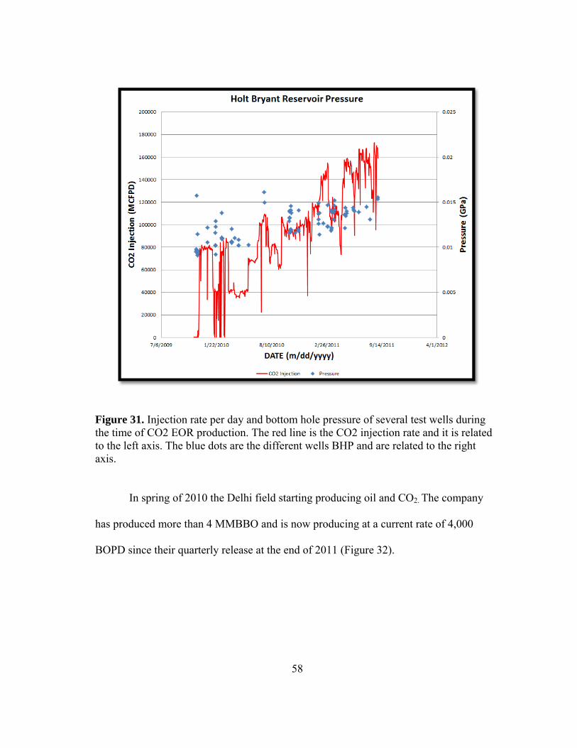
58

Figure 31. Injection rate per day and bottom hole pressure of several test wells during the time of CO2 EOR production. The red line is the CO2 injection rate and it is related to the left axis. The blue dots are the different wells BHP and are related to the right axis.

In spring of 2010 the Delhi field starting producing oil and CO2. The company

has produced more than 4 MMBBO and is now producing at a current rate of 4,000

BOPD since their quarterly release at the end of 2011 (Figure 32).

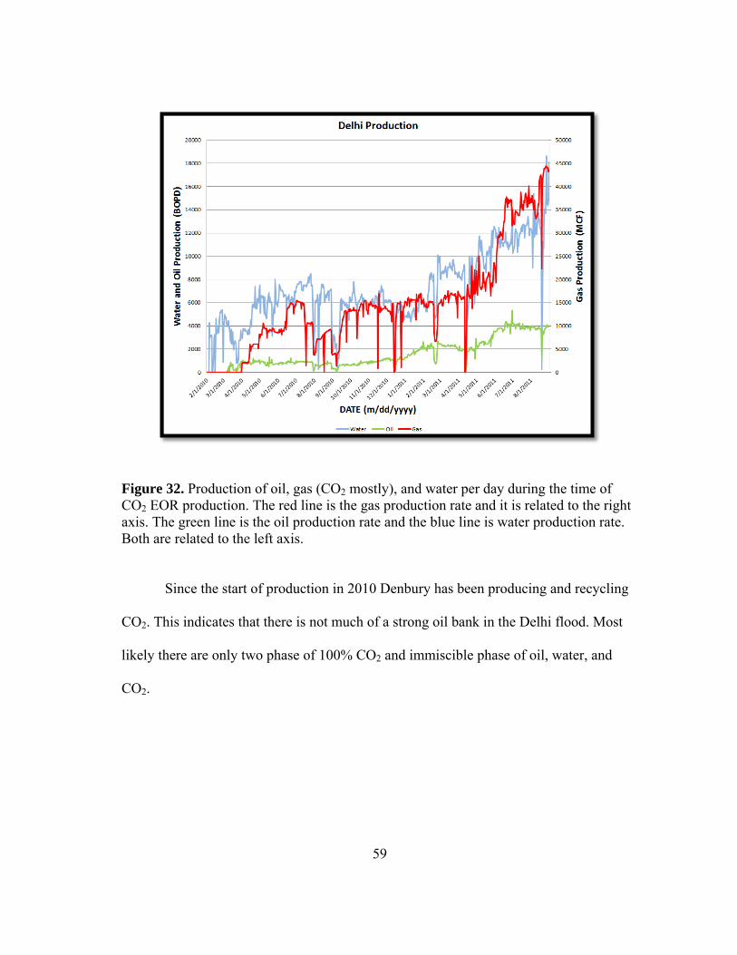
59

Figure 32. Production of oil, gas (CO2 mostly), and water per day during the time of CO2 EOR production. The red line is the gas production rate and it is related to the right axis. The green line is the oil production rate and the blue line is water production rate. Both are related to the left axis.

Since the start of production in 2010 Denbury has been producing and recycling

CO2. This indicates that there is not much of a strong oil bank in the Delhi flood. Most

likely there are only two phase of 100% CO2 and immiscible phase of oil, water, and

CO2.

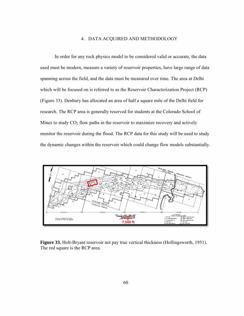
60

4. DATA ACQUIRED AND METHODOLOGY

In order for any rock physics model to be considered valid or accurate, the data

used must be modern, measure a variety of reservoir properties, have large range of data

spanning across the field, and the data must be measured over time. The area at Delhi

which will be focused on is referred to as the Reservoir Characterization Project (RCP)

(Figure 33). Denbury has allocated an area of half a square mile of the Delhi field for

research. The RCP area is generally reserved for students at the Colorado School of

Mines to study CO2 flow paths in the reservoir to maximize recovery and actively

monitor the reservoir during the flood. The RCP data for this study will be used to study

the dynamic changes within the reservoir which could change flow models substantially.

Figure 33. Holt-Bryant reservoir net pay true vertical thickness (Hollingsworth, 1951). The red square is the RCP area.

61

4.1 Data Acquired

In 2008, Denbury announced an $80 million budget for the Delhi Field

prospect(Denbury 2011). Most wells in Delhi were drilled prior to 1970. Prior to CO2

injection in 2009, Denbury was able to restore a majority of these wells and run current

well logs. In the RCP area there are 77 of these wells. After CO2 injection in 2010,

Denbury restored or drilled new wells to help production. A majority of these wells also

had current well logs run in the boreholes. In the RCP area there are 16 of these wells.

Some wells include: spontaneous potential, gamma ray, induction, nuclear magnetic

resonance, neutron porosity, bulk density, photoelectric, compressional and shear wave

sonic. Three wells contain all of these logs. One well was drilled post CO2 injection

(169-5), one well also has a core sample (159-2), and one well is an active injector (140-

1) in the Tuscaloosa and Paluxy reservoir. The lithology in the core sampled at well 159-

2 has been estimated using X-ray microscopy (XRM), Fourier Transform Infrared

Spectroscopy (FTIR) analysis and studying several thin sections in varying sections of

the Tuscaloosa and Paluxy. Denbury acquired 3D seismic before flooding in January

2009, a survey during injection in May 2010 and finally another survey done in Oct.

2011 (Figure 34 & 35).

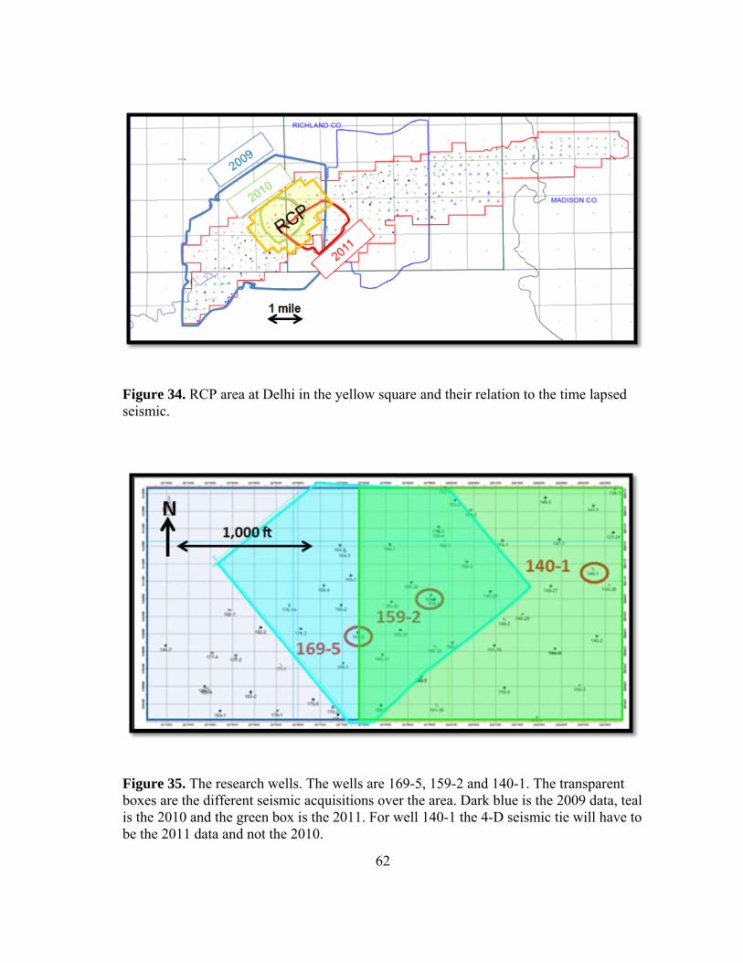
62

Figure 34. RCP area at Delhi in the yellow square and their relation to the time lapsed seismic.

Figure 35. The research wells. The wells are 169-5, 159-2 and 140-1. The transparent boxes are the different seismic acquisitions over the area. Dark blue is the 2009 data, teal is the 2010 and the green box is the 2011. For well 140-1 the 4-D seismic tie will have to be the 2011 data and not the 2010.

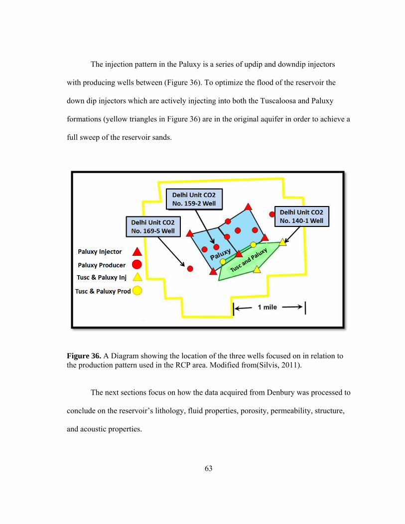
63

The injection pattern in the Paluxy is a series of updip and downdip injectors

with producing wells between (Figure 36). To optimize the flood of the reservoir the

down dip injectors which are actively injecting into both the Tuscaloosa and Paluxy

formations (yellow triangles in Figure 36) are in the original aquifer in order to achieve a

full sweep of the reservoir sands.

Figure 36. A Diagram showing the location of the three wells focused on in relation to the production pattern used in the RCP area. Modified from(Silvis, 2011).

The next sections focus on how the data acquired from Denbury was processed to

conclude on the reservoir’s lithology, fluid properties, porosity, permeability, structure,

and acoustic properties.

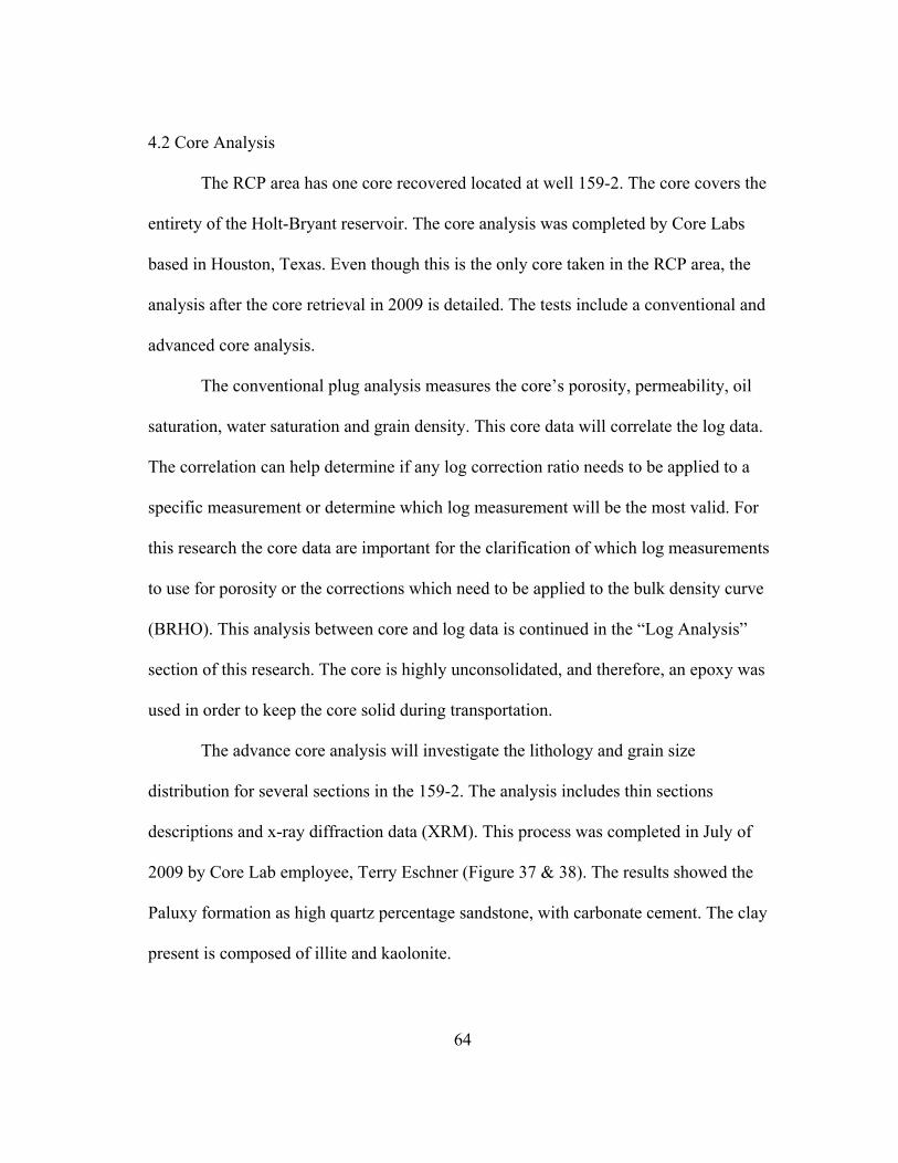
64

4.2 Core Analysis

The RCP area has one core recovered located at well 159-2. The core covers the

entirety of the Holt-Bryant reservoir. The core analysis was completed by Core Labs

based in Houston, Texas. Even though this is the only core taken in the RCP area, the

analysis after the core retrieval in 2009 is detailed. The tests include a conventional and

advanced core analysis.

The conventional plug analysis measures the core’s porosity, permeability, oil

saturation, water saturation and grain density. This core data will correlate the log data.

The correlation can help determine if any log correction ratio needs to be applied to a

specific measurement or determine which log measurement will be the most valid. For

this research the core data are important for the clarification of which log measurements

to use for porosity or the corrections which need to be applied to the bulk density curve

(BRHO). This analysis between core and log data is continued in the “Log Analysis”

section of this research. The core is highly unconsolidated, and therefore, an epoxy was

used in order to keep the core solid during transportation.

The advance core analysis will investigate the lithology and grain size

distribution for several sections in the 159-2. The analysis includes thin sections

descriptions and x-ray diffraction data (XRM). This process was completed in July of

2009 by Core Lab employee, Terry Eschner (Figure 37 & 38). The results showed the

Paluxy formation as high quartz percentage sandstone, with carbonate cement. The clay

present is composed of illite and kaolonite.

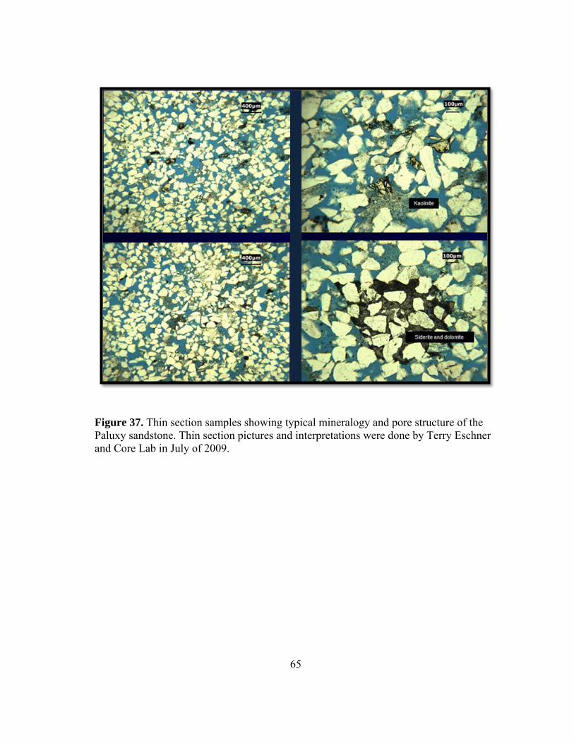
65

Figure 37. Thin section samples showing typical mineralogy and pore structure of the Paluxy sandstone. Thin section pictures and interpretations were done by Terry Eschner and Core Lab in July of 2009.

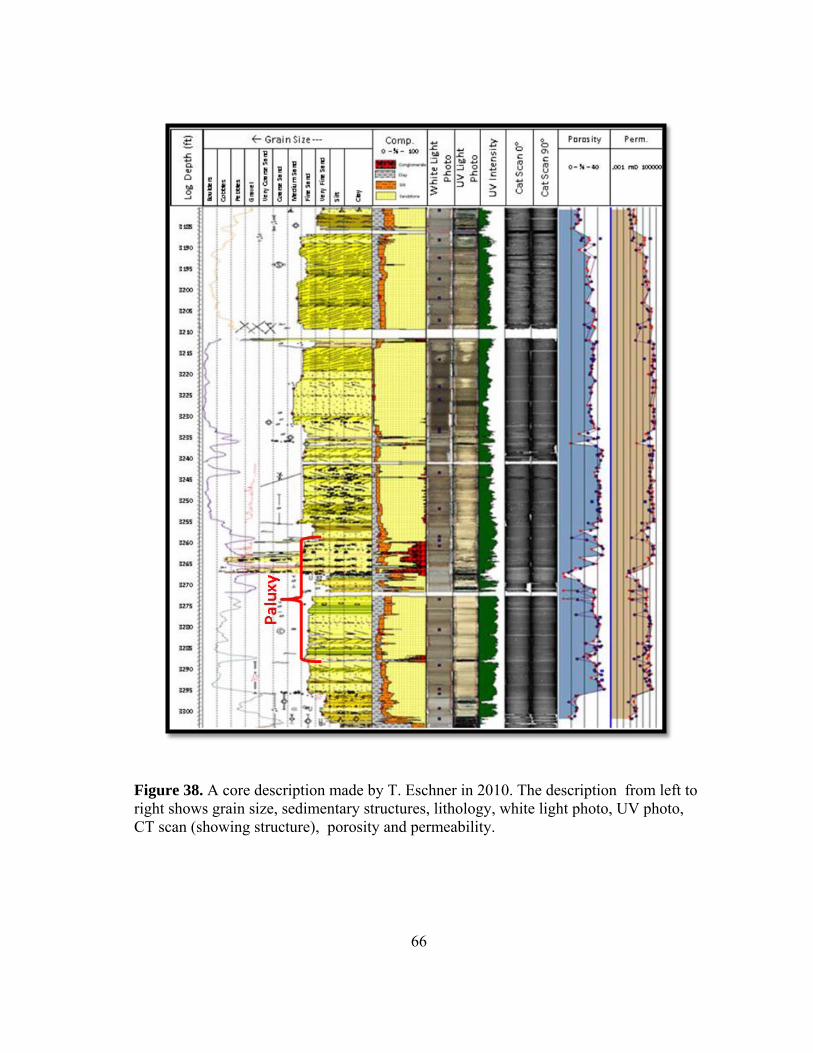
66

Figure 38. A core description made by T. Eschner in 2010. The description from left to right shows grain size, sedimentary structures, lithology, white light photo, UV photo, CT scan (showing structure), porosity and permeability.

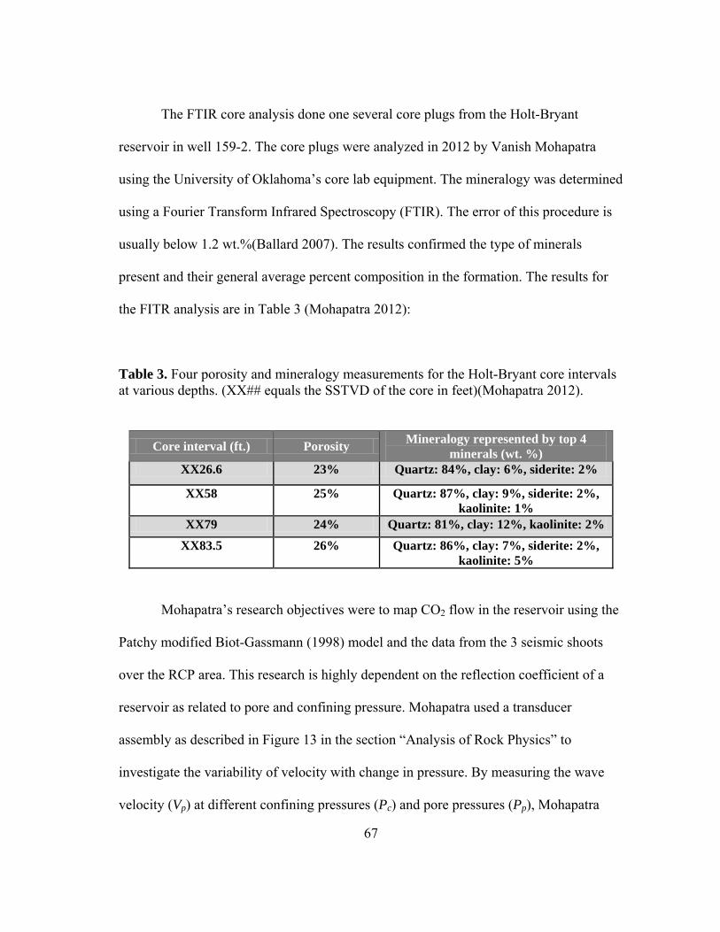
67

The FTIR core analysis done one several core plugs from the Holt-Bryant

reservoir in well 159-2. The core plugs were analyzed in 2012 by Vanish Mohapatra

using the University of Oklahoma’s core lab equipment. The mineralogy was determined

using a Fourier Transform Infrared Spectroscopy (FTIR). The error of this procedure is

usually below 1.2 wt.%(Ballard 2007). The results confirmed the type of minerals

present and their general average percent composition in the formation. The results for

the FITR analysis are in Table 3 (Mohapatra 2012):

Table 3. Four porosity and mineralogy measurements for the Holt-Bryant core intervals at various depths. (XX## equals the SSTVD of the core in feet)(Mohapatra 2012).

Core interval (ft.) Porosity Mineralogy represented by top 4 minerals (wt. %)

XX26.6 23% Quartz: 84%, clay: 6%, siderite: 2%

XX58 25% Quartz: 87%, clay: 9%, siderite: 2%, kaolinite: 1%

XX79 24% Quartz: 81%, clay: 12%, kaolinite: 2% XX83.5 26% Quartz: 86%, clay: 7%, siderite: 2%,

kaolinite: 5%

Mohapatra’s research objectives were to map CO2 flow in the reservoir using the

Patchy modified Biot-Gassmann (1998) model and the data from the 3 seismic shoots

over the RCP area. This research is highly dependent on the reflection coefficient of a

reservoir as related to pore and confining pressure. Mohapatra used a transducer

assembly as described in Figure 13 in the section “Analysis of Rock Physics” to

investigate the variability of velocity with change in pressure. By measuring the wave

velocity (Vp) at different confining pressures (Pc) and pore pressures (Pp), Mohapatra

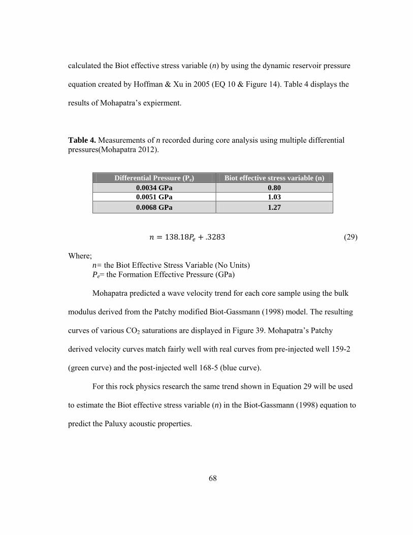
68

calculated the Biot effective stress variable (n) by using the dynamic reservoir pressure

equation created by Hoffman & Xu in 2005 (EQ 10 & Figure 14). Table 4 displays the

results of Mohapatra’s expierment.

Table 4. Measurements of n recorded during core analysis using multiple differential pressures(Mohapatra 2012).

Differential Pressure (Pe) Biot effective stress variable (n) 0.0034 GPa 0.80 0.0051 GPa 1.03 0.0068 GPa 1.27

𝑛 = 138.18𝑃𝑒 + .3283 (29)

Where; n= the Biot Effective Stress Variable (No Units) Pe= the Formation Effective Pressure (GPa)

Mohapatra predicted a wave velocity trend for each core sample using the bulk

modulus derived from the Patchy modified Biot-Gassmann (1998) model. The resulting

curves of various CO2 saturations are displayed in Figure 39. Mohapatra’s Patchy

derived velocity curves match fairly well with real curves from pre-injected well 159-2

(green curve) and the post-injected well 168-5 (blue curve).

For this rock physics research the same trend shown in Equation 29 will be used

to estimate the Biot effective stress variable (n) in the Biot-Gassmann (1998) equation to

predict the Paluxy acoustic properties.

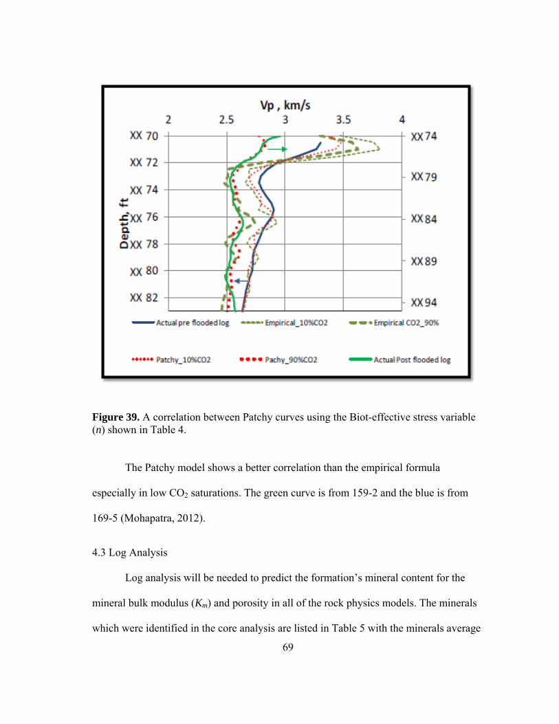
69

Figure 39. A correlation between Patchy curves using the Biot-effective stress variable (n) shown in Table 4.

The Patchy model shows a better correlation than the empirical formula

especially in low CO2 saturations. The green curve is from 159-2 and the blue is from

169-5 (Mohapatra, 2012).

4.3 Log Analysis

Log analysis will be needed to predict the formation’s mineral content for the

mineral bulk modulus (Km) and porosity in all of the rock physics models. The minerals

which were identified in the core analysis are listed in Table 5 with the minerals average

70

log characteristics. The sonic properties of the mineral were not used during log analysis.

This is to avoid consistency bias errors since the mineral interpretation from the log will

be used to measure the mineral bulk modulus.

The logs used to calculate water saturation (Sw) are the induction and nuclear

magnetic resonance imaging (MRI) log. Archie’s equation uses the resistivity measured

from the induction log and the formation water salinity to estimate water saturation.

𝑅𝑡 = 𝑎𝜙−𝑚𝑆𝑤−𝑛𝑅𝑤 (30)

Where; Rt= Measured Resistivity (ohm.m) m=1 Rw= Resistivity of Formation Water (ohm.m) n=2 ϕ= Porosity (%) a=1 Sw= Water Saturation (%)

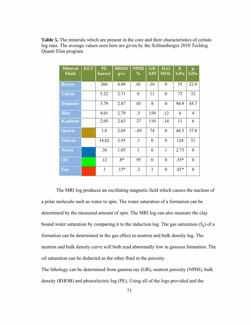
71

Table 5. The minerals which are present in the core and their characteristics of certain log runs. The average values seen here are given by the Schlumberger 2010 Techlog Quanti Elan program.

Mineral Fluid

KEY PE barn/e

BRHO g/cc

NPHI %

GR API

H2O MOL

K GPa

µ GPa

Baryte 266 4.08 .01 .01 0 55 22.8

Calcite 5.22 2.71 0 11 0 73 32

Dolomite 3.79 2.87 .03 8 0 94.9 45.7

Illite 4.01 2.79 .3 150 .12 6 4

Kaolinite 2.05 2.63 .37 110 .14 11 6

Quartz 1.8 2.65 -.03 74 0 44.3 37.8

Siderite 14.62 3.93 .1 0 0 124 51

Water .36 1.05 1 0 1 2.73 0

Oil .12 .8* .95 0 0 .55* 0

Gas .1 .15* .2 1 0 .01* 0

The MRI log produces an oscillating magnetic field which causes the nucleus of

a polar molecule such as water to spin. The water saturation of a formation can be

determined by the measured amount of spin. The MRI log can also measure the clay

bound water saturation by comparing it to the induction log. The gas saturation (Sg) of a

formation can be determined in the gas effect in neutron and bulk density log. The

neutron and bulk density curve will both read abnormally low in gaseous formation. The

oil saturation can be deducted as the other fluid in the porosity.

The lithology can be determined from gamma ray (GR), neutron porosity (NPHI), bulk

density (RHOB) and photoelectric log (PE). Using all of the logs provided and the

72

average log properties of each mineral an estimation of lithology can be made. The

estimation is done by using an algorithm in Schlumberger 2010 Techlog Quanti Elan

program. Quanti Elan uses a process called sequential quadratic programming (SQP).

The SQP is an iterative method similar the cluster or grouping method, but SQP can be

applied to more dimensions than three. Each log parameter listed will be used as a

variable to best calculate the lithology of the formation, except the sonic logs and the

bulk and shear modulus in the table are not used for consistency bias errors. The results

compared to the core data ensure the accuracy of the Tech Log calculations. The trends

between the two data sets are satisfactory (Figure 40). The derived Quanti Elan well logs

will be used for all rock physics modeling during this research where every log listed in

the table is present. The results are seen in Figure 41.

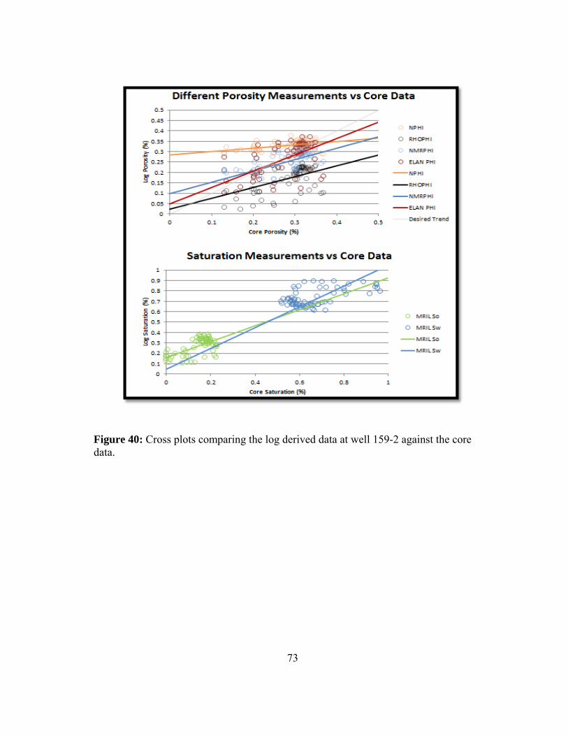
73

Figure 40: Cross plots comparing the log derived data at well 159-2 against the core data.

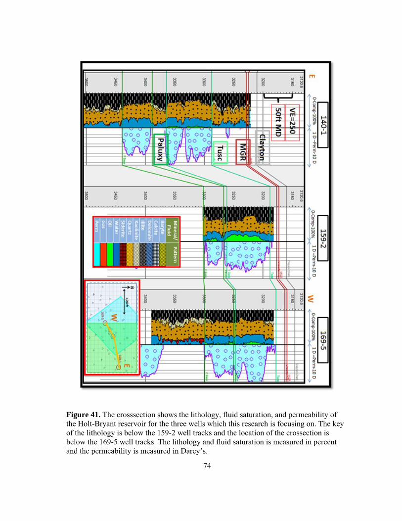
74

Figure 41. The crosssection shows the lithology, fluid saturation, and permeability of the Holt-Bryant reservoir for the three wells which this research is focusing on. The key of the lithology is below the 159-2 well tracks and the location of the crossection is below the 169-5 well tracks. The lithology and fluid saturation is measured in percent and the permeability is measured in Darcy’s.

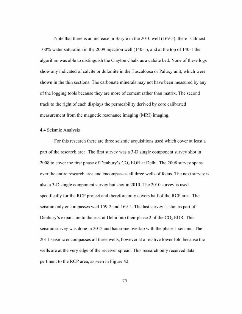
75

Note that there is an increase in Baryte in the 2010 well (169-5), there is almost

100% water saturation in the 2009 injection well (140-1), and at the top of 140-1 the

algorithm was able to distinguish the Clayton Chalk as a calcite bed. None of these logs

show any indicated of calcite or dolomite in the Tuscaloosa or Paluxy unit, which were

shown in the thin sections. The carbonate minerals may not have been measured by any

of the logging tools because they are more of cement rather than matrix. The second

track to the right of each displays the permeability derived by core calibrated

measurement from the magnetic resonance imaging (MRI) imaging.

4.4 Seismic Analysis

For this research there are three seismic acquisitions used which cover at least a

part of the research area. The first survey was a 3-D single component survey shot in

2008 to cover the first phase of Denbury’s CO2 EOR at Delhi. The 2008 survey spans

over the entire research area and encompasses all three wells of focus. The next survey is

also a 3-D single component survey but shot in 2010. The 2010 survey is used

specifically for the RCP project and therefore only covers half of the RCP area. The

seismic only encompasses well 159-2 and 169-5. The last survey is shot as part of

Denbury’s expansion to the east at Delhi into their phase 2 of the CO2 EOR. This

seismic survey was done in 2012 and has some overlap with the phase 1 seismic. The

2011 seismic encompasses all three wells, however at a relative lower fold because the

wells are at the very edge of the receiver spread. This research only received data

pertinent to the RCP area, as seen in Figure 42.

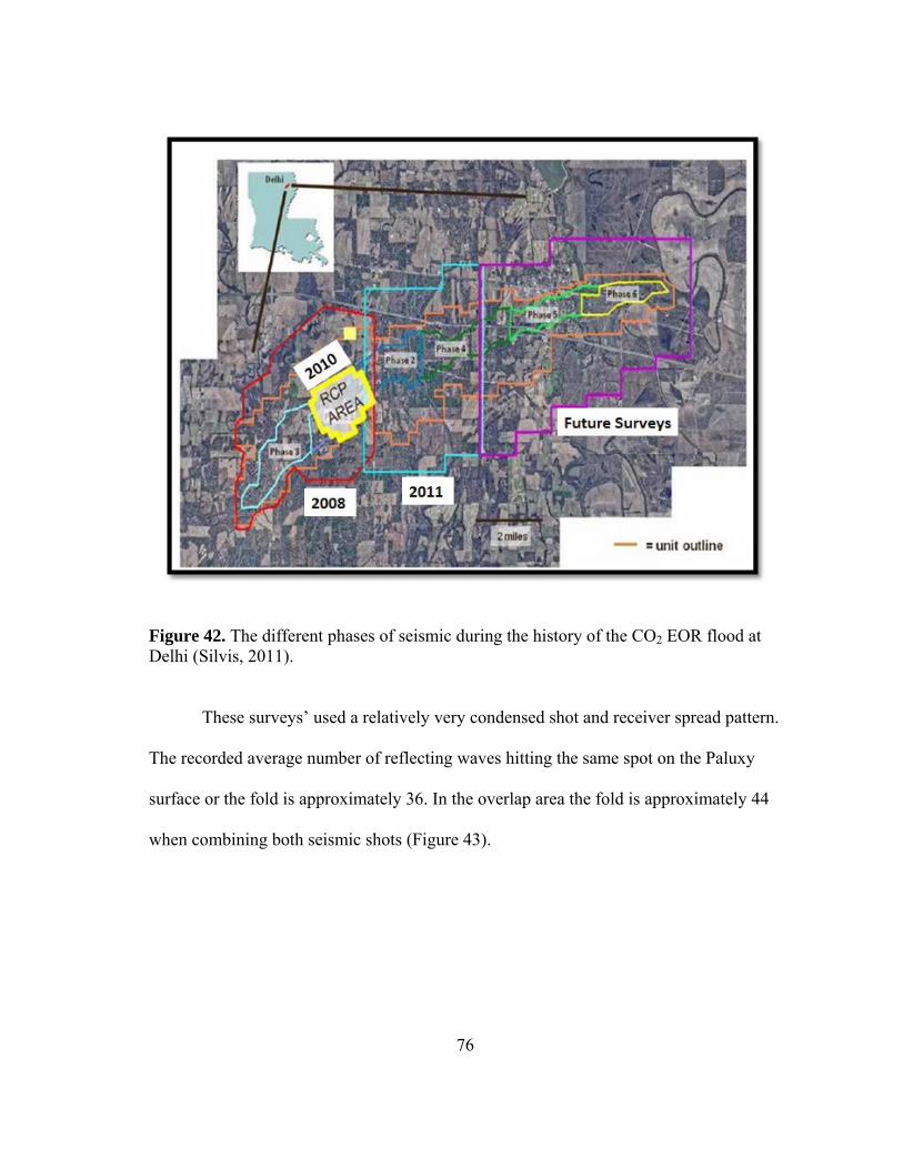
76

Figure 42. The different phases of seismic during the history of the CO2 EOR flood at Delhi (Silvis, 2011).

These surveys’ used a relatively very condensed shot and receiver spread pattern.

The recorded average number of reflecting waves hitting the same spot on the Paluxy

surface or the fold is approximately 36. In the overlap area the fold is approximately 44

when combining both seismic shots (Figure 43).

77

Figure 43. The seismic fold over the Delhi region. The RCP area is in black. The scale for fold is on the right. The increase in fold is due to overlap.

This allows very detailed and accurate seismic attribute mapping to be done on

the individual sand units. For the purpose of this research only the top of the Paluxy,

Tuscaloosa unit, and Clayton Chalk were mapped for each seismic survey.

Seismic mapping requires a synthetic seismogram created from wells which

contains a density and sonic log. These logs will be used to create a reflection coefficient

log (EQ 1 & Figure 11) which will be multiplied by a wavelet. The best wavelet to use

for a well tie in the RCP area is a 60 Hz Ricker wave with a 0 phase offset and a wave

length of 120 ms. For the 2009 seismic shoot there were 6 wells which contained these

logs, including 159-2 and 140-1 (Figure 44). The synthetic correlated the Paluxy surface

to a weak peak amplitude signal in the reservoir area, such as in 159-2. However the

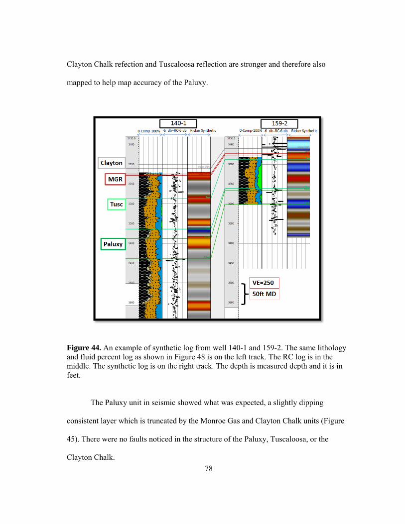
78

Clayton Chalk refection and Tuscaloosa reflection are stronger and therefore also

mapped to help map accuracy of the Paluxy.

Figure 44. An example of synthetic log from well 140-1 and 159-2. The same lithology and fluid percent log as shown in Figure 48 is on the left track. The RC log is in the middle. The synthetic log is on the right track. The depth is measured depth and it is in feet.

The Paluxy unit in seismic showed what was expected, a slightly dipping

consistent layer which is truncated by the Monroe Gas and Clayton Chalk units (Figure

45). There were no faults noticed in the structure of the Paluxy, Tuscaloosa, or the

Clayton Chalk.

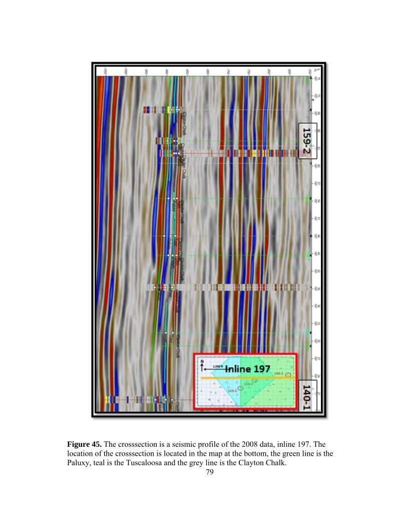
79

Figure 45. The crosssection is a seismic profile of the 2008 data, inline 197. The location of the crosssection is located in the map at the bottom, the green line is the Paluxy, teal is the Tuscaloosa and the grey line is the Clayton Chalk.

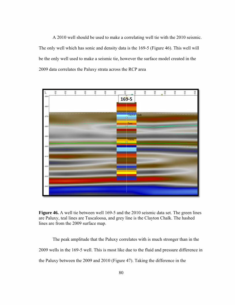
80

A 2010 well should be used to make a correlating well tie with the 2010 seismic.

The only well which has sonic and density data is the 169-5 (Figure 46). This well will

be the only well used to make a seismic tie, however the surface model created in the

2009 data correlates the Paluxy strata across the RCP area

Figure 46. A well tie between well 169-5 and the 2010 seismic data set. The green lines are Paluxy, teal lines are Tuscaloosa, and grey line is the Clayton Chalk. The hashed lines are from the 2009 surface map.

The peak amplitude that the Paluxy correlates with is much stronger than in the

2009 wells in the 169-5 well. This is most like due to the fluid and pressure difference in

the Paluxy between the 2009 and 2010 (Figure 47). Taking the difference in the

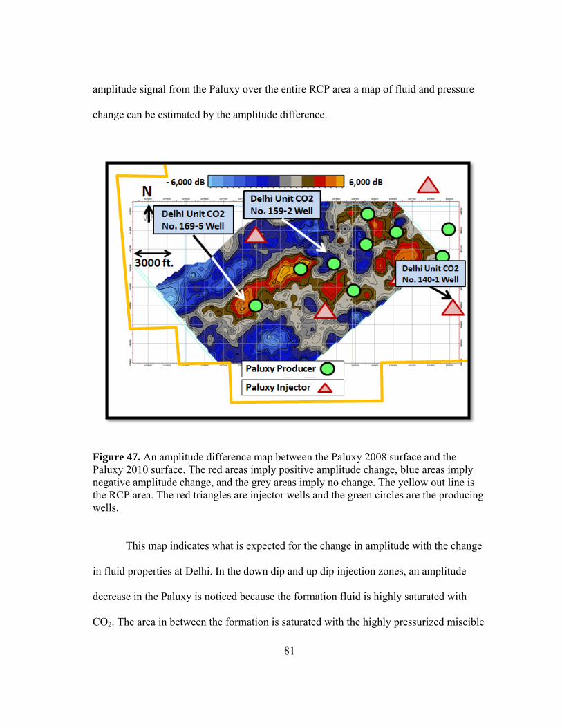
81

amplitude signal from the Paluxy over the entire RCP area a map of fluid and pressure

change can be estimated by the amplitude difference.

Figure 47. An amplitude difference map between the Paluxy 2008 surface and the Paluxy 2010 surface. The red areas imply positive amplitude change, blue areas imply negative amplitude change, and the grey areas imply no change. The yellow out line is the RCP area. The red triangles are injector wells and the green circles are the producing wells.

This map indicates what is expected for the change in amplitude with the change

in fluid properties at Delhi. In the down dip and up dip injection zones, an amplitude

decrease in the Paluxy is noticed because the formation fluid is highly saturated with

CO2. The area in between the formation is saturated with the highly pressurized miscible

82

phase of oil, water and CO2. This would create the amplitude increase we see in the

production zone and in the producing well 169-5.

The 2011 data set will be used to create a well tie with a fluid substitute model of

well 140-1. This well tie will show any rock physics changes noticed because of CO2

interaction with the formation

4.5 Methodology

To compare the formation’s rock properties, two time-lapsed wells will be

needed for analysis. The wells will need sufficient amount of logs to predict saturation,

lithology and bulk and shear modulus. The wells will also need to be in a similar

original depositional facie. The Paluxy reservoir is deposited in a Delta plain. This

environment deposits homogenous and isotropic formations which are usually laterally

continuous in rock properties. Still, two wells relatively close to each other would

provide better data. The 2009 well 159-2 and 2010 well 169-5 are prime candidates for

this research. They are separated by 1,567 feet, and both wells have ample amount of log

data for all petro-physical and sonic analysis.

To perform a fluid substitution a well will need a simple fluid exchange to

minimize errors since Gassmann (1998) equation will be used to derive the dry bulk

modulus (Kd). The CO2 flood at the Delhi Field is an immiscible flood because the

reservoir pressure is lower than the minimum miscibility pressure (MMP)(Silvis 2011).

An immiscible flood does not create a homogeneous fluid in the reservoir. Instead, an

immiscible flood will create a CO2 phase next to the injection well, then fading to a

83

miscible zone and finally an oil bank. The CO2 saturation near the injection wells post-

injection to be at nearly 100%.

Well 140-1 is an injector and is in the original Paluxy aquifer prior to CO2

injection. This makes the 2009 well 140-1 a supreme well for a fluid substitution

because the water saturation is 100% pre-injection and the CO2 saturation is 100%. More

importantly the CO2 physical state is known. The CO2 phase is essential in measuring

rock physic properties because CO2 injected is at a supercritical state due to the pressure

and temperature of the reservoir causing additional amplitude increase of about 7% than

liquid CO2 due to increase pore pressure(Yuh 2004).

Using the wells 140-1, 159-2, and 169-5 the objective of determining rock physic

changes can be accomplished using the following steps:

1. Find a best model for the all three wells using the rock physics theories in section

2.

2. Calculate the dry bulk modulus using the best fit model and the Gassmann (1998)

equation.

3. Determine if there is any difference in lithology, porosity, permeability between

a well drilled post CO2 flood in 2010 (160-5) and pre CO2 flood in 2009 (159-2)

in the Paluxy reservoir. These two wells are Ideal candidates for comparison

because they are only 1567m apart in a similar facie sand deposit.

4. Determine if the two wells in the Paluxy have different acoustic data which can

be associated with the change of the lithology, porosity, or permeability.

84

5. Create a synthetic seismogram from a fluid substitution, making no changes to

the dry bulk modulus or pore structure (ˠ) using the injection well 140-1. Well

140-1 will be used for fluid substitution because the saturation values can be

predicted without using a model (Patchy) to derive saturation. The well is drilled

in the original Paluxy aquifer (≈100% water pre-flood) and is an injection well

(≈100% CO2 post-flood).

6. Create a synthetic seismogram from a fluid substitution for 140-1, but change the

dry bulk modulus with respect to the change in the framework work flexibility

factor (γ) (EQ 25) observed between 160-5 and 159-2.

7. Make a well tie to for both to the actual seismic in shot in 2011 and compare and

contrast.

85

5. RESULTS

This section presents the evidence of rock property changes between pre- and

post-CO2 flood by focusing on the application of the rock physics models. The two wells

159-2 and 169-1 are compared based solely on log and core data to observe changes. To

show correlation between the log and acoustic data the rock-physic models presented in

section two “Analysis of Reservoir rock Physics” was used to model the velocity from

non-sonic log data. The Raymer (1980) equation has the best fit to the actual sonic data.

The measurements from sonic for the pre-CO2 flood wells (140-1 and 159-2) and the

post-CO2 flood wells (169-5) was plotted against Tech Log calculated porosity to

understand the pore influence on the formation velocity. The pore space bulk modulus

was calculated and plotted against porosity and the Baechle (2005) ratio trend lines to

reveal the changes in micro or macro porosity. The frame work flexibility factor is

plotted against porosity to determine the grain boundary behavior in the formation. To

further prove the pore structure changes in the Paluxy a fluid substitution calculation on

140-1 in a 100% CO2 scenario was calculated. The calculations include two synthetic

seismograms. The first model used the original frame work flexibility and dry bulk

modulus. The second model will use a diagenetic change in both moduli as observed in

the difference between 159-2 and 169-5. The synthetic seismograms are calculated by

the velocity estimation from Raymer (1980) and Gassmann’s (1998) equation. The

synthetic seismograms are compared to the 2011 seismic acquisition to observe which

has the best tie.

86

5.1 Wells 159-2 and 169-5 Variability in Lithology, Porosity and Permeability

Well 159-2 and 169-5 are separated by approximately 18,500 feet. Since the

Paluxy is determined to be deposited in a delta plain, the Paluxy original rock physics

properties in both wells are assumed to be fairly similar. Well 159-2 was drilled before

the CO2 flood in 2009 and well 169-5 was drilled post CO2 flood in 2010. First both

wells lithology and permeability log measurements will be compared in order to see any

difference which is not associated with the acoustic properties of the formation.

The comparison in lithology reveals that the only change between the 2009 and

2010 wells is a slight increase in barite observed in the 2010 169-5 well (Figure 48).

Both wells increase in kaolinite and siderite with a decrease in porosity and have an

approximately 60% quartz and 40% illite across the porosity range in the Paluxy

reservoir. The reservoir also likely has some carbonate cement as observed in thin

section and core analysis.

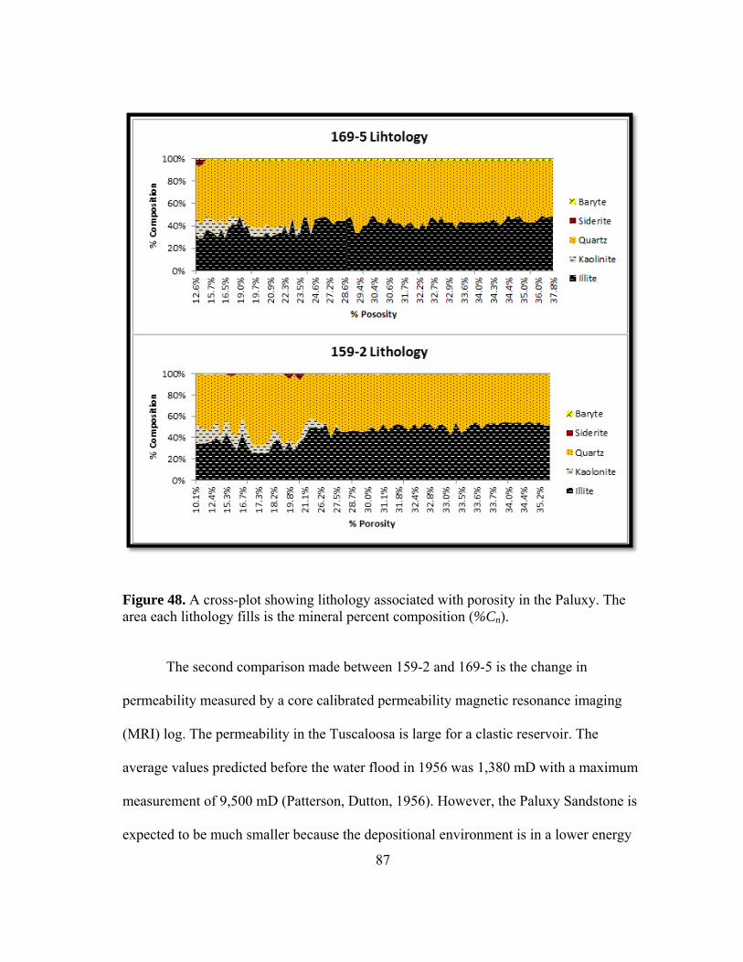
87

Figure 48. A cross-plot showing lithology associated with porosity in the Paluxy. The area each lithology fills is the mineral percent composition (%Cn).

The second comparison made between 159-2 and 169-5 is the change in

permeability measured by a core calibrated permeability magnetic resonance imaging

(MRI) log. The permeability in the Tuscaloosa is large for a clastic reservoir. The

average values predicted before the water flood in 1956 was 1,380 mD with a maximum

measurement of 9,500 mD (Patterson, Dutton, 1956). However, the Paluxy Sandstone is

expected to be much smaller because the depositional environment is in a lower energy

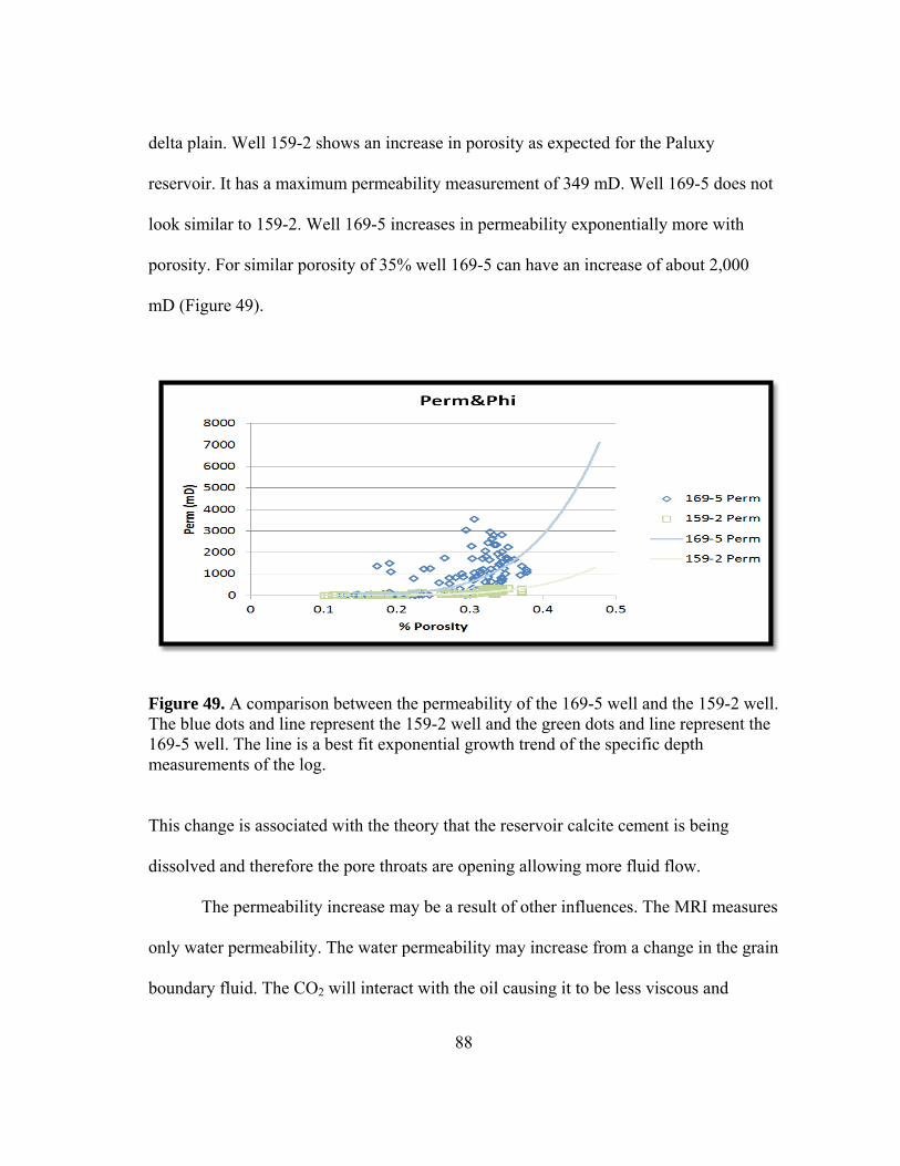
88

delta plain. Well 159-2 shows an increase in porosity as expected for the Paluxy

reservoir. It has a maximum permeability measurement of 349 mD. Well 169-5 does not

look similar to 159-2. Well 169-5 increases in permeability exponentially more with

porosity. For similar porosity of 35% well 169-5 can have an increase of about 2,000

mD (Figure 49).

Figure 49. A comparison between the permeability of the 169-5 well and the 159-2 well. The blue dots and line represent the 159-2 well and the green dots and line represent the 169-5 well. The line is a best fit exponential growth trend of the specific depth measurements of the log.

This change is associated with the theory that the reservoir calcite cement is being

dissolved and therefore the pore throats are opening allowing more fluid flow.

The permeability increase may be a result of other influences. The MRI measures

only water permeability. The water permeability may increase from a change in the grain

boundary fluid. The CO2 will interact with the oil causing it to be less viscous and

89

release from grains. Another reason is that even though the deposition likely is laterally

continuous, there is evidence of some channel flows. This may also be the reason for the

permeability change.

5.2 Velocity Estimation Rock Physic Models

The rock physic models to correlate logs to sonic data are the Voigt, Reuss, Hill

Average, Wyllie (1958), and Raymer (1980). Each model will use the saturation and

mineral logs and the average values of each composition’s modulus (Table 5) to create

synthetic p-wave velocity curve. Each models velocity curve will be cross-plotted

against porosity with the original velocity derived from the sonic log. The Raymer

(1980) shows the best fit line between the three wells of 140-1, 159-2 and 169-5 and

used to predict the effective modulus for well 140-1 during fluid substitution.

The graphs display that the models from section 2 can be applied to predict the

bulk modulus very well in the Paluxy sandstone (Figure 50). The data points are

restricted to the Reuss or Voigt limit and all three trend lines show a close approximation

to the actual data. The trend line which fits the best is the Raymer (1980) model. In well

169-5 the Raymer (1980) is the only model which accurately predicts the velocity. This

model is what will be used to predict the dry bulk modulus in the Paluxy.

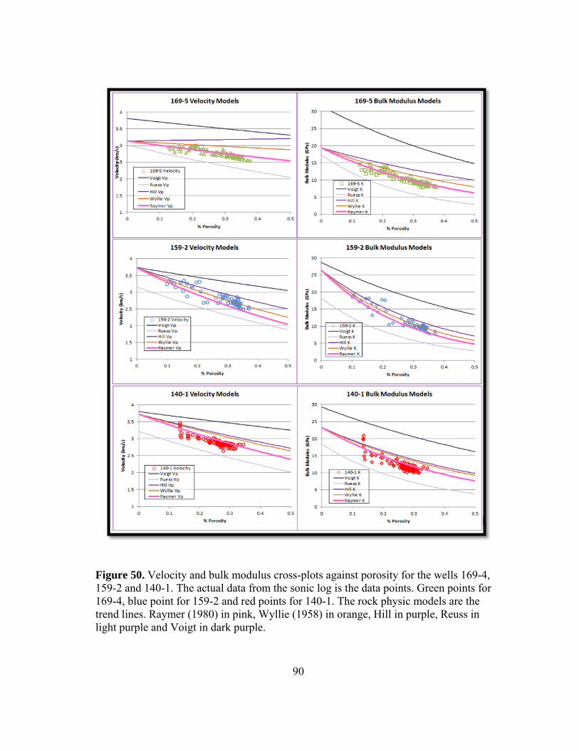
90

Figure 50. Velocity and bulk modulus cross-plots against porosity for the wells 169-4, 159-2 and 140-1. The actual data from the sonic log is the data points. Green points for 169-4, blue point for 159-2 and red points for 140-1. The rock physic models are the trend lines. Raymer (1980) in pink, Wyllie (1958) in orange, Hill in purple, Reuss in light purple and Voigt in dark purple.

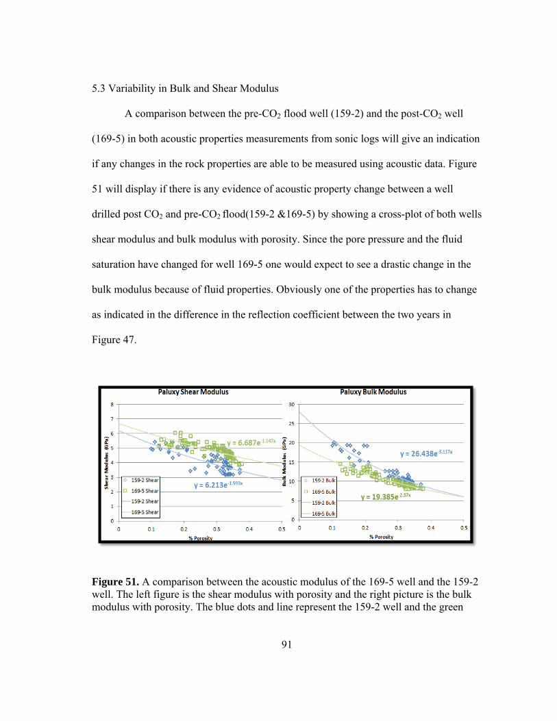
91

5.3 Variability in Bulk and Shear Modulus

A comparison between the pre-CO2 flood well (159-2) and the post-CO2 well

(169-5) in both acoustic properties measurements from sonic logs will give an indication

if any changes in the rock properties are able to be measured using acoustic data. Figure

51 will display if there is any evidence of acoustic property change between a well

drilled post CO2 and pre-CO2 flood(159-2 &169-5) by showing a cross-plot of both wells

shear modulus and bulk modulus with porosity. Since the pore pressure and the fluid

saturation have changed for well 169-5 one would expect to see a drastic change in the

bulk modulus because of fluid properties. Obviously one of the properties has to change

as indicated in the difference in the reflection coefficient between the two years in

Figure 47.

Figure 51. A comparison between the acoustic modulus of the 169-5 well and the 159-2 well. The left figure is the shear modulus with porosity and the right picture is the bulk modulus with porosity. The blue dots and line represent the 159-2 well and the green

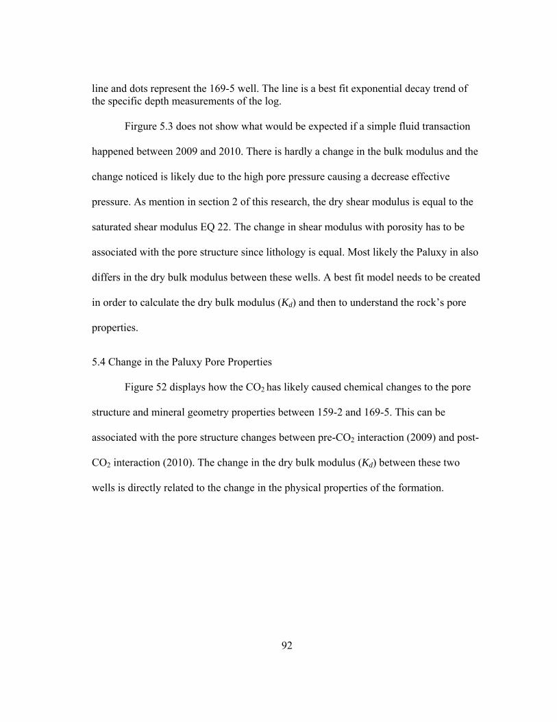
92

line and dots represent the 169-5 well. The line is a best fit exponential decay trend of the specific depth measurements of the log.

Firgure 5.3 does not show what would be expected if a simple fluid transaction

happened between 2009 and 2010. There is hardly a change in the bulk modulus and the

change noticed is likely due to the high pore pressure causing a decrease effective

pressure. As mention in section 2 of this research, the dry shear modulus is equal to the

saturated shear modulus EQ 22. The change in shear modulus with porosity has to be

associated with the pore structure since lithology is equal. Most likely the Paluxy in also

differs in the dry bulk modulus between these wells. A best fit model needs to be created

in order to calculate the dry bulk modulus (Kd) and then to understand the rock’s pore

properties.

5.4 Change in the Paluxy Pore Properties

Figure 52 displays how the CO2 has likely caused chemical changes to the pore

structure and mineral geometry properties between 159-2 and 169-5. This can be

associated with the pore structure changes between pre-CO2 interaction (2009) and post-

CO2 interaction (2010). The change in the dry bulk modulus (Kd) between these two

wells is directly related to the change in the physical properties of the formation.

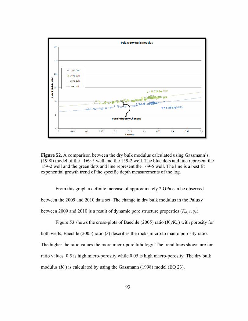
93

Figure 52. A comparison between the dry bulk modulus calculated using Gassmann’s (1998) model of the 169-5 well and the 159-2 well. The blue dots and line represent the 159-2 well and the green dots and line represent the 169-5 well. The line is a best fit exponential growth trend of the specific depth measurements of the log.

From this graph a definite increase of approximately 2 GPa can be observed

between the 2009 and 2010 data set. The change in dry bulk modulus in the Paluxy

between 2009 and 2010 is a result of dynamic pore structure properties (Kϕ, γ, γµ).

Figure 53 shows the cross-plots of Baechle (2005) ratio (Kd/Km) with porosity for

both wells. Baechle (2005) ratio (k) describes the rocks micro to macro porosity ratio.

The higher the ratio values the more micro-pore lithology. The trend lines shown are for

ratio values. 0.5 is high micro-porosity while 0.05 is high macro-porosity. The dry bulk

modulus (Kd) is calculated by using the Gassmann (1998) model (EQ 23).

94

Figure 53. A comparison between the Baechle (2005) ratio and porosity of the 169-5 well and the 159-2 well. The top graph is well 159-2 and the bottom graph is well 169-5. The symbols indicate type of porosity which is shown by thin sections to the left. Thin sections are from Terry Eschner 2009.

Since the lithology is observed as fairly consistent over the porosity in the Paluxy, the

prevailing factor for the Baechle (2005) ratio is the pore space bulk modulus (Kϕ) and

dry bulk modulus (Kd). The graph shows that the Paluxy in 169-5 on average has areas

with much higher pore space bulk moduli. This indicates that after the CO2 injection the

Paluxy formation has become more homogenous in pore structure.

Figure 54 is a cross plot of the effective bulk modulus (Ke) from the sonic logs

with porosity. The trend lines shown in the cross-plots are the same best fit exponential

decaying lines shown in Figure 50. To quantify a data point deviation from the best fit

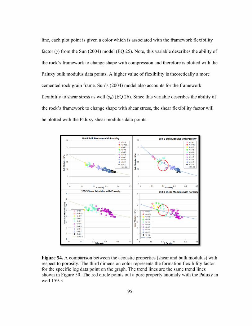
95

line, each plot point is given a color which is associated with the framework flexibility

factor (γ) from the Sun (2004) model (EQ 25). Note, this variable describes the ability of

the rock’s framework to change shape with compression and therefore is plotted with the

Paluxy bulk modulus data points. A higher value of flexibility is theoretically a more

cemented rock grain frame. Sun’s (2004) model also accounts for the framework

flexibility to shear stress as well (γµ) (EQ 26). Since this variable describes the ability of

the rock’s framework to change shape with shear stress, the shear flexibility factor will

be plotted with the Paluxy shear modulus data points.

well 159-3.

Figure 54. A comparison between the acoustic properties (shear and bulk modulus) with respect to porosity. The third dimension color represents the formation flexibility factor for the specific log data point on the graph. The trend lines are the same trend lines

shown in Figure 50. The red circle points out a pore property anomaly with the Paluxy in

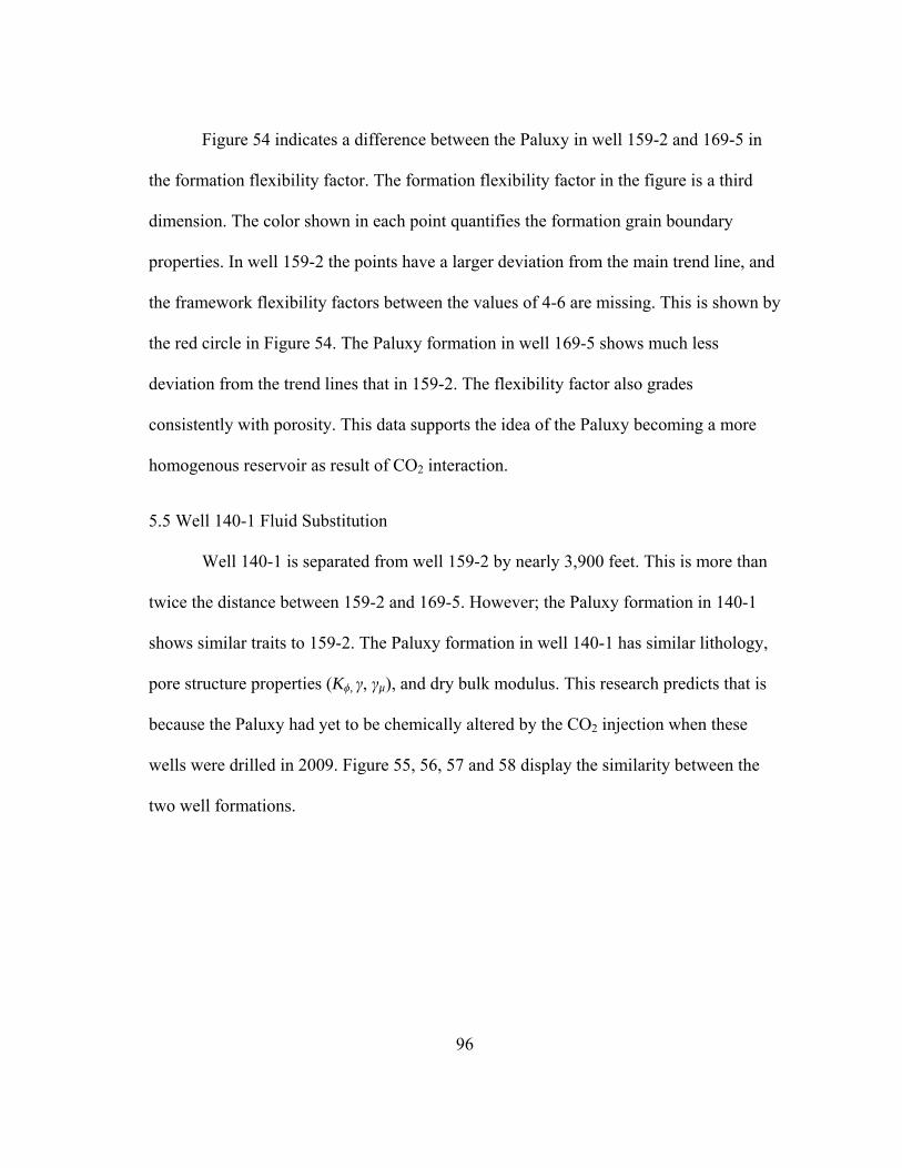
96

Figure 54 indicates a difference between the Paluxy in well 159-2 and 169-5 in

the formation flexibility factor. The formation flexibility factor in the figure is a third

dimension. The color shown in each point quantifies the formation grain boundary

properties. In well 159-2 the points have a larger deviation from the main trend line, and

the framework flexibility factors between the values of 4-6 are missing. This is shown by

the red circle in Figure 54. The Paluxy formation in well 169-5 shows much less

deviation from the trend lines that in 159-2. The flexibility factor also grades

consistently with porosity. This data supports the idea of the Paluxy becoming a more

homogenous reservoir as result of CO2 interaction.

5.5 Well 140-1 Fluid Substitution

Well 140-1 is separated from well 159-2 by nearly 3,900 feet. This is more than

twice the distance between 159-2 and 169-5. However; the Paluxy formation in 140-1

shows similar traits to 159-2. The Paluxy formation in well 140-1 has similar lithology,

pore structure properties (Kϕ, γ, γµ), and dry bulk modulus. This research predicts that is

because the Paluxy had yet to be chemically altered by the CO2 injection when these

wells were drilled in 2009. Figure 55, 56, 57 and 58 display the similarity between the

two well formations.

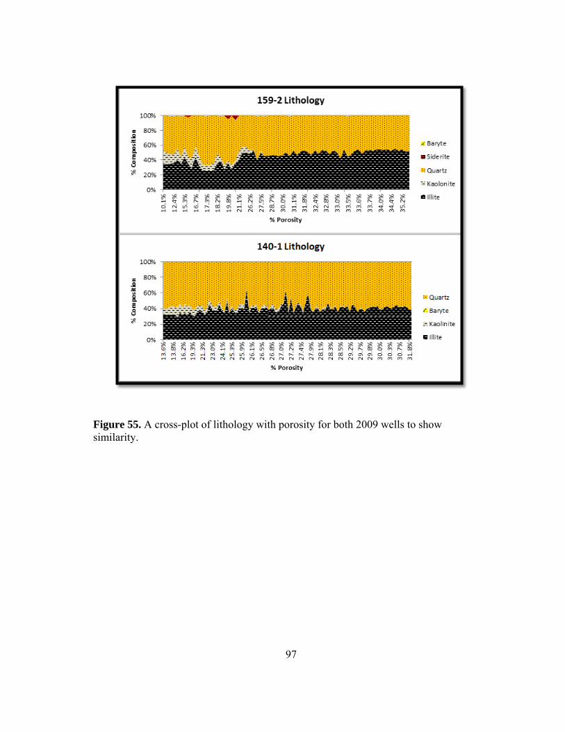
97

Figure 55. A cross-plot of lithology with porosity for both 2009 wells to show similarity.

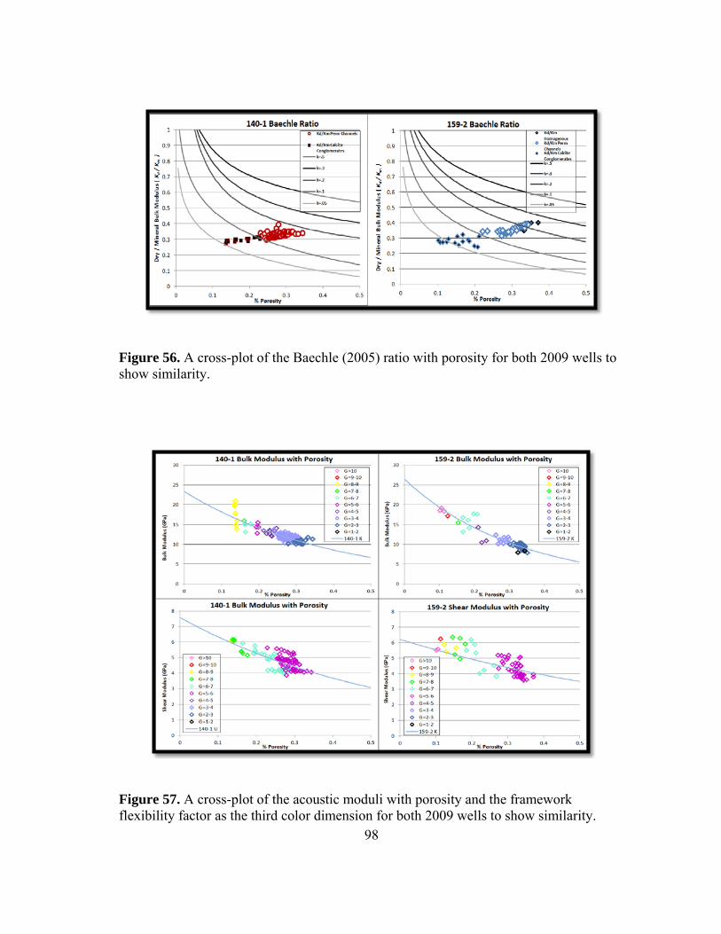
98

Figure 56. A cross-plot of the Baechle (2005) ratio with porosity for both 2009 wells to show similarity.

Figure 57. A cross-plot of the acoustic moduli with porosity and the framework flexibility factor as the third color dimension for both 2009 wells to show similarity.

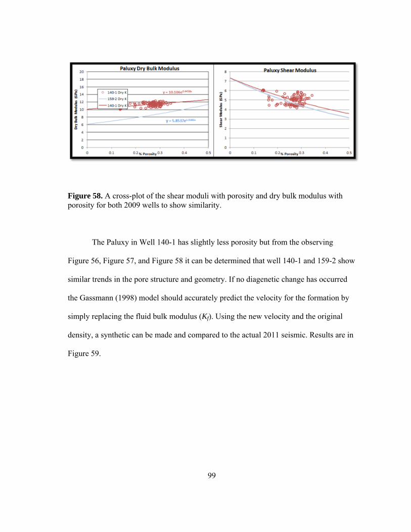
99

Figure 58. A cross-plot of the shear moduli with porosity and dry bulk modulus with porosity for both 2009 wells to show similarity.

The Paluxy in Well 140-1 has slightly less porosity but from the observing

Figure 56, Figure 57, and Figure 58 it can be determined that well 140-1 and 159-2 show

similar trends in the pore structure and geometry. If no diagenetic change has occurred

the Gassmann (1998) model should accurately predict the velocity for the formation by

simply replacing the fluid bulk modulus (Kf). Using the new velocity and the original

density, a synthetic can be made and compared to the actual 2011 seismic. Results are in

Figure 59.

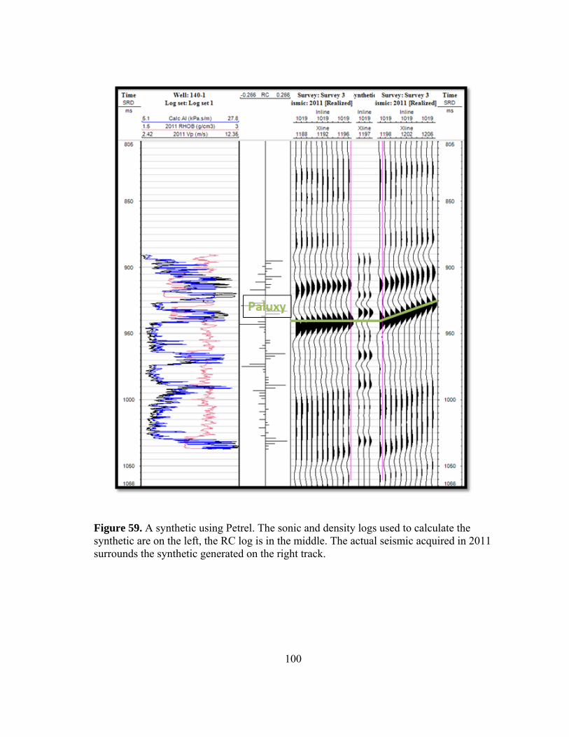
100

Figure 59. A synthetic using Petrel. The sonic and density logs used to calculate the synthetic are on the left, the RC log is in the middle. The actual seismic acquired in 2011 surrounds the synthetic generated on the right track.

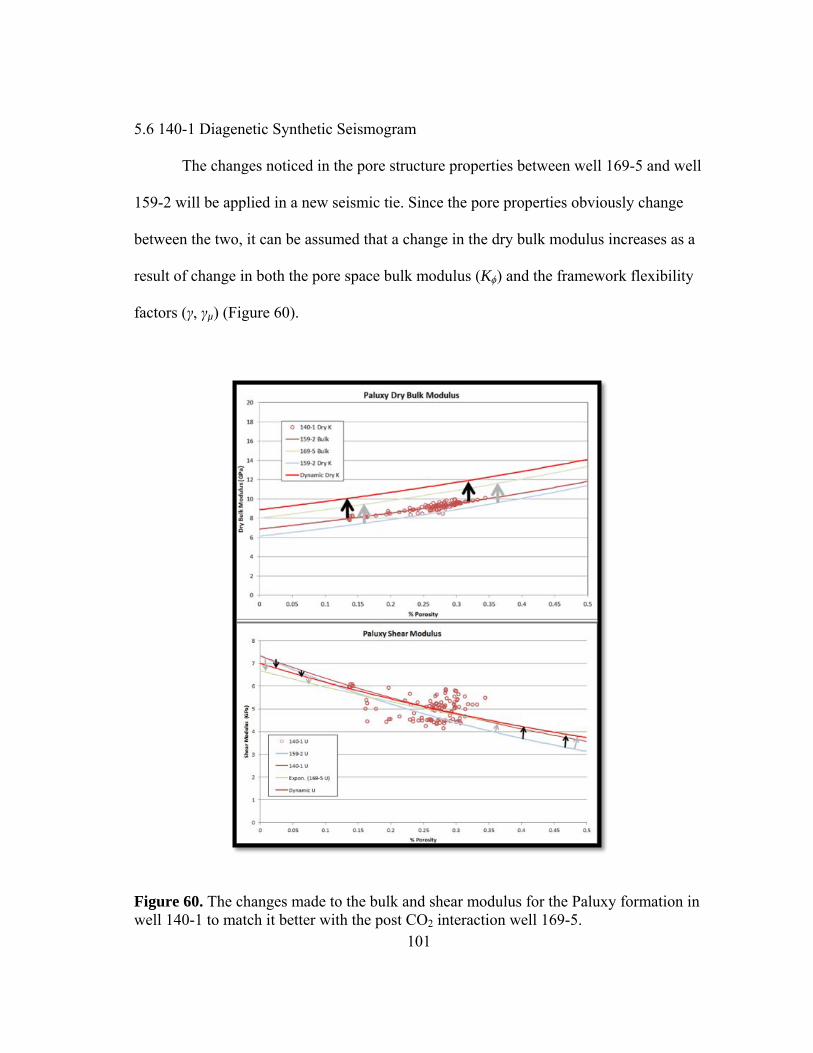
101

5.6 140-1 Diagenetic Synthetic Seismogram

The changes noticed in the pore structure properties between well 169-5 and well

159-2 will be applied in a new seismic tie. Since the pore properties obviously change

between the two, it can be assumed that a change in the dry bulk modulus increases as a

result of change in both the pore space bulk modulus (Kϕ) and the framework flexibility

factors (γ, γµ) (Figure 60).

Figure 60. The changes made to the bulk and shear modulus for the Paluxy formation in well 140-1 to match it better with the post CO2 interaction well 169-5.

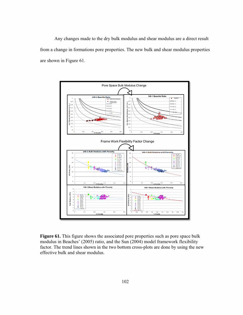
102

Any changes made to the dry bulk modulus and shear modulus are a direct result

from a change in formations pore properties. The new bulk and shear modulus properties

are shown in Figure 61.

Figure 61. This figure shows the associated pore properties such as pore space bulk modulus in Beaches’ (2005) ratio, and the Sun (2004) model framework flexibility factor. The trend lines shown in the two bottom cross-plots are done by using the new effective bulk and shear modulus.

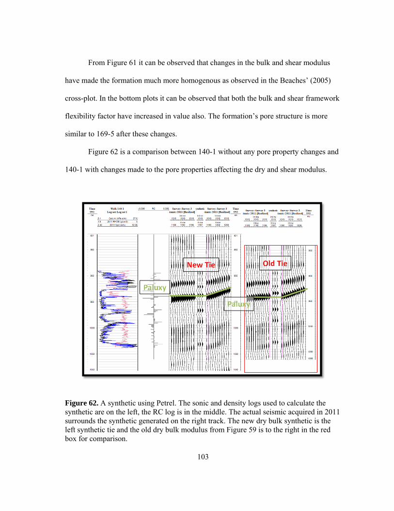
103

From Figure 61 it can be observed that changes in the bulk and shear modulus

have made the formation much more homogenous as observed in the Beaches’ (2005)

cross-plot. In the bottom plots it can be observed that both the bulk and shear framework

flexibility factor have increased in value also. The formation’s pore structure is more

similar to 169-5 after these changes.

Figure 62 is a comparison between 140-1 without any pore property changes and

140-1 with changes made to the pore properties affecting the dry and shear modulus.

Figure 62. A synthetic using Petrel. The sonic and density logs used to calculate the synthetic are on the left, the RC log is in the middle. The actual seismic acquired in 2011 surrounds the synthetic generated on the right track. The new dry bulk synthetic is the left synthetic tie and the old dry bulk modulus from Figure 59 is to the right in the red box for comparison.

104

The changes which were made to the bulk and shear modulus make a better tie to

the actual seismic. The changes in the dry bulk and shear modulus are associated with

changes made in the pore properties of the formation. This evidence concludes that the

pore properties of the Paluxy are actively changing within the reservoir during the CO2

injection

105

6. CONCLUSION AND DISCUSSION

6.1 Conclusion and Synopsis

• There was no evidence which suggest a large change in porosity or lithology

between the pre-CO2 injection 2009 well (159-2) or the post-CO2 injection 2010

well (169-5).

• There is an increase in permeability in the CO2 saturated 2010 well (169-5).

This permeability increase may be associated with a diagenetic effect during CO2

interaction.

• A relatively large increase in shear modulus in the post-CO2 injection 2010 well

(169-5) using shear sonic logs. This caused the p-wave velocity for the post-CO2

injection 2010 well (169-5) to increase as well.

• The change in velocity is quantified by the Baechle (2005) pore space bulk

modulus and the Sun (2004) formation flexibility factor in both wells.

• When using Gassmann (1998) equation to create a synthetic seismogram in well

140-1, a change to the dry bulk modulus and shear modulus ties better to the

2011 seismic acquisition.

• This evidence suggests that the Paluxy formation is chemically changing

6.2 Discussion of Future Rock Physics Work at Delhi

There is not thins sections for any well drilled post CO2 flood available, which

makes it hard to predict exactly what is happening to the pores. However, the thin

sections from 159-2 show many conglomerate calcified large grains with in the matrix.

These would cause the effects of heterogenetic reservoir porosity which was associated

106

with well 159-2. The CO2 most likely would dissolve the calcified cement holding these

conglomerate grains together. With thin sections from a recent well cored this hypothesis

could be proven. Also it would provide a better knowledge of what is happening at grain

boundaries after dissolution.

159-2 and 169-5 had other differences besides acoustic properties as noticed in

section 5.1. The other large difference between the two is the permeability between the

two. Whether this permeability is associated with the acoustic change in the reservoir

will be hard to determine, however, if a model using all the permeability logs in the area

was created and tested using different permeability scenarios a correlation to production

may be made. This is called a history match. The problem with this is there are a lot of

influential factors which create history match and more data about the reservoir would

need to be collected.

Well 169-5 showed a higher percentage of barite than the other two 2009 wells.

This could be because the solution is becoming oversaturated ad precipitating barite

instead of any calcite sediment because the brine water is sulfurous rather than

calcareous. A recent water sample would provide good evidence but thin sections from a

recent well would be better data.

107

REFERENCES

Avseth, P. (2011). "Rock Physics Modeling of Static and Dynamic Reservoir Properties-

a Heuristic Approach for Cemented Sanstone Reservoirs." The Leading Edge: 30 (1) 90-96. Baechle, G. T. (2005). "Changes of the Shear Moduli in Carbonate Rocks: Implications

for Gassman Applicability." The Leading Edge 24(1): 507-510. Baechle, G. T. (2009). "Changes in Dynamic Shear Moduli of Carbonate Rocks with Fluid Substitution." Geophysics 74(3): 135-147. Ballard, B. D. (2007). Quantitative Mineralogy of Reservoir Rocks Using Fourier Transform. Annual Technical Confrence and Exhibition. Anaheim, California, SPE. 113023-STU. Barrell, K. (1997). "Sequence Stratigraphy and Structural Trap Styles of the Tuscaloosa

Trend." Gulf Coast Association of Geological Societies Transactions 47: 27-34. Batzle, M. (1992). "Seismic Properties of Pore Fluids." Geophysics 57(11): 1396-1408. Bloomer Jr., P. A. (1946). “Subsurface Study of the Delhi Area Franklin and Richland Parishes Louisiana.” Baton Rouge, Department of Conservation Louisiana Geological Survey: 1-47. Brock, W. R. and L. A. Bryan (1989). “Summary Results of CO2 EOR Field Test 1972-1987.” Low Permeability Reservoirs Symposium. Denver, Colorado, SPE. 18977-MS: 499-508. Denbury Incorporation (2011). Corporate Responsibility Report. http://www.denbury.com/Corporate-Responsibility/company-overview/default.aspx, Denbury.com. DOE (2012). Enhanced Oil Recovery. http://energy.gov/sites/prod/files/eor_factcard.pdf

,

Fossil. Energy.gov. EIA (2011). International Energy Outlook 2011. http://www.eia.gov/. EIA. EPA (2012). Geologic Sequestration of Carbon Dioxide. http://water.epa.gov/type/groundwater/uic/wells_sequestration.cfm. EPA.gov. Eversull, L. (1985). "Depostional System and Distribution of the Cotton Vally Blanket Sandstones in Northern Louisana." Gulf Coast Association of Geological Societies Transactions 35: 49-58.

108

Evolution Petroleum Corporation (2008). Assets: CO2 EOR. evolutionpetroleum.com. Ewing, T. E. (2001). "Review of Late Jurassic Depositional Systems and Potential Hydrocarbon Plays, Northern Gulf of Mexico Basin." Gulf Coast Association of Geological Societies Transactions 51: 85-96. Han, D.-H. (2010). "CO2 Velocity Measurement and Models for Temperatures Up to 200 Degrees Celsius and Pressures Up to 100 MPa." Geophysics 75(3): 123-129. Hoffman, R. and Xu Y. (2005). "Effective Pressure or What is the Effect of Pressure?" The Leading Edge 24(12): 1256-1260. Hollingsworth, W. (1951). "Geophysical History of the Delhi Field, Richland, Franklin, and Madison Parishes, Louisiana." Geophysics 16(2): 185-191. Ikelle, L. and L. Amundsen (2005). Introduction to Petroleum Seismology. Tulsa, Okla., Society of Exploration Geophysicist. Kumar, D. (2005). "Pore Shape Effect on Elastic Properties of Carbonate Rocks." SEG Expanded Abstracts 24(1): 1477-1480. Lumley, D. (2010). "4D Seismic Monitoring of CO2 Sequestration." The Leading Edge 29(2): 150-155. Mammadova, E. (2011). “Influence of Rock Types on Seismic Monitoring of CO2 Sequestration in Carbonate Reservoirs.” Geosciences. College Station, Texas A&M University. Master of Science: 102. Mancini, E. A. (2008). "Sequence-Stratigraphic Analysis of Jurassic and Cretaceous Strata and Petroleum Exploration in the Central and Eastern Gulf Coastal Plain, United States." AAPG Bulletin 92(12): 1655-1686. Mancini, E. A. (1999). Basin Analysis of the Mississippi Interior Salt Basin and Petroleum System Modeling of the Jurassic Smackover Formation, Eastern Gulf Coastal Plain.” U.S. Department of Energy 1999 Oil and Gas Conference. Tulsa, Oklahoma, DOE. 1 and 2: 1-343. Mancini, E. A. and T. M. Puckett (2002). “Transgressive-Regressive Cycles: Application to Petroleum Exploration for Hydrocarbons Associated with Cretaceous Shelf Carbonates and Coastal and Fluvial-Deltaic Siliciclastics, Northeastern Gulf of Mexico.” 22nd Annual Gulf Coast Section SEPM Foundation Bob F. Perkins Research Conference, SEPM. 1: 173-199.

109

Mavko, G. (2009). The Rock Physics Handbook : Tools for Seismic Analysis of Porous Media. Cambridge, UK ; New York, Cambridge University Press. Mohapatra, A. (2012). “Seismic Signature of Sedimentary Rocks with CO2 Flooding: Thesis, University of the Oklahoma.” Petroleum and Geological Engineering. Norman, Unversity of Oklahoma. Master of Science. Muller, T. (2010). "Seismic Wave Attenuation and Dispersion Resulting from Wave-Induced Flow in Porous Rocks." Geophysics 75(4): 147-164. Patterson, O. (1956). "The Determination of the Water-Injection Program for the Delhi Field by Means of the Automatic Multi-Pool Analyzer." Petroleum Transactions, 207(1): 73-79. Powell, J. (1972). Exploration History of Delhi Field, Northeastern Louisiana. Stratigraphic Oil and Gas Fields – Classification, Exploration Methods, and Case Histories. R. E. King, AAPG Special Volumes. M 16: 548-558. Preston, C. (2005). "IEA GHG Weyburn CO2 Monitoring and Storage Project." Fuel Processing Technology 86(1): 1547-1568. Robin, P.-Y. (1973). "Note on Effective Pressure." Journal of Geophysical Research 78(14): 2434-2437. Silvis, N. (2011). “Reservoir Characterization to Determine Tertiary CO2 Flow Paths in the Holt-Bryant Reservoir, Delhi Field, Northeastern Louisiana.” Geoscience. Golden, Colorado, Colorado School of Mines. Master of Science. Society for Sedimentary Geology (2013). “Tide Wave Dominated Deltas.” http://www.sepmstrata.org/page.aspx?pageid=313. SEPMstrata.org. Geophysics Study Committee, Geophysics Research Forum, National Research Council. (1986). Active Tectonics:Impact on Society, Publication of the The National Academies Press. Washington, D.C. Stalkup, F. I. (1978). "Carbon Dioxide Miscible Flooding: Past, Present, and Outlook for the Future." Journal of Petroleum 30(8): 1102-1112. Sun, Y. F. (2004). "Pore Structure Effect on Elastic Wave Propagation in Rocks: AVO Modeling." Journal of Geophysics and Engineering 1(4): 42-49. Eschner, Terry (2009) "Conventional and Advanced Core Analysis for Well 159-2, Delhi, LA." Core Lab. Houston , TX.

110

Vanorio, T. (2010). "The Rock Physics Basis for 4D Seismic Monitoring of CO2 Fate: Are We There Yet?" The Leading Edge 29(2): 156-162. Warner, D. L. and C. L. McConnell (1993). "Assessment of Environmental Implications of Abandoned Oil and Gas Wells." Society of Petroleum Engineers SPE 20692: 874-880. Wolcott, J. M. (1989). The Effects of CO Flooding on Reservoir Mineral Properties. SPE International Symposium on Oilfield Chemistry, Houston, Texas, Society of Petroleum Engineers. Wyllie, M. (1956). "Elastic Wave Velocities in Heterogeneous and Porous Media." Geophysics 21(1): 41-70. Wyllie, M., Gregory, A., and Gardner, G. (1958). "An Experimental Investigation of Factors Affecting Elastic Wave Velocities in Porous Media." Geophysics 23(4): 459-493. Yuh, S. (2004). “Time-Lapse Seismic Monitoring of Subsurface Fluid Flow.” Geophysics. College Station, Tex., Texas A&M University. Master of Science: 103.