“A Robust Time-varying Style Analysis for Hedge … · “A Robust Time-varying Style Analysis for Hedge Funds based on Dynamic Quantiles ... analysis framework remains static whereas

“A Robust Time-varying Style Analysis for Hedge Funds

based on Dynamic Quantiles”∗

Benjamin Hamidi† Bertrand Maillet‡ Paul Merlin§

February 2011

Abstract

In the original approach by Sharpe (1992), style analysis aims to explain portfolio per-formances according to the fund exposure to a set of asset classes. Typically, multivariateregression is involved to obtain the fund sensitivity to various benchmarks. However, thisapproach has been criticized because of the non-robustness of the estimation. Moreover, theanalysis framework remains static whereas fund allocation could be dynamic.To remedy to these drawbacks, we propose a robust time-varying global estimation involvingQuantile Regression. The advantage of the Quantile Regression is that the whole shape of thedistribution is taken into account rather than the simple mean in the case of OLS. Moreover,Quantile Regression is a robust statistical method that gives less weight to “outliers”. Wepropose a new time-varying framework for quantile regression in order to capture the dynamicstyle allocation. Our robust approach is finally applied to the main hedge fund strategy indexesfrom HFR.

Keywords: Style Analysis, Quantile Regression, L-estimator, FLS, Hedge Funds, Time-

varying.

JEL Classification: C14, C22, C29, G11.

∗We thank Thierry Chauveau, Gilbert Colletaz, Jean-Michel Zakoıan and Patrick Kouontchou for their kind help and

advices. The second author thanks the Europlace Institute of Finance for financial support. Preliminary draft: do not quote

or diffuse without permission. The usual disclaimer applies.†A.A.Advisors-QCG (ABN AMRO), Variances and University of Paris-1 (CES/CNRS). E-mail: benjamin.hamidi@univ-

paris1.fr‡A.A.Advisors-QCG (ABN AMRO), Variances and University of Paris-1 (CES/CNRS and EIF). Corresponding author:

Dr B. B. Maillet, CES/CNRS, MSE, 106-112 Bd de l’Hopital F-75647 Paris Cedex 13. Tel: +33 144078189/70 (fax). Email:

[email protected].§A.A.Advisors (ABN AMRO) and University of Paris-1 (CES/CNRS). E-mail: [email protected]

1

“A Robust Time-varying Style Analysis for Hedge Funds

based on Dynamic Quantiles”

February 2011

Abstract

In the original approach by Sharpe (1992), style analysis aims to explain portfolio per-formances according to the fund exposure to a set of asset classes. Typically, multivariateregression is involved to obtain the fund sensitivity to various benchmarks. However, thisapproach has been criticized because of the non-robustness of the estimation. Moreover, theanalysis framework remains static whereas fund allocation could be dynamic.To remedy to these drawbacks, we propose a robust time-varying global estimation involvingQuantile Regression. The advantage of the Quantile Regression is that the whole shape of thedistribution is taken into account rather than the simple mean in the case of OLS. Moreover,Quantile Regression is a robust statistical method that gives less weight to “outliers”. Wepropose a new time-varying framework for quantile regression in order to capture the dynamicstyle allocation. Our robust approach is finally applied to the main hedge fund strategy indexesfrom HFR.

Keywords: Style Analysis, Quantile Regression, L-estimator, FLS, Hedge Funds, Time-

varying.

JEL Classification: C14, C22, C29, G11.

2

“A Robust Time-varying Style Analysis

based on Dynamic Quantiles”

1 Introduction

A typical style analysis aims to determine the sensibility of a fund to a set of factors. The

emergence and the success of style analysis probably come from the fact that various ap-

plications can be proposed from the knowledge of these sensibilities. For an investor, style

analysis provides him a better understanding of the fund strategy and its sources of returns.

For a fund manager, reference to a specific style leads to a more precise definition of his

strategy. It can allows him to define an ad hoc benchmark. This is a reason why style

analysis is widely used in performance analysis and asset management.

Two main approaches have been proposed when assessing the global style of a portfolio

(ter Horst et al., 2004). The first one refers to Holding-based Style Analysis (HBSA) and

consists in the style determination of every asset in the portfolio before aggregating them to

get the overall style of the portfolio. The second one, often called Return-based Style Analy-

sis (RBSA), was introduced by Sharpe (1988 and 1992). This paper mainly considers RBSA.

Such models have been jointly developed with asset pricing models. The first attempts to

compare funds have used the Capital Asset Pricing Model (CAPM, Sharpe 1964). The main

drawback of single factor models (for instance CAPM) is that they are too restrictive since

in most cases, more than one systematic risk factor is needed to describe returns; this is

particularly true considering hedge funds with different styles (taking long or short positions

on different markets1). Consideration of linear multi-factorial models has been proposed to

overcome these limits. With the introduction of the Asset Pricing Theory (APT) by Ross

(1976), a new generation of multi-factorial models has appeared.

1The main hedge fund strategies are briefly presented in the appendix.

3

The big issue with multi-factorial models lies with the choice of factor and the so called

selection bias. Indeed, without enough knowledge on the investment strategy followed by the

fund manager, one can miss an important factor; the obtained style analysis could then be

biased. For this last approach, the choice of factors is of critical importance. Factor reduc-

tion techniques (Principal Component Analysis or Independent Component Analysis) have

been proposed to obtain relevant factors without any a priori on a fund strategies. From a

large set of fund performances these methods aim to extract a small number of independent

(at least uncorrelated) variables. These approaches have the advantage of complying with

some of the statistical hypothesis required by the considered model but the obtained factors

are virtual (they did not correspond to real asset performances) and associated sensibilities

are hardly interpretable.

The second class of models uses real assets as factors. Stylized facts such as the “value

premium” for equity portfolios have lead to the introduction of ad hoc factors. For instance,

Fama and French (1993) proposed an expanded three-factor model that considers the market

exposure factor, the SMB size factor (denoting Small Minus Big) and a variable depending

on the stock’s book-to-market, HML (denoting High book to price Minus Low book to

price). The existence of a price momentum effect was documented by Jegadeesh and Titman

(1993). It reflects strategies that consist in buying stocks which have well performed in the

past and selling stocks which have historically performed poorly. Carhart (1997) proposed

to integrate a momentum factor (denoting WML for Winners Minus Losers) in the so-called

Carhart model (1997). But these methods require corrections for drawing inferences (as the

model contains inequality constraints). The estimation suffers from the presence of outliers

(Chan and Lakonishok, 1992) because it is essentially based on a Least Square estimation

procedure.

Hedge funds have received a vast amount of attention over the last decades. They are car-

acterized by a great opacity regarding their investment strategies. They differ significantly

from traditional investments, such as mutual funds, due to the lack of strong regulation on

this asset class. Hedge fund managers enjoy a great flexibility in their investments (dynamic

asset allocations, leverage, short-selling, derivatives etc). There exist various hedge fund

4

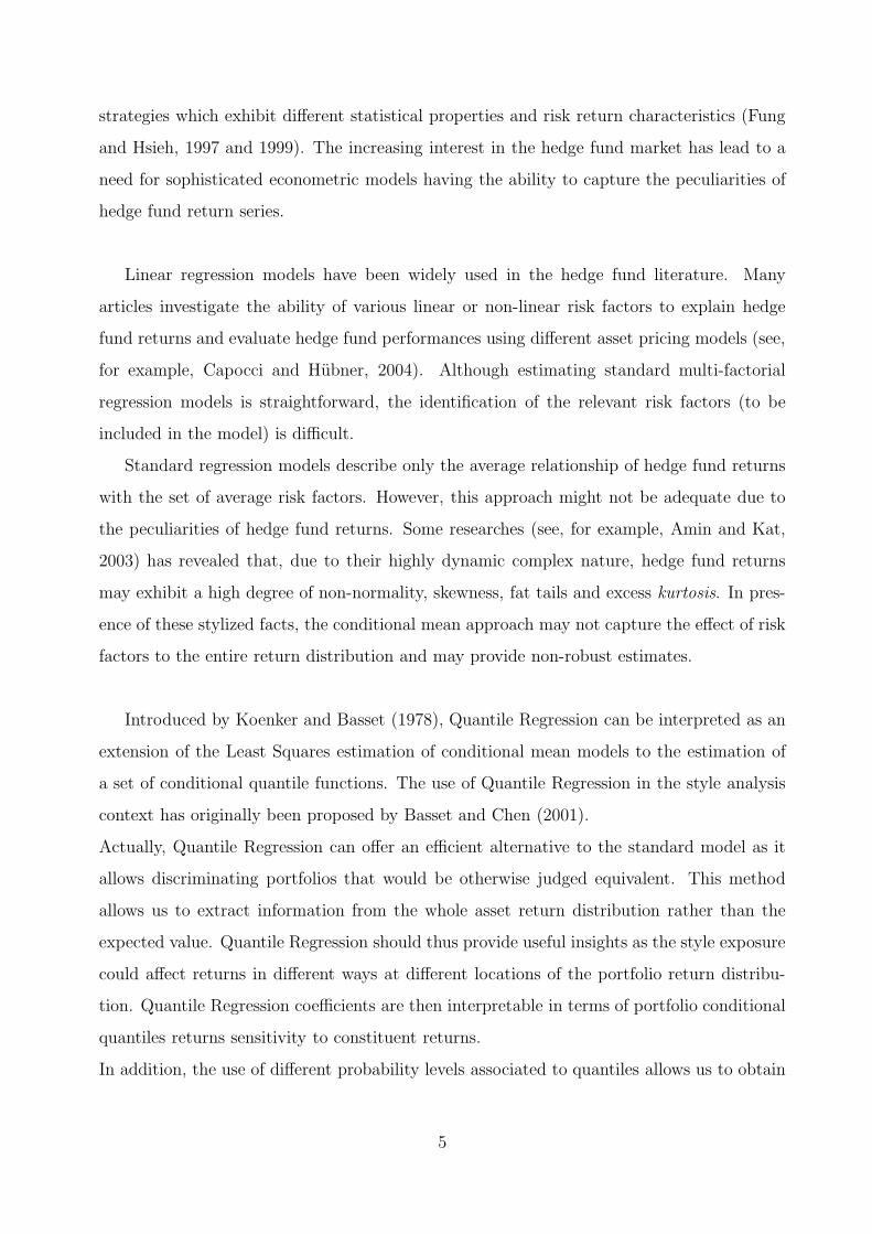
strategies which exhibit different statistical properties and risk return characteristics (Fung

and Hsieh, 1997 and 1999). The increasing interest in the hedge fund market has lead to a

need for sophisticated econometric models having the ability to capture the peculiarities of

hedge fund return series.

Linear regression models have been widely used in the hedge fund literature. Many

articles investigate the ability of various linear or non-linear risk factors to explain hedge

fund returns and evaluate hedge fund performances using different asset pricing models (see,

for example, Capocci and Hubner, 2004). Although estimating standard multi-factorial

regression models is straightforward, the identification of the relevant risk factors (to be

included in the model) is difficult.

Standard regression models describe only the average relationship of hedge fund returns

with the set of average risk factors. However, this approach might not be adequate due to

the peculiarities of hedge fund returns. Some researches (see, for example, Amin and Kat,

2003) has revealed that, due to their highly dynamic complex nature, hedge fund returns

may exhibit a high degree of non-normality, skewness, fat tails and excess kurtosis. In pres-

ence of these stylized facts, the conditional mean approach may not capture the effect of risk

factors to the entire return distribution and may provide non-robust estimates.

Introduced by Koenker and Basset (1978), Quantile Regression can be interpreted as an

extension of the Least Squares estimation of conditional mean models to the estimation of

a set of conditional quantile functions. The use of Quantile Regression in the style analysis

context has originally been proposed by Basset and Chen (2001).

Actually, Quantile Regression can offer an efficient alternative to the standard model as it

allows discriminating portfolios that would be otherwise judged equivalent. This method

allows us to extract information from the whole asset return distribution rather than the

expected value. Quantile Regression should thus provide useful insights as the style exposure

could affect returns in different ways at different locations of the portfolio return distribu-

tion. Quantile Regression coefficients are then interpretable in terms of portfolio conditional

quantiles returns sensitivity to constituent returns.

In addition, the use of different probability levels associated to quantiles allows us to obtain

5

a set of conditional quantile estimators. The latter can be linearly combined in order to

construct a L-estimator which then gives rise to a gain in efficiency (Koenker and Portnoy,

1987).

Fund style management is often active, time-varying and depends on market opportunities

(Fung et al., 2008; Kosowski et al., 2007; Jagannathan et al., 2010). Bollen and Whaley

(2009), propose an optimal change point regression and a stochastic beta model to estimate

changes in hedge fund risk dynamics. Billio et al. (2010) measure the dynamic risk exposure

of Hedge Funds to various risk factors during different market volatility conditions using

a regime-switching beta model. Finally, a new time-varying framework based on quantile

dynamics can be defined for a better assessement of fund active style management.

The main goal of this paper is to provide and estimate a robust time-varying multi-

quantile framework for style analysis. The second section of this paper is devoted to a brief

review of style analysis problematics, evolutions and the critical step of the factor selection.

We propose to use peer group analysis to select the factors that will be used to investigate

hedge fund styles. After having recalled the traditional OLS and Quantile Regression frame-

work, we propose to adapt the Time-varying Flexible Least Square approach to L-estimators

based on a Quantile Regression. We thus introduce the time-varying multi-quantile robust

approach for style analysis. The fourth section illustrate this robust time-varying approach

on hedge fund strategies as defined in the HFR database on monthly data from January

1995 to January 2010. The last section concludes.

2 Style Analysis Approaches

Style analysis stands nowadays out as a major reference in portfolio management. Given that

the large variety of management offers, style analysis has become fundamental to decompose

and justify performance differences between funds belonging to the same asset class. A vast

literature is dedicated to this subject. Several approaches are proposed to estimate the style

associated to a fund. In this article, we suppose that a style is defined according to the

risk factors to which the fund is exposed. The fund sensibility to risk factors allows us to

estimate the future expected returns and verify the coherence of the performances given the

6

fund objectives.

In this section, we first set the general style analysis framework, then we describe the prob-

lematic linked to the critical choice of the risk factors. At last, we propose to use a peer

group analysis to select among a benchmark universe relevant factors in our robust style

analysis framework dedicated to hedge funds.

2.1 Style Analysis Evolution

Style analysis models evolved together with asset evaluation models. Thus, the first attempt

of grouping funds uses the systematic risk of the Capital Asset Pricing Model (CAPM;

Sharpe, 1964). Since the apparition of the Asset Pricing Theory (APT) by Ross (1976), a

new generation of multi-factorial models has been developed. Besides the choice of statisti-

cal methods, style analysis models mostly differ from the choice of factors. The definition

of the factors is clearly influenced by the observation of market abnormalities. Numerous

studies conclude to the existence of a capitalisation bias in equity returns (Lakonishok and

Shapiro, 1986). Others (Lakonishok et al., 1994; Fama and French, 1998, for example) show

that the Book-to-Market ratio (B/M) should be taken into account for return estimations.

These abnormalities give rise to the introduction of four traditional explanatory factors: the

styles Growth, Value, Large and Small. If the precise definitions of the styles Large and

Small are immediate, the ones of the styles Growth and Value are more uncertain. Roughly,

the style Growth characterizes the companies with a significant anticipated organic growth.

A Value investment strategy consists in buying securities that are considered underestimated.

For portfolio style analysis, two widely spread approaches have been proposed. The

first one, called the Holding-Based Style Analysis (denoted HBSA, Cf. Daniel et al., 1997)

consists in the analysis of every holding compounding the portfolio. The aggregation of these

obtained styles allows us to assess the global style of the portfolio studied. Such an approach

requires a large amount of information (breakdown of the portfolio, a forecast ratio and

other peculiarities of each holding for instance) and is hard to set up in practice. Moreover,

when dealing with hedge funds, the traditional opacity on the investment strategies makes

the HBSA potentially unfeasible.

7

An alternative to the HBSA is found in the Return-Based Style Analysis (denoted RBSA);

the goal of this approach is to measure the sensibility of a portfolio onto a set of factors.

The seminal work of Sharpe (1988 and 1992) follows a statistical approach to estimate these

sensibilities and evaluate the global style of a fund. This approach is hereafter developed

in this paper. Thus, style analysis model regresses portfolio returns on the ones of the N

constituents, such as:

RP[T×1]

= α 1(T×1)[T×1]

+ F[T×N ]

BC[N×1]

+ e[T×1]

, (1)

where RP is the vector of portfolio returns over time, F the matrix containing the returns

over time of the risk factors (portfolio constituents), α and BC = (β1, ..., βN)′ are estimated

constrained parameters, e = (ε1, ..., εT )′ is the vector of residuals and data are observed on

T subsequent time periods.

The Principal Component Analysis (PCA), the Independent Component Analysis (ICA)

and the Kohonen Self-Organizing Maps (SOM) classification are three different ways of con-

sidering the multi-factorial approach presented in equation (1). This methods allow us to

express the factors as a portfolio of assets defined by weights, such as (with the previous

notations):

F[T×N ]

= R[T×N ]

Wx[N×N ]

(2)

where R is the (T × N) matrix of returns, Wx with x = [PCA, ICA, SOM] stand for WPCA,

WICA and WSOM which are respectively the extraction matrices associated to PCA, ICA

and SOM methodologies.

Within the PCA the matrix of linear independent factors can be expressed such as:

WPCA = ArgmaxWPCA

E{

(RWPCA)2}

(3)

where R is the (T × N) matrix of assets returns, WPCA is the eigenvectors associated to

the matrix RR′, with R′ the transpose of R.

8

PCA aims to find linear combinations of returns (i.e. portfolio return time-series) that

most explain the global volatility of the underlying assets returns, under the constraint of

null-covariances between returns of built factors. The goal of the PCA is therefore to remove

second-order dependencies in the data. If higher order dependencies exist between the vari-

ables then removing second-order dependencies is insufficient at revealing all structure in the

data. Multiple solutions exist for removing higher-order dependencies. For instance, we can

transform the data to a more appropriate naive basis. However, in the context of returns

decomposition, outliers can be difficult to identify. PCA has been applied to the analysis

of hedge funds (Fung and Hsieh, 1997 and 1999), however, the PCA model generated low

levels of cross sectional variation in hedge fund returns.

Another method of factorial decomposition, the Independent Component Analysis (ICA, see

Hyvarinen et al., 2001) is to impose more general statistical definitions of dependency within

a data set: requiring that data along reduced dimensions are statistically independent. This

class of algorithms has been demonstrated to succeed in many domains where PCA fails.

ICA aims to find linear combinations of returns so that factors are independent grouping

asset returns in a class whose representatives are weighted sums of asset return time-series

(with weights depending on a distance between the asset return time-series). An application

of ICA to explain the factors driving the hedge fund returns can be found in Olszewski

(2006). The ICA allows us to express a set of multidimensional observations as a combina-

tion of unknown latent variables. These unknown latent variables are called “sources” or

“independent components” and are supposed to be statistically independent. To extract the

factors you have to get the extraction matrix denoted WICA, such as (with the previous

notations):

WICA = ArgmaxWICA

NG[WICA(R − α)

], (4)

where NG(.) is a function which measures the non Gaussianity of the returns.

The difference between PCA and ICA that is relevant to hedge funds is that while PCA al-

gorithms use only second order statistical information, ICA algorithms may use higher order

statistical information for separating signals. For this reason non-Gaussian signals (or at

most, one Gaussian signal) are required (Back and Weigend, 1997) and measured by NG(.).

9

Kohonen Self-Organizing Maps (SOM) can be used at the same time both to reduce the

amount of relevant data by clustering, and for projecting the data non-linearly onto a lower

dimensional display. This iterative algorithm has been applied to Hedge Fund classification

by Maillet and Rousset (2003). Factors are determined iteratively and adapt theirselves

during the SOM algorithm. The w(i,j)SOMcomponents of the WSOM matrix can be iteratively

determined such as (with the previous notations):

w(i,j)SOM= w(i−1,j)SOM

− εi−1Λ (BMUi,Fj)[w(i−1,j)SOM

− 1], (5)

with:

BMUi = ArgminFj ,j∈I

{∥∥Ri,j − F(i−1,k)

∥∥}, (6)

where εt is the adaptation gain parameter, which is ]0, 1[-valued, generally decreasing with

time. The number of neurons taken into account during the weight update depends on the

neighborhood function Λ that also decreases with time and ‖.‖ is the Euclidean norm.

Most of RBSA models consider a (multi-) factorial approach to model returns and assess

the portfolio style. This class of models must have three main desirable properties. First,

parameters (sensibility to factors) should be estimated robustly and in a reasonable amount

of time. Secondly, an intuitive interpretation has to be provided (factors are real assets for

instance). Thirdly, the model has to be parsimonious in terms of involved factors (leads to

a robust estimation).

2.2 Style Analysis Approach for Hedge Funds

In front of the reproduction of the empirical works indicating that the other variables explain

the excedentary returns and to the difficulty validating the CAPM (for example, Lakonishok

and Shapiro, 1986; Chopra and Ritter, 1989; Fama and French, 1992), the evaluation models

evolved towards the consideration of others risk factors than the only market risk.

The APT model, introduced by Ross in 1976, supposes that asset returns are influenced by

various (macroeconomic) exogeneous factors. The expected return of a portfolio is a function

depending on a basket of explanatory factors and on the fund sensibilities with regard to

these risk factors. To be valid, these models require to have independent factors. Indeed,

10

the collinearity between these factors can lead to a spurious regression and thus infer in the

determination of the sensibilities. To suit these statistical constraints, methods of factorial

decomposition were proposed. Ross uses the Principal Component Analysis (PCA) to iden-

tify linearly independent factors. Under the hypothesis of normality of asset returns, the

main constituents are also independent. The determination of the fund exposure onto the

principal orthogonal factors (avoiding the drawbacks of multi-collinearity) is therefore made

possible.

If higher order dependencies exist between the variables then removing second-order de-

pendencies the PCA is insufficient at revealing all structure in the data. Another method of

factorial decomposition, the Independent Component Analysis (ICA, see Hyvarinen et al.,

2001), enables to drop this hypothesis. The ICA allows us to express a set of multidimen-

sional observations as a combination of unknown latent variables. These unknown latent

variables are called “sources” or “independent components” and are supposed to be statis-

tically independent. The independence is estimated here beyond the moment of order 2 and

integrated directly into the optimization function (Cf. Chap and Robin, 2008).

Whatever the factorial decomposition method is chosen, two main issues remain. The imple-

mentation of these models requires a priori knowledge on the factors to which the considered

fund is exposed. The risk factors being abstracted, the interpretation of the fund sensibilities

to these factors is not always easy.

Sharpe (1988 and 1992) presents a model adopting this time an approach relative to the

APT framework. He considers that the bets and strategies of a manager (preference for an

asset class or a given sector) are going to define the style of the manager. The hypothesis of

the Sharpe style model is that differences of behavior are going to be echoed directly on the

managed funds returns. He uses real factors of the economy and considers a basket of mar-

ket indicators (shares, bonds). By means of a multivariate regression under constraints, he

determines the sensibilities of the fund to the factors. In spite of the choice of the representa-

tive benchmarks and the problems of statistical order connected to the potential collinearity

of the used factors, this model became a reference in style analysis. Besides, the use of real

factors leads to a direct interpretation of the implemented strategies by the manager.

11

About representative factors of hedge fund strategy, it is reasonable to assume that the

risk sources associated with hedge funds are fairly similar to those associated with tradi-

tional assets. Multi-factorial models for hedge fund analysis have been proposed (see for

instance, Schneeweis and Spurgin, 1999; Schneeweis et al., 2002; and Capocci and Hubner,

2004). Some of these factors are: equity related factors (market or sector index, traded

volume...), equity trading styles (Fama and French factors) or interest rate factors (T-bill

rate, slope of the yield curve, credit risk premium...). In the empirical part of this work, we

model the hedge fund returns by using different information variables and pricing factors in

the lines of Agarwal and Naik (2000 and 2004). Thanks to a clustering method based on a

peer group analysis, we select the relevant factors among a benchmark database, composed

initially by: equity related factors (the Russel 3000 equity index, the MSCI World excluding

the USA, the MSCI Europe-EMU, the MSCI Emerging Market index, the MSCI Emerging

Market excluding Asia, the TOPIX), equity trading styles (Carhart and Fama and French

factors on the US; Small Minus Big - SMB, High Minus Low - HML, Momentum factor,

Long-term and Short-term reversal factors), interest rate factors (the US LIBOR 3 Months,

the 10 Year Treasury rate, the J.P. Morgan U.S. Aggregate Bond Index, the J.P. Morgan

EMU all maturities, the credit Suisse High Yield index), Commodity factors (the S&P global

commodity index and the CRB All Commodities), and a factor linked to derivatives (the

evolution of equity Implied Volatility Index - VIX).

Some results show that an HBSA approach does not infer better results that the RBSA

approach (ter Horst et al., 2004). Although this model is widely spread, it is the object

of severe criticisms. The fact that the considered factors are generally strongly collinear

constitutes one of them; because any regression on these risks to be fuzzy. The standard

RBSA models presented until suffer from two major limits.

The analysis is static; the fund exposure to factors are supposed constants over the time.

For a fund managed passively, this approach is valid. But since we consider funds adopting

an active management, a static setting is not anymore viable.

The second criticism is connected to the necessity of specifying a priori the risk factors.

A preliminary knowledge of the analyzed funds is required to choose factors. For instance,

Sharpe (1988) chooses real economic factors (equities and bonds benchmarks) without in-

12

tegrating the styles Growth, Value, Large and Small. It is necessary to wait for the three

factors model of Fama and French (1998) to consider these last ones.

Brown and Goetzmann (1997) adopt an original approach. Exploiting the strong link be-

tween factorial analysis methods and classification algorithms, they suggest collecting funds

in homogeneous groups. For each of these groups is identified a risk factor (defined as the

average of the funds of each group). This model, easy to implement, has a strong explanatory

power. Indeed, factors arising from the universe of funds, it is not necessary to know a priori

the styles. The bias, even if they were not observed yet, will be directly integrated into the

risk factors. Factors being determined directly from the funds, this model allows us to obtain

risk factors reflecting, among others, the active management strategies. Adopting a similar

approach, Maillet and Rousset (2003) and Aaron et al. (2004) suggest to analyze the style

of funds by exploiting a classification method called Kohonen Self-Organizing Maps (SOM).

This algorithm allows the simultaneous determination of the homogeneous groups of funds,

and the risk factors. An advantage of the maps of Kohonen by report to the algorithm which

was used by Brown and Goetzmann (1997), is the preservation of the topology. The rep-

resentative factors of the groups of funds are ordered on the map according to their similitude.

Following this field of the literature, we use the Self-Organizing Maps (Kohonen, 2000) to

build a more robust style analysis model, selecting appropriate benchmarks (factors) in our

approach. The method of classification, SOM allows the simultaneous generation of specific

risk factors and homogeneous groups of strategies and benchmarks.

2.3 Factors for Style Analysis

To perform our robust style analysis approach, we use the Kohonen approach to analyze a

set of risk factors and avoid to get “dependent” explanatory variables.

The algorithm of the Kohonen map allows us to obtain non linear classifications without

any a priori on data to classify. Various financial applications of SOM were proposed: from

the simple exploration of fund universe, to the forecast of future returns. In spite of its ro-

bustness, the stochastic property of the algorithm can be subject to convergence problems.

13

We thus choose a robust version of the Kohonen map (Guinot et al., 2006). We briefly

recall hereafter (details are provided in the appendix 6.2), the SOM algorithm and its robust

version. We show then, how the robust map can be used within the framework of a style

analysis model.

We briefly present herein the data mining technique we apply for grouping together

elements (hedge fund track records and factors for instance)2. Self-Organizing Map is a

clustering method belonging to Artificial Neural Networks. SOM can be used at the same

time both to reduce the amount of relevant data by clustering, and for projecting the data

non-linearly onto a lower dimensional display. Due to its unsupervised learning and topology

preserving properties, the SOM algorithm has proven to be especially suitable in visual

analysis of high dimensional sets. They have already been applied in various fields in general,

and in finance in particular, for clustering elements sharing some similarities. Without any

pretension of exhaustivity, some examples of SOM financial applications are to be found

in Deboeck and Kohonen (1998), Resta (2001), Maillet and Rousset (2003), Moreno et

al. (2006), and Ben Omrane and de Bodt (2007). For further details on this data-mining

technique, see Kohonen (2000) and Guinot et al. (2006).

The SOM is a method that represents statistical data sets in an ordered way as a natural

groundwork on which the distributions of the individual indicators in the set can be displayed

and analyzed. It is based on the unsupervised learning process where the training is entirely

data-driven and no information about the input data is required (see Kohonen, 2000).

The SOM consists3 of a network, compound of n neurons, units or code vectors organized

on a regular low-dimensional grid. If I = [1, 2, ..., n] is the set of units, the neighborhood

structure is provided by a set of neighborhood function Λ defined on I2. The network state

at time t is given by:

m (t) = [m1 (t) ,m2 (t) , ...,mn (t)] , (7)

where mi (t) is the T -dimensional weight vector of the unit i.

For a given state m and an input x, the winning unit iw (x,m) is the unit whose the weights

miw(x,m) is the closest to the input x.

If the quality of SOM classifications is generally satisfactory, the stochastic property of the

2An illustration of the algorithm is provided in Figure (16) of the appendix3The SOM algorithm is presented in the appendix.

14

algorithm does not guaranteed the systematic convergence of the classification. Since two

successive SOM learning may not provide the same results, a model risk can arise when using

a simple Kohonen algorithm to develop style model. To avoid such convergence problems,

we apply a modified version of the Kohonen algorithm as proposed by Guinot et al. (2006):

robust maps (Robust Self-Organizing Maps, RSOM). To limit the network dependences to

the learning data model, it is classic to apply a Bootstrap process with resampling tech-

niques.

The Bootstrap technique is applied here to the SOM by estimating a probability for every

individual being in the same group. This probability is empirically estimated during the

SOM learning step performed on the resampled temporal series.

The classification algorithm uses only the individuals present in the resampled database

(60 % of the original individuals). We generalize this approach by adding an edition with-

out replacement of the observations (60 % of the original observations). At the end of

the first step, individuals spread during the process of re-sampling are classified from their

distances in vector codes. So, in every stage of the classification, we obtain the probability

to be in the same group for every individual (including those spread during the re-sampling).

Thus, we perform the Robust SOM classification onto the benchmark universe (presented

above) and the main HFR strategies and we try to select one risk factor per group to limit

“dependencies” between risk factors.

3 About Style Analysis Modeling

In this section, after having recalled the traditional Least Square and Quantile Regression

framework, we propose to adapt the Time-varying Flexible Least Square approach to L-

estimators based on Quantile Regression. We thus introduce the time-varying multi-quantile

robust approach for style analysis.

3.1 Least Square Constrained Regression Models

The classical model is based on a constrained least square regression model (see Sharpe 1988

and 1992).

The use of a Least Square model focuses on the conditional expectation of portfolio re-

15

turn distribution. It can be formulated as follows (with the previous notations):

E(RP |Ft) = α + FtBC . (8)

Estimated compositions are then interpretable in terms of sensitivity of portfolio expected

returns to constituent returns. In the classical regression context, the βi coefficient represents

the impact of a change in the returns of the ith constituent on the portfolio expected returns,

holding the values of the other constituent returns constant. Using the Least Square model,

portfolio style is then determined by estimating the style exposure influence on expected re-

turns. Although the estimated Least Square coefficients are in common practice interpreted

as a composition at the last time, it is worthwhile stressing that they reflect the average

effect over the time period studied, according to the regression framework. Estimated Least

Square coefficients are to be compared to average portfolio composition. Even if the Least

Square framework has been sometimes presented within a dynamic estimation method (using

for example a rolling window of returns to perform estimations), it can not be considered as

a real time-varying framework.

For parameter estimation of a linear model, such as beta risk, the assumption about

the error distribution. If the error term has a Gaussian distribution, the OLS estimator of

the parameters has a minimum variance of the entire class of unbiased estimators (see Rao,

1973). Moreover, using the Jensen’s inequality (1906), the optimality of the OLS procedure

under Gaussian conditions can be established for any convex loss function (see Rao, 1973).

When normality of the error term cannot be assumed, the OLS method provides the best

unbiased parameter estimator according to the linear model only if attention is restricted to

those parameters that are linear functions of the dependent variable. In many situations,

however, this set may be unnecessarily restrictive. Moreover, outliers can have a potent ef-

fect, completely altering least squares estimates (Ruppert and Carroll, 1980; Koenker, 1982).

Statistically, a fat-tailed distribution may be modeled as arising from a mixture of normal

distributions. For example, the underlying data may come from a standard normal distri-

bution, but are contaminated by aberrant observations from another normal distribution

with a higher variance. Such a distribution have heavier tails than a normal distribution.

The financial literature confirms that the distribution of daily stock returns exhibits “fatter

16

tails” than a normal distribution4. Besides, hedge fund returns are definitively not normal.

The empirical evidence suggests that the distribution of residuals departs from normality

and is likely to be characterized by fat tails. Roll (1988), suggests an economic model that

is consistent with stock returns being generated by a mixture of distributions. He basically

assumes that stock returns are related to extreme values, which are linked to news events,

thereby substantially increasing the kurtosis of the return distribution. Damodaran (1985)

also argues that the kurtosis of a firm’s return process reflects the frequency of information

released about the firm.

Robust statistical methods provide an alternative to least squares. Such estimators give

less weight to “outlier” observations, for example, by minimizing the sum of absolute devi-

ations (the method of minimum absolute deviations, MAD) instead of the sum of squared

deviations.

Extracting information at other places other than the expected value should also provide

useful insights as the style exposure could affect returns in different ways at different loca-

tions of the portfolio return distribution.

3.2 Quantile Regression Models

Quantile Regression may be used as an extension of the Classical Least Squares estimation

of conditional mean models to the estimation of a set of conditional quantile functions.

Exploiting Quantile Regression (Koenker, 2005), it provides a more detailed comparison of

financial portfolios. Actually, Quantile Regression coefficients are interpretable in terms of

sensitivity of portfolio conditional quantiles returns to benchmark constituent returns (Bas-

sett and Chen, 2001).

In a similar way as for the Least Square Model, coefficients of the Quantile Regression model

can be interpreted as the change rate of a specified conditional quantile of the portfolio re-

turn distribution for a unit change in a precise constituent returns.

4For example, Fama (1965) fits a stable Paretian distribution to daily returns and finds a characteristicexponent less than two; Praetz (1972) and Blattberg and Gonedes (1974) provide evidences in favor of thestudent-t distribution; Kon (1984) finds that returns on the 30 Dow Jones stocks can be described as amixture from 2 to 4 normal distributions.

17

The Quantile Regression model is more powerful than the standard Least Squares regres-

sion because it can identify dependence of various parts of the distribution from explanatory

variables. A portfolio style depends on how a factor influences the entire return distribu-

tion, and this influence cannot be described by a single number. The single number given

by the Least Squares regression may obscure the tail behavior (which could be of a prime

interest to a risk manager). With the Quantile Regression, we can estimate, for instance,

the impact of explanatory variables on the 99th percentile of the loss distribution. Portfolios

having exposures to derivatives may have very different regression coefficients of the mean

value and tail quantiles. For instance, let us consider the strategy of writing naked deep

out-of-the-money options. This strategy in most of the cases behaves like a bond paying

some interest, however, in rare cases the strategy loses some amount of money (that may be

quite significant). Therefore, the mean value and the 99th percentile may have very different

regression coefficients for the explanatory variables.

The Quantile Regression (QR) model for a given conditional quantile τ can be written

as follows (with the previous notations):

Qτt (RP |Ft) = FtB

τC + ετ,t, (9)

where Qτ (.) is the τ quantile.

The use of Quantile Regression then offers a more complete view of relationships among

portfolio returns and constituent returns. Besides the Least Square coefficients, Quantile

Regressions coefficients provide information on the different level of turnover in the portfolio

constituents over time.

Moreover, exploiting the conditional quantile estimates shown, it is straightforward to esti-

mate the portfolio conditional return distribution.

The obtained distribution is strictly dependent on the values used for the co-variates. It is

then possible to use different potential scenarii in order to evaluate the effect on the port-

folio conditional return distribution, carrying out a “what-if” analysis. In this way, it is

possible to evaluate how the entire shape of the conditional density of the response changes

with different values of the conditioning co-variates, without confining oneself to the classical

18

regression assumption. The co-variates affect only the location of the response distribution,

but not its scale or shape.

The conditional quantiles are estimated through an optimization function minimizing a sum

of weighted absolute deviation where the choice of the weight determines the particular

conditional quantile to estimate. Sensitivity parameters are estimated using the Quantile

Regression minimization (denotes QR Sum) presented by Koenker and Bassett (1978):

Bτ ∗C = Argmin

BτC∈RN

{T∑

t=1

{ ∣∣∣RP,t − Qτt

(Ft, B

τC

)∣∣∣ ∣∣∣τ − �{RP,t<Qτt (Ft,Bτ

C)}∣∣∣ }}

, (10)

with Qτt

(Ft, B

τC

)is the quantile estimation according to a specific style analysis model, Bτ

C

is a vector of estimated sensitivity parameters and �{·} is the indicator function.

The use of absolute deviations ensures that conditional quantile estimates are robust.

Moreover the peculiarity of the method is “non-parametric” in the sense that it does not

assume any specific probability distribution of the observations. In the following, we use a

semi-parametric approach as we assume a linear model in order to compare the Quantile

Regression estimates with the classical style model.

Since the QR function is the sum of the absolute values of the residuals, deviant observations

are given less importance than under a squared error criterion. More generally, large (small)

values of the “weight” τ attach a heavy penalty to observations with large positive (negative)

residuals. Each fitted regression line (corresponding to a different value of τ) passes through

at least two data points, with at most τT sample observations lying below the fitted line,

and at least (T − 2)τ observations lying above the line. For example, when τ = .50, the

median fitted residual is zero: half of the data points lie above the line, while half lie below.

Varying τ from 0 to 1 yields a set of “regression quantile” estimates BτC , analogous to the

quantiles of any sample of data, that is, the set of order statistics. The characterization

above suggests, intuitively, the following features of these regression quantiles. Specifically,

the effect of large positive or negative outlying observations will tend to be concentrated in

the regression quantiles corresponding to extreme (high or low) values of τ . Note, however,

that no observations are discarded in the course of computing these statistics. Moreover, the

behavior of returns in the sample determines the variation in the regression quantiles as τ

changes. From this perspective, choosing an estimate of BτC corresponding to one value of

19

τ , such as the Minimum Absolute Deviation estimate, ignores potentially useful information

in the sample. Accordingly, the performance of the Minimum Absolute Deviation estima-

tor may be improved by an estimator that incorporates several regression quantiles. In the

statistical literature, considerable attention has been devoted to the problem of obtaining ro-

bust estimates of the population mean via linear combinations of sample quantiles (trimmed

means). In the same spirit, regression quantiles serve as the basis for the robust estimators

of regression parameters that we consider. The general form of such Trimmed Regression

Quantile (TRQ) estimators is:

BθC = (1 − 2θ)−1

∫ 1−θ

θ

BτCdτ, (11)

where .00 < θ < .50.

This estimator is a weighted average of the regression quantile statistics and, hence, belongs

to the class of L-estimators5.

Each regression quantile is weighted by its (data-dependent) “relative frequency” of occur-

rence, given by its corresponding interval of τ -values. The form of the estimator suggests

that it is analogous to a trimmed mean, with trimming proportion θ: the “extreme” quan-

tiles, where the influence of outlying observations should be most heavily concentrated, are

deleted. As the sample size goes to infinity, another intuitively natural interpretation of

BθC is possible: consider fitting the θ-th, and (1 − θ)-th, regression quantile lines through

the data. Then exclude all observations lying on or below the θ-th regression quantile line

(corresponding to large negative outliers), as well as all observations lying on or above the

(1 − θ)-th quantile line (corresponding to large positive outliers). The remaining observa-

tions are then used to calculate the ordinary least squares estimator; in large samples, the

resulting “trimmed least squares” estimator is equivalent to BθC .

Although the discussion has concentrated on estimation, statistical inference concerning

the trimmed regression quantile estimator BθC is also possible. In large samples, Bθ

C is

consistent and normally distributed with variance-covariance matrix σ2θF

′F, where F is the

matrix of regressors (see Koenker and Portnoy, 1987). A consistent estimator of σ2θ is given

5L-estimators are obtained as linear combinations of order statistics. Examples include the median andtrimmed means. A trimmed mean is simply the sample mean, after some proportion θ of the observationsat each extreme of the sample are deleted (Koenker, 2005).

20

by:

σ2θ = (1 − 2θ)−2

{∑Tt=1 ε2

θ,t

(T − 2)+ θ[F(Bθ

C − BτC)2] + (1 − θ)[F(B

(1−θ)C − Bτ

C)2]

}, (12)

where∑T

t=1 ε2θ,t is the sum of squared residuals from the Trimmed Least Squares estimator,

based on a sample of T observations, F is a column vector containing the sample means of the

regressors, while BτC is the vector of parameter estimates for the τ -th regression quantile6.

Thus, the use of different values of probability associated to quantile allows us to obtain

a set conditional quantile estimators that can be easily linearly combined to construct L-

estimator, in order to gain in efficiency.

The previous presented style analysis methods are purely static. The obtained coeffi-

cients (betas) fixed over the period of analysis; such an approach is viable when we consider

a portfolio managed passively, but is going to fail if we estimate a manager adopting an

active management. Even if Quantile Regression framework allows us to have a more precise

view according to the location of the fund returns. The previous models do not allow us to

detect precisely the changes of strategy used by the manager through time. Nevertheless,

from 1996, Ferson and Schadt ends in changes of styles of investment according to the eco-

nomic anticipations. It seems then essential to take into account the style dynamics of the

investment (see Chan et al., 2002).

In next section, we see how to adapt these methods in order to take into consideration the

time-varying dynamics of style analysis.

3.3 Flexible Time-varying Regressions

For any given data and any given linear model proposed to explain the style associated to a

fund, each possible estimated model generates two conceptually-distinct types of discrepancy

terms, dynamic and measurement.

The dynamic discrepancy terms reflect time variation in successive coefficient vectors (rel-

ative to a null of constancy), and the measurement discrepancy terms reflect differences

between actual observed outcomes and theoretically predicted outcomes based on the null of

6Simulation evidences in Koenker and Portnoy (1987) and Koenker (2005) suggest that the asymptoticapproximation is not unreasonable, even in samples of 25 to 50 observations.

21

a linear regression model. The dynamic and measurement errors are separately aggregated

into sums of residual squared errors.

In a series of studies summarized in Kalaba and Tesfatsion (1996), a multicriteria Flex-

ible Least Squares (FLS) approach is developed to model estimation that encompasses a

wide range of views regarding the appropriate interpretation and treatment of theory-data

discrepancy terms. Stressing minimal reliance on stochastic priors for discrepancy terms,

they develop Flexible Least Square Time-Varying Linear Regression (FLS-TVLR).

The standard linear regression model involves a response variable rP,t and N predictor

variables f1, ..., fN , which usually form a predictor column vector Ft = (f1,t, ..., fN,t)′. The

model postulates that rP,t can be approximated well by F′tB, where B is a N -dimensional

vector of regression parameters. In Ordinary Least Square regression (OLS), estimates B

of the parameter vector are values that minimize the cost function C(.), such as (with the

previous notations):

C(B) =

T∑t=1

(rP,t − F′tB)2. (13)

When both the response variable rP,t and the predictor vector Ft are observations at time t of

co-evolving data streams, it may be possible that the linear dependence between rP,t and Ft

changes and evolves, dynamically, over time. Flexible Least Squares (FLS) were introduced

by Kalaba and Tesfation (1989) as a generalization of the standard linear regression model

in order to apply time-variant regression coefficients. Together with the usual regression

assumption that residuals are small, the FLS model also postulates that the regression coef-

ficients may evolve slowly over time. FLS does not require the specification of probabilistic

properties for the residual error. This is a favorable aspect of the method for applications

in temporal data mining, where we are usually unable to precisely specify a model for the

errors, besides any assumed model would not hold true at all times. Montana et al. (2009)

show that FLS performs well even when there are large and sudden changes in the regression

coefficients through time.

The FLS approach consist of minimizing a penalized version of the OLS cost function pre-

22

sented in equation (13), such as (with the previous notations):

C(BFLS,t, δ) =

T∑t=1

(rP,t − F′tBFLS,t)

2 + (1 − δ)δ−1

T∑t=1

ξt, (14)

with:

ξt = (BFLS,t+1 − BFLS,t)′(BFLS,t+1 − BFLS,t), (15)

where 0 ≤ δ ≤ 1 is a scalar to be determined.

Kalaba and Tesfatsion (1988) propose an algorithm that minimizes this cost with respect

to every Bt in a sequential way. This procedure requires all data points until time T to be

available, so the coefficient vector BT should be computed first. The estimate of BFLS,T can

be obtained sequentially as such (with the previous notations):

BFLS,T = (GT−1 + FTF′T )−1(HT−1 + FT rP,t), (16)

with: ⎧⎪⎪⎪⎪⎪⎪⎨⎪⎪⎪⎪⎪⎪⎩

Gt = (1 − δ)δ−1(IN − Mt)

Ht = (1 − δ)δ−1Et

Mt = (1 − δ)δ−1(Gt−1 + (1 − δ)δ−1IN + FtF′t)

−1

Et = δ(1 − δ)−1Mt(Ht−1 + FtrP,T ),

where Gt and Ht have dimensions N × N and N × 1, IN is the N × N identity matrix.

All remaining coefficient vectors BFLS,T−1, ..., BFLS,1 are estimated going backwards in time,

such as (with the previous notations):

BFLS,t = MtBFLS,t+1 + Et. (17)

The procedure relies on the specification of the regularization parameter (1− δ)δ−1, this

positive scalar penalizes the dynamic component of the cost function defined in equation

(23) and can de interpreted as a smoothness parameter that forces the time-varying vector

towards or away from the fixed-coefficient OLS solution. Then, with δ set very close to zero,

near total weight is given to minimizing the static part of the FLS cost function (equation

14). This is the smoothest solution and results in standard OLS estimates. As δ moves away

from zero, greater priority is given to the dynamic component of the cost, which results in

time-varying estimates.

23

We propose to adapt the previous time-varying FLS approach to Quantile Regression

framework in order to apply time-variant Quantile Regression coefficients in a robust style

analysis framework. This method is denoted FQR for Flexible Quantile Regression in the

following.

Following FLS approach, FQR consist of minimizing a penalized version of the aggregated

Quantile Regression cost function, such as (with the previous notations):

C(BFQR,t, δ) = (1 − 2θ)−1

1−θ∑τ=θ

QRτt τ + (1 − δ)δ−1

T∑t=1

ξt, (18)

with:

ξt = (BFQR,t+1 −BFQR,t)′(BFQR,t+1 −BFQR,t), (19)

and:

QRτt =

{T∑

t=1

{ ∣∣∣rP,t − Qτt

(Ft, B

τFQR,t

)∣∣∣ ∣∣∣τ − �{rP,t<Qτt (Ft,Bτ

F QR,t)}∣∣∣ }}

, (20)

where 0 ≤ δ ≤ 1 is a scalar to be determined, QRτt is the scalar defined by the QR Sum

associated to the τ quantile at time t and .00 < θ < .50.

We have presented the style analysis approach and set the framework of a robust time-

varying multi-quantile style analysis approach based on Quantile Regression, L-estimator

and time-varying estimation adapted from the traditional FLS methodology.

This style analysis is performed thanks to real risk factors selected using peer group analysis

and SOM.

In the next section we apply this style analysis framework on real hedge fund strategies as

provided by the HFR database.

4 Robust Time-varying Multi-Quantile Framework for

Style Analysis

We construct, in this section, a robust time-varying L-estimator based on the Quantile Re-

gression framework (presented in the previous section) to analyze the style of Hedge Funds.

After having recalled the general methodology of our approach, we briefly describe the statis-

tical properties of the Hedge Fund database, and the factors used to analyze them. At last,

24

we combine these estimations within a time-varying framework to get our robust approach.

4.1 Methodology

In order to analyze style of Hedge Funds, we propose first to use a Kohonen map to check

for the adequacy of the factors we use. After having performed Least Square and Quantile

Regression static studies, we build a robust time-varying L-estimator based on the Quantile

Regression framework and an adaptation of the FLS approach to analyze the style of Hedge

Funds.

We first propose to highlight the link between a large variety of benchmarks representing

equity factor, classical trading strategies and the representative hedge fund strategies consid-

ered. We investigate the statistical characteristics of hedge fund strategies under study. We

observe a significant non normality in the funds returns under study, a peer group analysis

through a traditional Principal Component analysis should be avoided. We propose instead

to apply the Self-organizing Map algorithm to perform a robust non linear clustering. Thanks

to this clustering method based on a peer group analysis, we select the “real” factors that

we need among a database of benchmarks(in line with previous studies; Agarwal and Naik,

2000 and 2004), composed initially of: equity related factors (the Russel 3000 equity index,

the MSCI World excluding the USA, the MSCI Europe-EMU, the MSCI Emerging Mar-

ket index, the MSCI Emerging Market excluding Asia, the TOPIX), equity trading styles

(Carhart and Fama and French factors on the US; Small Minus Big - SMB, High Minus Low

- HML, Momentum factor, Long-term and Short term reversal factors), interest rate factors

(the US LIBOR 3 Months, the 10 Year Treasury rate, the J.P. Morgan U.S. Aggregate Bond

Index, the J.P. Morgan EMU all maturities, the Credit Suisse High Yield index), commodity

factors (the S&P global commodity index and the CRB All Commodities), factors linked to

derivatives (the evolution of equity Implied Volatility Index - VIX). Then, we check whether

the projection of the chosen benchmarks on the map is consistent with the factor location.

At last, we project the PCA main factors in the map and observe if they are spread in the

whole map. Thus, we perform the robust SOM classification onto the benchmark universe

and the main HFR strategies and we try to select one risk factor by group to limit “depen-

25

dencies” between risk factors.

After having checked for the adequacy of the factors, we first follow Basset and Chen

(2001) and perform the traditional Quantile Regression approach for style. A particular

attention is paid to the stability of the parameters through quantiles under study. This

analysis offers a more complete view of relationships among portfolio returns and benchmark

returns. We then combine these Quantile Regression estimates thanks to a L-estimator, such

as (with the previous notations):

BθC = (1 − 2θ)−1

∫ 1−θ

θ

BτCdτ, (21)

where .00 < θ < .50.

At last, we adapt the previous time-varying FLS approach to a multi-Quantile Regression

framework in order to apply time-varying Quantile Regression coefficients in a robust style

analysis framework. This method is denoted FQR for Flexible Quantile Regression. It

minimizes a penalized version of the aggregated Quantile Regression cost function, such as

(with the previous notations):

C(BFQR,t, δ) = (1 − 2θ)−11−θ∑τ=θ

QRτt τ + (1 − δ)δ−1

T∑t=1

ξt, (22)

with:

ξt = (BFQR,t+1 −BFQR,t)′(BFQR,t+1 −BFQR,t), (23)

and:

QRτt =

{T∑

t=1

{ ∣∣∣rP,t − Qτt

(Ft, B

τFQR,t

)∣∣∣ ∣∣∣τ − �{rP,t<Qτt (Ft,Bτ

F QR,t)}∣∣∣ }}

(24)

where 0 ≤ δ ≤ 1 is a scalar to be determined, QRτt is the scalar defined by the QR Sum

associated to the τ quantile at time t and .00 < θ < .50.

We provide, comment and estimate the robust time-varying multi-quantile framework for

style analysis using Quantile Regression, L-estimator and the consistency of factors location.

4.2 Hedge Funds and Factors: Some Empirical Evidences

We illustrate the proposed Quantile Regression approach using hedge fund indices data from

Hedge Fund Research (HFR). The HFR indices are equally weighted average returns of hedge

26

funds and are computed on a monthly basis. In this section, we use directional strategies

that bet on the direction of the markets, as well as non-directional strategies whose bets are

related to diversified arbitrage opportunities rather than to the movements of the markets.

In particular, we consider the main HFR single strategy indices: Convertible Arbitrage,

Emerging Markets, Event-Driven, Fixed Income Arbitrage, Equity Hedge, and Short Bias.

Our study of these hedge fund strategies uses monthly returns from the 1st January 1995

to the 1st January 2010. This period includes two major crises and several market events

which have affected hedge fund returns and caused a large variability in the return series.

We model the hedge fund returns by using different information variables pricing factors in

the lines of Agarwal and Naik (2000 and 2004).

Figure 1: Hedge Fund Strategies

Source: Bloomberg, HFR index prices in USD monthly data from January 1995 to January 2010. Computa-tion by the authors.

We observe that hedge fund strategies are very heterogeneous: there are some strategies

with relatively high average returns and high volatilities, such as Equity Hedge, Emerging

Markets and Event Driven, while Fixed Income Arbitrage has relatively low average returns

and standard deviations. The study of the standard deviations of hedge fund returns in-

dicates major differences between strategies; in particular, the variability of the returns of

Short Bias and Emerging Markets is higher. Differences are also apparent in higher order mo-

27

ments. In particular, Convertible Arbitrage and Fixed Income Arbitrage have high negative

skewness and high kurtosis, while Short Bias has low positive skewness and relatively small

kurtosis. Most of the studied hedge fund strategies have negative skewness. This suggests

that extreme negative price falls are more likely to happend than extreme price increases

for the respective hedge fund strategies. Also, hedge fund strategies have large kurtosis

indicating fat tails. The hedge fund returns exhibit a high degree of non-normality which

can be attributed to the special nature of the investment strategies adopted. The deviation

from normality is confirmed by the results of the Jarque-Bera, Lilliefors and Anderson and

Darling normality tests (presented in table 1): for the hedge fund return series under study,

the normality hypothesis is rejected at a 5% level of significance.

This departure from Normality affects traditional style analysis models (such as traditional

constrained regression or Principal Components Analysis models as proposed by Sharpe,

1992 or Brown and Goetzmann 1997).

Table 1: Characteristics of the Hedge Fund Strategies

Annualized Standard Skewness Kurtosis Jarque Lilliefors Anderson

Mean deviation Bera Darling

(*) (*) (**) (**) (**)

Convertible Arbitrage 9.43 7.54 -3.12 26.25 .10 .10 .00

Emerging Markets 11.51 14.64 -1.06 4.44 .10 .10 .00

Equity Market Neutral 6.77 3.25 -.18 1.55 .38 2.06 .27

Event-Driven 11.80 7.09 -1.42 4.67 .10 .20 .00

Fixed Income Arbitrage 6.62 6.04 -2.35 11.20 .10 .10 .00

Macro 10.57 6.57 .40 .55 2.97 4.69 1.45

Equity Hedge 12.66 9.62 -.24 2.17 .10 4.50 .65

Short Bias 1.57 19.47 .27 2.69 .10 .38 .01

Relative Value 9.15 4.51 -3.13 17.24 .10 .10 .00

Diversified Fund of Funds 6.37 6.51 -.54 3.96 .10 .10 .00

Strategic Fund of Funds 7.97 9.04 -.64 4.05 .10 .60 .00

Fund Weighted Composite 7.81 7.34 -.76 2.86 .10 3.45 .12

Fund of Funds Composite 6.85 6.26 -.78 4.08 .10 .27 .00

Source: Bloomberg, HFR index prices in USD monthly data from January 1995 to January 2010. Computa-tion by the authors. The sign (*) indicates that Mean and standard-deviation are annualized and expressedin %. The sign (**) indicates that we present the P-values of Normality tests expressed in %.

Because of this non-normality of factors and asset returns, a particular attention must

be paid when doing data mining. We propose to apply the Self-organizing Map algorithm to

perform a robust non linear clustering (Cf. Maillet and Rousset, 2003). As in Maillet and

28

Merlin (2010) we choose to proceed with a 4x4 sized map.

Figure 2 illustrates the organized map after the unsupervised learning process within a

database composed of the factors and the market index time-series.

Figure 2: Factor Classification via SOM


The obtained Map seems well structured. Low volatility strategy factors are gathered on

the bottom of the map whereas volatile strategy factors stand on the top of the map. More

precisely, we have on the bottom side, HML, US LIBOR 3 months and 10 years Treasury

Rate and most of the arbitrage strategies are on the top of the map. On the upper side of

the map, we found most of the traditional equity factor.

Moreover, projecting the main PCA factors (explaining 98% of the database variance), we

see that these PCA factors are well spread all over the classification map and are next to

some of the selected risk factors.

We choose to elect one representative “real” factor by class. The HFR strategies are repre-

sented in italic on the SOM representation (figure 2), the main benchmarks of the universe

29

are in normal character and the selected “real” risk factors are in bold and underlined. In

what follows, we have chosen to select the twelve main risk factors in order to perform our

style analysis. The projection of the chosen market index on the map is consistent with the

factor location. Every representative index from HFR stands in the same location than the

corresponding risk factors.

4.3 Investigating the Robust Time-varying Multi-Quantile Frame-

work for Style Analysis

We then explore the impact of these risk factors on the entire conditional distribution of fund

returns. Unlike the standard conditional mean regression method, which only examines how

the risk factors affect the returns on average, the Quantile Regression approach is able to

uncover how this dependence varies across quantiles of returns. Thus, this approach provides

useful insights on the distributional dependence of studied fund returns on risk factors.

These empirical results show that the relationship between hedge fund returns and the

selected risk factors changes across the distribution of conditional returns. Therefore, the

Quantile Regression approach provides a better way to understand this relationship com-

pared to the standard conditional mean regression method. This analysis is therefore of great

interest to identify the risk factors associated with particular fund behviours. Aggregating

Quantile views into a L-estimator (as defined in previous section), we can investigate the

stability of hedge fund sensitibities to these risk factors.

We observe in tables (2) to (7) that there are differences between the median regres-

sion, the L-estimator and the conditional mean regression. A larger number of factors are

generally used to explain the conditional L-estimator than those needed in the conditional

mean regression, while some of the factors are usually different between the two models. The

estimates of the model parameters (i.e. the alphas and the betas coefficients) are also quite

different. These observations may be attributed to the fact that by aggregating quantile sen-

sitibities, the L-estimator provides more robust and more efficient estimates when dealing

with hedge fund returns whose distributions deviate from normality.

30

Figure 3: Hedge Fund Strategies Risk Factor Expositions according to the Median Regression


31

Figure 4: Hedge Fund Strategies Risk Factor Expositions according to the Mean Regression


Figure 5: Hedge Fund Strategies Risk Factor Expositions according to the L-estimator


32

Figure 6: Hedge Fund Strategies Risk Factor Expositions according to the First Decile

Regression


Figure 7: Hedge Fund Strategies Risk Factor Expositions according to the First Quartile

Regression


33

Figure 8: Hedge Fund Strategies Risk Factor Expositions according to the Third Quartile

Regression


Figure 9: Hedge Fund Strategies Risk Factor Expositions according to the Ninth Decile

Regression


34

Table 2: Robust Quantile Regression on Convertible Arbitrage Strategy

OLS 10% 25% 50% 75% 90% L

Alpha -.02 -.03 -.02 - .01 .02 .02P-value 1.04% .04% .01% - 9.49% .04% .01%

Russell 3000 .14 - - - - - -P-value .32% - - - - - -

MSCI Europe (EMU) .52 - - - - - -P-value .00% - - - - - -

MSCI Emerging Market - - - - - - -P-value - - - - - - -

Small Minus Big US - - - - - - -P-value - - - - - - -

High Minus Low US - - -.07 - - - -.05P-value - - 2.04% - - - 2.08%

Momentum - - - - - - -P-value - - - - - - -

Short-Term Reversal Factor - - - - - - -P-value - - - - - - -

US LIBOR 3 Months - - - - - -1.74 -.11P-value - - - - - 9.13% 9.31%

10-Y Treasury Rate .04 - .33 - - - .21P-value 8.11% - 2.56% - - - 2.61%

CS High Yield Value - .67 .52 .43 .36 .29 .96P-value - .00% .00% .00% .00% .00% .00%

CRB All Commodities - - .15 .07 .07 - .12P-value - - .01% 8.51% 7.04% - .01%

VIX -.01 - - - - - -P-value 7.29% - - - - - -

R2 / Pseudo-R2 63.99% 48.36% 35.65% 27.50% 22.01% 31.55% 65.29%

Source: Bloomberg, HFR index prices in USD monthly data from January 1995 to January 2010. Computa-tion by the authors. OLS and L stands respectively for traditional Least Square regression and L-estimator.The probabilities in the first line of the table stand for the probabilities associated to the return quantiles ofthe hedge fund strategy under study. The standard errors, associated P-Values and the Pseudo-R2 for theQuantile Regressions are based on 1,000 bootstrap replications.

35

Table 3: Robust Quantile Regression on Emerging Markets Strategy

OLS 10% 25% 50% 75% 90% L

Alpha - -.03 -.02 -.02 - -.02 -.04P-value - .68% 3.87% 6.11% - 7.30% .69%

Russell 3000 - - - - .23 .24 .47P-value - - - - .28% 1.04% .28%

MSCI Europe (EMU) .15 - - -.11 -.25 -.22 -.49P-value 6.54% - - 4.17% .00% .00% .00%

MSCI Emerging Market .74 .50 .55 .51 .50 .45 1.25P-value .29% .00% .00% .00% .00% .00% .00%

Small Minus Big US -2.96 - - - - - -P-value 5.19% - - - - - -

High Minus Low US -.09 - - - - - -P-value 2.52% - - - - - -

Momentum - .13 - - - - .08P-value - 2.04% - - - - 2.08%

Short-Term Reversal Factor - - -.08 - -.12 -.11 -.25P-value - - 6.85% - 1.62% 7.48% 1.65%

US LIBOR 3 Months - -3.82 - - - -3.12 -6.36P-value - 4.09% - - - 3.55% 3.63%

10-Y Treasury Rate .50 .51 - .61 .76 1.03 2.01P-value .00% 7.30% - 1.87% .22% .00% .00%

CS High Yield Value -.09 - - - - .16 .32P-value 5.91% - - - - 9.21% 9.40%

CRB All Commodities - .10 - - - - .23P-value - 6.63% - - - - 6.77%

VIX -.02 - - - - - -P-value 1.14% - - - - - -

R2 / Pseudo-R2 82.35% 64.56% 61.16% 56.51% 56.35% 58.56% 84.03%


36

Table 4: Robust Quantile Regression on Event Driven Strategy

OLS 10% 25% 50% 75% 90% L

Alpha - -.03 -.02 - - - .00P-value - .01% .27% - - - .01%

Russell 3000 - .15 .20 .20 .19 .16 .46P-value - .84% .00% .00% .00% .06% .00%


MSCI Emerging Market .30 .08 .04 .05 .07 .05 .14P-value 1.33% .08% 6.43% 1.20% .07% 4.23% .07%

Small Minus Big US - .09 .16 .18 .17 .17 .43P-value - 2.90% .00% .00% .00% .00% .00%

High Minus Low US - .09 - .06 .06 - .11P-value - 2.90% - 3.98% 4.88% - 2.95%

Momentum .05 .10 .05 .06 - - .09P-value 3.00% .08% 2.24% 1.44% - - .08%

Short-Term Reversal Factor - - - - - - -P-value - - - - - - -

US LIBOR 3 Months .14 - - - - - -P-value .01% - - - - - -

10-Y Treasury Rate .07 .37 .38 - - .25 .52P-value .07% 5.77% 1.44% - - 1.37% 1.39%

CS High Yield Value - .29 .26 .21 .19 .23 .56P-value - .00% .00% .00% .00% .01% .00%

CRB All Commodities .17 - .06 .05 - - .11P-value .01% - 6.11% 9.48% - - 6.23%

VIX -.01 -.02 - - - - .00P-value 1.82% 6.33% - - - - 6.46%

R2 / Pseudo-R2 80.23% 61.26% 57.27% 54.95% 53.50% 52.72% 81.87%


37

Table 5: Robust Quantile Regression on Fixed Income Arbitrage Strategy

OLS 10% 25% 50% 75% 90% L

Alpha - -.04 -.02 -.01 - - -.02P-value - .00% .01% 1.95% - - .00%

Russell 3000 .05 - - - - - -P-value 6.06% - - - - - -


MSCI Emerging Market .56 .04 .03 .03 .04 .05 .10P-value .00% 8.54% 4.45% 4.79% .58% .12% .13%

Small Minus Big US -3.15 - - - - - -P-value .01% - - - - - -

High Minus Low US - .08 - - - - .03P-value - 9.02% - - - - 9.20%

Momentum .04 .08 .04 - - - .08P-value 3.83% 1.50% 5.56% - - - 1.54%

Short-Term Reversal Factor - - - - -.03 - -.04P-value - - - - 5.47% - 5.58%

US LIBOR 3 Months - -4.36 -2.63 -1.81 -1.64 -3.53 -6.54P-value - .01% .01% .80% .28% .00% .00%

10-Y Treasury Rate .04 .94 .47 .34 .30 .53 1.11P-value .71% .00% .00% .08% .03% .00% .00%

CS High Yield Value - .43 .43 .48 .49 .46 1.20P-value - .00% .00% .00% .00% .00% .00%

CRB All Commodities .06 .11 - - - - .07P-value 3.74% 2.71% - - - - 2.76%

VIX -.02 - - - - - -P-value .03% - - - - - -

R2 / Pseudo-R2 80.20% 60.65% 54.70% 51.05% 51.25% 55.48% 81.84%


38

Table 6: Robust Quantile Regression on Equity Hedge Strategy

OLS 10% 25% 50% 75% 90% L

Alpha - -.02 -.01 - - - -.02P-value - .25% 1.77% - - - .25%

Russell 3000 .09 .18 .32 .35 .34 .31 .82P-value .77% .00% .00% .00% .00% .01% .00%

MSCI Europe (EMU) .12 - - - - - -P-value 1.87% - - - - - -

MSCI Emerging Market - .12 .09 .06 .06 .10 .21P-value - .00% .00% .90% 2.09% 1.27% .00%

Small Minus Big US 1.99 .16 .22 .24 .24 .16 .53P-value 2.50% .01% .00% .00% .00% .71% .00%

High Minus Low US -.07 -.11 - -.08 -.11 -.14 -.27P-value .28% .02% - 2.01% 1.83% 2.73% .02%

Momentum .05 - .07 .07 - - .12P-value 3.71% - .41% 1.69% - - .42%

Short-Term Reversal Factor -.09 - -.06 -.10 -.10 - -.22P-value .66% - .93% .01% .22% - .01%

US LIBOR 3 Months .21 1.86 1.53 1.63 2.76 2.84 6.13P-value .00% 5.89% 9.40% 9.50% .70% .55% .56%

10-Y Treasury Rate .09 - - - - .37 .56P-value .03% - - - - 2.25% 2.30%

CS High Yield Value - .17 .14 .18 .12 .14 .36P-value - .28% .38% .13% 9.91% 9.34% .13%

CRB All Commodities .32 .17 .07 .09 .10 .09 .24P-value .00% .02% 4.96% 1.66% 2.06% 9.52% .02%

VIX -.01 - - .02 - - .03P-value 2.76% - - 1.59% - - 1.62%

R2 / Pseudo-R2 86.77% 69.52% 66.35% 63.54% 61.38% 64.63% 88.54%


39

Table 7: Robust Quantile Regression on Short Bias Strategy

OLS 10% 25% 50% 75% 90% L

Alpha - -.02 -.03 - - - -.01P-value - 4.26% .20% - - - .20%

Russell 3000 - -1.03 -.96 -.82 -.85 -.87 -2.22P-value - .00% .00% .00% .00% .00% .00%

MSCI Europe (EMU) - - .11 - - - .07P-value - - 6.69% - - - 6.82%

MSCI Emerging Market - .10 - - - - .10P-value - 1.95% - - - - 1.99%

Small Minus Big US - -.60 -.61 -.48 -.48 -.40 -1.19P-value - .00% .00% .00% .00% .00% .00%

High Minus Low US - .46 .51 .45 .43 .52 1.22P-value - .00% .00% .00% .00% .00% .00%

Momentum .17 .14 .17 .16 .14 .17 .40P-value .44% 9.53% .94% .61% .86% .22% .22%

Short-Term Reversal Factor .58 - - - - - -P-value .00% - - - - - -

US LIBOR 3 Months -.55 - -3.32 - 4.14 - 5.60P-value .00% - 9.06% - 2.66% - 2.72%

10-Y Treasury Rate - - .66 - - - .65P-value - - 1.48% - - - 1.52%

CS High Yield Value - - - - - - -P-value - - - - - - -

CRB All Commodities -.90 - - - - - -P-value .00% - - - - - -

VIX - - -.03 - - - -.05P-value - - 6.19% - - - 6.32%

R2 / Pseudo-R2 85.30% 66.11% 62.31% 60.73% 65.05% 67.03% 87.04%


40

Figure 10: Time-varying Risk Factor Expositions of the Convertible Arbitrage Strategy


Figure 11: Time-varying Risk Factor Expositions of the Emerging Markets Strategy


41

Figure 12: Time-varying Risk Factor Expositions of the Event Driven Strategy


Figure 13: Time-varying Risk Factor Expositions of the Fixed Income Arbitrage Strategy


42

Figure 14: Time-varying Risk Factor Expositions of the Macro Strategy


Figure 15: Time-varying Risk Factor Expositions of the Short Bias Strategy


43

Moreover, hedge fund strategies employ different trading tools, each of them involving

particular financial assets and, therefore, each strategy is expected to be on average explained

by a number of risk factors associated with specific strategies. Hedge funds are definitively

actively managed. We apply the time-varying framework for a multi-quantile estimator that

we have introduced in the previous section as illustrated on figures (10) to (15).

In extreme economic conditions (for example, in financial distress, political instability or in

periods of economic prosperity) the financial asset classes affect each other. Hence, in such

cases hedge fund strategies, which are flexible with respect to the type of securities they hold

and the type of positions they take, are likely to be affected by a larger variety of economic

risk factors. This is reflected on the dependence of higher and lower hedge fund returns on

this wide class of factors and by the evolution of the exposition according to time and market

evolutions.

This time-varying multi-quantile approach seems to be particularly useful in cases where

the distribution of returns is characterized by large skewness, kurtosis, fat tails, or in gen-

eral deviates from normality. In those cases, the conditional mean regression method is not

adequate, while this Quantile Regression approach provides more robust and more efficient

results. Deviations from normality are very common in most of fund returns data. Due for

example to the highly dynamic complex trading strategies of funds, the return series usu-

ally display special characteristics, such as skewness, kurtosis and non-normality. Therefore,

this time-varying multi-Quantile Regression approach may also provide a useful tool for the

analysis of other specific funds than hedge funds.

Moreover these empirical evidences confirm that, in the conditional mean regression mod-

els, fewer factors are included than those required to explain the entire conditional distri-

bution of returns using Quantile Regression. The Quantile Regression technique provides

considerably stronger insight on the distributional dependence of hedge fund returns on fac-

tors compared to the standard conditional mean regression method. Indeed, our findings

show that the Quantile Regression approach is very useful for the analysis of hedge funds

as it underlines the factors that are not taken into consideration in the conditional mean

model. This observation is consistent with the fact that the mean regression only reflects the

44

relationship of conditional returns with factors on average, while the Quantile Regression

approach captures the change of this relationship across the entire distribution of condi-

tional returns. The latter approach to modeling hedge fund returns is able to capture the

special characteristics of the data, and provides a more sophisticated decomposition of the

returns into the part that can be replicated by related risk factors and the residual which

is attributed to the managers’ skill across different states represented by certain conditional

quantiles. This may have an impact on the ranking of hedge fund strategies based on their

alphas and the construction of style portfolios.

We have applied our time-varying multi-quantile framework approach to fund single strat-

egy indices and compared it with the standard conditional mean regression method. We have

found substantial differences with respect to this subset of factors between these methods

and, in particular, we have found that a larger number of factors are required to model the

upper and lower quantiles of fund returns than those needed to explain the conditional mean

or median.

5 Conclusion

In this paper, we have proposed a complete robust conditional multi-Quantile Regression

approach for the style analysis of fund single strategy return series. We first proposed to use

“peer group” analysis within the SOM algorithm (associated to the traditional factor de-

composition methods as ICA or PCA) reducing the selection bias on the “real” risk factors.

This analysis also explores the impact of a number of risk factors on the entire conditional

distribution of hedge fund returns and aggregates these views into a robust multi-quantile

estimator. At last, we adapt the FLS methodology to our multi-quantile model in order to

perform a time-varying analysis (more coherent with active management) taking into ac-

count the evolution of the sensibilities to the risk factors.

Unlike the standard conditional mean regression method, which only examines how the

risk factors affect returns on average, our Quantile Regression approach is able to uncover

how this dependence varies across time and return quantiles. Thus, this approach provides

45

useful insights on the distributional dependence of fund returns on risk factors. Moreover,

the aggregation of these views is less sensitive to “outliers” and allows us to get a robust

estimate of the style of funds studied. It is also of great interest to identify the risk factors

associated with fund investing, in the context of Quantile Regression.

The proposed time-varying multi-Quantile Regression approach is particularly useful in cases

where the return distribution is characterized by large skewness, kurtosis, fat tails, or in

general deviates from normality, due for example to the highly dynamic complex trading

strategies of some funds. In those cases, the conditional mean regression method may not

be adequate, while this multi-quantile approach provides more robust and more efficient es-

timates. Deviations from normality are very common in most of the fund studied. We have

thus applied the proposed approach to hedge fund single strategy indices and compared it

with the standard conditional mean regression method.

We have found substantial differences with respect to the most relevant subsets of factors

between the two methods and, in particular, we have found that a larger number of factors

are required to model the upper and lower quantiles of hedge fund returns than those needed

to explain the conditional mean or median.

To investigate potential economic impacts of our approach, we could build style alloca-

tion portfolios based on the best performing (according to the ranking of alphas for the best,

under different model selection methods, mean and Quantile Regression models) fund strate-

gies and classify them using a SOM classification based on quantiles of these strategies.

At last, there exist several potential applications of our conditional time-varying multi-

quantile approach. An interesting application of the proposed method could be in risk

management of fund strategies, by computing stress scenarii for risk measures as the Ex-

pected Shortfall (ES). Actually, this method can be applied to qualify the nature of the risk

by identifying the relevant risk factors associated to the ES and perform a “what if” analysis

using the estimated time-varying risk exposures.

References

Agarwal V. and N. Naik, (2000), “Generalized Style Analysis of Hedge Funds”, Journal ofAsset Management 1(1), 93-109.

46

Agarwal V. and N. Naik, (2004), “Risks and Portfolio Decisions involving Hedge Funds”,Review of Financial Studies 17(1), 63-98.

Aggarwal R. and P. Jorion, (2010), “The Performance of Emerging Hedge Funds and Man-agers”, Journal of Financial Economics 96(2), 238-256.

Albanese C., K. Jackson and P. Wiberg, (2002), “Dimension Reduction in the Computationof Value-at-Risk”, Journal of Risk Finance 3(4), 41-53.

Amin G. and H. Kat, (2003), “Hedge Fund Performance 1990-2000: Do the ‘Money Ma-chines’ Really add Value?”, Journal of Financial and Quantitative Analysis 38(2), 251-274.

Attardi L. and D. Vistocco, (2007), “On Estimating Portfolio Conditional Returns Distribu-tion through Style Analysis Models”, In Quantitative Methods for Finance and Insurance,Perna-Sibillo (Eds), Springer Milan, 11-17.

Back A. and A. Weigend, (1997), “A First Application of Independent Component Analysisto Extracting Stucture from Stock Returns”, International Journal of Neural Systems 8(4),473-484.

Back A. and T. Trappenberg, (1999), “Input Variable Selection using Independent Compo-nent Analysis”, Proceedings of International Joint Conference on Neural Networks, Wash-ington, 4 pages.

Bassett G. and H.-L. Chen, (2001), “Portfolio Style: Return-based Attribution using Quan-tile Regression”, Empirical Economics 26(1), 293-305.

Ben Omrane W. and E. de Bodt, (2007), “Using Self-Organizing Maps to adjust for Intra-day Seasonality”, Journal of Banking and Finance 31(6), 1817-1838.

Billio M., M. Getmansky and L. Pelizzon, (2010), “Dynamic Risk Exposure in Hedge Funds”,forthcoming in Computational Statistics and Data Analysis, 69 pages.

Blattberg R. and N. Gonedes, (1974), “A Comparison of the Stable and Student Distribu-tions as Statistical Models for Stock Prices”, Journal of Business 47(2), 244-280.

Bollen N. and R. Whaley, (2009), “Hedge Fund Risk Dynamics: Implications for Perfor-mance Appraisal”, Journal of Finance 64(2), 985-1035.

Boucher C., B. Maillet and P. Merlin, (2010), “Carte de styles et facteurs de risque”, mimeo,37 pages.

Brown S. and W. Goetzmann, (1997), “Mutual Fund Styles”, Journal of Financial Eco-nomics 43(3), 373-399.

Capocci D. and G. Hubner, (2004), “An Analysis of Hedge Fund Performance”, Journal ofEmpirical Finance 11(1), 55-89.

Carhart M., (1997), “On Persistence in Mutual Fund Performance”, Journal of Finance52(1), 57-82.

Chan L. and J. Lakonishok, (1992), “Robust Measurement of Beta Risk”, Journal of Finan-cial and Quantitative Analysis 27(2), 265-282.

Damodaran A., (1985), “Economic Events, Information Structure, and the Return-generatingProcess”, Journal of Financial and Quantitative Analysis 20(4), 423-434.

47

Daniel K., M. Grinblatt, S. Titman and R. Wermers, (1997), “Measuring Mutual Fund Per-formance with Characteristic-based Benchmarks”, Journal of Finance 52(3), 1035-1058.

Deboeck G. and T. Kohonen, (1998), Visual Explorations in Finance: with Self-OrganizingMaps, Deboeck-Kohonen (Eds), Springer-Verlag, Berlin, 258 pages.

Fama E. and K. French, (1993), “Common Risk Factors in the Returns on Stocks and Bonds”,Journal of Financial Economics 33(1), 3-56.

Fama E., (1965), “The Behavior of Stock Prices”, Journal of Business 38(1), 34-105.

Fung W. and D. Hsieh, (1997), “Empirical Characteristics of Dynamic Trading Strategies:The Case of Hedge Funds”, Review of Financial Studies 10(2), 275-302.

Fung W. and D. Hsieh, (1999), “A Primer on Hedge Funds”, Journal of Empirical Finance6(3), 309-331.

Fung W., D. Hsieh, N. Naik and T. Ramadorai, (2008), “Hedge Funds: Performance, Riskand Capital Formation”, Journal of Finance 63(4), 1777-1803.

ter Horst J., T. Nijman and F. de Roon, (2004), “Evaluating Style Analysis”, Journal ofEmpirical Finance 11(1), 29-53.

Jensen J., (1906), “Sur les fonctions convexes et les ingalites entre les valeurs moyennes”,Acta Mathematica 30(1), 175-193.

Jegadeesh N. and S. Titman, (1993), “Returns to Buying Winners and Selling Losers: Im-plications for Stock Market Efficiency”, Journal of Finance 48(1), 65-91.

Guinot C., B. Maillet and P. Rousset, (2006) “Understanding and Reducing Variability ofSOM Neighborhood Structure”, Neural Networks 19(6), 838-846.

Jagannathan R., A. Malakhov and D. Novikov, (2010), “Do Hot Hands Exist among HedgeFund Managers? An Empirical Evaluation”, Journal of Finance 65(1), 217-255.

Kalaba R. and L. Tesfatsion, (1988), “The Flexible Least Squares Approach to Time-varyinglinear Regression”, Journal of Economic Dynamics and Control 12(1), 43-48.

Kalaba R. and L. Tesfatsion, (1989), “Time-varying Linear Regression via Flexible LeastSquares”, Computers and Mathematics with Applications 17(8), 1215-1245.

Kalaba R. and L. Tesfatsion, (1996), “A Multicriteria Approach to model Specification andEstimation”, Computational Statistics & Data Analysis 21(2), 193-214.

Koenker R. and G. Bassett, (1978), “Regression Quantiles”, Econometrica 46(1), 33-50.

Koenker R., (1982), “Robust Methods in Econometrics”, Econometric Reviews 1(2), 213-255.

Koenker R. and S. Portnoy, (1987), “L-estimation for Linear Models”, Journal of the Amer-ican Statistical Association 82(399), 851-857.

Koenker R., (2005), Quantile Regression, Econometric Society Monographs 38, CambridgeUniversity Press, 368 pages.

Kohonen T., (2000), Self-Organizing Maps, 3rd Edition, Huang-Kohonen-Shroeder (Eds),Springer-Verlag, Berlin, 521 pages.

48

Kon S., (1984), “Models of Stock Returns - A Comparison”, Journal of Finance 39(1), 147-165.

Kosowski S., N. Naik and M. Teo, (2007), “Do Hedge Funds Deliver Alpha? A Bayesian andBootstrap Analysis”, Journal of Financial Economics 84(1), 229-264.

Lai Z.-B., Y.-M. Cheung and L. Xu, (1999), “Independent Component Ordering in ICAAnalysis of Financial Data”, Chapter 14 in Computational Finance 1999, Abu-Mostafa-Lebaron-Lo-Weigend (Eds), MIT Press, 201-212.

Liang B., (2000), “Hedge Funds: The Living and the Dead”, Journal of Financial and Quati-tative Analysis 35(3), 309-326.

Lobosco A. and D. DiBartolomeo, (1997), “Approximating the Confidence Intervals forSharpe Style Weights”, Financial Analysts Journal 53(4), 80-85.

Loretan M., (1997), “Generating Market Risk Scenarios Using Principal Component Anal-ysis: Methodological and Practical Considerations”, Manuscript, Federal Reserve Board, 38pages.

Maillet B. and P. Rousset, (2003), “Classifying Hedge Funds using Kohonen Maps: A FirstAttempt”, Chapter 12 in Connectionist Approaches in Economics and Management Sci-ences, Series in Advances in Computational Management Science 6, Cottrell-Lesage (Eds),Springer, 269 pages.

Montana G., K. Triantafyllopoulos and T. Tsagaris, (2009), “Flexible Least Squares forTemporal Data Mining and Statistical Arbitrage”, Expert Systems with Applications 36(2),2819-2830.

Moreno D., P. Marco and I. Olmeda, (2006), “Self-Organizing Maps could improve the Clas-sification of Spanish Mutual Funds”, Journal of Operational Research 174(2) 1039-1054.

Olszewski J., (2006), “Unraveling Hedge Fund Returns: An Introduction to IndependentComponent Analysis as an Analytical Tool”, SSRN mimeo, 25 pages.

Praetz P., (1972), “The Distribution of Share Price Changes”, Journal of Business 45(1),49-55.

Rao C., (1973), Linear Statistical Inference and Its Applications, 2nd Edition, Wiley, JohnWiley & Sons, 625 pages.

Resta M., (2001), “Self-Organizing Maps and Financial Forecasting: An Application”, Chap-ter 9 in Self-Organizing Neural Networks: Recent Advances and Applications, Physica-Verlag,Heidelberg, 278 pages.

Roll R., (1988), “R2”, Journal of Finance 43(2), 541-566.

Ross S., (1976), “The Arbitrage Theory of Capital Asset Pricing”, Journal of EconomicTheory 13(3), 341-360.

Ruppert D. and R. Carroll, (1980), “Trimmed Least Squares Estimation in the LinearModel”, Journal of the American Statistical Association 75(372), 828-838.

Sharpe W., (1964), “Capital Asset Prices: A Theory of Market Equilibrium under Condi-tions of Risk”, Journal of Finance 19(3), 425-442.

49

Sharpe W., (1988), “Determining a Fund’s Effective Asset Mix”, Investment ManagementReview 2(6), 59-69.

Sharpe W., (1992), “Asset Allocation: Management Styles and Performance Measurement”,Journal of Portfolio Management 18(2), 7-19.

Schneeweis T. and R. Spurgin, (1999), “A Study of Survival Commodity Trading Advisors,1988-1996”, Journal of Alternative Investments 3(2), 16-22.

Schneeweis T., H. Kazemi and G. Martin, (2002), “Understanding Hedge Fund Performance:Research Issues Revisited - part I”, Journal of Alternative Investments 5(3), 6-22.

50

6 Appendix

6.1 HFRTM Main Classification - Strategies Definitions

• Market neutral hedge funds take long and short positions in such a way that theimpact of the overall market is minimized. Market neutral can imply dollar neutral,beta neutral or both. - Dollar neutral strategy has zero net investment (i.e., equaldollar amounts in long and short positions). - Beta neutral strategy targets a zerototal portfolio beta (i.e., the beta of the long side equals the beta of the short side).While dollar neutrality has the virtue of simplicity, beta neutrality better defines astrategy uncorrelated with the market return. Many practitioners of market-neutrallong/short equity trading balance their longs and shorts in the same sector or industry.By being sector neutral, they avoid the risk of market swings affecting some industriesor sectors differently than others.

• Convertible arbitrage is sometime considered as a sub strategy of market neutral strate-gies. Funds following this strategy invest in convertible bonds. These are some hybridassets that combine a traditional bond plus a call option on the same company. Longpositions on convertible are generally hedged by short positions on the company stock(the hedge ratio will typically be between 30% and 100%. This strategy will typicallyperform when equity market volatility increases or when embedded option price is notwell evaluated. Leverage used for this kind of strategy can goes up to 6.

• Emerging market hedge funds invest in equity or debt of emerging markets that tendto have higher inflation and volatile growth. Short selling is not permitted in manyemerging markets, and, therefore, effective hedging is often not available, althoughBrady debt can be partially hedged via U.S. Treasury futures and currency markets,but their expected volatility is very high.

• Event driven strategies tend to take advantage of special situations such as merger,acquisitions, IPO, collapse, debt restructuration or a change in credit notation. Twomain sub strategies are Event Driven: distressed securities and merger arbitrage. Inthe case of a merger arbitrage strategy (also named risk arbitrage or event driven eq-uity), manager is looking for opportunities born from merger or acquisition betweencompanies. Positions are generally taken before any formal announcement of a merger.The manager looking for opportunities born from the spread between the market valu-ation and the theoretical value of the company being merged or acquired. A distressedsecurity strategy invests in debt of companies that are likely to collapse. The ratingsof these bonds are typically CCC. Hedge fund manager seek opportunities born froma decline of stock or bond prices. The rational behind this strategy is that when acompany is likely to collapse, market prices will go bellow theoretical prices due tomarket irrationality.

• Fixed income arbitrage aims to take advantage of the spread between assets issuedby a same entity. Bonds used by this kind of strategy are typically rated investmentgrade (corresponding to a BBB rating from Fitch and Standard and Poor’s or Baa forthe Moody’s metric). The arbitrage can be found between junior and senior debts.Typically, the fund will be long for the senior debt and short for the junior debt. Longpositions on a company debt can sometime be hedge by short positions on stock (whena downgrade of the company is anticipated. Liquidity and credit risk of the debt arecompensated better by the short position on equity than others debts.

• High yield arbitrage strategy seeks to deliver positive returns by taking advantageof high credit risk bonds. Assets used are generally rated below investment grade.They considered as speculative investment because of the high probability to default(compare with a AAA-rated debt). This probability to default is compensated bya high return (high yield). Depending on the horizon (maturity) of the fund, fundsmanager will invest in high yield bonds if a long term strategy is set. In a case of ashort term strategy, the fund will by some debt those credit rating is expected to be

51

upgraded. Indeed, a decrease of credit risk will go with a decrease of spread (yield)and thus an increase of the debt price. It is to be notice that this strategy is in factnot an arbitrage strategy. Main risks can not be hedged. High yield bonds are notliquid enough to allow short positions. Funds following this strategy have generally along bias on high yield risk. The fund manager has to manage in priority credit andliquidity as well as interest risks.

• The Global Marco strategy is based on a global macroeconomic approach that aimsto detect/anticipate future market trends. Global Macro manager generally adopt atop down approach that rely on a fundamental analysis (unemployment rate, politicalsituation, money markets etc.). A complementary micro analysis is often conducted fornew fundamental tendency detection and their impact on asset classes. Thus GlobalMacro funds can be highly concentrated on specific asset class. This opportunisticapproach can leads to high performance but with a poor risk management.

• Long/short equity hedge funds combine long positions with short sales (generally inthe same sectors of the market). These strategies may reduce the Market risk, buteffective stock analysis and stock picking is essential to obtaining meaningful results.For example, a long/short manager might purchase a portfolio of core stocks thatoccupy the S&P 500 and hedge by selling (shorting) S&P 500 Index futures. If theS&P 500 goes down, the short position will offset the losses in the core portfolio,limiting overall losses. The leverage may be used to enhance returns. These fundshave usually low (or no) correlation to the market. They use sometimes market indexfutures to hedge out systematic (market) risk.

• Dedicated short bias hedge funds are specialized in the short sale of over-valued secu-rities. Because losses on short-only positions are theoretically unlimited (because thestock can rise indefinitely), these strategies are particularly risky.

• Managed Futures funds invest in the global currency, interest rate, equity, metal, en-ergy and agricultural markets. They do this through the use of futures, forwards andoptions.

• Fund of Funds mixes and matches hedge funds. This blending of different strategiesand asset classes aims to provide a high level of diversification and a more stable long-term investment return than any of the individual funds. Returns, risk, and volatilitycan be controlled by the mix of underlying strategies and funds.

52

6.2 The SOM Algorithm

The SOM algorithm is recursively defined by the followings steps (see Figure 16):

1. Draw randomly an observation x.

2. Find the winning unit iw (x,m) also called the Best Matching Unit (noted BMU) suchthat:

BMU = iw [x (t + 1) ,m (t)] = Argminmi,i∈I

{‖x (t + 1) −mi (t)‖} , (25)

where ‖.‖ is the Euclidean norm.

3. Once the BMU is found, the weight vectors of the SOM are updated so that the BMUand this neighbors are moved closer to the input vector. The SOM update rule is:

mi (t + 1) = mi (t) − εtΛ (BMU, i) [mi (t) − x (t + 1)] , ∀i ∈ I, (26)

where εt is the adaptation gain parameter, which is ]0, 1[-valued, generally decreasing withtime.

The number of neurons taken into account during the weight update depends on theneighborhood function Λ that also decreases with time.

Following Boucher et al. (2010), the Bootstrap technique principle is applied to SOM byestimating a probability for every individual to be in the same group. This probability isempirically estimated during the learning SOM step made on the resampled temporal series.

The matrix P contains the empirical probability of two individuals to be in the samegroup at the end of a classification. When the matrix P is built, the first phase is ended.During the second phase, the algorithm SOM is again executed a large number of time (bykeeping this time all the observations). To every map obtained Mi, we build a table PMi

similar to the previous one (its values are 1 if two individuals are neighbor and 0 otherwise).The robust selected map (denoted below RMap) is the one which minimizes the distancebetween both neighborhood structures:

RMap = ArgminMi,i∈I

{‖P − PMi‖Frob} , (27)

with ‖A‖Frob = 1n2

√n∑

i=1

n∑j=1

a2[i,j], and n is the dimension of the squared matrix A, which

elements are a[i,j], ∀ (i, j) ∈ I2.

53

Figure 16: Illustration of the Kohonen Iterative Process.

54

Documents

“A Robust Time-varying Style Analysis for Hedge … · “A Robust Time-varying Style Analysis for Hedge Funds based on Dynamic Quantiles ... analysis framework remains static whereas