A Risk Simulation Model to Assess

Failure Costs in Geotechnical

Construction Projects

A Case Study on Building Pit Construction

Master Thesis Project

Student

A. Mavridis

MSc Construction Management & Engineering

Supervision Committee

Dr. J. I. M. Halman (Chair)

Dr. S. H. Al-Jibouri (Supervisor)

Department of Construction Management & Engineering

Faculty of Engineering Technology (CTW)

University of Twente

Tuesday 30th October, 2012

1

ABSTRACT

Selection of a suitable method of procuring construction works is traditionally

based on the intuition and past experience of managers overlooking the project.

Their intuition is trusted to select the most cost effective means of construction

with risk taken into account. Doubt is cast on the effectiveness of this approach,

however, when numerous alternative construction sequences are possible.

The potential risk of failure and subsequent failure costs varies depending on the

construction sequence selected, and the methods which comprise that sequence.

In this research, a model is proposed which simulates the potential risk of failure

for all possible building pit construction sequences. In doing so, a cost profile for

every plausible construction sequence is generated, which incorporates the

potential risk of failure and its impact on cost.

The model overcomes the limitations of traditional construction sequence

selection by providing managers with enhanced risk-related information

regarding the time, cost and quality of prospective projects.

PREFACE

This report is my final thesis project which forms part of the Master of Science

programme in Construction Management and Engineering which I am

undertaking at the University of Twente. It succeeds previous research

undertaken within the Department of Construction Management and

Engineering in the field of risk simulation and failure costs, culminating in an

effort which offers my own coherent proposal.

Completion of the report would not be possible without the support of my

supervision committee. I would like to thank my supervisor, Dr. Saad Al-Jibouri,

for his excellent support and guidance over the past semester. His opinions on

different angles to approach the project were greatly appreciated given its

unorthodox and complex nature. I would also like to thank Dr. Joop Halman for

suggesting this research topic to me and offering his support.

2

TABLE OF CONTENTS

ABSTRACT .................................................................................................................................. 1

PREFACE .................................................................................................................................... 1

1.0 INTRODUCTION .............................................................................................................. 3

1.2 Problem Definition.......................................................................................................... 5

1.3 Aims & Objectives............................................................................................................ 7

2.0 LITERATURE REVIEW .................................................................................................... 8

3.0 RESEARCH METHODOLOGY ........................................................................................ 23

3.1 Stage 1: Define Activities & Methods .................................................................... 24

3.2 Stage 2: Define Parameters ...................................................................................... 28

3.2.1 Project Parameters ............................................................................................. 28

3.2.2 Process Parameters ............................................................................................ 29

3.2.3 Interrelationship Between Project and Process Parameters ............. 30

3.2.4 Risk Parameters ................................................................................................... 30

3.2.5 Interrelationship Between Process and Risk Parameters ................... 35

3.2.6 Data Analysis ......................................................................................................... 36

3.3 Stage 3: Generate Sequences ................................................................................... 38

3.4 Stage 4: Calculate Costs .............................................................................................. 42

3.5 Stage 5: Assign Assumption Input ......................................................................... 45

3.6 Stage 6: Monte Carlo Simulation ............................................................................ 49

3.7 Stage 7: Analysis of Results ...................................................................................... 51

4.0 MODEL OUTPUT ......................................................................................................... 52

5.0 DISCUSSION ................................................................................................................. 57

6.0 CONCLUSIONS .............................................................................................................. 59

7.0 BIBLIOGRAPHY ........................................................................................................... 61

8.0 APPENDICES ................................................................................................................ 65

8.1 Appendix 1: Production and Cost Unit Rates .................................................... 65

8.2 Appendix 2: Expert Remarks on Activities ......................................................... 66

8.3 Appendix 3: Local Failure Risks .............................................................................. 68

3

1.0 INTRODUCTION

Ever present for construction contractors are the increasing demands and

expectations of performance aspects set forth by the clients who fund the

projects. The role of the Project Manager, on behalf of the contractor, is to satisfy

these demands, relating to time, cost and quality, which are stipulated within the

specifications at the design and development phase (Ramanathan et al., 2012).

The fragmented nature of the construction industry’s supply chain provides

insight into why satisfying these demands is such a complex task. Unlike the

automotive industry wherein the development of a prototype design precedes

the reproduction of millions of identical products, the construction industry is

characterised by unique, one-off developments. As such, the procurement

process is likely to involve a multitude of disciplines and parties whom have yet

to collaborate. Because each party has its own time, cost, and quality objectives, a

fragmented process is born wherein parties perform tasks without full

appreciation of the context of the project as a whole. Ineffective coordination and

cooperation of the parties involved can ultimately lead to miscommunication.

Subsequent delayed or inaccurate transfer of information weakens the decision

making ability of the various parties, ultimately increasing the likelihood of a

failure to meet these requirements (Love and Irani, 2003).

In construction, the most common form of contracting is the traditional

procurement method. This involves a tendering process for the selection of the

most suitable contractor, and subcontractors for the various phases of the

project, and is usually based on the lowest submitted bid. By using the lowest

submitted bid as the primary criteria for selection of subcontractor packages, it is

assumed that the cost of the project as a whole will be reduced (Bourn, 2001).

Many contractors opt for this method given that the subletting of work packages

can include the transfer of risks associated with them. Transferring of risk is

important given the complexity of construction projects and their inherent

uncertainties. These uncertainties can translate into risks which can ultimately

lead to project failures, resulting in time and cost overruns (Imbeah and

Guikema, 2009). Although the traditional procurement method is price-oriented,

4

it only exacerbates the issue of process fragmentation and does not deal with the

risk of project failures which can ultimately lead to failure to meet time, cost and

quality objectives.

Because the industry is plagued by projects experiencing heavy delays and poor

cost performance, Project Managers are increasingly inclined to focus on

achieving time and cost objectives, in lieu of matters relating to quality

(Ramanathan et al., 2012). This paradigm, however, fails to appreciate the

significance of quality in achieving value in the longer term (Bourn, 2001). The

interrelationship between time, cost, and quality ensures that failure to meet one

of these objectives is likely to have an adverse effect on another. For example, a

project completed with time delays is likely to incur cost overruns (Ramanathan

et al., 2012). Similarly, a failure to meet quality objectives can result in rework,

which in turn results in additional time and material costs. Subsequently, a

stronger focus on quality may in fact be the key to enhancing project

performance in relation to time and cost objectives. In this research, the concept

of failure costs in building pit construction projects will be explored, and a risk-

based approach to assessing them will be introduced.

DEFINING FAILURE COSTS

The reported magnitude of failure costs varies significantly. Some literature

suggests that failure costs can account for in excess of 15% of the total contract

value (Hegazy et al., 2011), while others suggest that as much 50% or more of the

total project cost can be attributed to failure costs (Frimpong et al., 2003).

Existing literature has linked failure costs to terms such as quality failures,

quality deviations, defects, rework, and non-conformance, and has defined them

as the cost of “doing something at least one extra time due to non-conformance to

requirements” (Hwang et al., 2009).

Hegazy et. al describe the importance of distinguishing between two types of

failures – product and process failures, and understanding that product failures

ultimately emanate as a result of process failures occurring (Hegazy et al., 2011).

Love et al. describe these process failures as project pathogens, or latent

conditions (Love et al., 2009). Project pathogens relate to flaws within the

5

underlying mechanisms of an organisation, such as deviations from traditional

practices throughout the construction process. These deviations can include

compiling design documentation based on tentative information, or

underestimating the time required for an engineering design. When these

pathogens coincide with an active failure such as mistakes, lapses or slips,

failures can occur.

In this study, failure costs will refer to any additional costs incurred as a result of

process or product deficiencies. These process deficiencies will hereon be

referred to as failure sources, given that they occur at process level, and are a

prerequisite in the occurrence of a product deficiency. An example of a failure

source may be poor communication.

The product deficiencies which occur at product, or activity level, emanate as a

result of failure sources and will be distinguished as being of either local or

global in nature. Hence, a failure source can give rise to the occurrence of a local

or global failure. Local failures are those which occur at product, or activity level,

and do not affect the likelihood other failures occurring within the construction

process. The failure costs are therefore isolated. These local failures may include

incorrect pile length, damage to a concrete pile, or a broken window. Global

failures also occur at product, or activity level, but also affect the likelihood of

other failures occurring. The failure therefore has a global effect, and the failure

costs may not be isolated to the specific activity wherein the failure occurred. An

example of a global failure in building pit construction may be foundation

damage. As well as incurring failure costs specific to the damage, it is a global

failure given that it also increases the likelihood of other failures occurring

within the building pit construction process.

1.2 PROBLEM DEFINITION

It has been reported that up to 50-85% of failure costs in building construction

are either directly or indirectly related to building pit failures; that is, failures

associated with underground construction works (Oude Vrielink, 2011). It is

imperative then that managers are equipped with decision support tools which

assess the potential risk of these failures in order to minimise their impact.

6

At present, project managers “… lack appropriate decision support tools for

simultaneously addressing project risks due to cost, schedule, and quality”

(Imbeah and Guikema, 2009). Additionally, many tools which do exist simply

reactively assess past, completed projects to determine the causes of failure

costs, and do not offer advice for the risk assessment of current and future

projects. Faith is often placed in the intuition and past experience of Project

Managers in selecting the most appropriate method of carrying out construction

projects. A tool is needed which can assist managers throughout this process, and

effectively take into account the vast amount of failure risks involved with

multiple methods of construction.

The purpose of this study is to propose a model which intends to overcome the

issue of ill-informed construction-method selection, by effectively assessing the

potential risk of failure and their associated costs. The following research

question must therefore be answered:

Can the potential risk of failure and failure costs be simulated to provide

as a decision-support tool in geotechnical construction projects?

In order to answer this question, the following sub-questions must be answered:

What failures exist in geotechnical construction projects?

What are the causes of these failures?

What are the potential risks, or probabilities, of these failures occurring?

What are the cost implications of these failures occurring?

The research question and sub-questions will be used to guide this research in

order to achieve the research objectives. The following section will now describe

these aims and objectives in detail.

7

1.3 AIMS & OBJECTIVES

The aim of this study is to answer the research question of whether the potential

risk of failure and failure costs can be simulated to enhance risk-based decision

making in geotechnical construction projects. The following objectives have been

outlined as necessary to achieve this aim:

To identify the methods and activities involved in the building pit

construction process.

To determine the local and global failure risks inherent to these methods

and activities, and what their impact is on the time and cost of the project.

To determine the sources of local and global failure risks, and what factors

influence their impact.

To propose a model which simulates the potential risk of failure in

building pit construction processes, for the purpose of assessing both the

variation in risk and impact on cost.

8

2.0 LITERATURE REVIEW

Existing approaches to research in the field of failure costs vary significantly. The

following literature review will examine the body of literature on the topic of

failure costs in construction in order to determine their strengths and

weaknesses, and any gaps in research which may exist. This will provide a

theoretical framework for the study and assist in the development of a more

well-rounded approach to assessing the risk of failure and failure costs.

TOTAL QUALITY MANAGEMENT

Total Quality Management (TQM) has been touted by some as a solution to

managing failure costs in construction. In a study which examined the

implementation of TQM practices across a spectrum of 1500 construction firms

in the United States, it was concluded that significant economic benefits exist for

firms that implement them (McIntyre and Kirschenman, 2000). These benefits

include increased customer satisfaction, repeat customers, and reduced rework

(Hoonakker, n.d.).

TQM is essentially a managerial philosophy developed for the manufacturing

industry which looks to enhance product and process quality by fulfilling

specified requirements (Juran and Gryna, 1988). Theoretically, by implementing

TQM practices, product and process quality can be increased, reducing costs

associated with failures.

One such practice introduced to the construction industry in recent years is the

Prevention, Appraisal, and Failure (PAF) tool for measuring quality costs. The

theory states that prevention costs are those associated with investigation,

prevention and reduction of failures, appraisal costs are costs associated with

evaluating conformity to specifications, and failure costs are those costs resulting

from not meeting those specifications (Aoieong et al., 2002). Although this model

presents a method of measuring quality costs, defining and measuring

prevention costs is problematic. Quality practices are implemented throughout

organisations over an extended period of time, and measuring the prevention

costs for one project may not be possible. A more quantifiable and simplistic

approach to measuring quality costs in construction is required.

9

A quality management system is essentially about continuous improvement.

Quality control practices ensure that products and processes conform to

requirements and quality improvement practices look to better these standards

(Evans and Lindsay, 2005). Benchmarking models have been introduced which

propose methods of formulating Key Performance Indicators (KPI) to be used as

a tool for measuring project success (Luu et al., 2008). Process innovations such

as database management software to reduce paperwork and improve

organisational communication also falls within the realm of TQM (Rezaei et al.,

2011). For some time, contractors have been looking to enhance their quality

assurance systems in order to be eligible for tenders. A focus on quality, however,

can have widespread benefit across an entire organisation.

“Only when a continuous improvement philosophy is used in conjunction

with an effective QA (quality assurance) system will organisational

performance improve significantly”.

– (Love and Li, 2000)

Literature on TQM in construction provides no single solution to reducing failure

costs. Instead, it provides recommendations on how to improve product, and

process quality performance. TQM, therefore, should instead be implemented as

a philosophical framework which forms the foundations of any quality-oriented

construction firm seeking to reduce failure costs.

IDENTIFYING SOURCES OF FAILURE

To determine the causes of failures in construction, reactive approaches have

been undertaken. A report entitled, ‘Critical delays causing risk on time and cost

– A critical review’, examines the causes of time delays as identified in previously

published literature (Ramanathan et al., 2012). Prospective project budgets are

based on an estimated duration. Process and product deficiencies which extend

this duration subsequently result in additional costs. An extensive list comprising

113 causes of failures was developed and assessed. In an attempt to correlate the

data, indices including those which relate to the importance, frequency, severity

of the causes were developed based on mathematical expressions. Ultimately,

however, discrepancies in how the different authors ranked their lists of failure

10

causes meant that converging them was simply impractical. Basing a model for

the reduction of failure costs purely on data collected from differing sources is

therefore not the appropriate methodology.

A literature review is an effective method of comprising a list of failure causes. In

order to evaluate their importance and impact, however, internal data collection

should be performed to ensure consistency and validity. A two-step method,

incorporating a literature review for causes, and internal data collection for

measuring severity, was used to effect in assessing the factors affecting delays in

Indian construction projects (Doloi et al., 2012). Once the list of factors had been

ascertained, industry professionals were distributed questionnaires which asked

them to rank the factors based on the parameters of importance and impact

severity using a Likert scale of 1 (very low) to 5 (very high).

Descriptive statistics using a relative importance index (RII) was used to

correlate the input, in lieu of the more traditionally use of standard deviation,

given that standard deviation does not take into account any relationship

between the individual attributes. Additionally, factor analysis was used to

determine the correlation between delays and their sources. An identified failure

source, for example, was lack of commitment which had a high correlation with

the cause of failure, site accidents due to lack of safety measures. The simplicity of

the Likert scale and the use of statistics to correlate the data is the most practical

means of determining failure causes. Additionally, identifying the underlying

mechanisms of the failures is equally important in the development of a tool

which aims to reduce them. The results of the study, entitled ‘Analysing factors

affecting delays in Indian construction projects’, can be used to better understand

the causal relationship of failures in construction.

The failure source identification methodology described by Ramanathan et al. is

simplistic, practical and can easily be applied across different fields of study

(Ramanathan et al., 2012). Additionally, Doloi et al. demonstrated that the Likert

scale is an effective means of assessing data regarding the severity of these

failure sources (Doloi et al., 2012). Both approaches are reactive in the sense that

they draw upon causal relations of past failure events. They fail, however, to

11

provide a tool for proactively assessing future failure events. Also, they fail to

consider the costs associated with them. Further research must therefore build

upon these data collection methods, and implement them as part of a tool which

examines the failure sources specific to construction processes and activities.

THE UNDERLYING MECHANISMS OF FAILURES

Understanding the underlying mechanisms of failures is important if the overall

objective is to prevent their occurrence in the first place. An article on design

errors in social infrastructure projects in Australia mapped these mechanisms in

a conceptual systemic causal model based on a case study of two completed

projects. Errors in documentation can contribute to “… a 5% increase in a

project’s contract value” (Love et al., 2011), and as such are specifically focused

on in the paper.

“The ideal error prevention approach is to view errors as symptoms of

underlying problems, and in so doing they become information sources that

help explain how systems work”.

– (Love, Lopez et al. 2011)

In mapping these causal relationships, the authors concluded that error

prevention is a learning process, and that knowledge management is an integral

part of that. While knowledge management may reduce the likelihood of process

deficiencies, it does not provide as a proactive tool to evaluate the potential risk

of failure of future events. Any tool which can perform this task, however, should

incorporate knowledge management philosophy to ensure that it is continuously

evolving and accurate in its assessment of failure costs. While this method

provides important insight into the interdependencies between failure sources

and events, its drawback is its focus on only the documentation phase of the

construction process.

THE COST OF FAILURE

In their research, Hwang et al. have attempted to measure the impact of rework

on construction cost performance by examining cost data obtained from over

1000 construction projects (Hwang et al., 2009). The authors introduced a Total

12

Field Rework Factor (TFRW), which basically expresses the cost of rework as a

fraction of the overall project cost. By categorising the TFRW data according to

industry groups, the nature of the project, the project size, and location, the

major areas where rework is prevalent are illustrated. Additionally, by

juxtaposing the TFRF against sources of failure, the relationship between failure

sources and their associated costs are examined. The article provides

retrospective insight into the sources and impacts of failures, however it does not

examine the underlying reasons as to why failure events occur, and as such

provides no effective means of proactively assessing failure risk and associated

costs.

Some research indicates that Quality Management Information Systems (QM IS)

are the solution to determining quality costs in construction. A report published

by the Construction Industry Development Board (CIBD) in Singapore suggested

that “… an effective QM IS would cost about 0.1-0.5% of total construction cost

and produce a saving of at least 3% of total project cost” (Love and Irani, 2003).

The Project Management Quality Cost System (PROMQACS) is one such model

introduced in the research described by Love and Irani (Love and Irani, 2003).

Through cooperation with a quality-oriented contracting organisation, the

documentation of two completed projects was examined for input into the

proposed model. Essentially, the model functioned as a register for every quality

failure. For every failure event that occurred, the nature of the problem, the

trade/s involved, the cause of the failure, its impact on time and cost, and the

classification of the failure were determined. PROMQACS can then be used as a

tool to evaluate performance and monitor progress of client change

requirements, as well as a method of determining the cause of failure events.

While this tool does not proactively assess the potential risk of future failure

events, it does coincide with the aforementioned importance of knowledge

management in establishing an evolving and accurate means of obtaining and

managing data.

THE POTENTIAL RISK OF FAILURE

The studies of Hwang et al. (Hwang et al., 2009) and Love et al. (Love et al.,

2011)draw a link between a failure event occurring and its subsequence impact

13

on cost. While this data provides important insight into the effect of failure

events, assessment of the risks which influence failures is required in order to

proactively control costs of future projects.

“Due to the nature of the different activities involved, construction projects

can be complicated and involve a number of uncertainties such as

uncertainties about material delivery times and costs, task completion times

and costs, and the quality of work completed by subcontractors. These

uncertainties can lead to project risks and can be the cause of a construction

project’s failure to achieve predefined objectives”.

- (Imbeah and Guikema, 2009)

RISK ANALYSIS METHODS

In an effort to assess the risks associated with construction projects, various risk-

analysis methods have been developed. While these methods differ in nature –

some are theoretical philosophies and frameworks, while others are practical

technical tools – each centre on assessing one or more of the three criteria for

project success; time, cost or quality. The following table describes these risk

analysis methods, and identifies the benefits of their use, and any drawbacks

which limit their effectiveness. It should be noted that this is not a complete list

of risk analysis methods, but instead a list of the more prominently used methods

in the construction industry.

14

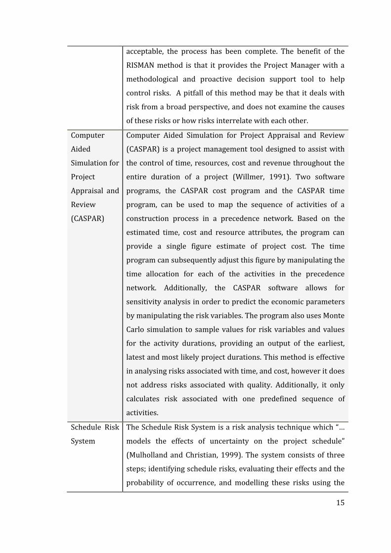
Table 2.1: Risk Analysis Methods

METHOD OVERVIEW

RISMAN Risk

Management

Method

In the Netherlands, the RISMAN risk management method has

been widely adopted as a tool to analyse, quantify and manage

risks associated with large infrastructure construction projects.

The following diagram illustrates the six step process of the

RISMAN method (Soares, 1997).

Determination of purpose

Identification of uncertanties

Quantification of uncertainties

Calculation of project risk

Identification and quantification measures

Calculation of effectiveness of measures

Result acceptable?Completion of RISMAN

methodYes

No

Figure 2.1: The RISMAN method (Soares, 1997).

Determination of purpose involves determining the focus,

whether it be time, quality, or cost related. Secondly the

uncertainties must be identified and grouped into three

categories; normal (due to stochastic nature of reality), special

(very low probability of occurrence but high impact), and plan

uncertainties (uncertainties at initial stages of project).

Uncertainties are then quantified and are used to calculate the

level of project risk by means of Monte Carlo simulation. The

Project Manager must then assess the risks if necessary given

some of them may have changed over time, and new risks may

have been identified. Once the results have been deemed

15

acceptable, the process has been complete. The benefit of the

RISMAN method is that it provides the Project Manager with a

methodological and proactive decision support tool to help

control risks. A pitfall of this method may be that it deals with

risk from a broad perspective, and does not examine the causes

of these risks or how risks interrelate with each other.

Computer

Aided

Simulation for

Project

Appraisal and

Review

(CASPAR)

Computer Aided Simulation for Project Appraisal and Review

(CASPAR) is a project management tool designed to assist with

the control of time, resources, cost and revenue throughout the

entire duration of a project (Willmer, 1991). Two software

programs, the CASPAR cost program and the CASPAR time

program, can be used to map the sequence of activities of a

construction process in a precedence network. Based on the

estimated time, cost and resource attributes, the program can

provide a single figure estimate of project cost. The time

program can subsequently adjust this figure by manipulating the

time allocation for each of the activities in the precedence

network. Additionally, the CASPAR software allows for

sensitivity analysis in order to predict the economic parameters

by manipulating the risk variables. The program also uses Monte

Carlo simulation to sample values for risk variables and values

for the activity durations, providing an output of the earliest,

latest and most likely project durations. This method is effective

in analysing risks associated with time, and cost, however it does

not address risks associated with quality. Additionally, it only

calculates risk associated with one predefined sequence of

activities.

Schedule Risk

System

The Schedule Risk System is a risk analysis technique which “…

models the effects of uncertainty on the project schedule”

(Mulholland and Christian, 1999). The system consists of three

steps; identifying schedule risks, evaluating their effects and the

probability of occurrence, and modelling these risks using the

16

Program Evaluation and Review (PERT) statistical technique to

determine the project’s schedule risk profile. What is interesting

about this approach is its introduction of a knowledge

management program called HyperCard. HyperCard essentially

serves as a database of schedule risks which are stored and

transferred in every project, to be used at the schedule risk

identification stage. The downside of this technique, however, is

that it focuses solely on time and can only be used to assess

project schedule risk.

Judgmental

Risk Analysis

Process—

JRAP

Judgemental Risk Analysis Process (JRAP) is a schedule risk

analysis method. It has been defined as, ”… a pessimistic risk

analysis methodology or a hypothesis based on Monte Carlo

simulation that is effective in uncertain conditions due to its

capability of converting uncertainty to risk judgmentally in

construction projects”. (Oztas and Okmen, 2004). The first phase

of JRAP is ‘risk identification’, wherein the risks which can affect

time are brainstormed. Following this is the ‘risk measurement’

phase, where the probability of these risks occurring, and their

estimated impact on the project schedule are evaluated and

quantified. The method then uses Monte Carlo simulation to

observe the variations in activity durations based on the input of

the first two steps. The output of this method provides insight

into the likely project duration, the most critical activities, and

which risk elements have the greatest effect on project duration.

This method, however, does not assess risks associated with cost

and quality.

Estimating

Project and

Activity

Duration

Using

Network

More realistically predicting a construction project’s duration

requires a methodology which considers the dependency

between the activities. A risk management approach has been

proposed which uses historical data to associate risk factors

with the activities which form the construction schedule. Once

the activity durations have been estimated, the risks can be

17

Analysis analysed using probability distribution for project duration

forecasts, as well as to determine the individual effects of risk

factors on the project schedule (Dawood, 1998). This method

essentially provides the same output as the JRAP method, and

similarly has the same shortcoming of only analysing risk

associated with time.

Data-Driven

Analysis of

Corporate

Risk Using

Historical

Cost-Control

The article, ‘Data-Driven Analysis of Corporate Risk Using

Historical Cost-Control’, makes a distinction between local and

“corporate” approaches to dealing with risk (Minato and Ashley,

1998). The first, local method is one which is more traditionally

adhered to, wherein the individual risks are analysed upon their

own merit. The corporate approach, however, groups ‘corporate

risks’ according to similarity, to ensure that organisations

overlooking a portfolio of projects are not overwhelmed by the

vast amount of risks which could affect each of their projects.

The following equation expresses the total risk of a project

according to the authors:

Total risk = Dependent Risk + Independent Risk

Independent risk involves risks which are unique to a project

and will not affect other projects within the portfolio, while

dependent, corporate risks are those which arise “…due to

interactions of common risk factors among multiple projects”

(Minato and Ashley, 1998). Regression statistics are then applied

to historical cost data to assess the cost impact of these

dependent risks. This methodology is unique and is an effective

means of assessing cost performance. It does not, however,

consider risks associated with time and quality. Additionally,

because corporate risks will vary based on the organisational

structure of different contractors, this approach would require

extensive data analyses to be performed for every organisation

18

looking to adopt it. Consequently, its ability to be universally

adopted is questionable.

Estimating

Using Risk

Analysis—

ERA

Estimating using Risk Analysis (ERA) has been propagated as an

effective tool for calculating the financial implications of risk for

the objective of determining project contingencies (Mak and

Picken, 2000). The methodology behind this tool consists first of

estimating the base cost of a construction project, with disregard

to any possible risks. Then, the project team must identify a list

of fixed and variable risks. Fixed risks are those which either

occur with complete effect, or do not occur at all. Variable risks,

however, are those which have varying degrees of impact on

cost. The team must then calculate the average risk allowance

and maximum risk allowance for each risk using predefined

formulas. An average of these two outputs is then calculated to

produce the average risk estimate, and the maximum likely

estimate. Although this is an effective method for assessing risks

associated with cost for the preparation of tender packages, its

shortcoming is its disregard for both time and quality (Imbeah,

2007).

Failure Modes

and Effects

Analysis—

FMEA

Failure Modes and Effects Analysis (FMEA) is a risk assessment

tool adopted by the construction industry for the purpose of

identifying all possible, potential project failures (Talon et al.,

2008). Essentially, failures are assessed according to

characteristics such as the cause of failure, and the consequence

of its occurrence. Following this, a scale of 0-10 is used to

subjectively evaluate “… the likelihood of occurrence of the

phenomena, the level of significance related to the consequence

of failure of the component and, the degree of detectability of

failure” (Talon et al., 2008). This evaluation provides an

organisation with insight into the nature of its failures, and can

subsequently be used to prevent or minimise the effect of future

failure events. Furthermore, FMEA takes into account the

19

consequence of a failure in terms of its effect on all three major

facets of project management; time, cost and quality, and

therefor provides for a well-rounded risk assessment tool.

Program

Evaluation

and Review

Technique—

PERT

The Program Evaluation and Review Technique (PERT) is

essentially a project management tool for assessing risk

associated with time in projected schedules (Malcolm et al.,

1959). For each activity that forms part of the construction

process, three variables must be given; the optimistic, most

likely, and pessimistic estimates of duration. Additionally, flow

diagram must be formed which visually represents the

dependencies and sequence of activities. Based on this input, the

mean duration and variance of each activity can be calculated.

PERT provides Project Managers with a means of assessing the

risks associated with time, and the different ways in which

delayed activity durations can affect the project schedule as a

whole (Roman, 1962). While PERT provides an effective means

of assessing the risk of activity delays, it does little to take into

account risks associated with cost and quality.

Monte Carlo

Process

Monte Carlo analysis is a stochastic simulation method which

can determine the probability of a project’s outcome by running

a number of iterations; the accuracy of the output enhanced by

the number of the iterations. The accuracy is also dependent on

the subjective input that is required before the simulation can be

performed. These inputs include quantification of probability

occurrence and probability distribution of the risk factors

(Akintoye and MacLoed, 1997). The advantage of Monte Carlo

analysis is that it can be used to estimate the project cost based

on a probable cost distribution, as well as the project duration

based on the input of a probable time distribution. Because the

accuracy of the output is based solely on the integrity of the

input data, this risk analysis method is only suitable should a

proficient data collection methodology be in place.

20

Advanced

Programmatic

Risk Analysis

and

Management

Model

(APRAM)

Imbeah and Guikema (2009) propose the Advanced

Programmatic Risk Analysis and Management Model (APRAM)

as a solution to managing risk in construction projects (Imbeah

and Guikema, 2009). The model, developed for the aerospace

industry, essentially comprises of the following steps;

determining the total budget, identification of possible system

configurations, determination of the residual budget

(formulated by determining difference between total project

estimate and cost of configuration), identification of technical

failures and managerial problems, optimization and

determination of technical reinforcement budget, optimization

and determination of best response to managerial problems, and

selection of the optimal alternative and allocation of residual

budget that minimises overall failure risk. Identification of

failure modes and assigning probabilities is to be performed “…

based on expert elicitation of probabilities with the project

management team using established elicitation methods”

(Imbeah and Guikema, 2009). APRAM provides mathematical

expressions for calculating the cost of failure, and offers

solutions to lowering these costs through optimisation of the

residual budget. A limitation of this method, however, is its

dependency on the project team to subjectively determine the

probability of failures. Additionally, because APRAM analyses

risk on the scale of material type used, applying the methodology

to large projects may prove overly complex and time consuming.

DISCUSSION

The risk analysis methods discussed all provide alternative means of assessing

risk in construction. Their applicability and effectiveness depends entirely on the

specific nature of the project and the types of risks that need to be analysed. Of

the methods analysed, only two provide as a tool for measuring risks of all three

project management constraints; time, cost and quality.

21

The first of these tools is the Failure Modes and Effects Analysis (FMEA)

technique. When conducting an FMEA, the cause, effect, and probability of

failures are analysed. Additionally, for each failure mode, preventative measures

can be recommended in order to prevent their occurrence. This tool does not,

however, take into the consideration of risk interrelationship; how one risk’s

probability may be influenced by project specific factors. The second tool which

assesses time, cost and quality, is the Advanced Programmatic Risk Analysis and

Management Model (APRAM). The strength of APRAM is its comprehensiveness

in assessing the risks on a very small scale; beginning with the types of materials

used. This attention to detail, however, is also its pitfall. Larger projects with a

wider spectrum of components and materials will inherently involve an

exponentially larger amount of risks; an amount which could perhaps be too

many to individually assess for every new project. Additionally, relying on the

subjective assessment of failure probabilities from the project team at hand for

risks associated with material failure and such is not practical. A more valid

approach to data collection would be seeking professional advice from those who

are most familiar with the failures.

In assessing the risk of occupational hazards in the construction industry, Liu and

Tsai (2012) establish that current approaches to risk assessment can broadly be

categorised into the following groups; qualitative analysis (checklists,

interviews), semi-quantitative analysis (matrix method, FMEA), and quantitative

analysis (decision tree analysis, sensitivity analysis). Qualitative analysis is the

most popular given the accessibility of the data. The subjective nature of this

method, however, weakens the integrity of its output. While quantitative analysis

provides the most objectively accurate output, obtaining objective data relating

to the cause and effect relationships of risk failures is difficult (Liu and Tsai,

2012).

Consequently, the most practical means of assessing risk in construction is

through the application of a semi-quantitative analysis. This involves formulating

an approach which uses both qualitative and quantitative assessment methods.

Similarly to FMEA, a qualitative means of data collection should be performed,

22

using expert opinion about the sources of failure, the impact of these failures, and

their underlying mechanisms.

In order to assess qualitative data through means of a quantitative assessment

method, Mahant (2004) proposes the use of fuzzy logic.

“Fuzzy logic and fuzzy set operations enable characterization of vaguely

defined (or fuzzy) sets of likelihood and consequence severity and the

mathematics to combine them using expert knowledge, to determine risk”.

- (Mahant, 2004).

The output of these fuzzy logic operations could then be used as input for a

quantitative analysis, such as Monte Carlo simulation. Based on the assessment of

the risk analysis methods identified (See Table 2.1), it is apparent that the

construction industry lacks a semi-quantitative risk analysis method which can

effectively and practically assess risks associated with time, cost and quality.

Accordingly, the following methodology will explain a model which can perform

this task with the objective of assessing failure cost and their risks in

geotechnical construction projects.

23

3.0 RESEARCH METHODOLOGY

Based on the literature review, the following model has been developed which

simulates the potential risk of failure associated with the building pit

construction process, and generates cost profiles for multiple construction

sequences, inclusive of risk and resultant failure costs. The model draws upon

the concept that failure costs emanate from two sources; local failure risks and

global failure risks (Hegazy et al., 2011). The model comprises of the following

seven stages:

1. Define the activities and methods which are involved in the building pit

construction process. The model could easily be applied to another

construction process by instead defining the activities and methods

specific to that process.

2. Define the parameters of the project and process. This involves all of the

unique characteristics and risks inherent to project and the methods

which comprise its process.

3. Based on the defined activities, methods, and parameters, generate all of

the plausible sequences of construction.

4. Estimate the base costs for each construction sequence based on the

production and cost unit rates.

5. In preparation for the Monte Carlo Simulation, assign the assumption

input variables.

6. Perform Monte Carlo Simulation for each method within each

construction sequence.

7. Analyse the output of the simulations.

The following diagram depicts the seven stages of the proposed model, followed

by the research methodology. The research methodology is structured as such

that it will systematically describe how the data was collected and applied at

each of the seven stages of the model. The following chapter (See Section 4.0)

demonstrates how the model can be applied in practice.

24

Define projectParameters

(e.g. pit depth)

Interrelationship between project and process parameters

Define processParameters

(e.g. vibration noise)

Interrelationship between process

and risk parameters

Define riskParameters

(e.g. local failure risk)

Define activities & methods

Stage 1

Stage 2

Stage 3

Generate sequences

Stage 4

Calculate costs

Stage 5

Assign assumption inputs

Stage 6

Monte Carlo Simulation

Stage 7

Analysis of Results

Figure 3.1: Seven stages of the model

3.1 STAGE 1: DEFINE ACTIVITIES & METHODS

A survey research was performed in order to obtain qualitative data for the

development of the model. Six experts within the industry were approached for

interviews and questionnaires relating to; the methods and activities inherent to

the building pit construction process, the sources of failures, and the underlying

mechanisms of failure sources.

25

In order to determine what risks are involved, first the nature of the building pit

construction process had to be analysed. Based on the interviews, the following

was concluded.

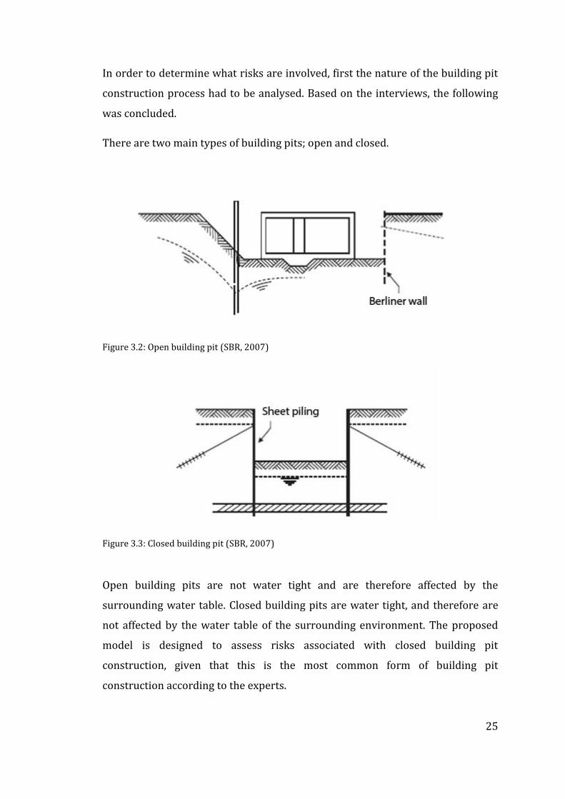
There are two main types of building pits; open and closed.

Figure 3.2: Open building pit (SBR, 2007)

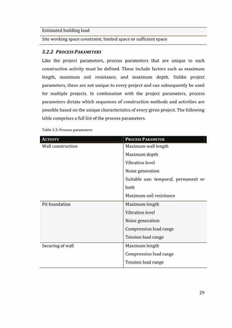
Figure 3.3: Closed building pit (SBR, 2007)

Open building pits are not water tight and are therefore affected by the

surrounding water table. Closed building pits are water tight, and therefore are

not affected by the water table of the surrounding environment. The proposed

model is designed to assess risks associated with closed building pit

construction, given that this is the most common form of building pit

construction according to the experts.

26

Closed building pit construction comprises of the following activities and

methods:

Table 3.1: Close building pit construction methods

ACTIVITY POSSIBLE AVAILABLE METHOD

Wall construction Berliner wall, driven

Concrete retaining wall, driven

Steel retaining wall (sheet piling), driven

Combi-wall, driven

Deep wall (diaphragm)

Bored-pile wall

Excavation Dry Excavation

Wet Excavation

Pit bottom sealing

(waterproofing)

Artificial sealing with concrete

Artificial sealing with underwater concrete

Pit foundation Concrete pre-fabricated piles

Hollowed steel piles

Linked concrete piles

Hollow concrete pipes

Tube segments piles

MV-Piles

Securing of wall Strut – steel pipe

Anchor

Dewatering Source pumping

The following tree-diagram illustrates the activities and methods involved in

closed building pit construction projects.

27

Wall construction ExcavationPit bottom sealing

(waterproofing)Pit foundation Securing of wall Dewatering

Berliner wall, driven

Concrete retaining wall

Steel retaining wall

Combi-wall, driven

Deep wall (diaphragm)

Bored-pile wall

Dry

Wet

Artificial sealing (concrete)

Artificial sealing (underwater

concrete)

Concrete prefabricated pile

Hollowed steel pipe

Linked concrete piles

Hollow concrete

pipes

Tube segments piles

MV-Piles

Strut – steel pipe

Anchor

Source pumping

Legend

Activity

Method

Figure 3.4: Close building pit methods and activities

28

3.2 STAGE 2: DEFINE PARAMETERS

The parameters essentially describe that nature of the project, the nature of the

risks involved, and the limitations of the construction methods available. By

defining these parameters, plausible sequences of construction and their

inherent risks can be determined. The project, process, and risk-related

parameters, as well as how they interrelate will now be described.

3.2.1 PROJECT PARAMETERS

Project parameters are essentially the characteristics unique to a particular

construction project. Only when the project parameters are defined can suitable

construction methods be selected. The reason for this is that certain construction

methods are only suitable in certain scenarios. For example, a particular method

of wall construction may not be suitable given that the project has a pit depth of

over five metres.

The following parameters were decided upon based on discussion with experts.

Table 3.2: Project parameters

PROJECT PARAMETER

Pit wall parameter

Pit depth

Pit area

Wall maximum length

Acceptable vibration level

Acceptable noise level

Soil resistance; hard layer, medium layer, or soft layer

Soil classification; Sand, clay, or peat

Impermeable layer; present or not

Ground level reference

Ground water level

Surrounding environment

Construction type; permanent or temporal

29

Estimated building load

Site working space constraint; limited space or sufficient space

3.2.2 PROCESS PARAMETERS

Like the project parameters, process parameters that are unique to each

construction activity must be defined. These include factors such as maximum

length, maximum soil resistance, and maximum depth. Unlike project

parameters, these are not unique to every project and can subsequently be used

for multiple projects. In combination with the project parameters, process

parameters dictate which sequences of construction methods and activities are

possible based on the unique characteristics of every given project. The following

table comprises a full list of the process parameters.

Table 3.3: Process parameters

ACTIVITY PROCESS PARAMETER

Wall construction Maximum wall length

Maximum depth

Vibration level

Noise generation

Suitable use: temporal, permanent or

both

Maximum soil resistance

Pit foundation Maximum length

Vibration level

Noise generation

Compression load range

Tension load range

Securing of wall Maximum length

Compression load range

Tension load range

30

Additionally, at this stage the production and cost unit rates of the construction

methods also form part of the process parameters. This ensures that time, cost,

and quality for each sequence can be estimated. A full list of production and cost

unit rates has been composed (See Section 8.1). It should be noted that the cost

rates for each of the activities should be updated to reflect current prices.

Additional remarks which could potentially affect the cost of the activities were

also stored in a table (See Section 8.2).

3.2.3 INTERRELATIONSHIP BETWEEN PROJECT AND PROCESS PARAMETERS

The interrelationships between project and process parameters are used to filter

plausible methods of construction. For example, a process parameter for the

‘Berliner wall’ construction method is that the maximum retention depth is 6m. If

the project has a parameter of a retention depth being greater than 6m, then the

‘Berliner wall’ construction method will be excluded from the next phase of the

model, sequence generation.

3.2.4 RISK PARAMETERS

The risk parameters of building pit construction essentially comprise of the

sources of local and global failure risks, the underlying mechanisms of these

failure sources, the local and global failure risks, as well as their impact on time

and cost.

SOURCES OF FAILURE

Industry experts were asked to state which they considered to be the most

common sources of failure. This knowledge elicitation process was facilitated by

a semi-structured interview protocol based on the following questions.

How would you define failure costs in construction?

Based on your experience in the Dutch construction industry, what are

the main sources of failure costs in construction projects?

Can you put these failure costs in order of their likelihood of

occurrence?

Can you differentiate between failure costs in terms of being product-

related or process related?

31

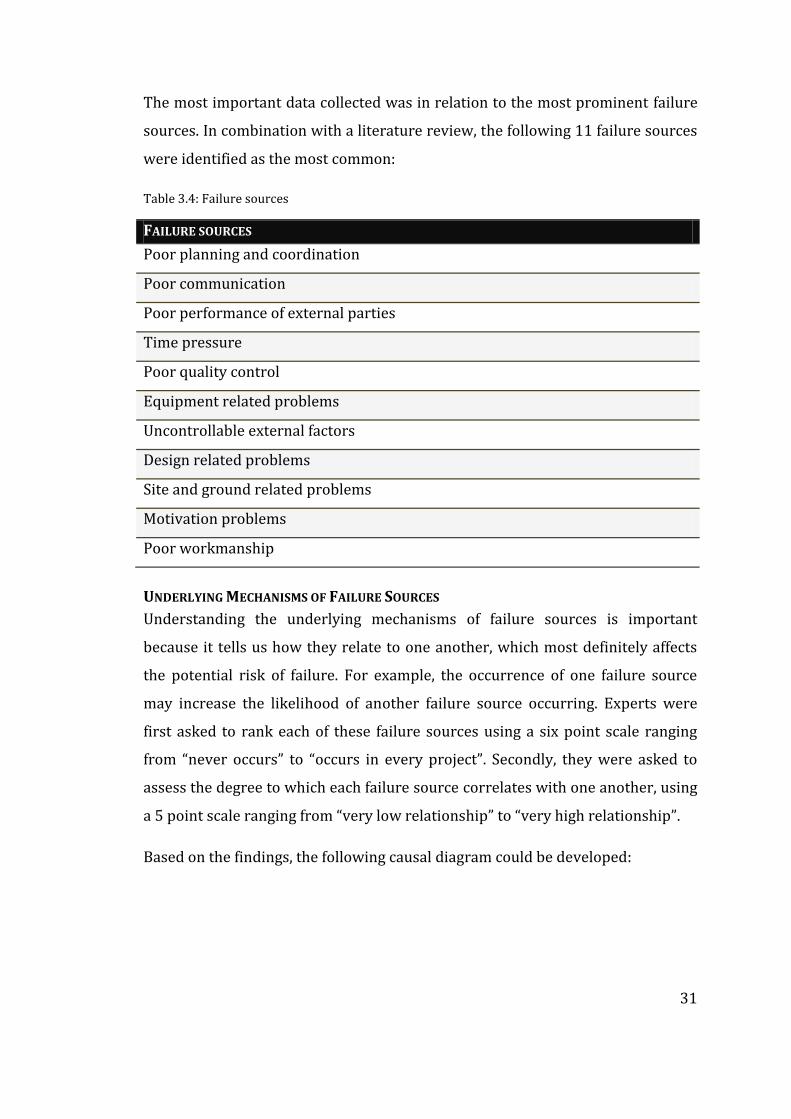
The most important data collected was in relation to the most prominent failure

sources. In combination with a literature review, the following 11 failure sources

were identified as the most common:

Table 3.4: Failure sources

FAILURE SOURCES

Poor planning and coordination

Poor communication

Poor performance of external parties

Time pressure

Poor quality control

Equipment related problems

Uncontrollable external factors

Design related problems

Site and ground related problems

Motivation problems

Poor workmanship

UNDERLYING MECHANISMS OF FAILURE SOURCES

Understanding the underlying mechanisms of failure sources is important

because it tells us how they relate to one another, which most definitely affects

the potential risk of failure. For example, the occurrence of one failure source

may increase the likelihood of another failure source occurring. Experts were

first asked to rank each of these failure sources using a six point scale ranging

from “never occurs” to “occurs in every project”. Secondly, they were asked to

assess the degree to which each failure source correlates with one another, using

a 5 point scale ranging from “very low relationship” to “very high relationship”.

Based on the findings, the following causal diagram could be developed:

32

LegendPPC: Poor planning and coordinationCOM: Poor communicationPPE: Poor performance of external partiesTPR: Time pressurePQC: Poor quality controlEQP: Equipment related problemUEF: Uncontrollable external factorsDRP: Design related problemsSGR: Site and ground related prblemsMOT: Motivation problemsPWK: Poor workmanship

Figure 3.5: Underlying mechanisms of failure sources (Castillo et al., 2009)

LOCAL FAILURES

Having identified the activities and methods, and sources of failure inherent to

building pit construction, experts were asked to identify their local and global

risks. Local risks are those which affect only the activity where the failure occurs,

whereas global risks are those which, when having occurred, affect the process as

a whole. The following table lists some of the local failure risks inherent to the

different building pit construction activities. A full list of failure risks has also

been composed (Refer to Appendix 8.3).

Table 3.5: Local failures

LOCAL FAILURES

Sheet pile is not at the correct depth

Sheet pile is out of the lock

Damage to the sheet pile

Insufficient waterproofing of wall

Cement bentonite wall not cured

Pile wall not at the correct depth

Slot instability

Instability of pile wall section

33

Overconsumption concrete

Different element size

Abnormal strength element

Do not arrive at depth element

GLOBAL FAILURES

The following global failure risks were then identified:

Table 3.6: Global failures

GLOBAL FAILURES SHORT DESCRIPTION

Damage to foundations

due to excavation

If excavation is carried out after laying foundations, it

is likely to damage the head of the foundation

elements

Deformation of wall due

to excavation

If excavation is dry it is likely to triggered a wall

deformation because of horizontal load unbalance.

Deformation of the wall

due to excavation and

dewatering

If excavation is wet then during dewatering of pit it is

likely to trigger a wall deformation because of

horizontal load unbalance.

Settlement in the

surroundings due to

vibration during wall

construction

If wall construction method generates vibration it is

likely to trigger a settlement in the surroundings.

Settlement in the

surroundings due to

deformation of the wall

If deformation of the wall occurs, it is very likely to

cause damage to the surroundings.

For both the local and global failure risks, experts were asked to give a

percentage score (with 5% intervals) as to what they perceived the average

probability of occurrence being.

METHOD SPECIFIC RISK

Experts were asked to state which methods were more prone to certain local or

global failure risks. For example, the ‘instability of pile wall section’ local failure

34

risk may have a higher chance of occurring should a certain type of construction

method be used. Based on these results, the multiplying factors were assigned to

construction methods to increase the probability of failure for certain failure

events.

IMPACT ON TIME & COST

Additionally, experts were asked to rank the impact on both time and cost for

each of the failure risks should they occur, using a Likert scale from one (very

low impact) to two (very high impact).

1 2 3 4 5

Very

low

impa

ct

Low

impa

ct

Aver

age

impa

ct

Hig

h im

pact

Very

hig

h im

pact

Figure 3.6: Likert scale assessing impact on time and cost

When collecting data related to the impact on cost, experts were shown the

following cost-range matrix (See table 3.7). This ensured that realistic figures

were given and that answers from the various respondents correlated. A more

realistic approach, however, would be to ascertain estimates of the impact on

cost from professional cost estimators. Given time limitations, however, this was

not feasible. For the purpose of explaining the functioning of the proposed model,

it was also not necessary.

Table 3.7: Cost range matrix for impact on cost.

Impact on cost 1 2 3 4 5

Cost range 1000 2000 25,000 100,000 250,000

35

3.2.5 INTERRELATIONSHIP BETWEEN PROCESS AND RISK PARAMETERS

A correlation must then be drawn between the process and risk parameters. This

involves drawing a link between the process dependencies of failure sources, as

well as the failure sources and failure risks.

PROCESS DEPENDENCIES OF FAILURE SOURCES

Once the failure sources had been identified, experts were asked to draw a link

between the occurrence of one failure source and its influence on another.

Because failures are often linked to each other, incorporating these relationships

into failure cost calculation will yield more realistic results. This information was

stored in a matrix for future use.

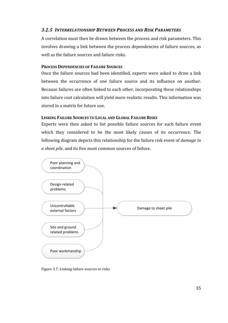
LINKING FAILURE SOURCES TO LOCAL AND GLOBAL FAILURE RISKS

Experts were then asked to list possible failure sources for each failure event

which they considered to be the most likely causes of its occurrence. The

following diagram depicts this relationship for the failure risk event of damage to

a sheet pile, and its five most common sources of failure.

Poor planning and coordination

Design related problems

Uncontrollable external factors

Site and ground related problems

Poor workmanship

Damage to sheet pile

Figure 3.7: Linking failure sources to risks

36

3.2.6 DATA ANALYSIS

The following is a summary of the risk-related data that was obtained throughout

the data collection process:

Table 3.8: Risk-related data

DATA DATA COLLECTION METHOD

Local and global risk

failure probability

For each of the risks, experts were asked to give a

percentage score (with 5% intervals) as to what they

perceive the average probability of occurrence being.

Impact on cost of

failure events

Experts were asked to use a Likert scale ranging from 1

(very low) to 5 (very high) to assess the impact on cost for

each of the failure events.

Impact on time of

failure events

The same Likert scale was used for the assessment of

impact on time for each of the failure events.

Failure sources For each failure event, experts were asked to assign

failure sources which they believe most heavily influence

that event occurring. Once these three factors had been

established, they were then asked to provide a subjective

correlation value between the factor and the failure event.

The following section will now describe how some of this data was analysed to

ensure applicability with the model.

KENDALL’S COEFFICIENT

Kendall’s Coefficient of Concordance was used in order to determine the extent of

agreement between the interviewees in relation to their assessment of failure

sources. The coefficient provides a nonparametric measure of concordance and is

calculated using the following formula:

37

Legendm = number of groupsn = number of objectsR = overall rank given to variableT = tied correlation value

Figure 3.8: Kendall’s coefficient formula (Siegel and John Castellan, 1988).

The number of groups in this case is three, given general contractors,

consultants, and clients were interviewed. The number of objects is 11, given 11

failure sources were identified. The overall rank given to the variable, the failure

source, is a range from 1 to 12, ascending from most frequent occurrence to least.

The tied correctional value provides a correction for the effect of repeating, or

tied, ranks within a data set, and can be calculated with the following formula:

Legendt = number of tied ranksg = number of groups

Figure 3.9: Tied correctional value (Siegel and John Castellan, 1988).

Based on this analysis, a more balanced perspective of the most common sources

of failure could be depicted. This formed as a framework for determining the

underlying mechanisms of failure sources (Refer to 3.2.2).

FUZZY LOGIC

Once the failure risks had been collected, it was important to grasp that these

risks would be affected by the project parameters (Refer to 3.2.2) inherent to the

individual project at hand. Estimating risk values for highly specific scenarios,

however, is not practical and likely to yield inaccurate results.

Fuzzy logic methodology “…provides a way to characterize the imprecisely

defined variables, define relationships between variables based on expert human

knowledge and use them to compute results” (Mahant, 2004). By defining value

38

sets, such as low (0-40%), medium (30-70%), and high probability (70-100%),

multiple scenarios can be assessed and categorised into one of these groups.

For example, soil resistance has been classified into three groups; hard layer (1),

medium layer (2), and soft layer (3). Using fuzzy logic methodology, the following

framework could be formulated for the failure event of damage to sheet pile, and

the construction method of steel retaining wall (sheet piling).

Table 3.9: Use of fuzzy logic

SCENARIO IMPACT ON FAILURE RISK

IF soil resistance IS hard 3

IF soil resistance IS medium 2

IF soil resistance IS soft 1

What this logic states is that the risk of damage to sheet pile, as defined in the

data collection stage, will be influenced by a factor of 1, 2 or 3, dependent on the

nature of the soil. Fuzzy logic was used for multiple scenarios for a number of

different construction methods and risks, and is important because it allows for

more accurate predictions

3.3 STAGE 3: GENERATE SEQUENCES

In order to understand what risks are involved in a construction process, it is

important to first determine its inherent sequence of activities. Discussion with

experts led to a conclusion that only three sequences of activities were plausible.

These sequences could be derived by posing the following two questions:

- Is there a natural impermeable layer below the pit which can be used to

seal the pit bottom?

- What type of excavation method will be selected?

The following flow chart represents this derivation process;

39

Is there a natural impermeable layer below the pit which can be used to seal the pit

bottom?

Basic sequence is:1. Wall construction2. Securing of wall3. Pit foundation4. De-watering of pit5. Excavation (dry)6. Pit bottom sealing

No

Wet

Dry

Yes

What type of excavation method will be selected?

Basic sequence is:1. Wall construction2. Securing of wall3. Pit foundation4. Pit bottom sealing5. De-watering of pit6. Excavation (dry)

Basic sequence is:1. Wall construction2. Securing of wall3. Excavation (wet)4. Pit foundation5. Pit bottom sealing6. De-watering of pit

Figure 3.10 Sequence generation based on two closed-questions

The sequence generation phase is dependent upon data input from the

‘interrelationship between project and process parameters’ stage. Ultimately,

there are three fundamental activity sequences of the building pit construction

process (See Figure 3.10). The following table depicts these three scenarios.

40

Table 3.10: three potential closed building pit sequences

SEQUENCE 1 SEQUENCE 2 SEQUENCE 3

1. Wall construction

2. Securing of wall

3. Pit foundation

4. De-watering of pit

5. Excavation (dry)

6. Pit bottom sealing

1. Wall construction

2. Securing of wall

3. Pit foundation

4. Pit bottom sealing

5. De-watering of pit

6. Excavation (dry)

1. Wall construction

2. Securing of wall

3. Excavation (wet)

4. Pit foundation

5. Pit bottom sealing

6. De-watering of pit

The sequence of activities are to be manually selected by the Project Manager

based on the conditions of the site, and whether dry or wet excavation is more

suitable (See Figure 3.10). The following network diagram displays all possible

sequences of methods possible for the construction of the building pit for

sequence 1 of activities.

41

Wall construction ExcavationPit bottom sealing

(waterproofing)Pit foundationSecuring of wall Dewatering

Berliner wall, driven

Concrete retaining wall

Steel retaining wall

Combi-wall, driven

Deep wall (diaphragm)

Bored-pile wall

Dry

Wet

Artificial sealing (concrete)

Artificial sealing (underwater

concrete)

Concrete prefabricated pile

Hollowed steel pipe

Concrete hollowed pipe

Ask saad

Ask saad

Ask saad

Strut – steel pipe

Anchor

Source pumping

Met

ho

ds

Act

ivit

ies

Figure 3.11: Network diagram of construction methods

42

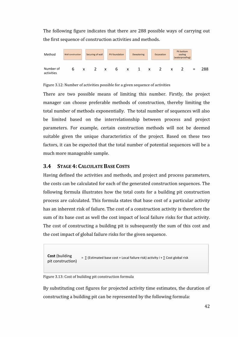
The following figure indicates that there are 288 possible ways of carrying out

the first sequence of construction activities and methods.

Wall construction ExcavationPit bottom

sealing (waterproofing)

Pit foundationSecuring of wall DewateringMethod

Number ofactivities

x x x x x =6 2 6 1 2 2 288

Figure 3.12: Number of activities possible for a given sequence of activities

There are two possible means of limiting this number. Firstly, the project

manager can choose preferable methods of construction, thereby limiting the

total number of methods exponentially. The total number of sequences will also

be limited based on the interrelationship between process and project

parameters. For example, certain construction methods will not be deemed

suitable given the unique characteristics of the project. Based on these two

factors, it can be expected that the total number of potential sequences will be a

much more manageable sample.

3.4 STAGE 4: CALCULATE BASE COSTS

Having defined the activities and methods, and project and process parameters,

the costs can be calculated for each of the generated construction sequences. The

following formula illustrates how the total costs for a building pit construction

process are calculated. This formula states that base cost of a particular activity

has an inherent risk of failure. The cost of a construction activity is therefore the

sum of its base cost as well the cost impact of local failure risks for that activity.

The cost of constructing a building pit is subsequently the sum of this cost and

the cost impact of global failure risks for the given sequence.

= ∑ (Estimated base cost + Local failure risk) activity i + ∑ Cost global riskCost (building pit construction)

Figure 3.13: Cost of building pit construction formula

By substituting cost figures for projected activity time estimates, the duration of

constructing a building pit can be represented by the following formula:

43

= ∑ (Estimated duration + Local failure risk) activity i critical path + ∑ Time global riskTime (building pit construction)

Figure 3.14: Duration of building pit construction formula

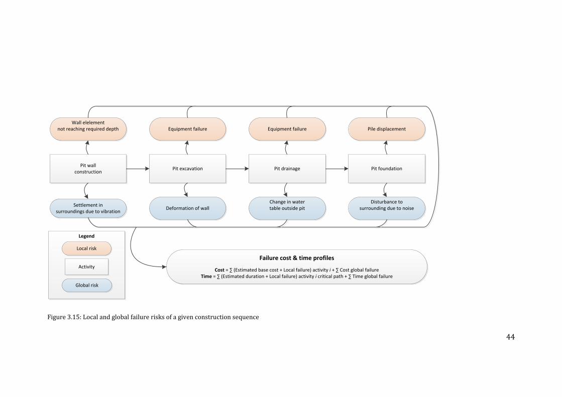
The following diagram depicts how each activity has local and global failure risks

which affect the output of the proposed model:

44

Legend

Pit wall construction

Pit excavation Pit drainage Pit foundation

Settlement insurroundings due to vibration

Deformation of wallChange in watertable outside pit

Disturbance to surrounding due to noise

Wall elelement not reaching required depth Equipment failure Equipment failure Pile displacement

Local risk

Activity

Global risk

Failure cost & time profiles

Cost = ∑ (Estimated base cost + Local failure) activity i + ∑ Cost global failure Time = ∑ (Estimated duration + Local failure) activity i critical path + ∑ Time global failure

Figure 3.15: Local and global failure risks of a given construction sequence

45

The formula involves the calculation of base costs and failure costs. In this model,

failure costs are determined in the following stage using Monte Carlo simulation.

Therefore, at this stage only the base costs must be calculated.

The base costs are simply an estimation of the project costs, based on the

methods comprising the construction sequence. The base costs are estimated

traditionally incorporating material, labour and plan. See Section 8.1 for a list of

production and unit cost rates used in this model. The following section will

describe how assumption inputs are assigned to incorporate failure costs to

determine the total cost of building pit construction.

3.5 STAGE 5: ASSIGN ASSUMPTION INPUT

In this model, Monte Carlo simulation is used to generate a cost profile for each of

the identified construction sequences. As explained in the literature review, the

Monte Carlo simulation method uses the quantification of probability occurrence

and probability distribution of the risk factors to determine the probability of a

project’s outcome by running a series of iterations; the accuracy thereby

increasing with the number of simulations (Akintoye and MacLoed, 1997).

To define a normal probability distribution, three inputs are required; a most

likely value, and a lower (1st parameter) and higher (2nd parameter) value. These

values define the variation range wherein the simulation will select a result. The

following figure displays this graphically.

46

Figure 3.16: Normal distribution graph.

The following table describes how assumption inputs are assigned using data

collected for this model.

Table 3.11: Assumption input for use in model

ASSUMPTION INPUT DESCRIPTION

Most likely The most likely value of the normal distribution is the

estimated base cost of the construction method. This is

can be calculated using given production and cost unit

rates (See Section 8.1)

1st Parameter Based on expert advice, the 1st parameter should be 0.9

times the base cost of the construction method.

2nd Parameter Based on expert advice, the 2nd parameter should be 1.1

times the base cost of the construction method.

Because a construction method maybe susceptible to the risk of a failure

occurring, this must be incorporated when defining assumptions. Should a failure

47

event occur, it is the second parameter which will be affected. To adjust the value

of input for the second parameter, we must incorporate a risk factor.

RISK OF FAILURE

Risk can be defined as “the product of probability of the hazard and its potential

impact”, as illustrated in the following diagram (CEEP, n.d.).

= Probability X ImpactRisk

Figure 3.17: Risk formula.

The impact on cost and probability of occurrence can then be used to determine

the failure cost risk for each construction method. This risk factor can be added

to the 2nd parameter to increase the range, ensuring that the distribution is

susceptible to the risk of failure costs. Table 3.7 demonstrates how the impact on

cost for each failure is determined. The following section will explain how the

probability of failure is calculated.

PROBABILITY OF FAILURE

To determine the risk of a failure event, both the probability of its occurrence, as

well as its impact on cost are required. The probability of a failure event

occurring, however, is dependent on four factors; the failure risk, the failure

sources, the method-specific risk, and process dependencies. This ensures that

the probability of failure is adjusted based on the specificities of the project at

hand. The following example scenario demonstrates how the impact on cost and

probability of risk failures are used to incorporate risk as input for the Monte

Carlo simulations.

EXAMPLE SCENARIO

The following example will demonstrate how the inputs would be assigned based

on the characteristics of a given construction method. The details of the method

are as follows.

48

Table 3.12: Example scenario of Method & associated risks

BASE COST RISK 1 RISK 2

€10,000 Impact on cost

€20,000

Impact on cost

€2,000

Probability

0.02

Probability

0.34

Risk = €400 €680

For this example we can determine the following:

Base cost = €10,000

1st Parameter = €10,000 x 0.9 = €9,000

2nd Parameter = (€10,000 x 1.1) + Risk factor

Given we have two risk factors, it is important to select the largest risk factor to

ensure that all failure cost risks are accounted for. In this example risk two has a

higher failure cost risk. Therefore,

2nd Parameter = (€10,000 x 1.1) + €680

2nd Parameter = €11,680

Using these inputs the following normal distribution graph can be generated.

49

Figure 3.18: Normal probability distribution graph based on example.

When running the Monte Carlo simulation, a random result will be selected from

within this range at each simulation. By running the simulation thousands of

times, a realistic average will result. By adjusting the 2nd parameter range, it is

ensured that the risk of failure and their costs are incorporated. The following

section will explain the Monte Carlo simulation process in more detail.

3.6 STAGE 6: MONTE CARLO SIMULATION

In addition to the assumptions required to run the simulation, there following

considerations about the functioning of the model should be taken into account

before running the Monte Carlo simulations:

The number of alternatives for a given construction process, as depicted

in Figure 3.15, is high given the number of methods that can be used to

execute a construction activity.

A construction alternative is representative of a sequence of construction

methods, with a maximum of one method for each activity that forms part

of the sequence.

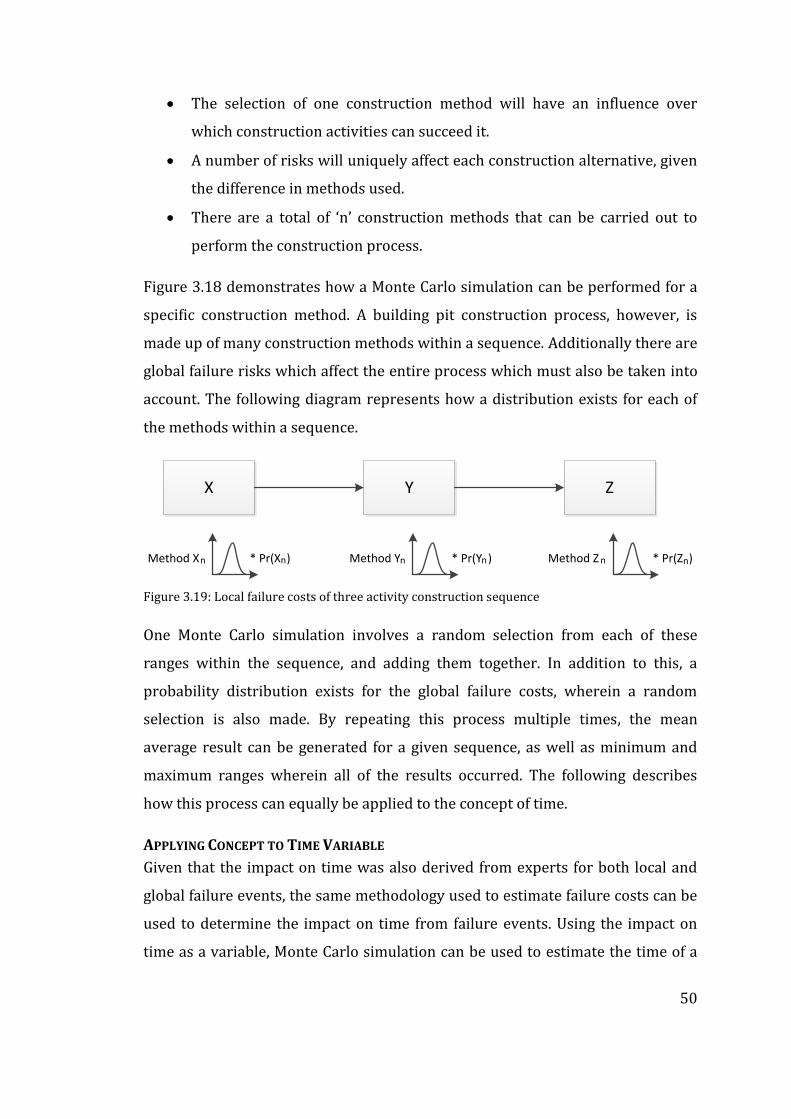
50

The selection of one construction method will have an influence over

which construction activities can succeed it.

A number of risks will uniquely affect each construction alternative, given

the difference in methods used.

There are a total of ‘n’ construction methods that can be carried out to

perform the construction process.

Figure 3.18 demonstrates how a Monte Carlo simulation can be performed for a

specific construction method. A building pit construction process, however, is

made up of many construction methods within a sequence. Additionally there are

global failure risks which affect the entire process which must also be taken into

account. The following diagram represents how a distribution exists for each of

the methods within a sequence.

X Y Z

Method Xn n Method Yn n Method Zn n* Pr(X )n * Pr(Y )n * Pr(Z )n

Figure 3.19: Local failure costs of three activity construction sequence

One Monte Carlo simulation involves a random selection from each of these

ranges within the sequence, and adding them together. In addition to this, a

probability distribution exists for the global failure costs, wherein a random

selection is also made. By repeating this process multiple times, the mean

average result can be generated for a given sequence, as well as minimum and

maximum ranges wherein all of the results occurred. The following describes

how this process can equally be applied to the concept of time.

APPLYING CONCEPT TO TIME VARIABLE

Given that the impact on time was also derived from experts for both local and

global failure events, the same methodology used to estimate failure costs can be

used to determine the impact on time from failure events. Using the impact on

time as a variable, Monte Carlo simulation can be used to estimate the time of a

51

construction sequence, incorporating the risk of failure. The impact on time of

global failures will similarly be based on the process as a whole, and must be

performed after the local failure time impacts have been assessed.

3.7 STAGE 7: ANALYSIS OF RESULTS

Upon completion of the simulations, analysis of the results is required. A graph is

generated which displays a wealth of information, the most important however

being the mean total cost, and the range width.

The mean total cost is the mean average of all of the simulations. Essentially, this

indicated which construction sequence is most likely to be the cheapest, based on

an estimation of the activity costs, and incorporating the risk of failure and its

subsequent impact on cost.

The range width indicated the range of the results, from lowest total cost to the

highest total cost for a given construction sequence. This is important because it

provides insight into the risk involved in a project, and its susceptibility to higher

costs.

The strength of this model is its ability to consider risk and its potential effect on

the total cost. Analysis of the results requires apt judgement on behalf of the

Project Manager in not only considering the mean total cost, but also considering

the variation in risk as indicated by the range width.

52

4.0 MODEL OUTPUT

The following output is from a theoretical test case for a building pit construction

project, using the proposed model. In this example, both sequence 1 (dry) and

sequence 3 (wet) have theoretically been opted for as plausible solutions (See

Figure 3.13). Additionally, the following construction methods have theoretically

been considered as being feasible:

- Wall construction: Berliner wall, driven

- Pit foundation: Concrete prefabricated pile, Hollowed steel pile, Betonnen

schalkelpaal, Steel pipes, and MV-piles

Based on this input, the following process networks can be devised:

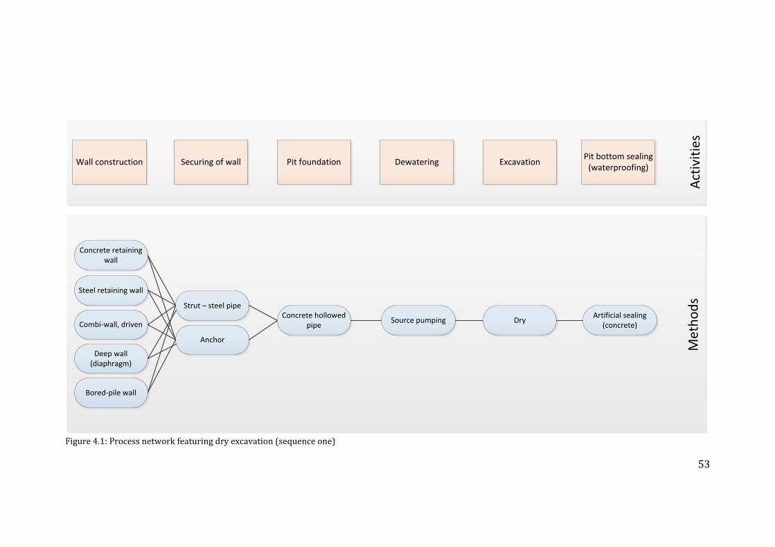
53

Wall constructionPit bottom sealing

(waterproofing)Pit foundationSecuring of wall Dewatering

Concrete retaining wall

Steel retaining wall

Combi-wall, driven

Deep wall (diaphragm)

Bored-pile wall

Artificial sealing (concrete)

Strut – steel pipe

Anchor

Met

ho

ds

Act

ivit

ies

Concrete hollowed pipe

Excavation

DrySource pumping

Figure 4.1: Process network featuring dry excavation (sequence one)

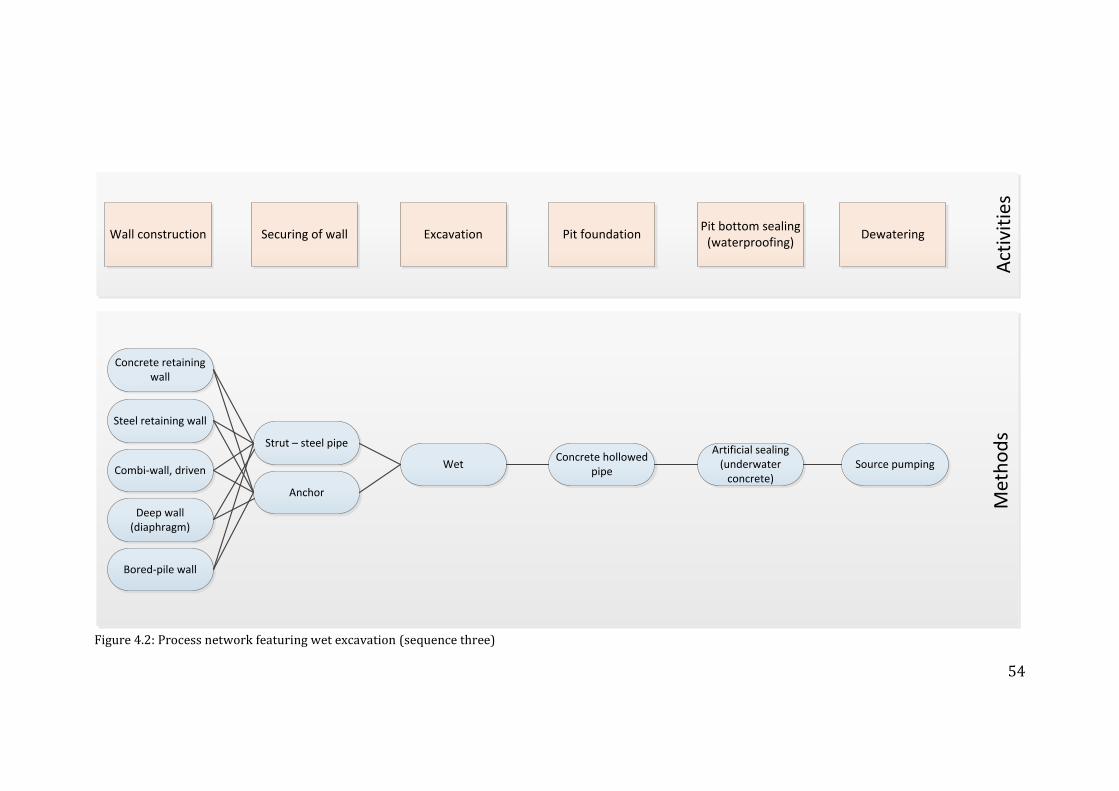
54

Wall construction DewateringExcavationSecuring of wall Pit foundation

Concrete retaining wall

Steel retaining wall

Combi-wall, driven

Deep wall (diaphragm)

Bored-pile wall

Source pumping

Strut – steel pipe

Anchor

Met

ho

ds

Act

ivit

ies

Wet

Pit bottom sealing (waterproofing)

Artificial sealing (underwater

concrete)

Concrete hollowed pipe

Figure 4.2: Process network featuring wet excavation (sequence three)

55

As can be seen from Figures 4.1 and 4.2, there are ten alternative sequences for

both the dry and wet excavation methods, amounting to twenty alternative

sequences. Having defined the project and process parameters, their

relationships, and generated plausible sequences, Monte Carlo simulation can be

performed. The following table displays the output of these results after 10,000

iterations, in order ascending of lowest mean cost risk profile.

Table 4.1: Output of Monte Carlo Simulation for all cost alternatives

STATISTICS MEAN STANDARD

DEVIATION MAXIMUM RANGE

WIDTH

Total Cost Alternative 7 128,753.19 175,629.27 1,355,620.03 1,355,620.03

Total Cost Alternative 8 133,079.39 178,859.43 1,400,379.53 1,400,379.53

Total Cost Alternative 2 136,586.26 172,396.10 1,191,880.05 1,191,880.05

Total Cost Alternative 1 138,211.68 177,033.01 1,202,329.91 1,202,329.91

Total Cost Alternative 9 139,899.47 185,102.28 1,415,317.45 1,415,317.45

Total Cost Alternative 10 141,257.09 183,285.02 1,427,459.34 1,427,459.34

Total Cost Alternative 3 142,694.99 174,806.49 1,177,203.27 1,177,203.27

Total Cost Alternative 5 143,244.29 177,727.40 1,355,313.32 1,355,313.32

Total Cost Alternative 4 146,628.98 176,277.58 1,185,061.26 1,185,061.26

Total Cost Alternative 6 148,385.63 180,036.59 1,347,484.08 1,347,484.08

Total Cost Alternative 17 149,703.91 194,875.28 1,849,634.29 1,849,634.29

Total Cost Alternative 18 153,479.04 196,160.11 1,581,046.84 1,581,046.84

Total Cost Alternative 11 157,109.84 193,487.34 1,480,550.56 1,480,550.56

Total Cost Alternative 19 161,983.91 202,537.94 1,480,720.59 1,480,720.59

Total Cost Alternative 20 162,772.09 200,452.22 1,424,500.26 1,424,500.26

Total Cost Alternative 12 163,922.94 196,744.49 1,519,715.30 1,519,715.30

Total Cost Alternative 13 165,311.85 194,144.30 1,506,523.59 1,506,523.59

Total Cost Alternative 15 165,705.03 192,497.92 1,416,119.33 1,416,119.33

Total Cost Alternative 16 167,374.39 192,582.85 1,316,253.82 1,316,253.82

Total Cost Alternative 14 170,905.01 200,389.21 1,583,981.29 1,583,981.29

The following distribution graph graphically represents the total cost for each of

the 20 alternatives, as well as the range width wherein the result yielded.

56

Figure 4.3: Distribution graph for all cost alternatives

Table 4.1 lists the alternative sequences in ascending order according to their

mean total costs. The output shows us that Alternative 7 is estimated to have the

lowest total cost. The range width however shows it to be more susceptible to

risk that some of the other cost alternatives. Alternatives 1 and 2, for example,

both yield similarly low cost estimates, yet have much smaller variations in risk.

These two alternatives may therefore be considered as favourable options given

both their low cost, and low susceptibility to risk.

57

5.0 DISCUSSION

The output of this model provides as a decision support tool for the selection of

construction sequences in building pit construction. It does this by using Monte

Carlo simulation to predict the mean total cost inclusive of failure risks. In

comparing the results of the different sequences, it is apparent that there are

huge variations in relation to the mean costs and risk variations.

There are significant differences when comparing the total mean costs of the

different sequences. Also, some sequences display a low total mean cost, yet yield

large variations in risk. Others, however, yield high total mean costs, yet

represent safe options given their relative low amount of risk. Because these

results vary so much, the most striking realisation is the impracticability in

relying on Project Managers’ intuition in selecting a construction sequence.

Additionally, only twenty alternative sequences were tested in this study, yet

some construction processes may comprise of hundreds of alternative sequences.

Without a tool which can assess these costs and associated risks, it would be

difficult to select a construction sequence with confidence that it is cost effective

and low-risk, relative to the other potential sequences.

From a Project Manager’s perspective, this model could represent a

breakthrough in construction sequence selection in building pit construction

projects. By assessing the costs and risk associated with failure of multiple

construction methods and sequences, this model can take the guesswork out of

construction sequence selection. Given the complexity and high risk involved

with building pit construction projects, a tool which quantifies such risk, and

promotes objective decision making to lower it is exactly what the industry is in

need of.

It is not possible to confirm that this model is accurate given that time restriction

meant that it could not be tested on real projects. Future studies must apply this

model to past completed projects to test its validity. In order to do so, extensive

cost and risk related data specific to that project would need to be obtained. If

such proposal is deemed to be impractical, the model could be tested on a

58

prospective project. The results of the model could then be compared to those of

the project upon its completion.

59

6.0 CONCLUSIONS

All too often Project Managers base their selection of a construction sequence on

past experience or intuition. If a project fail to meet its time, cost or quality

objectives as a result of failures, the finger will often be pointed at the

subcontractors overlooking those trades. Failure, however, is always a

possibility. As such, construction sequence selection must be grounded in a

proactive risk assessment approach which assessing the impact of failure.

The proposed risk simulation model provides an effective means assessing the

risk related to time, cost and quality of building pit construction projects. The

time and cost consequences of failures are determined based on expert advice,

and used as input for Monte Carlo simulation which realistically predicts their

occurrence. This method takes into consideration the failure events’ probabilities

and creates cost profiles inclusive of risk for every sequence conceivable. This

approach ensures that every possible sequence is assessed according to

comprehensive, quantitative risk analysis.

Drawbacks of this model, however, do exist. Firstly, the data collection process is

extensive, and the risk data that is obtained is based on subjective opinion. This

data may need to be adjusted over time after completing projects in order to

represent more realistic probabilities. Also, cost ranges have been used to

determine the impact on the cost of failures in this study. It is advisable, however,

to use up to date cost data of failure impacts in order to generate applicable

results. The comprehensiveness of the model may also be deemed as a drawback

for some observants. As shown, closed building pit construction projects can

yield hundreds of plausible alternative construction sequences. Running

simulations for each of these sequences would require far too much time for any

construction contractor to consider adopting the model. To counter this

drawback, Microsoft Excel in combination with Microsoft Visual Basic have been

used to provide a means of filtering and selecting suitable alternatives based on

the project and process parameters. Although setting up and coding this

framework requires forethought and time, it later functions as a program which

60

instantly generates all possible sequences. Upon generating the sequences,

Oracle Crystal Ball, an Excel add-on which performs probability distributions, can

be automatically instructed to perform Monte Carlo simulations using Visual

Basic. This study researches the fundamental principles of the model, however,

the means of applying it and having it autonomously function is at the discretion

of the user.

Use of the model is not specifically restricted to the building pit construction

process. The model could be equally effective in assessing the risk in other

systems which comprise of varying sequences of procurement and wherein

failure costs can occur. The strength of this model is in its ability to assess an

overwhelming spectrum of risk. Just because a Project Manager may have

worked on several similar projects in the past, does not mean they can

comprehend the risks associated with hundreds of alternative construction

sequences. This model bridges that gap, and provides a means of simulating risk

in order to assess failure costs of prospective projects.

The proposed model is promising given that it logically and systematically

quantifies a large body of risk. It can simulate the potential risk of failure and

resultant failure costs, ultimately providing as a decision-support tool for

geotechnical construction projects. Given that the model has not been tested

against real projects, however, the accuracy of its results cannot be vouched for.

As such, future work on this model must test it against the risk-related data of

real projects.

61

7.0 BIBLIOGRAPHY

AKINTOYE, A. S. & MACLOED, M. J. 1997. RISK ANALYSIS AND MANAGEMENT IN

CONSTRUCTION. INTERNATIONAL JOURNAL OF PROJECT MANAGEMENT, 15, 31-38.

AOIEONG, R. T., TANG, S. L. & AHMED, S. M. 2002. A PROCESS APPROACH IN MEASURING

QUALITY COSTS OF CONSTRUCTION PROJECTS: MODEL DEVELOPMENT. CONSTRUCTION

MANAGEMENT AND ECONOMICS, 20, 179-192.

BOURN, J. 2001. MODERNISING CONSTRUCTION. 2000-2001 ED.: NATIONAL AUDIT OFFICE.

CASTILLO, J. E. A., AL-JIBOURI, S. H. & HALMAN, J. I. M. 2009. UNDERLYING

MECHANISMS OF FAILURE COSTS IN CONSTRUCTION. UNIVERSITY OF TWENTE.

CEEP N.D. RISK ASSESSMENT TOOL FOR MEDICAL FACILITIES. CENTRE FOR EXCELLENCE IN

EMERGENCY PREPAREDNESS.

DAWOOD, N. 1998. ESTIMATING PROJECT AND ACTIVITY DURATION: A RISK MANAGEMENT

APPROACH USING NETWORK ANALYSIS. CONSTRUCTION MANAGEMENT AND ECONOMICS, 16, 41-

48.

DOLOI, H., SAWHNEY, A., IYER, K. C. & RENTALA, S. 2012. ANALYSING FACTORS

AFFECTING DELAYS IN INDIAN CONSTRUCTION PROJECTS. INTERNATIONAL JOURNAL OF PROJECT

MANAGEMENT, 30, 479-489.

EVANS, J. R. & LINDSAY, W. M. 2005. THE MANAGEMENT AND CONTROL OF QUALITY,

MASON, OH, SOUTH-WESTERN COLLEGE PUB.

FRIMPONG, Y., OLUWOYE, J. & CRAWFORD, L. 2003. CAUSES OF DELAY AND COST

OVERRUNS IN CONSTRUCTION OF GROUNDWATER PROJECTS IN A DEVELOPING COUNTRIES;

GHANA AS A CASE STUDY. INTERNATIONAL JOURNAL OF PROJECT MANAGEMENT, 21, 321-326.

HEGAZY, T., SAID, M. & KASSAB, M. 2011. INCORPORATING REWORK INTO CONSTRUCTION

SCHEDULE ANALYSIS. AUTOMATION IN CONSTRUCTION, 20, 1051-1059.

HOONAKKER, P. N.D. QUALITY MANAGEMENT IN CONSTRUCTION INDUSTRY. CENTER FOR

QUALITY AND PRODUCTIVITY IMPROVEMENT (CQPI): UNIVERSITY OF WISCONSIN-MADISON.

62

HWANG, B.-G., THOMAS, S. R., HAAS, C. T. & CALDAS, C. H. 2009. MEASURING THE

IMPACT OF REWORK ON CONSTRUCTION COST PERFORMANCE. JOURNAL OF CONSTRUCTION

ENGINEERING AND MANAGEMENT, 187-198.

IMBEAH, W. & GUIKEMA, S. 2009. MANAGING CONSTRUCTION PROJECTS USING THE

ADVANCED PROGRAMMATIC RISK ANALYSIS AND MANAGEMENT MODEL. JOURNAL OF

CONSTRUCTION ENGINEERING AND MANAGEMENT, 772-781.

IMBEAH, W. K. A. 2007. ASSESSMENT OF THE EFFECTIVENESS OF THE ADVANCED

PROGRAMMATIC RISK ANALYSIS AND MANAGEMENT MODEL (APRAM) AS A DECISION SUPPPORT

TOOL FOR CONSTRUCTION PROJECTS. TEXAS A&M UNIVERSITY.

JURAN, J. M. & GRYNA, F. M. 1988. JURAN'S QUALITY CONTROL HANDBOOK, NEW YORK,

MCGRAW-HILL

LIU, H.-T. & TSAI, Y.-L. 2012. A FUZZY RISK ASSESSMENT APPROACH FOR OCCUPATIONAL

HAZARDS IN THE CONSTRUCTION INDUSTRY. SAFETY SCIENCE, 50, 1067-1078.

LOVE, P. E. D., EDWARDS, D. J., IRANI, Z. & WALKER, D. H. T. 2009. PROJECT

PATHOGENS: THE ANATOMY OF OMISSION ERRORS IN CONSTRUCTION AND RESOURCE

ENGINEERING PROJECT. IEEE TRANSACTIONS ON ENGINEERING MANAGEMENT, 56, 425-435.

LOVE, P. E. D. & IRANI, Z. 2003. A PROJECT MANAGEMENT QUALITY COST INFORMATION

SYSTEM FOR THE CONSTRUCTION INDUSTRY. INFORMATION & MANAGEMENT, 40, 649-661.

LOVE, P. E. D. & LI, H. 2000. QUANTIFYING THE CAUSES AND COSTS OF REWORK IN

CONSTRUCTION. CONSTRUCTION MANAGEMENT AND ECONOMICS, 18, 479-490.

LOVE, P. E. D., LOPEZ, R., GOH, Y. M. & DAVIS, P. R. 2011. SYSTEMIC MODELLING OF

DESIGN ERROR CAUSATION IN SOCIAL INFRASTRUCTURE PROJECTS. PROCEDIA ENGINEERING,

14, 161-168.

LUU, V. T., KIM, S.-Y. & HUYNH, T.-A. 2008. IMPROVING PROJECT MANAGEMENT

PERFORMANCE OF LARGE CONTRACTORS USING BENCHMARKING APPROACH. INTERNATIONAL

JOURNAL OF PROJECT MANAGEMENT, 26, 758-769.

63

MAHANT, N. 2004. RISK ASSESSMENT IS FUZZY BUSINESS – FUZZY LOGIC PROVIDES THE

WAY TO ASSESS OFF-SITE RISK FROM INDUSTRIAL INSTALLATIONS. BRISBANE, AUSTRALIA:

BECHTEL CORPORATION.

MAK, S. & PICKEN, D. 2000. USING RISK ANALYSIS TO DETERMINE CONSTRUCTION PROJECT

CONTINGENCIES. JOURNAL OF CONSTRUCTION ENGINEERING AND MANAGEMENT,

MARCH/APRIL, 130-136.

MALCOLM, D. G., ROSEBOOM, J. H., CLARK, C. E. & FAZAR, W. 1959. APPLICATION OF A

TECHNIQUE FOR RESEARCH AND DEVELOPMENT PROGRAM EVALUATION. RESEARCH AND

DEVELOPMENT PROGRAM EVALUATION, 646-669.

MCINTYRE, C. & KIRSCHENMAN, M. 2000. SURVEY OF TQM IN CONSTRUCTION INDUSTRY

IN UPPER MIDWEST. JOURNAL OF MANAGEMENT IN ENGINEERING, 16, 67-70.

MINATO, T. & ASHLEY, D. B. 1998. DATA-DRIVEN ANALYSIS OF "CORPORATE RISK" USING

HISTORICAL COST-CONTROL DATA. JOURNAL OF CONSTRUCTION ENGINEERING AND

MANAGEMENT, JANUARY/FEBRUARY, 42-47.

MULHOLLAND, B. & CHRISTIAN, J. 1999. RISK ASSESSMENT IN CONSTRUCTION

SCHEDULES. JOURNAL OF CONSTRUCTION ENGINEERING AND MANAGEMENT,

JANUARY/FEBRUARY, 8-15.

OUDE VRIELINK, M. A. 2011. GEOTECHNISCH FALEN: OORZAKEN EN

BEHEERSMAATREGELEN. ENSCHEDE: UNIVERSITY OF TWENTE.

OZTAS, A. & OKMEN, O. 2004. JUDGMENTAL RISK ANALYSIS PROCESS DEVELOPMENT IN

CONSTRUCTION PROJECTS. BUILDING AND ENVIRONMENT, 40, 1244-1254.

RAMANATHAN, C., NARAYANAN, S. P. & IDRUS, A. J. 2012. CONSTRUCTION DELAYS

CAUSING RISKS ON TIME AND COST - A CRITICAL REVIEW. AUSTRALASIAN JOURNAL OF

CONSTRUCTION ECONOMICS AND BUILDING, 12, 35-57.

REZAEI, A. R., ÇELIK, T. & BAALOUSHA, Y. 2011. PERFORMANCE MEASUREMENT IN A

QUALITY MANAGEMENT SYSTEM. SCIENTIA IRANICA, TRANSACTIONS E: INDUSTRIAL

ENGINEERING, 18, 742-752.

64

ROMAN, D. 1962. THE PERT SYSTEM: AN APPRAISAL OF PROGRAM EVALUATION REVIEW

TECHNIQUE. THE JOURNAL OF THE ACADEMY OF MANAGEMENT, 5, 57-65.

SBR 2007. HANDBOEK FUNDERINGSHERSTEL.

SIEGEL, S. & JOHN CASTELLAN, N. 1988. NONPARAMETRIC STATISTICS FOR THE

BEHAVIORAL SCIENCES, NEW YORK, MCGRAW-HIL.

SOARES, C. G. 1997. ADVANCES IN SAFETY AND RELIABILITY : PROCEEDINGS OF THE ESREL '97

INTERNATIONAL CONFERENCE ON SAFETY AND RELIABILITY, OXFORD.

TALON, A., BOISSIER, D., HANS, J., LACASSE, M. A. & CHORIER, J. FMECA AND

MANAGEMENT OF BUILDING COMPONENTS. INTERNATIONAL CONFERENCE ON DURABILITY OF

BUILDING MATERIALS AND COMPONENTS, MAY 11, 2008 2008 ISTANBUL, TURKEY.

NATIONAL RESEARCH COUNCIL CANADA.

WILLMER, G. 1991. TIME AND COST RISK ANALYSIS. COMPUTERS & STRUCTURES, 41, 1149-

1155.

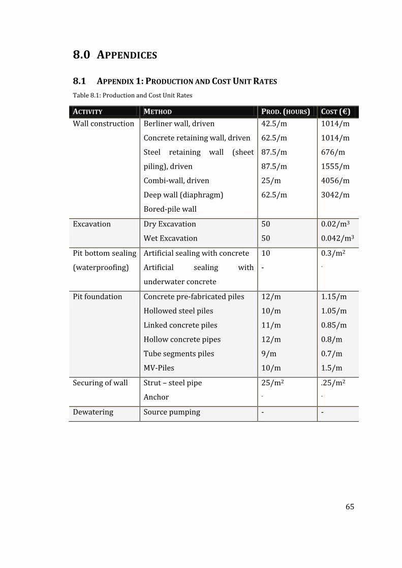
65

8.0 APPENDICES

8.1 APPENDIX 1: PRODUCTION AND COST UNIT RATES

Table 8.1: Production and Cost Unit Rates

ACTIVITY METHOD PROD. (HOURS) COST (€)

Wall construction Berliner wall, driven

Concrete retaining wall, driven

Steel retaining wall (sheet

piling), driven

Combi-wall, driven

Deep wall (diaphragm)

Bored-pile wall

42.5/m

62.5/m

87.5/m

87.5/m

25/m

62.5/m

1014/m

1014/m

676/m

1555/m

4056/m

3042/m

Excavation Dry Excavation

Wet Excavation

50

50

0.02/m3

0.042/m3

Pit bottom sealing

(waterproofing)

Artificial sealing with concrete

Artificial sealing with

underwater concrete

10

-

0.3/m2

-

Pit foundation Concrete pre-fabricated piles

Hollowed steel piles

Linked concrete piles

Hollow concrete pipes

Tube segments piles

MV-Piles

12/m

10/m

11/m

12/m

9/m

10/m

1.15/m

1.05/m

0.85/m

0.8/m

0.7/m

1.5/m

Securing of wall Strut – steel pipe

Anchor

25/m2

-

.25/m2

-

Dewatering Source pumping - -

66

8.2 APPENDIX 2: EXPERT REMARKS ON ACTIVITIES

Table 8.2: Expert Remarks on Activities

ACTIVITY REMARK

Wall construction Based on installation costs, Sheet-wall installation costs

represent a quarter of the installation costs of Diaphragm

walls;

“The difference in costs between Sheet piling and diaphragm

wall affects the decision to accept certain risks. For example

the ratio in costs maybe 1EUR of sheet wall cost over 4EUR

of diaphragm wall. So if the risk of using sheet pile is around

10 to 20%, it is still cheaper to use sheet pile against DW”

Based on production rate, Sheet-walls are installed faster

than Diaphragm wall. Sheet wall production rate is between

300m2 and 400m2 per day, whereas Diaphragm wall

production rate ranges between 80m2 to 100m2 per day;

Wall construction based on driven methods are associated

with high risk for damaging the surroundings;

Bored pile walls are not suitable for depth of more than 6m

because of its high probability for not being sealed. This

happens when the bored piles being constructed deviate

from the vertical axis during construction and this may lead

to failures such as filtration of water and ground;

Concrete and steel retaining walls are more suitable for soft

soil;

Diaphragm walls are suitable in hard soil, but can be used in

soft soil in case vibration is not tolerable.

Securing of wall The use of anchors is preferred against the use of struts,

unless there is a legal/technical objections for using anchors,

e.g. buildings near-by;

Pit foundation When foundation piles need to be installed inside the pit you

can either install them before a dry excavation or after a wet

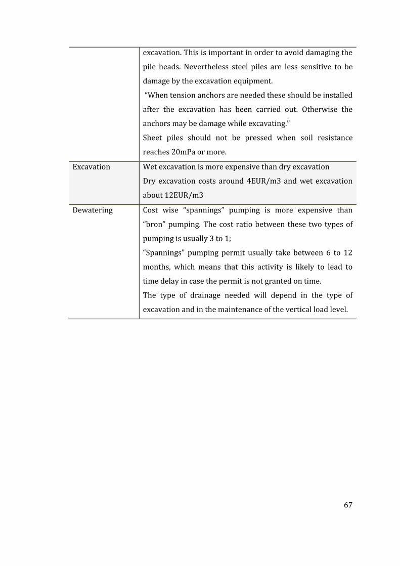
67

excavation. This is important in order to avoid damaging the

pile heads. Nevertheless steel piles are less sensitive to be

damage by the excavation equipment.

“When tension anchors are needed these should be installed

after the excavation has been carried out. Otherwise the

anchors may be damage while excavating.”

Sheet piles should not be pressed when soil resistance

reaches 20mPa or more.

Excavation Wet excavation is more expensive than dry excavation

Dry excavation costs around 4EUR/m3 and wet excavation

about 12EUR/m3

Dewatering Cost wise “spannings” pumping is more expensive than

“bron” pumping. The cost ratio between these two types of

pumping is usually 3 to 1;

“Spannings” pumping permit usually take between 6 to 12

months, which means that this activity is likely to lead to

time delay in case the permit is not granted on time.

The type of drainage needed will depend in the type of

excavation and in the maintenance of the vertical load level.

68

8.3 APPENDIX 3: LOCAL FAILURE RISKS

Table 8.3: Local Failure Risks

LOCAL RISK

Sheet pile is not at the correct depth

Sheet pile is out of the lock

Damage to the sheet pile

Insufficient waterproofing wall

Cement bentonite wall not cured enough

Did not arrive at the correct depth pile wall

Slot instability

Instability pile wall section

Overconsumption of concrete

Different element size

Abnormal strength of element

Do not arrive at depth element

Do not arrive at depth anchoring

Succumb stamp / anchor / purlin

Different size / strength / stiffness anchor

Tearing or perforation

Thickness floor is too small

Diameter / height shielded insufficient

Flooding caused by drainage failure

Insufficient overlap of elements

Injection material is washed away

Did not arrive at depth pile

Different quality pile

Different pile capacity

Bases is not compacted

Drainage failure due to wear, clogging, vandalism, etc.

Instability (collapse) wall

69

Leakage / excavation through holes in wall

Leakage / excavation through holes in floor

By collapsing wall collapse stamp / anchor / purlin

Uplifting pit floor / floor increase

Succumb foundation element

Ground deformation and adjoining recreation ground by drilling or by injection

(only sheet piling)

Ground deformation and adjoining properties by compaction / relaxation by

ground vibration / drilling of the wall / foundation element

Ground deformation and adjoining properties by surface relaxation by jet

grouting next foundation

Deformation under load and adjoining properties by influencing neighbouring

foundations by drilling in anchors

Deformation and adjoining land by large deformation / failure of wall / strut /

anchor / purlin

Deformation and adjoining land by excavation or leakage through holes in wall

Ground deformation and adjoining properties due to leakage / uplifting by

excavation pit floor or heaving