A risk attitudinal ranking method for interval-valued

intuitionistic fuzzy numbers based on novel attitudinal expected

score and accuracy functions

Jian Wua,b, Francisco Chiclanab

aSchool of Economics and Management, Zhejiang Normal University, Jinhua, Zhejiang, ChinabCentre for Computational Intelligence, Faculty of Technology, De Montfort University, Leicester, UK

Abstract

This article investigates new score and accuracy functions for ranking interval-valued

intuitionistic fuzzy numbers (IVIFNs). The novelty of these functions is that they allow

the comparison of IVIFNs by taking into account of the decision makers’ attitudinal

character. The new attitudinal expected score and accuracy functions extend Xu and

Chen’s score and accuracy degree functions, and verify the following set of properties:

(1) boundedness; (2) monotonicity; (3) commutativity; and (4) symmetry. These novel

functions are used to propose a total order on the set of IVIFNs, and to develop an

interval-valued intuitionistic fuzzy multi-attribute decision making selection process in

which the final result depends on the decision maker’s risk attitude. In addition, a

ranking sensitivity analysis with respect to the risk attitude is provided.

Keywords: Multi-attribute decision-making, interval-valued intuitionistic sets,

attitudinal expected score function, attitudinal expected accuracy function, COWA

operator

1. Introduction

Atanassov [1] introduced the concept of intuitionistic fuzzy sets (IFSs), which is char-

acterised by both the membership and non-membership functions and therefore it gener-

alises the concept of fuzzy set [2, 3]. Subsequently, Atanassov and Gargov [4] extended

IFSs with the introduction of the concept of interval-valued intuitionistic fuzzy sets (IV-

IFSs). The notions of IFSs and IVIFSs are interesting and very useful in modelling

real life problems with imprecision or uncertainty and they have been applied to many

Email addresses: jyajian@163.com (Jian Wu), chiclana@dmu.ac.uk (Francisco Chiclana)

Preprint submitted to Applied Soft Computing. Accepted on May 2014 May 9, 2014

different fields, including multiple attribute decision making (MADM) [5–9], group deci-

sion making (GDM) [10–12], supplier selection [13, 14], robot selection [15] and artificial

intelligence [16].

The first step of any MADM process with information modelled using IFSs is to

fuse the intuitionistic fuzzy assessment values of the different attributes into a collective

intuitionistic fuzzy assessment via an appropriate aggregation operator [17]. Once this

step has been completed, the aggregated intuitionistic fuzzy numbers are compared to

produce a final ranking of the alternatives. Consequently, an active research topic is the

investigation of intuitionistic fuzzy MADM that includes suitable and valid intuitionistic

fuzzy aggregation operators. Since Xu [18] developed the intuitionistic fuzzy ordered

weighted averaging (IFOWA) operator, extensive research work has been carried out to

develop aggregation operators for both IFSs and/or IVIFSs (see for example [19–21]).

However, the above cited intuitionistic fuzzy operators are based on additive measures

and are not suitable to aggregate inter-dependent criteria. To resolve this issue, Tan

and Chen [22, 23] proposed the intuitionistic fuzzy Choquet integral operator and the

generalized interval-valued intuitionistic fuzzy geometric aggregation operator for multi-

attribute interval-valued intuitionistic fuzzy group decision making problems.

Another active research topic regards the development of score degree and accuracy

degree functions to make possible the comparison of criterion values that are expressed

by IFSs and IVIFSs, respectively. A comprehensive comparative analysis of existing score

degree and accuracy degree functions to date can be found in [24]. Chen and Tan in [25]

developed a score degree function for IFSs based on the membership degree and non-

membership degree functions, which was later improved by Hong and Choi in [26] with

the addition of an accuracy degree function. In addition, Hong and Choi argued about

the similarity between the role of the score degree and the accuracy degree functions of

IFSs and that of the mean and the variance in statistics. Subsequently, other improved

score degree and accuracy degree functions have been proposed in [27–32]. Also these

functions are extended to the cases of triangular intuitionistic fuzzy numbers [33, 34]

and intuitionistic linguistic numbers [35–37]. It is worth mentioning the score degree and

accuracy degree functions recently developed by Xu and Chen in [38] to propose an order

relation on the set of interval-valued intuitionistic fuzzy numbers (IVIFNs). However, as

it will be proved later with a counter-example (Example 1), the order relation derived

2

from the application of Xu and Chen’s score degree and accuracy degree functions is

not total. In a attempt to resolve this drawback, Ye in [39] and Lakshmana Gomathi

Nayagam in [40] proposed alternative accuracy degree functions, respectively, which they

claimed produced a total ordering of IVIFNs. However, these alternative degree functions

are not superior to the existing accuracy degree functions but equivalent ‘in the course

of comparing any two interval-valued intuitionistic fuzzy numbers’. As it will be shown

later in Section 3.3, these score degree and accuracy degree functions do not capture well

all the information contained in IVIFNs and consequently can lead to a lack of precision

in the final ordering of IVIFNs. We believe that this is because these functions are simple

and straight forward extensions of their respective proposals for the case of IFNs. An

important limitation of the above approaches resides in the fact that they do not take into

account the attitudinal character of decision makers. Yager in [41] pointed out that the

attitudinal character of each decision maker may affect the final ranking order of fuzzy

numbers (FNs). The problem of ordering FNs, though, has been extensively studied and

an agreed conclusion is that there is no unique best approach to do this. Recall that FNs

are particular cases of IVIFNs. Thus, the same conclusion applies to IVIFNs. Therefore,

it is important to develop a methodology that best captures the decision maker’s risk

attitude regarding the ranking IVIFNs.

In order to achieve this, the the remainder of this paper is organised as follows: The

next section briefly reviews the main score degree and accuracy degree functions of IVIFSs

and an analysis of their relationships as well as their associated drawbacks is carried out,

which it is used in Section 3 to support the development of novel attitudinal expected score

and accuracy functions of IVIFNs driven by the decision maker’s attitudinal character. In

this section, it is also proved that the new attitudinal expected functions extend Xu and

Chen’s score degree and accuracy degree functions. The following desirable properties

are proved to be satisfied by the new attitudinal expected functions: (i) boundedness;

(ii) monotonicity; (iii) commutativity; and (iv) symmetry. This section is completed

with the definition of a total order relation on the set of IVIFNs. Section 4 presents

a sensitivity analysis with respect to the attitudinal character and a resolution process

of MADM problems in an interval-valued intuitionistic fuzzy environment. Finally, in

Section 5 conclusions are drawn and suggestions made for further work.

3

2. Preliminaries

This section presents the key concepts related to IVIFSs that will be used throughout

this paper. First, we present Atanassov and Gargov’s defintion of the notion of IVIFS,

which is characterised by a membership function and a non-membership function that

take interval numbers rather than crisp numbers, as introduced in [4].

Definition 1 (Interval-Valued IFS (IVIFS)). Let INT ([0, 1]) be the set of all closed

subintervals of the unit interval and X be a universe of discourse. An interval-valued IFS

(IVIFS) A over X is given as:

A ={〈x, µA(x), νA(x)〉 |x ∈ X

}(1)

where µA(x), νA(x) ∈ INT ([0, 1]), represent the membership and the non-membership

degrees of the element x to the set A subject to the following constraint

0 ≤ sup µA(x) + sup νA(x) ≤ 1,∀x ∈ X.

Denoting by µAL(x), µAU(x), νAL(x) and νAU(x) the lower and upper end points of

µA(x) and νA(x), respectively, an IVIFS can be represented as

A ={⟨x, [µAL(x), µAU (x)],[νAL(x), νAU (x)]

⟩∣∣x ∈ X : 0 ≤ µAU (x) + νAU (x) ≤ 1, µAL(x) ∧ νAL(x) ≥ 0

}(2)

Recall that given two IVIFSs, A and B, Atanassov and Gargov containment concept

is modelled as follows [4]:

A ⊆ B

iff

∀x ∈ X : µAL(x) ≤ µBL(x) ∧ µAU(x) ≤ µBU(x) ∧ νAL(x) ≥ νBL(x) ∧ νAU(x) ≥ νBU(x).

The hesitancy degree function of an IVIFS is:

πA(x) = [1− µAU(x)− νAU(x), 1− µAL(x)− νAL(x)]. (3)

Given x ∈ X,

([µAL(x), µAU(x)], [νAL(x), νAU(x)])

4

will be referred to as an interval-valued intuitionistic fuzzy number (IVIFN). For conve-

nience, an IVIFN will be denoted by ([µ−, µ+], [ν−, ν+]).

Given two IVIFNs α1 = ([µ−1 , µ

+1 ], [ν−1 , ν

+1 ]) and α2 = ([µ−

2 , µ+2 ], [ν−2 , ν

+2 ]), we have the

following definition of containment [4]:

α1 ⊆ α2 iff µ−1 ≤ µ−

2 , µ+1 ≤ µ+

2 , ν−1 ≥ ν−2 , and ν+

1 ≥ ν+2 .

Also, the main arithmetic operations can be expressed in terms of the interval lower and

upper bounds as follows [1, 42]:

1) α1 = ([ν−1 , ν+1 ], [µ−

1 , µ+1 ])

2) α1 ⊕ α2 = ([µ−1 + µ−

2 − µ−1 · µ−

2 , µ+1 + µ+

2 − µ+1 · µ+

2 ], [ν−1 · ν−2 , ν+1 · ν+

2 ])

3) α1 ⊗ α2 = ([µ−1 · µ−

2 , µ+1 · µ+

2 ], [ν−1 + ν−2 − ν−1 · ν−2 , ν+1 + ν+

2 − ν+1 · ν+

2 ])

4) λ · α1 = ([1− (1− µ−1 )λ, 1− (1− µ+

1 )λ], [(ν−1 )λ, (ν+1 )λ])

5) αλ1 = ([(µ−1 )λ, (µ+

1 )λ], [1− (1− ν−1 )λ, 1− (1− ν+1 )λ])

The score degree and accuracy degree functions play a key role in MADM problems

with interval-valued intuitionistic fuzzy information because they allow the comparison

of criteria values using IVIFNs. For IVIFNs, Xu and Chen proposed in [38] the following

score degree and accuracy degree functions:

Definition 2 (Xu and Chen’s IVIFN Score and Accuracy Functions [38]). Let α =

([µ−, µ+], [ν−, ν+]) be an IVIFN. The score degree and accuracy degree functions of α are

represented, respectively, by

SXC(α) =µ− + µ+ − ν− − ν+

2(4)

and

AXC(α) =µ− + µ+ + ν− + ν+

2. (5)

Notice that SXC(α) ∈ [−1, 1], while AXC(α) ∈ [0, 1], and that both functions are

related as follows:

AXC(α) = SXC(α) + (ν− + ν+). (6)

Thus, the following result is proved:

5

Proposition 1. Given an IVIFN α = ([µ−, µ+], [ν−, ν+]), the following inequality holds:

SXC(α) ≤ AXC(α)

The score degree function is monotonic increasing with respect to the containment

relation of IVIFNs are the following result proves:

Proposition 2. Given two IVIFNs α1 and α2 such that α1 ⊆ α2 then it is SXC(α1) ≤

SXC(α2).

Proof. Recall that α1 ⊆ α2 is equivalent to µ−1 ≤ µ−

2 , µ+1 ≤ µ+

2 , ν−1 ≥ ν−2 , ν

+1 ≥ ν+

2 .

Therefore it is

µ−1 + µ+

1 − ν−1 − ν+1 ≤ µ−

2 + µ+2 − ν−2 − ν+

2 .

The score degree and accuracy degree are used by Xu and Chen to propose the

following IVIFNs two level ranking method:

Definition 3 (Xu amnd Chen’s IVIFNs Order Relation [38]). Given two IVIFNs

α1 = ([µ−1 , µ

+1 ], [ν−1 , ν

+1 ]) and α2 = ([µ−

2 , µ+2 ], [ν−2 , ν

+2 ]), the following ordering relation can

be established:

(1) If SXC(α1) < SXC(α2) then α1 < α2.

(2) If SXC(α1) = SXC(α2):

(i) If AXC(α1) < AXC(α2) then α1 < α2.

(ii) If AXC(α1) = AXC(α2) then α1 = α2.

In the first level, the score degree is used to rank the IVIFNs, and the second level

is only applied when two IVIFNs have same score degrees, in which case their accuracy

degrees are used to discern the order relation between the IVIFSs. Two IVIFSs are

considered equivalent in term of ordering when both have same score degree and accuracy

degree.

Ye in [39] proposed an alternative expression for the accuracy degree function of an

IVIFN to Xu and Chen’s accuarcy degree function, but with same range of values, [−1, 1]:

6

Definition 4 (Ye’s IVIFN Accuracy Function [39]). The accuracy degree function

of an IVIFN α = ([µ−, µ+], [ν−, ν+]) can be represented by

AY (α) = µ− + µ+ +ν− + ν+

2− 1 (7)

Notice that in the above definitions, the hesitancy degree function of IVIFNs is not

implemented, which is not the case in the following accuracy degree function introduced

by Lakshmana and Sivaraman in [40]:

Definition 5 (Lakshmana and Sivaraman’s IVIFN Accuracy Function [40]). The

hesitancy based accuracy degree function of an IVIFN α = ([µ−, µ+], [ν−, ν+]) can be rep-

resented by

ALSδ(α) =membership degree + δ · (hesitancy degree)

2(8)

i.e.

ALSδ(α) =µ− + µ+ + δ · (2− µ− − µ+ − ν− − ν+)

2(9)

where δ ∈ [0, 1] is a parameter that is used to control the individual’s intentions as follows:

δ = 1 corresponds to an optimistic individual, while a pessimistic one would have a value

of δ = 0.

An alternative expression for ALSδ(α) is:

ALSδ(α) =1− δ

2· (µ− + µ+)− δ

2· (ν− + ν+) + δ. (10)

Using expression (10), it is easy to prove that Lakshmana and Sivaraman’s accuracy

function is monotonic increasing with respect to the containment relation of IVIFNs:

Proposition 3. Given two IVIFNs α1 and α2 such that α1 ⊆ α2, then it is ALSδ(α1) ≤

ALSδ(α2).

Notice that AY (α) and ALSδ(α) can be re-written as follows:

AY (α) = SXC(α) +3

2· AXC(α)− 1

ALSδ(α1) =1

2· SXC(α) +

1− 2 · δ2

· AXC(α) + δ.

The following relationships between the above score degree and accuracy degree functions

are established:

7

Proposition 4. The IVIFN accuracy degree function ALSδ and the score degree function

SXC are related as follows:

ALS0.5(α) =1

2· SXC(α) +

1

2(11)

and therefore are equivalent in the ordering IVIFNs.

Proposition 5. Given any two IVIFNs α1 = ([µ−1 , µ

+1 ], [ν−1 , ν

+1 ]) and α2 = ([µ−

2 , µ+2 ], [ν−2 , ν

+2 ]),

we have:

1. If SXC(α1) = SXC(α2) and AXC(α1) = AXC(α2) then

1.a) AY (α1) = AY (α2).

1.b) ALSδ(α1) = ALSδ(α2).

2. If SXC(α1) = SXC(α2) and AXC(α1) < AXC(α2) then

2.a) AY (α1) < AY (α2).

2.b1) ALSδ(α1) < ALSδ(α2) when δ < 0.5.

2.b2) ALSδ(α1) = ALSδ(α2) when δ = 0.5.

2.b3) ALSδ(α1) > ALSδ(α2) when δ > 0.5.

As mentioned before, the score degree and accuracy degree functions are widely used

in interval-valued intuitionistic fuzzy MADM problems to produce a final ranking of al-

ternatives. However, as the following example illustrates, they are unable to discriminate

between all pairs of IVIFNs in terms of ranking:

Example 1. The following two IVIFNs

α1 = ([0.15, 0.35], [0.2, 0.4]) and α2 = ([0.2, 0.3], [0.2, 0.35])

have the same score value SXC(α1) = SXC(α2) = −0.05, and therefore the accuracy value

is to be used to rank them. However, in this case we have AXC(α1) = AXC(α2) = 0.55.

From expressions (7) and (9), and in accordance to Proposition 5, we have AY (α1) =

AY (α1) = −0.025 and ALSδ(α1) = ALSδ(α2) = 0.25 + 0.45 · δ, respectively.

8

The example above manifests that the application of the reviewed score degree and

accuracy degree functions are unable to make a clear decision between two alternatives

with final evaluation represented with apparently different IVIFNs, as they treat them as

equal in terms of ordering. This drawback could be overcome by implementing the score

degree and accuracy degree functions takeing into account of the decision maker’s risk

attitude, as proposed in the following section.

3. The risk attitudinal expected score and accuracy functions

Yager [41] pointed out that the comparison of FNs is a problem that has been ex-

tensively studied and that there is no unique best approach. Indeed, the set of fuzzy

numbers is not totally ordered, and therefore a widely used approach to rank FNs con-

sists in converting them into a representative crisp value, and perform the comparison

on them [41, 43], a methodology originally proposed by Zadeh in [44]. Recently, a study

by Brunelli and Mezei [45] that compares different ranking methods for fuzzy numbers

concludes that ‘it is impossible to give a final answer to the question on what ranking

method is the best. Most of the time choosing a method rather than another is a matter

of preference or is context dependent.’ Recall that FNs are particular cases of IVIFNs.

Thus, the same conclusion applies to IVIFNs. In any case, it seems appropriate to take

into account the decision maker’s risk attitude to derive a final solution to the MADM

problem. In the following, we propose the risk attitudinal expected score and accuracy

functions for IVIFNs, which extend the functions reviewed in Section 2.

3.1. The attitudinal expected function and its properties

In the following, an interval valued score function for IVIFNs is introduced and a

novel expected score function that takes into account the decision maker’s attitude via the

application of the concept of attitudinal character of a BUM and the continuous ordered

weighted average (COWA) operator introduced by Yager [41]. A set of properties of the

attitudinal expected score function is also proved. To do this, we start by recalling the

concept of a basic unit-monotonic (BUM) function [46]:

Definition 6 (BUM function). A function Q : [0, 1] → [0, 1] such that Q(0) = 0,

Q(1) = 1 and Q(x) ≥ Q(y) if x ≥ y is called a basic unit-monotonic (BUM) function

9

Given a BUM function, Q, Yager proposed the following definition of the COWA

operators [41]:

Definition 7 (COWA Operator). Let INT (R) be the set of all closed subintervals of

R. A continuous ordered weighted average (COWA) operator is a mapping FQ : INT (R)→

R which has an associated BUM function, Q, such that

FQ ([a, b]) = (1− λ) · a+ λ · b. (12)

where

λ =

∫ 1

0

Q(y)dy. (13)

is the attitudinal character of Q. Thus, FQ ([a, b]) is the weighted average of the end

points of the closed interval with attitudinal character parameter λ, and it is known as

the attitudinal expected value of [a, b].

In the following, an interval-valued score function is proposed for IVIFNs to derive,

after the application of expression (12), the new attitudinal expected score function to

be applied in the resolution of interval-valued intuitionistic fuzzy MADM problems:

Definition 8 (IVIFN Interval-Valued Score Function). Let INT ([−1, 1]) be the

set of all closed subintervals of [−1, 1]. The interval-valued score function associated

to an IVIFN α(x) = ([µ−(x), µ+(x)], [ν−(x), ν+(x)]) is given as follows:

SWC(α) : X −→ INT ([−1, 1]),

SWC(α)(x) = [µ−(x), µ+(x)]− [ν−(x), ν+(x)] = [µ−(x)− ν+(x), µ+(x)− ν−(x)] (14)

As it was done before, we will drop the symbol x when referring to the interval-valued

score function of an IVIFN α, and it will be denoted simply as SWC(α) = [µ−− ν+, µ+−

ν−].

Definition 9 (IVIFN Attitudinal Expected Score Function). The attitudinal ex-

pected score function associated to an IVIFN α, SWC is

E(SWC(α)

)λ

= (1− λ) · (µ− − ν+) + λ · (µ+ − ν−) (15)

where λ is the attitudinal character of a BUM function Q.

10

Notice that because the attitudinal expected score function is based on the COWA

operator, some of the properties of this last one are expected to be inherited by the former

one. In the following, we provide such set of properties.

The attitudinal expected score function is monotonic with respect to the containment

relation of IVIFNs:

Proposition 6. Given any two IVIFNs α1 = ([µ−1 , µ

+1 ], [ν−1 , ν

+1 ]) and α2 = ([µ−

2 , µ+2 ], [ν−2 , ν

+2 ]),

such that

α1 ⊆ α2

then

E(SWC(α1)

)λ≤ E

(SWC(α2)

)λ.

Proof. According to Definition 9, we have

E(SWC(α1)

)λ−E

(SWC(α2)

)λ

= (1−λ)·[(µ−1 −ν+

1 )−(µ−2 −ν+

2 )]+λ·[(µ+1 −ν−1 )−(µ+

2 −ν−2 )]

Because α1 ⊆ α2 then it is µ−1 ≤ µ−

2 , µ+1 ≤ µ+

2 , ν−1 ≥ ν−2 , and ν+

1 ≥ ν+2 , and therefore

µ−1 − ν+

1 ≤ µ−2 − ν+

2 ∧ µ+1 − ν−1 ≤ µ+

2 − ν−2 .

Thus, we conclude:

E(SWC(α1)

)λ− E

(SWC(α2)

)λ≤ 0.

Notice that fixing an IVIFN α the attitudinal expected score function can be con-

sider a function of the attitudinal character λ, of which it exhibits the following type of

monotonicity property.

Proposition 7. Given an IVIFN, α = ([µ−, µ+], [ν−, ν+]), the attitudinal expected score

function E(SWC(α)

)λ

is monotonic with respect to the argument λ, i.e.

λ1 ≥ λ2 ⇒ E(SWC(α)

)λ1≥ E

(SWC(α)

)λ2.

Proof. Notice that E(SWC(α)

)λ

can be re-written as follows

E(SWC(α)

)λ

= (µ− − ν+) + λ · (µ+ − µ− + ν+ − ν−)

Because µ+−µ− +ν+−ν− ≥ 0 it is obvious that E(SWC(α)

)λ

is increasing with respect

to λ.

11

The attitudinal expected score function is also bounded.

Proposition 8. Given an IVIFN α = ([µ−, µ+], [ν−, ν+]), we have

−1 ≤ µ− − ν+ ≤ E(SWC(α)

)λ≤ µ+ − ν− ≤ 1.

Proof. From Proposition 7 we know that the minimum and maximum values ofE(SWC(α)

)λ

are obtained for λ = 0 and λ = 1, respectively. We have:

E(SWC(α)

)0

= µ− − ν+

E(SWC(α)

)1

= µ+ − ν−

This completes the proof.

From the results of the preceding theorems, we see that the attitudinal expected score

function is a mean operator. The following result proves that the attitudinal expected

score function is additive and therefore it is a weighted averaging operator.

Proposition 9. Given any two IVIFNs α1 = ([µ−1 , µ

+1 ], [ν−1 , ν

+1 ]) and α2 = ([µ−

2 , µ+2 ], [ν−2 , ν

+2 ]),

we have

E(SWC(α1) + SWC(α2)

)λ

= E(SWC(α1)

)λ

+ E(SWC(α2)

)λ

Proof. Because SWC(α1) + SWC(α2) = [(µ−1 − ν+

1 ) + (µ−2 − ν+

2 ), (µ+1 − ν−1 ) + (µ+

2 − ν−2 )]

then it is

E(SWC(α1) + SWC(α2)

)λ

= (1−λ)·[(µ−

1 − ν+1 ) + (µ−

2 − ν+2 )]+λ·

[(µ+

1 − ν−1 ) + (µ+2 − ν−2 )

].

Re-arranging the right-hand side we have

E(SWC(α1) + SWC(α2)

)λ

=[(1− λ) · (µ−

1 − ν+1 ) + λ · (µ+

1 − ν−1 )]

+[(1− λ) · (µ−

2 − ν+2 ) + λ · (µ+

2 − ν−2 )

Thus:

E(SWC(α1) + SWC(α2)

)λ

= E(SWC(α1)

)λ

+ E(SWC(α2)

)λ.

The attitudinal expected score function generalises Xu and Chen’s score function as

the following result proves:

12

Proposition 10. The IVIFN score function SXC and the IVIFN attitudinal expected

score function E(SWC(α)

)λ

are related as follows

E(SWC(α)

)0.5

= SXC(α). (16)

Proof. When λ = 0.5 the expression of E(SWC(α)

)λ

reduces to

E(SWC(α)

)0.5

=1

2· (µ− − ν+) +

1

2· (µ+ − ν−) =

µ− + µ− − ν− − ν−

2= SXC(α).

In the following we will provide a sensitivity analysis of the attitudinal expected score

function with respect to the attitudinal character λ, i.e we will provide the conditions

under which the ordering of two IVIFNs is not affected by a change in the attitudinal

parameter.

Theorem 1. Let αi = ([µ−i , µ

+i ], [ν−i , ν

+i ]) and αj = ([µ−

j , µ+j ], [ν−j , ν

+j ]) be two IVIFNs,

and let λ be the attitudinal parameter associated to BUM function Q under which it has

been established that

E(SWC(αi)

)λ≤ E

(SWC(αj)

)λ.

Let ∆λ be a perturbation of the attitudinal character λ with 0 ≤ λ + ∆λ ≤ 1. Then we

have

E(SWC(αi)

)λ+∆λ

≤ E(SWC(αj)

)λ+∆λ

iff

max

{− λ,

E(SWC(αj)

)λ− E

(SWC(αi)

)λ

βi − βj

}≤ ∆λ ≤ 1− λ, if βi < βj

−λ ≤ ∆λ ≤ 1− λ, if βj = βi

−λ ≤ ∆λ ≤ min

{1− λ,

E(SWC(αj)

)λ− E

(SWC(αi)

)λ

βi − βj

}, if βi > βj

where βi = µ+i − µ−

i + ν+i − ν−i and βj = µ+

j − µ−j + ν+

j − ν−j .

Proof. Firstly, we note that ∆λ is subject to the following constraint:

−λ ≤ ∆λ ≤ 1− λ.

13

We have the following relation between E(SWC(αi)

)λ+∆λ

and E(SWC(αi)

)λ:

E(SWC(αi)

)λ+∆λ

= E(SWC(αi)

)λ

+ ∆λ · βi

where βi = µ+i − µ−

i + ν+i − ν−i . The following equivalence holds:

E(SWC(αi)

)λ+∆λ

≤ E(SWC(αj)

)λ+∆λ

⇔ ∆λ·(βi−βj) ≤ E(SWC(αj)

)λ−E

(SWC(αi)

)λ

(17)

Three scenarios are possible:

• βi = βj. Because E(SWC(αi)

)λ≤ E

(SWC(αj)

)λ

then (17) is true for any value of

∆λ, i.e.

−λ ≤ ∆λ ≤ 1− λ.

• βi > βj ⇔ ∆λ ≤E(SWC(αj)

)λ− E

(SWC(αi)

)λ

βi − βj, and therefore:

−λ ≤ ∆λ ≤ min

{1− λ,

E(SWC(αj)

)λ− E

(SWC(αi)

)λ

βi − βj

}.

• βi < βj ⇔ ∆λ ≥E(SWC(αj)

)λ− E

(SWC(αi)

)λ

βi − βj, and therefore:

max

{− λ,

E(SWC(αj)

)λ− E

(SWC(αi)

)λ

βi − βj

}≤ ∆λ ≤ 1− λ.

3.2. The attitudinal expected accuracy function and its properties

Following the methodology of Section 3.1, an interval valued accuracy function for

IVIFNs and a novel expected accuracy function that takes into account the decision

maker’s attitude are introduced.

Definition 10 (IVIFN Interval-Valued Accuarcy Function). Let INT ([0, 1]) be the

set of all closed subintervals of [0, 1]. The interval-valued accuracy function associated to

an IVIFN, α(x) = ([µ−(x), µ+(x)], [ν−(x), ν+(x)]) is given as follows

AWC(α) : X −→ INT ([0, 1]),

14

AWC(α)(x) = [µ−(x), µ+(x)] + [ν−(x), ν+(x)] = [µ−(x) + ν−(x), µ+(x) + ν+(x)] (18)

Again, we will drop the symbol x when referring to the interval-valued accuracy function

of an IVIFN α, and it will be denoted simply as AWC(α) = [µ− + ν−, µ+ + ν+].

Definition 11 (IVIFN Attitudinal Expected Accuarcy Function). The attitudi-

nal expected accuracy function associated to an IVIFN α, AWC is

E(AWC(α)

)λ

= (1− λ) · (µ− + ν−) + λ · (µ+ + ν+) (19)

where λ is the attitudinal character of a BUM function Q.

As with the attitudinal expected score function, the attitudinal expected accuracy

function verifies some kind of monotonicity property with respect to the IVIFN argument.

Proposition 11. Given two IVIFNs, α1 = ([µ−1 , µ

+1 ], [ν−1 , ν

+1 ]) and α2 = ([µ−

2 , µ+2 ], [ν−2 , ν

+2 ]),

such that

µ−1 + ν−1 ≤ µ−

2 + ν−2 ∧ µ+1 + ν+

1 ≤ µ+2 + ν+

2

then

E(AWC(α1)

)λ≤ E

(AWC(α2)

)λ.

Proof. Obvious

In Proposition 11, it is sufficient that µ−1 ≤ µ−

2 , ν−1 ≤ ν−2 , µ

+1 ≤ µ+

2 and ν+1 ≤ ν+

2 to

ensure that E(AWC(α1)

)λ≤ E

(AWC(α2)

)λ

is true.

Notice that E(AWC(α)

)λ

can be re-written as follows:

E(AWC(α)

)λ

= (µ− + ν−) +λ · (µ+−µ− + ν+− ν−) = E(SWC(α)

)λ

+ (ν+ + ν−). (20)

Therefore, the following relationship between the attitudinal expected accuracy score

function and the attitudinal expected accuracy function is proved:

Proposition 12. Given an IVIFN α = ([µ−, µ+], [ν−, ν+]), the following holds:

E(SWC(α)

)λ≤ E

(AWC(α)

)λ

(21)

An immediate consequence of expression (20) is that the attitudinal expected score

function properties of monotonicity with respect to the argument λ, boundedness and

additivity are also verified by the attitudinal expected accuarcy function.

15

Proposition 13. Given an IVIFN α = ([µ−, µ+], [ν−, ν+]), the attitudinal expected ac-

cuarcy function E(AWC(α)

)λ

is monotonic with respect to the argument λ, i.e.

λ1 ≥ λ2 ⇒ E(AWC(α)

)λ1≥ E

(AWC(α)

)λ2.

Proposition 14. Given an IVIFN α = ([µ−, µ+], [ν−, ν+]), we have

0 ≤ µ− + ν− ≤ E(AWC(α)

)λ≤ µ+ + ν+ ≤ 1.

Proposition 15. Given any two IVIFNs α1 = ([µ−1 , µ

+1 ], [ν−1 , ν

+1 ]) and α2 = ([µ−

2 , µ+2 ], [ν−2 , ν

+2 ]),

we have

E(AWC(α1) + AWC(α2)

)λ

= E(AWC(α1)

)λ

+ E(AWC(α2)

)λ

Additionally, the attitudinal expected accuracy function verifies a type of symmetry

property with respect to the interval-valued membership and non-membership degrees of

the IVIFN argument.

Proposition 16. Given an IVIFN α = ([µ−, µ+], [ν−, ν+]), we have

E(AWC(α)

)λ

= E(AWC(α)

)λ

Proof. Recall that α = ([ν−, ν+], [µ−, µ+]), therefore we have

E(AWC(α)

)λ

= (1− λ) · (ν− + µ−) + λ · (ν+ + µ+).

This expression coincides with (19).

As it happened before with the attitudinal expected score function and Xu and Chen’s

score function, we have the following result that proves that the attitudinal expected

accuracy function extends Xu and Chen’s accuracy function:

Proposition 17. The IVIFN accuracy function AXC and the IVIFN attitudinal expected

accuracy function E(AWC(α)

)λ

are related as follows

E(AWC(α)

)0.5

= AXC(α). (22)

We observe that Proposition 5 applies to E(SWC(α)

)λ

and E(AWC(α)

)λ

when

λ = 0.5.

16

The attitudinal expected accuracy functions E(AWC(αi)

)λ+∆λ

and E(AWC(αi)

)λ

are related as follows:

E(AWC(αi)

)λ+∆λ

= E(AWC(αi)

)λ

+ ∆λ · βi

where βi = µ+i − µ−

i + ν+i − ν−i . Therefore, the proof of Theorem 1 is applicable to prove

the following result regarding the sensitivity analysis of the attitudinal expected accuracy

function with respect to the attitudinal parameter λ:

Theorem 2. Let αi = ([µ−i , µ

+i ], [ν−i , ν

+i ]) and αj = ([µ−

j , µ+j ], [ν−j , ν

+j ]) be two IVIFNs,

and let λ be the attitudinal parameter associated to BUM function Q under which it has

been established that

E(AWC(αi)

)λ≤ E

(AWC(αj)

)λ.

Let ∆λ be a perturbation of the attitudinal character λ with 0 ≤ λ + ∆λ ≤ 1. Then we

have

E(AWC(αi)

)λ+∆λ

≤ E(AWC(αj)

)λ+∆λ

iff

max

{− λ,

E(AWC(αj)

)λ− E

(AWC(αi)

)λ

βi − βj

}≤ ∆λ ≤ 1− λ, if βi < βj

−λ ≤ ∆λ ≤ 1− λ, if βj = βi

−λ ≤ ∆λ ≤ min

{1− λ,

E(AWC(αj)

)λ− E

(AWC(αi)

)λ

βi − βj

}, if βi > βj

where βi = µ+i − µ−

i + ν+i − ν−i and βj = µ+

j − µ−j + ν+

j − ν−j .

3.3. Ordering relation of interval-valued intuitionistic fuzzy numbers

Example 1 demonstrates that a two level ordering relation based on the score function

and accuracy function developed up to know is insufficient to discriminate correctly be-

tween different IVIFNs. The reason for this is that an IVIFN is completely characterised

by four parameters in the unit interval subject to a constraint on two of the parameters

(the upper membership and non-membership degrees) that reduces the degrees of free-

dom from four to three. Therefore, it seems as if a three level ordering relation might be

needed to accurately identified equality of IVIFNs, and therefore to properly discriminate

between different IVIFNs. To achieve this, a new index function is used in conjunction

17

with the attitudinal expected score function and the attitudinal expected accuracy func-

tion previously developed, which was introduced by Wang et al. in [31] and that is

presented in the following definition:

Definition 12 (Membership Uncertainty Index Function). The membership un-

certainty index function of an IVIFN, α(x) = ([µ−(x), µ+(x)], [ν−(x), ν+(x)]) is given as

follows

T (α) : X −→ [−1, 1],

T (α)(x) =(µ+(x)− µ−(x)

)−(ν+(x)− ν−(x)

)(23)

For simplicity and consistency with the previous defined functions, we will drop the

symbol x when referring to the membership uncertainty index function of an IVIFN α,

and it will be denoted simply as T (α) = (µ+ − µ−)− (ν+ − ν−).

Atanassov and Gargov’s defintion of equality of IVIFNs is the following [4]:

Definition 13 (Equality of IVIFNs). Given two IVIFNs, α1 = ([µ−1 , µ

+1 ], [ν−1 , ν

+1 ])

and α2 = ([µ−2 , µ

+2 ], [ν−2 , ν

+2 ]), we have the following equivalence:

α1 = α2 ⇐⇒ µ−1 = µ−

2 ∧ µ+1 = µ+

2 ∧ ν−1 = ν−2 ∧ ν+1 = ν+

2 (24)

Next, we characterise the equality of IVIFNs using the above three functions:

Proposition 18 (Characterisation of Equality of IVIFNs). Given two IVIFNs, α1 =

([µ−1 , µ

+1 ], [ν−1 , ν

+1 ]) and α2 = ([µ−

2 , µ+2 ], [ν−2 , ν

+2 ]), we have the following equivalence:

α1 = α2

iff

E(SWC(α1)

)λ

= E(SWC(α2)

)λ∧ E

(AWC(α1)

)λ

= E(AWC(α2)

)λ∧ T (α1) = T (α2)

Proof. We only need to prove that when

E(SWC(α1)

)λ

= E(SWC(α2)

)λ∧ E

(AWC(α1)

)λ

= E(AWC(α2)

)λ∧ T (α1) = T (α2)

then it is

µ−1 = µ−

2 ∧ µ+1 = µ+

2 ∧ ν−1 = ν−2 ∧ ν+1 = ν+

2 .

18

1. E(SWC(α1)

)λ

= E(SWC(α2)

)λ

is equivalent to

[(1− λ) · (µ−

1 − ν+1 ) + λ · (µ+

1 − ν−1 )]

=[(1− λ) · (µ−

2 − ν+2 ) + λ · (µ+

2 − ν−2 )), ∀λ ∈ [0, 1].

Making λ = 0 and λ = 1 we have:

(a) µ−1 − ν+

1 = µ−2 − ν+

2

(b) µ+1 − ν−1 = µ+

2 − ν−2

2. E(AWC(α1)

)λ

= E(AWC(α2)

)λ

is equivalent to

[(1− λ) · (µ−

1 + ν−1 ) + λ · (µ+1 + ν+

1 )]

=[(1− λ) · (µ−

2 + ν−2 ) + λ · (µ+2 + ν+

2 )), ∀λ ∈ [0, 1].

Making λ = 0 and λ = 1 we have:

(a) µ−1 + ν−1 = µ−

2 + ν−2

(b) µ+1 + ν+

1 = µ+2 + ν+

2

3. T (α1) = T (α2) is equivalent to

(µ+

1 − µ−1

)−(ν+

1 − ν−1)

=(µ+

2 − µ−2

)−(ν+

2 − ν−2)

The following expression is computed

2 · 1(a) + 2(a) + 2(b)− 3

resulting in

4 · µ−1 = 4 · µ−

2 ⇔ µ−1 = µ−

2 .

Applying this to 1(a) and 2(a) we have that ν+1 = ν+

2 and ν−1 = ν−2 , respectively. Finally,

from 1(b) we derive that µ+1 = µ+

2 .

This result allows the development of the following order relation on the set of IVIFNs:

Definition 14 (Attitudinal IVIFN Order Relation). Given two IVIFNs, α1 and α2,

we say that

α1 ≺ α2

if and only if one the following conditions is true:

1. E(SWC(α1)

)λ< E

(SWC(α2)

)λ

19

2. E(SWC(α1)

)λ

= E(SWC(α2)

)λ∧ E

(AWC(α1)

)λ< E

(AWC(α2)

)λ

3. E(SWC(α1)

)λ

= E(SWC(α2)

)λ∧ E

(AWC(α1)

)λ

= E(AWC(α2)

)λ∧ T (α1) >

T (α2)

The next result proves that the order relation ≺ is a strict order.

Theorem 3 (Strict Order). The relation ≺ on the set of IVIFNs is a strict order, i.e.

≺ is

1. Irreflexive: ∀ α : α ≺ α does not hold.

2. Asymmetric: ∀ α1, α2 : if α1 ≺ α2, then α2 ≺ α2 does not hold.

3. Transitive: ∀ α1, α2, α3 : if α1 ≺ α2 and α2 ≺ α3, then α1 ≺ α3.

Proof. Items 1. and 2. are obvious from Definition 14. We prove the transitivity property.

Starting with α1 ≺ α2, from Definition 14 we have three possible cases:

1. E(SWC(α1)

)λ< E

(SWC(α2)

)λ. In this case, it is clear that E

(SWC(α1)

)λ<

E(SWC(α3)

)λ, no matter which condition is true for α2 ≺ α3.

2. E(SWC(α1)

)λ

= E(SWC(α2)

)λ∧ E

(AWC(α1)

)λ< E

(AWC(α2)

)λ. Because

α2 ≺ α3 then one of the following is true:

(a) E(SWC(α2)

)λ< E

(SWC(α3)

)λ. In this case, we conclude that E

(SWC(α1)

)λ<

E(SWC(α3)

)λ

and therefore it is α1 ≺ α3.

(b) E(SWC(α2)

)λ

= E(SWC(α3)

)λ∧ E

(AWC(α2)

)λ< E

(AWC(α3)

)λ. In this

case, we conclude that E(SWC(α1)

)λ

= E(SWC(α3)

)λ∧ E

(AWC(α1)

)λ<

E(AWC(α3)

)λ

and therefore it is α1 ≺ α3.

(c) E(SWC(α2)

)λ

= E(SWC(α3)

)λ∧ E

(AWC(α2)

)λ

= E(AWC(α3)

)λ∧

T (α2) > T (α3). In this case, we conclude that E(SWC(α1)

)λ

= E(SWC(α3)

)λ∧

E(AWC(α1)

)λ< E

(AWC(α3)

)λ

and therefore it is α1 ≺ α3.

3. E(SWC(α1)

)λ

= E(SWC(α2)

)λ∧ E

(AWC(α1)

)λ

= E(AWC(α2)

)λ∧ T (α1) >

T (α2). Because α2 ≺ α3 then one of the following is true:

20

(a) E(SWC(α2)

)λ< E

(SWC(α3)

)λ. In this case, we conclude that E

(SWC(α1)

)λ<

E(SWC(α3)

)λ

and therefore it is α1 ≺ α3.

(b) E(SWC(α2)

)λ

= E(SWC(α3)

)λ∧ E

(AWC(α2)

)λ< E

(AWC(α3)

)λ. In this

case, we conclude that E(SWC(α1)

)λ

= E(SWC(α3)

)λ∧ E

(AWC(α1)

)λ<

E(AWC(α3)

)λ

and therefore it is α1 ≺ α3.

(c) E(SWC(α2)

)λ

= E(SWC(α3)

)λ∧ E

(AWC(α2)

)λ

= E(AWC(α3)

)λ∧

T (α2) > T (α3). In this case, we conclude that E(SWC(α1)

)λ

= E(SWC(α3)

)λ∧

E(AWC(α1)

)λ

= E(AWC(α3)

)λ∧ T (α1) > T (α3) and therefore it is

α1 ≺ α3.

We conclude that α1 ≺ α2 and α2 ≺ α3 implies α1 ≺ α3.

Theorem 3 allows the following construction of a total order on the set of IVIFNs:

α1 � α2 if and only if α1 ≺ α2 ∨ α1 = α2. (25)

Proposition 6 can be re-written as follows:

Proposition 19. Given any two IVIFNs α1 = ([µ−1 , µ

+1 ], [ν−1 , ν

+1 ]) and α2 = ([µ−

2 , µ+2 ], [ν−2 , ν

+2 ]),

the following holds:

α1 ⊆ α2 ⇒ α1 � α2.

Notice that the results presented in this section are applicable to constant IVIFNs,

i.e. IVIFNs verifying

([µAL(x), µAU(x)], [νAL(x), νAU(x)]) = ([µ−, µ+], [ν−, ν+]) ∀x ∈ X.

4. Interval-valued intuitionistic fuzzy multi-attribute decision-making method

based on the attitudinal expected functions

LetA = {A1, A2, . . . , Am} be a set of alternatives and a set of criteria C = {C1, C2, . . . , Cn}

that have associated an importance weight vector W = (w1, w2, . . . , wn) such that:

wj ≥ 0 ∧n∑j=1

wj = 1.

21

Each alternative Ai is assessed using the following assessment profile of constant

IVIFNs on the set of criteria

∀i ∈ {1, 2, . . . ,m} : Ai ={⟨Cj , [µiL(Cj), µiU (Cj)], [νiL(Cj), νiU (Cj)]

⟩∣∣∀j ∈ {1, 2, . . . , n} :Cj ∈ C : 0 ≤ µiU (Cj) + νiU (Cj) ≤ 1, µiL(Cj) ∧ νiL(Cj) ≥ 0

}(26)

Using the following notation from the previous section

([µiL(Cj), µiU(Cj)], [νiL(Cj), νiU(Cj)]) = ([µ−ij, µ

+ij], [ν

−ij , ν

+ij ]) = αij

An interval-valued intuitionistic fuzzy decision matrix, D = (αij)m×n, is elicited. The

problem here to solve is to produce a final ranking of the alternatives based on the

information contained in the interval-valued intuitionistic fuzzy decision matrix.

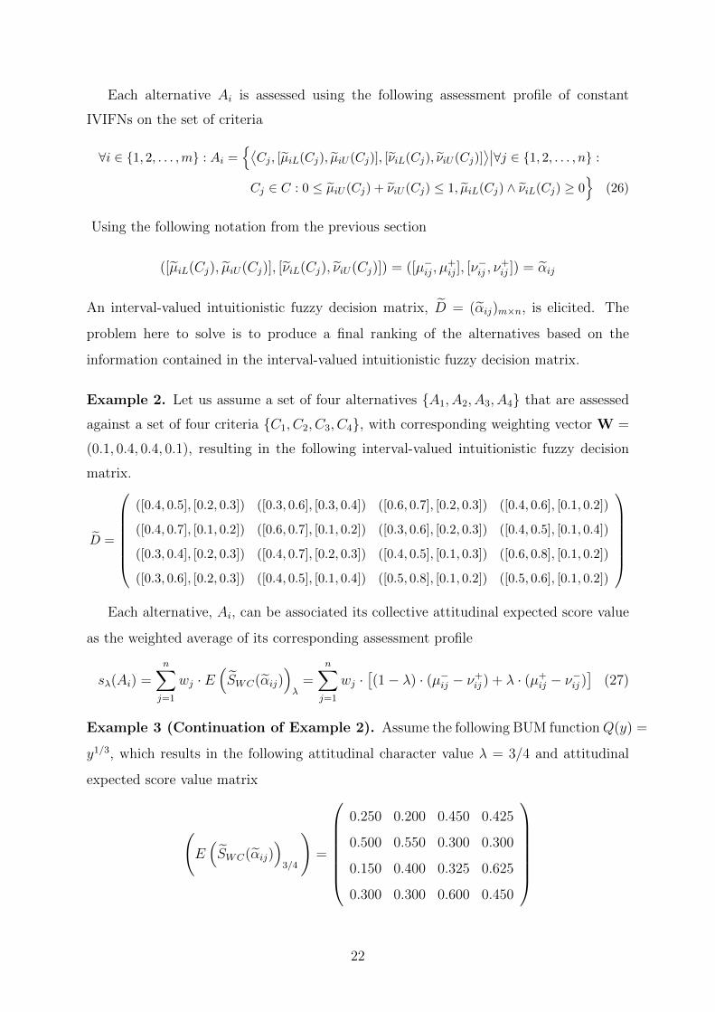
Example 2. Let us assume a set of four alternatives {A1, A2, A3, A4} that are assessed

against a set of four criteria {C1, C2, C3, C4}, with corresponding weighting vector W =

(0.1, 0.4, 0.4, 0.1), resulting in the following interval-valued intuitionistic fuzzy decision

matrix.

D =

([0.4, 0.5], [0.2, 0.3]) ([0.3, 0.6], [0.3, 0.4]) ([0.6, 0.7], [0.2, 0.3]) ([0.4, 0.6], [0.1, 0.2])

([0.4, 0.7], [0.1, 0.2]) ([0.6, 0.7], [0.1, 0.2]) ([0.3, 0.6], [0.2, 0.3]) ([0.4, 0.5], [0.1, 0.4])

([0.3, 0.4], [0.2, 0.3]) ([0.4, 0.7], [0.2, 0.3]) ([0.4, 0.5], [0.1, 0.3]) ([0.6, 0.8], [0.1, 0.2])

([0.3, 0.6], [0.2, 0.3]) ([0.4, 0.5], [0.1, 0.4]) ([0.5, 0.8], [0.1, 0.2]) ([0.5, 0.6], [0.1, 0.2])

Each alternative, Ai, can be associated its collective attitudinal expected score value

as the weighted average of its corresponding assessment profile

sλ(Ai) =n∑j=1

wj · E(SWC(αij)

)λ

=n∑j=1

wj ·[(1− λ) · (µ−

ij − ν+ij ) + λ · (µ+

ij − ν−ij )]

(27)

Example 3 (Continuation of Example 2). Assume the following BUM functionQ(y) =

y1/3, which results in the following attitudinal character value λ = 3/4 and attitudinal

expected score value matrix

(E(SWC(αij)

)3/4

)=

0.250 0.200 0.450 0.425

0.500 0.550 0.300 0.300

0.150 0.400 0.325 0.625

0.300 0.300 0.600 0.450

22

The collective attitudinal expected score values are:

s3/4(A1) = 0.3275, s3/4(A2) = 0.42, s3/4(A3) = 0.3675, s3/4(A4) = 0.510.

The final ranking of the alternatives would be:

A4 � A2 � A3 � A1.

The ranking of the alternatives depends on the value chosen for the attitudinal pa-

rameter λ, and therefore it would be interesting to know the conditions under which a

change in the attitudinal value does not result in a reverse ordering of two alternatives.

These conditions are given in the following sensitivity analysis theorem of the collective

attitudinal expected score value (27).

Theorem 4. Let λ be an attitudinal parameter value under which it has been established

that sλ(Ak) ≤ sλ(Al). Let ∆λ be a perturbation of the attitudinal character λ with

0 ≤ λ+ ∆λ ≤ 1. Then we have

sλ+∆λ(Ak) ≤ sλ+∆λ(Al)

iff

max

{− λ, sλ(Al)− sλ(Ak)

θk − θl

}≤ ∆λ ≤ 1− λ, if θk < θl

−λ ≤ ∆λ ≤ 1− λ, if θk = θl

−λ ≤ ∆λ ≤ min

{1− λ, sλ(Al)− sλ(Ak)

θk − θl

}, if θk > θl

where θk =∑n

j=1wj ·(µ+kj − µ

−kj + ν+

kj − ν−kj

)and θl =

∑nj=1 wj ·

(µ+lj − µ

−lj + ν+

lj − ν−lj

).

Proof. Notice that ∆λ is subject to the following constraint:

−λ ≤ ∆λ ≤ 1− λ.

We have the following relation between sλ+∆λ(Ak) and sλ(Ak):

sλ+∆λ(Ak) = sλ(Ak) + ∆λ · θk, with θk =n∑j=1

wj ·(µ+kj − µ

−kj + ν+

kj − ν−kj

).

The following equivalence holds:

sλ+∆λ(Ak) ≤ sλ+∆λ(Al)⇔ ∆λ · (θk − θl) ≤ sλ(Al)− sλ(Ak). (28)

Three scenarios are possible:

23

• θk = θl. Because sλ(Ak) ≤ sλ(Al) then (28) is true for any value of ∆λ, i.e.

−λ ≤ ∆λ ≤ 1− λ.

• θk > θl ⇔ ∆λ ≤ sλ(Al)− sλ(Ak)θk − θl

, and therefore:

−λ ≤ ∆λ ≤ min

{1− λ, sλ(Al)− sλ(Ak)

θk − θl

}.

• θk < θl ⇔ ∆λ ≥ sλ(Al)− sλ(Ak)θk − θl

, and therefore:

max

{− λ, sλ(Al)− sλ(Ak)

θk − θl

}≤ ∆λ ≤ 1− λ.

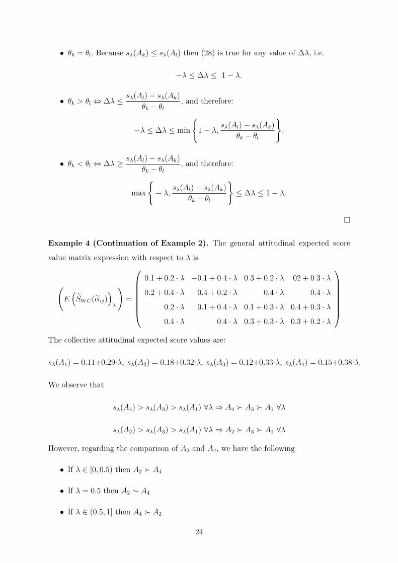
Example 4 (Continuation of Example 2). The general attitudinal expected score

value matrix expression with respect to λ is

(E(SWC(αij)

)λ

)=

0.1 + 0.2 · λ −0.1 + 0.4 · λ 0.3 + 0.2 · λ 02 + 0.3 · λ

0.2 + 0.4 · λ 0.4 + 0.2 · λ 0.4 · λ 0.4 · λ

0.2 · λ 0.1 + 0.4 · λ 0.1 + 0.3 · λ 0.4 + 0.3 · λ

0.4 · λ 0.4 · λ 0.3 + 0.3 · λ 0.3 + 0.2 · λ

The collective attitudinal expected score values are:

sλ(A1) = 0.11+0.29·λ, sλ(A2) = 0.18+0.32·λ, sλ(A3) = 0.12+0.33·λ, sλ(A4) = 0.15+0.38·λ.

We observe that

sλ(A4) > sλ(A3) > sλ(A1) ∀λ⇒ A4 � A3 � A1 ∀λ

sλ(A2) > sλ(A3) > sλ(A1) ∀λ⇒ A2 � A3 � A1 ∀λ

However, regarding the comparison of A2 and A4, we have the following

• If λ ∈ [0, 0.5) then A2 � A4

• If λ = 0.5 then A2 ∼ A4

• If λ ∈ (0.5, 1] then A4 � A2

24

Summarising, we have the following:

• ∀ λ ∈ [0, 0.5) we have: A2 � A4 � A3 � A1.

• If λ = 0.5 then A2 ∼ A4 � A3 � A1.

• ∀λ ∈ (0.5, 1] we have: A4 � A2 � A3 � A1.

Therefore only when the value of λ is close to 0.5, we may have a reversal ordering of

the alternatives A2 and A4. It is worth remarking here that the final ordering of the

alternatives not only depends on the value of the attitudinal character but also on the

particular criteria weighting vector, an issue that will be the focus of future research

work.

The collective attitudinal expected score values results in a total ordering of the

set of alternatives. For those alternatives with same collective attitudinal expected score

values, we apply the second level ordering with the application of the collective attitudinal

accuracy score value

aλ(Ai) =n∑j=1

wj · E(AWC(αij)

)λ

=n∑j=1

wj ·[(1− λ) · (µ−

ij + ν−ij ) + λ · (µ+ij + ν+

ij )]

(29)

An alternative expression to (29) for the collective attitudinal accuracy score value can

be obtained if the relationship (20) between the the attitudinal expected accuracy score

function and the attitudinal expected accuracy function is used:

aλ(Ai) =n∑j=1

wj · E(AWC(αij)

)λ

=n∑j=1

wj ·[E(SWC(αij)

)λ

+ (ν+ij + ν−ij )

]=sλ(Ai) +

n∑j=1

wj · (ν+ij + ν−ij ). (30)

Example 5 (Continuation of Example 2). In Example 4, we had s0.5(A2) = s0.5(A2) =

0.34. It is easy to prove that in this case we have that a0.5(A2) = a0.5(A2) = 0.74, so

we can not decide yet which alternative is the best. To do that, we apply the third level

ordering based on the use of the membership uncertainty index. Obviously, a different

criteria weighting vector to the one used in these examples might have led to different

attitudinal expected accuracy values.

A similar reasoning to that of Theorem 4 can be used to prove the following sensitivity

analysis of the collective attitudinal expected accuracy value (27):

25

Theorem 5. Let λ be an attitudinal parameter value under which it has been established

that aλ(Ak) ≤ aλ(Al). Let ∆λ be a perturbation of the attitudinal character λ with

0 ≤ λ+ ∆λ ≤ 1. Then we have

aλ+∆λ(Ak) ≤ aλ+∆λ(Al)

iff

max

{− λ, aλ(Al)− aλ(Ak)

θk − θl

}≤ ∆λ ≤ 1− λ, if θk < θl

−λ ≤ ∆λ ≤ 1− λ, if θk = θl

−λ ≤ ∆λ ≤ min

{1− λ, aλ(Al)− aλ(Ak)

θk − θl

}, if θk > θl

where θk =∑n

j=1wj ·(µ+kj − µ

−kj + ν+

kj − ν−kj

)and θl =

∑nj=1 wj ·

(µ+lj − µ

−lj + ν+

lj − ν−lj

).

For those alternatives with same collective attitudinal expected score values and col-

lective attitudinal accuracy score value, we apply the third level ordering with the com-

putation of their respective collective membership uncertainty indexes.

T (Ai) =n∑j=1

wj ·[(µ+ij − µ−

ij

)−(ν+ij − ν−ij

)]. (31)

Example 6 (Finishing Example 2). The collective membership uncertainty indexes

corresponding to alternatives A2 and A4 are T (A2) = −0.04 and T (A4) = 0.04, and

therefore the final ranking of the set of alternatives when λ = 0.5 would be:

A2 � A4 � A3 � A1.

5. Conclusion

Based on the concept of attitudinal character of a BUM and the continuous ordered

weighted average (COWA) operator, attitudinal expected score and accuracy functions

for IVIFNs are introduced and their relationship with existing score and accuracy degree

functions are investigated. A set of properties are also proved, which makes them to be

a type of weighted average operators. A key result provided is the construction of a total

order on the set of IVIFNs using a three level ordering relation based on the conjunction

application of the attitudinal expected score and accuracy functions and Wang et al.’s

membership uncertainty index function. A resolution process of interval-valued intuition-

istic fuzzy multi-attribute decision making problems that ranks the alternatives by taking

26

accounting of the decision makers’ risk attitude is also provided. It was remarked before

that the final ordering of the alternatives not only depends on the value of the attitudinal

character but also on the particular criteria weighting vector, which in conjunction with

the development of consistency based decision models [47] will be the focus of future

research work.

Acknowledgements

The authors are very grateful to the anonymous referees for their comments and sug-

gestions. This work was supported by National Natural Science Foundation of China

(NSFC) under the Grant No.71101131 and Zhejiang Provincial National Science Foun-

dation for Distinguished Young Scholars of China under the Grant No. LR13G010001.

[1] K. Atanassov, Intuitionistic fuzzy sets, Fuzzy Sets and Systems 20 (1986), 87–96.

[2] L. A. Zadeh, Fuzzy sets, Information and Control 8 (1965), 338–353.

[3] J. Wu, F. Chiclana: A social network analysis trust-consensus based approach to

group decision-making problems with interval-valued fuzzy reciprocal preference re-

lations, Knowledge-Based Systems 59 (2014), 97–107.

[4] K. Atanassov and G. Gargov, Interval-valued intuitionistic fuzzy sets, Fuzzy Sets

and Systems 31 (1989), 343–349.

[5] Z. J. Wang, K. W. Li and J. H. Xu, A mathematical programming approach to

multi-attribute decision making with interval-valued intuitionistic fuzzy assessment

information, Expert Systems with Applications 38 (2011), 12462–12469.

[6] Y. J. Yang and F. Chiclana, Intuitionistic fuzzy sets: Spherical representation and

distances, International Journal of Intelligent Systems 24 (2009), 399–420.

[7] Y. J. Yang and F. Chiclana,, Consistency of 2D and 3D distances of intuitionistic

fuzzy sets, Expert Systems with Applications 39 (2012), 8665–8670.

[8] J. Wu and F. Chiclana, Non-dominance prioritization methods for intuitionistic and

interval-valued intuitionistic preference relations, Expert Systems with Applications

39 (2012), 13409–13416

27

[9] J. Wu, H.B.Huang and Q.W.Cao, Research on AHP with interval-valued intuitionis-

tic fuzzy sets and its application in multi-criteria decision making problems, Applied

Mathematical Modelling 37 (2013), 9898–9906

[10] J. Wu and Y.J. Liu, An approach for multiple attribute group decision making

problems with interval-valued intuitionistic trapezoidal fuzzy numbers, Computers

and Industrial Engineering 66(2013), 311–324

[11] T. Y. Chen, Multiple criteria group decision-making with generalized interval-valued

fuzzy numbers based on signed distances and incomplete weights, Applied Mathema-

tical Modelling 36 (2012), 3029–3052.

[12] Z. L. Yue, An approach to aggregating interval numbers into interval-valued intu-

itionistic fuzzy information for group decision making, Expert Systems with Applica-

tions 38 (2011), 6333–6338.

[13] F. Ye, An extended TOPSIS method with interval-valued intuitionistic fuzzy num-

bers for virtual enterprise partner selection, Expert Systems with Applications 37

(2010), 7050–7055.

[14] J. Ashayeri, G. Tuzkaya and U. R. Tuzkaya, Supply chain partners and configuration

selection: An intuitionistic fuzzy Choquet integral operator based approach, Expert

Systems with Applications 39 (2012), 3642–3649.

[15] K.Devi, Extension of VIKOR method in intuitionistic fuzzy environment for robot

selection, Expert Systems with Applications 38 (2011), 14163–14168.

[16] R. Saadati, S. M. Vaezpour and Y. J. Choc, Quicksort algorithm: Application of a

fixed point theorem in intuitionistic fuzzy quasi-metric spaces at a domain of words,

Journal of Computational and Applied Mathematics 228 (2009), 219–225.

[17] F. Chiclana, E. Herrera-Viedma, F. Herrera, S. Alonso: Some induced ordered

weighted averaging operators and their use for solving group decision-making prob-

lems based on fuzzy preference relations, European Journal of Operational Research

182 (1) (2007), 383–399.

[18] Z. S. Xu, Intuitionistic fuzzy aggregation operators, IEEE Transactions on Fuzzy

Systems 15 (2007), 1179–1187.

28

[19] D. F. Li, The GOWA operator based approach to multiattribute decision making

using intuitionistic fuzzy sets, Mathematical and Computer Modelling 53 (2011),

1182–1196.

[20] Z. S. Xu, Methods for aggregating interval-valued intuitionistic fuzzy information

and their application to decision making, Control and Decision 22 (2007), 215–219.

[21] J. Wu and Q. W. Cao, Same families of geometric aggregation operators with in-

tuitionistic trapezoidal fuzzy numbers, Applied Mathematical Modelling 37 (2013),

318–327.

[22] C. Q. Tan and X. H. Chen, Intuitionistic fuzzy Choquet integral operator for multi-

criteria decision making, Expert Systems with Applications 37 (2010), 149–157.

[23] C. Q. Tan, A multi-criteria interval-valued intuitionistic fuzzy group decision making

with Choquet integral-based TOPSIS, Expert Systems with Applications 38 (2011),

3023–3033.

[24] T. Y. Chen, A comparative analysis of score functions for multiple criteria decision

making in intuitionistic fuzzy settings, Information Sciences 181 (2011), 3652–3676.

[25] S. M. Chen and J. M. Tan, Handling multi-criteria fuzzy decision-making problems

based on vague set theory, Fuzzy Sets and Systems 67 (1994), 163–172.

[26] D. H. Hong and C.H. Choi, Multicriteria fuzzy decision-making problems based on

vague set theory, Fuzzy Sets and Systems 114 (2000), 103–113.

[27] J. Q. Wang, L. Y. Meng and X. H. Cheng, Multi-criteria decision making method

based on vague sets and risk attitudes of decision makers, Systems Engineering and

Electronics 2 (2009), 361–365.

[28] K. Atanassov, G. Pasi and R. R. Yager, Intuitionistic fuzzy interpretations of multi-

criteria multi-person and multi-measurement tool decision making, International

Journal of Systems Science 36 (2005), 859–868.

[29] T. Y. Chen, An outcome-oriented approach to multicriteria decision analysis with in-

tuitionistic fuzzy optimistic/pessimistic operators, Expert Systems with Applications

37 (2010), 7762–7774.

29

[30] S. P. Wan, and J. Y. Dong, A possibility degree method for interval-valued intuition-

istic fuzzy multi-attribute group decision making, Journal of Computer and System

Sciences 80 (2014), 237–256.

[31] Z. J. Wang, K. W. Li and W. Wang, An approach to multiattribute decision making

with interval-valued intuitionistic fuzzy assessments and incomplete weights, Infor-

mation Sciences 179 (2009), 3026–3040.

[32] J. Q. Wang, K. J. Li and H. Y. Zhang, Interval-valued intuitionistic fuzzy multi-

criteria decision-making approach based on prospect score function, Knowledge-

Based Systems 27 (2012), 119–215.

[33] S. P. Wan, Q. Y. Wang, and J. Y. Dong, The extended VIKOR method for multi-

attribute group decision making with triangular intuitionistic fuzzy numbers, Knowl-

edge Based Systems 52 (2013), 65–77.

[34] S. P. Wan, Multi-attribute decision making method based on possibility variance

coefficient of triangular intuitionistic fuzzy numbers, International Journal of Un-

certainty, Fuzziness and Knowledge-Based Systems 21 (2014), 223–243.

[35] P.D. Liu, and J. Y. Dong, Methods for Aggregating Intuitionistic Uncertain Linguis-

tic variables and Their Application to Group Decision Making, Information Sciences

205(2012), 58–71.

[36] P.D. Liu, Some Generalized Dependent Aggregation Operators with Intuitionistic

Linguistic Numbers and Their Application to Group Decision Making, Journal of

Computer and System Sciences 79(2013), 131–143.

[37] P.D. Liu, and Y. M. Wang, Multiple Attribute Group Decision Making Methods

Based on Intuitionistic Linguistic Power Generalized Aggregation Operators, Applied

soft computing 17(2014), 90–104.

[38] Z. S. Xu and J. Chen, An approach to group decision making based on interval-valued

intuitionistic judgment matrices, System Engineer-Theory & Practice 27 (2007), 126–

133.

30

[39] J. Ye, Multicriteria fuzzy decision-making method based on a novel accuracy function

under interval-valued intuitionistic fuzzy environment, Expert Systems with Appli-

cations 36 (2009), 6899–6902.

[40] V. Lakshmana Gomathi Nayagama and G. Sivaraman, Ranking of interval-valued

intuitionistic fuzzy sets, Applied Soft Computing 11 (2011), 3368–3372.

[41] R. R. Yager, OWA aggregation over a continuous interval argument with applications

to decision making, IEEE Transactions on Systems, Man, and Cybernetics-Part B:

Cybernetics 34 (2004), 1952–1963.

[42] M. Hanss, Applied Fuzzy Arithmetic. An Introduction with Engineering Applica-

tions. Springer-Verlag Berlin Heidelberg, 2005.

[43] P. Perez-Asurmendi, F. Chiclana. Linguistic majorities with difference in support.

Applied Soft Computing, 18 (2014) 196–208.

[44] L.A. Zadeh. Outline of a new approach to the analysis of complex systems and

decision processes, IEEE Transactions on Systems, Man and Cybernetics, 3, 28–44,

1973.

[45] M. Brunelli, J. Mezei. How different are ranking methods for fuzzy numbers? A

numerical study, International Journal of Approximate Reasoning, 54 (5), 627–639,

2013.

[46] R. Yager. Quantifier guided aggregation using owa operators. International Journal

of Intelligent Systems 11 (1), 1996, 49–73.

[47] F. Chiclana, E. Herrera-Viedma, S. Alonso, F. Herrera: Cardinal consistency of

reciprocal preference relations: a characterization of multiplicative transitivity. IEEE

Transactions on Fuzzy Systems 17 (1) (2009), 14–23.

31