Embed Size (px)
Citation preview

A Review onSCARA Robotic Arm
Supervisor:Dr. Rahbari Asr
Presented By:Farid , Alidoust1
Mojtaba , Alizadeh2
1- [email protected]@alidoost.ir2- [email protected] [email protected] M
ech
atro
nic
Dep
artm
ent
Isla
mic
Aza
d U
niv
ersi
ty ,
Tab
riz
Bra
nch

Topics

Introduction
Why Industrial Robotic Arms ?
A general-purpose, programmable machine possessing certain anthropomorphic characteristics
Used in: Hazardous work environments Repetitive work cycle Consistency and accuracy
needed! Difficult handling task for
humans Multi-shift operations for
industries Reprogrammable, flexible Interfaced to other computer
systems

Introduction
In 1981, Sankyo Seiki, Pentel and NEC presented a completely new concept for assembly robots.
The robot was developed under the guidance of Hiroshi Makino, a professor at the University of Yamanashi.
Its arm was rigid in the Z-axis and pliable in the XY-axes, which allowed it to adapt to holes in the XY-axes.

Introduction
Notation VRO.SCARA stands for
Selectively Compliant Assembly Robot Arm.
Similar to jointed-arm robot except that vertical axes are used for shoulder and elbow joints to be compliant in horizontal direction for vertical insertion tasks.

The Scara Properties
Developed to meet the needs of modern assembly.
Fast movement with light payloads
Rapid placements of electronic components on PCB’s
Combination of two horizontal rotational axes and one linear joint.

Kinematic of Operation

Denavit–Hartenberg co-ordinates
Jaques Denavit and Richard S. Hartenberg presented the first minimal representation for a line which is now widely used.
Engineers use the Denavit–Hartenberg convention (D–H) to help them describe the positions of links and joints unambiguously.

Denavit–Hartenberg Line co-ordinates
Every link gets its own coordinate system. There are a few rules to consider in choosing the coordinate system:
1.the z-axis is in the direction of the joint axis2.the x-axis is parallel to the common normal:
If there is no unique common normal (parallel z axes), then d (below) is a free parameter.
3.the y-axis follows from the x- and z-axis by choosing it to be a right-handed coordinate system.

Denavit–Hartenberg Line co-ordinates
Once the coordinate frames are determined, inter-link transformations are uniquely described by the following four parameters:
: angle about previous z, from old x to new x : offset along previous z to the common
normal : length of the common normal (aka a, but if
using this notation, do not confuse with α). Assuming a revolute joint, this is the radius about previous z.
: angle about common normal, from old z axis to new z axis
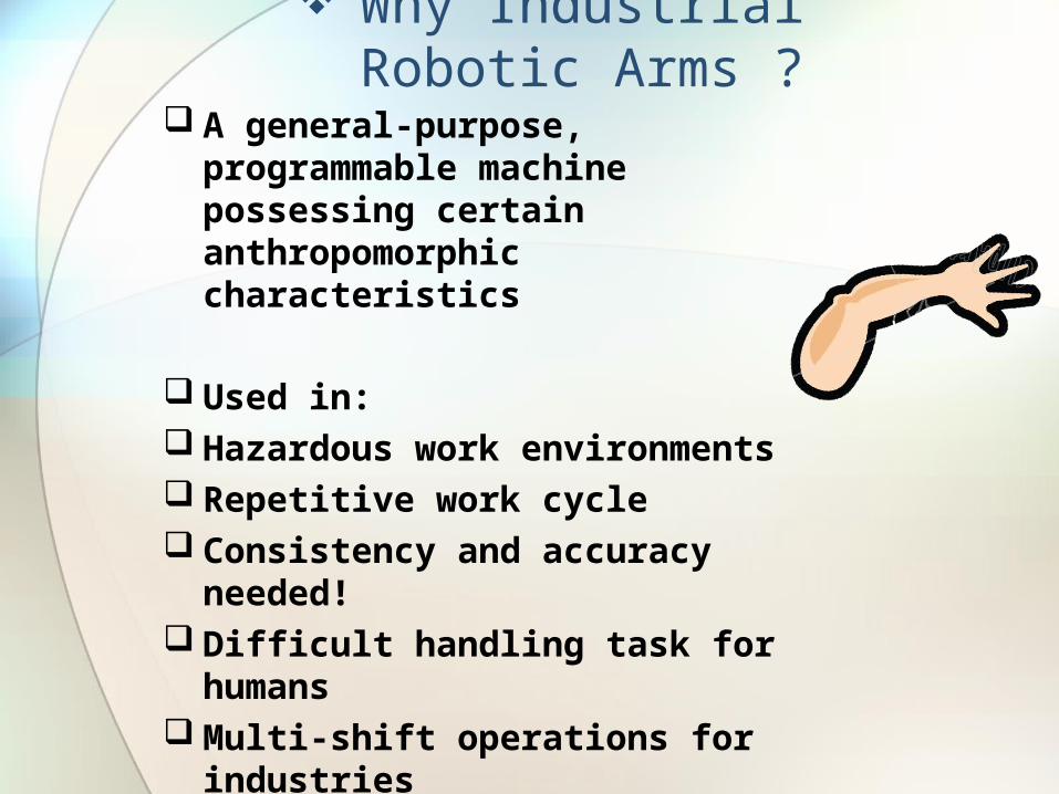
Use the DH Algorithm to assign the frames and kinematic parameters
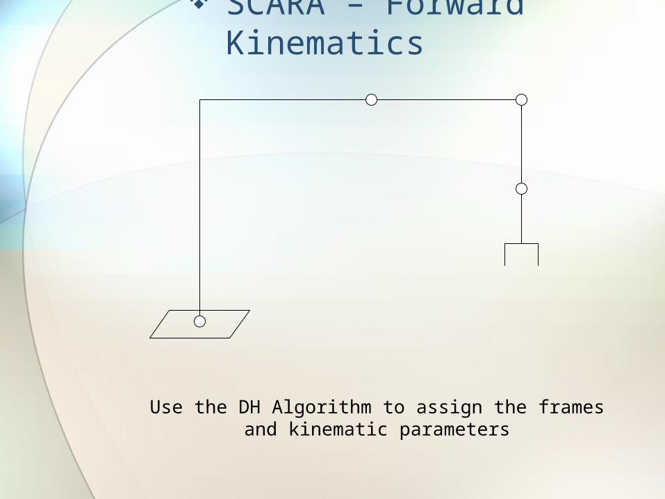
SCARA – Forward Kinematics
Number the joints 1 to n starting with the base and ending with the tool yaw, pitch and roll in that order.
Note: There is no tool pitch or yawno tool pitch or yaw in this case
1
2 3
4-Tool Roll

z0 y0
z1
x1y1z2
x2
y2
z3
x3
z4
y3
y4
x4
x0
d4
d3
a2
d1
a1
1
4
2
From this drawing of D-H parameters can be compiled
Full DH-Algorithm presentation attached to appendix in final of presentation

z0 y0
z1
x1y1z2
x2
y2
z3
x3
z4
y3
y4
x4
x0
d4
d3
a2
d1
a1
1
4
2
Joint d a Home q
1 1 d1 a1 180º 0º
2 2 0 a2
0º 0º
3 0º
d3 0 0º dmax
4 4 d4 0
0º 90º

Applications

Applications Useful in Semiconductor Fabrication Industries.
mostly adopted wafer handling robot in semi-conductor industry
A radius layout, for wafer carriers and aligner
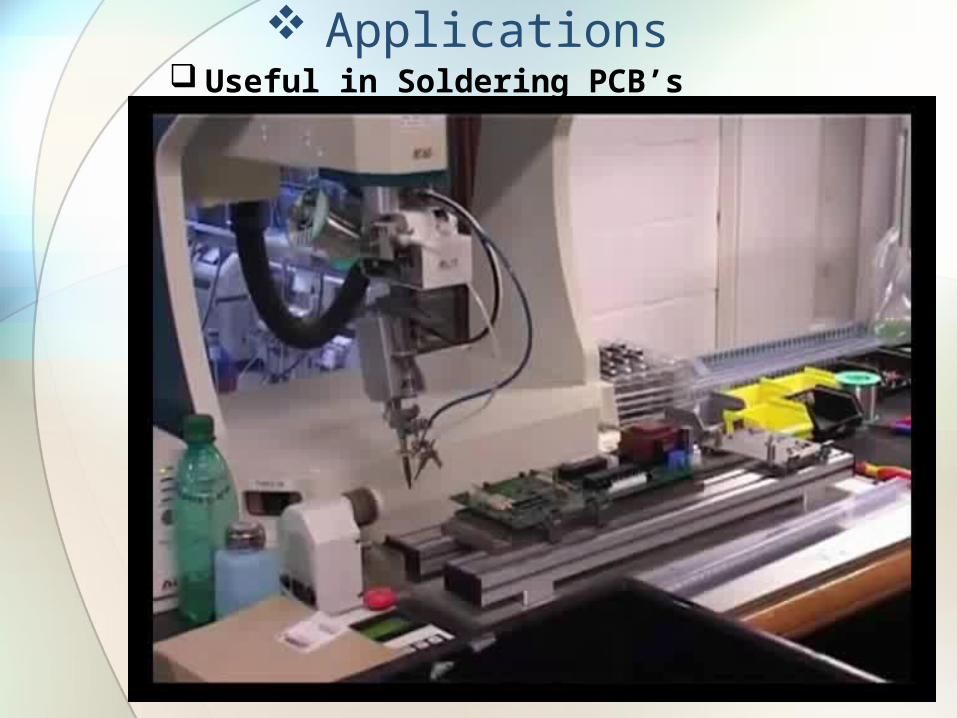
Applications Useful in Soldering PCB’s

Applications Finished product inspection, touch-panel type
evaluation machine
Finished product function test.Developed software evaluation.Push button type quality check.
POINT: Supports a variety of systems in a product line Space saving. Using SCARA, judgment is made throughimage processing by pushing each button.

Applications Pharmaceutical Industries

Applications Part Sortation

Applications Tall work pieces conveying and stacking machine >>
Tall work pieces stacked by utilizing long Z axis.
POINT: Use of SCARA can cope with the Z axis long stroke as
quasi standard. Advantages of use of SCARA: speed of XY axis and
space saving installation.

Applications Assembling (such as Cosmetic Handling and Packaging)

Applications Assembly cell (independent cell) >>
Base machine of independent type assembly cell.
POINT: Optimum for multi type variable quantity
production. Setting up reception places forms a construction of
multiple number of cells.

Applications Assembly cell (independent cell) >>
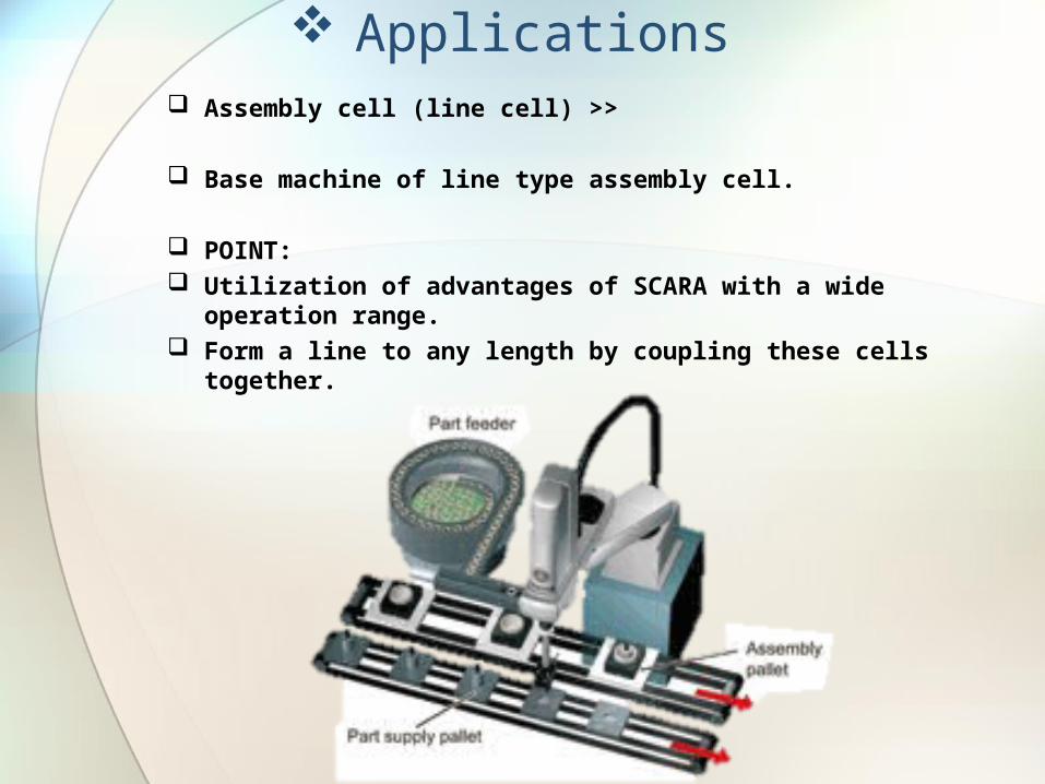
Applications Assembly cell (line cell) >>
Base machine of line type assembly cell.
POINT: Utilization of advantages of SCARA with a wide
operation range. Form a line to any length by coupling these cells
together.

Applications Assembly cell (line cell) >>

Applications Assembly cell (line cell) >>

Manipulators

End Effectors The special tooling for a robot that
enables it to perform a specific task
Two types:
Grippers – to grasp and manipulate objects (e.g., parts) during work cycle
Tools – to perform a process, e.g., spot welding, spray painting
End Effector

Grippers: mechanical, magnetic and pneumatic.
Mechanical: Two finger most common, also multi-
fingered available. Applies force that causes enough friction
between object to allow for it to be lifted.
Not suitable for some objects which may be delicate / brittle
End Effectors

Magnetic:
Ferrous materials required Electro and permanent magnets used
Pneumatic: Suction cups from plastic or rubber Smooth even surface required Weight & size of object determines
size and number of cups
End Effectors

Ladle
Ladling hot materials such as molten metal is a hot and hazardous job for which industrial robots are well suited.
In piston casting permanent mold , die casting and related applications, the robot can be programmed to scoop up and transfer the molten metal from the pot to the mold, and then do the pouring.

Spray gun
Ability of the industrial robot to do multipass spraying with controlled velocity fits it for automated application of primers, paints, and ceramic or glass frits, as well as application of masking agents used before plating.
For short or medium‑length production runs, the industrial robot would often be a better choice than a special purpose setup requiring a lengthy change‑over procedure for each different part.
Also the robot can spray parts with compound curvatures and multiple surfaces.

Tool changing
A single industrial robot can also handle several tools sequentially, with an automatic tool changing operation programmed into the robot's memory.
The tools can be of different types or sizes, permitting multiple operations on the same workpiece.

Servo motors Acts as Actuator
Contain motor, gearbox, driver controller and potentiometer
Three wires - 0v, 5v and signal Potentiometer connected to gearbox –
monitors movement Provides feedback If position is distorted - automatic
correction
+ 5V
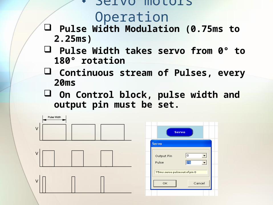
Servo motors Operation Pulse Width Modulation (0.75ms to
2.25ms) Pulse Width takes servo from 0° to 180°
rotation Continuous stream of Pulses, every 20ms On Control block, pulse width and output
pin must be set.

Top Brandsfor SCARA robots:

Fastest SCARA robot in World

Conclusion on SCARA Robots
Advantages: - 1 linear axis, 2 rotating
axes - Height axis is rigid - Large work area floor
space - Can reach around obstacles - Two ways to reach a point
Disadvantages: - Difficult to program off‑line - Highly complex arm
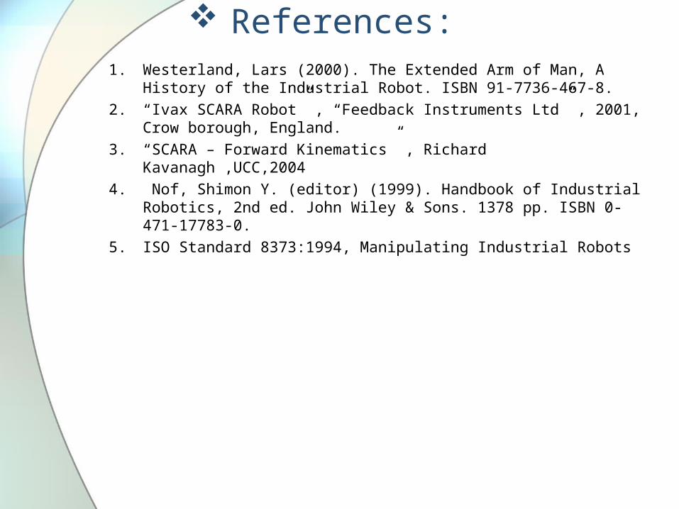
References:1. Westerland, Lars (2000). The Extended Arm of Man, A History of
the Industrial Robot. ISBN 91-7736-467-8.2. “Ivax SCARA Robot” , “Feedback Instruments Ltd” , 2001, Crow
borough, England.3. “SCARA – Forward Kinematics” , Richard Kavanagh ,UCC,20044. Nof, Shimon Y. (editor) (1999). Handbook of Industrial Robotics,
2nd ed. John Wiley & Sons. 1378 pp. ISBN 0-471-17783-0.5. ISO Standard 8373:1994, Manipulating Industrial Robots

Any Questions ?!

Thank for Audience

AppendixFull DH Algorithm
Represent

Assign a right-handed orthonormal frame L0 to the robot base, making sure that z0 aligns with the axis of joint. Set k=1
z0
x0
y0
k=0

z0
x0
y0
z1
2
Align zk with the axis of joint k+1.
Locate the origin of Lk at the intersection of the zk and zk-1axesIf they do not intersect use the the intersection of zk with a common normal between zk and zk-1.(can point up or down in this case)
Common Normal
k=1

z0
x0
y0
z1
Select xk to be orthogonal to both zk and zk-1.
If zk and zk-1are parallel, point xk away from zk-1.
Select yk to form a right handed orthonormal co-ordinate frame Lk
x1y1
k=1

z0 y0
z1
x1y1
Align zk with the axis of joint k+1.
Vertical Extension
Again zk and zk-1 are parallel the so we use the intersection of zk
with a common normal.
Common Normal
z2
x0
k=2

z0 y0
z1
x1y1
z2
Select xk to be orthogonal to both zk and zk-1.
Once again zk and zk-1are parallel, point xk away from zk-1.
x2
y2
Select yk to complete the right handed orthonormal co-ordinate frame
x0
k=2

z0 y0
z1
x1y1z2
x2
y2
Align zk with the axis of joint k+1.
4
Locate the origin of Lk at the intersection of the zk and zk-1axes
z3
x0
k=3

z0 y0
z1
x1y1z2
x2
y2
z3
Select xk to be orthogonal to both zk and zk-1.
Again xk can point in either direction. It is chosen to point in the same direction as xk-1
x3
Select yk to complete the right handed orthonormal co-ordinate frame
y3
x0
k=3

z0 y0
z1
x1y1z2
x2
y2
z3
x3
Set the origin of Ln at the tool tip. Align zn with the approach vector of the tool.
z4
Align yn with the sliding vector of the tool.
y3
y4
Align xn with the normal vector of the tool.
x4
x0
k=4

z0 y0
z1
x1y1z2
x2
y2
z3
x3
z4
y3
y4
x4
x0
With the frames assigned the kinematic parameters can be determined.

z0 y0
z1
x1y1z2
x2
y2
z3
x3
z4
y3
y4
x4
x0
Locate point bk at the intersection of the xk and zk-1 axes. If they do not intersect, use the intersection of xk with a common normal
between xk and zk-1
b4
k=4

z0 y0
z1
x1y1z2
x2
y2
z3
x3
z4
y3
y4
x4
x0
Compute k as the angle of rotation from xk-1 to xk measured about zk-1
It can be seen here that the angle of rotation from xk-1 to xk about zk-1 is 90 degrees (clockwise +ve) i.e. 4 = 90º
But this is only for the soft home position, 4 is the joint variable.
4
k=4
z0 y0
z1
x1y1z2
x2
y2
z3
x3
z4
y3
y4
x4
x0
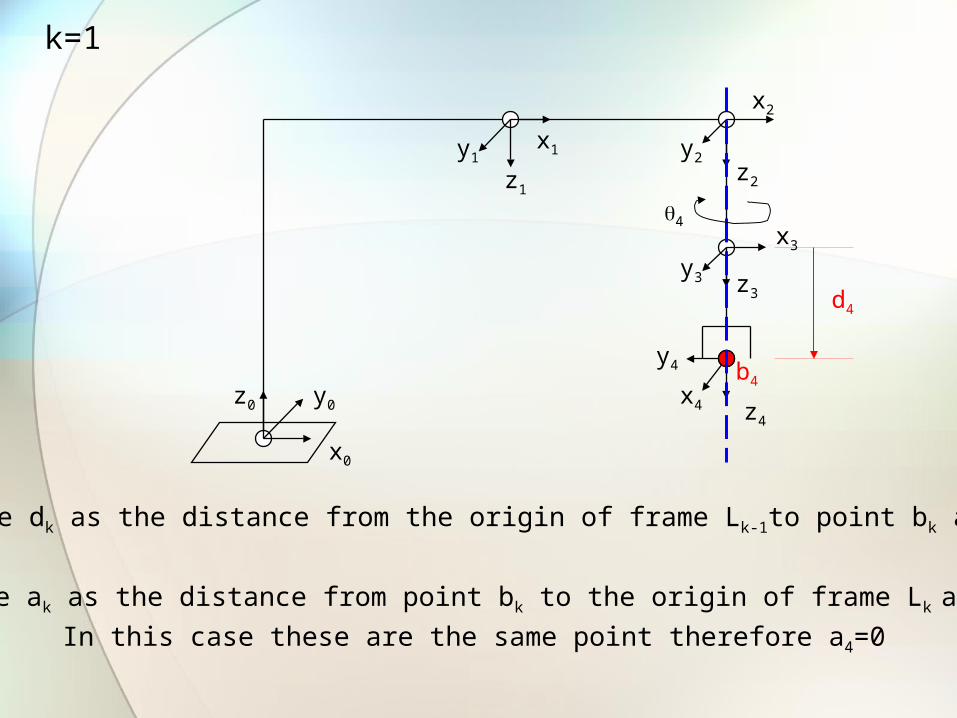
Compute dk as the distance from the origin of frame Lk-1to point bk along zk-1
b4
d4
Compute ak as the distance from point bk to the origin of frame Lk along xk
In this case these are the same point therefore a4=0
4
k=1
z0 y0
z1
x1y1z2
x2
y2
z3
x3
z4
y3
y4
x4
x0
b4
d4
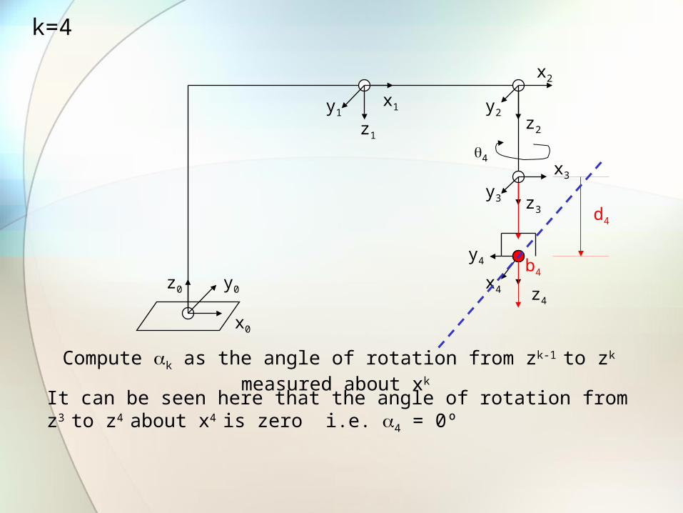
Compute k as the angle of rotation from zk-1 to zk measured about xk
It can be seen here that the angle of rotation from z3 to z4 about x4 is zero i.e. 4 = 0º
4
k=4
z0 y0
z1
x1y1z2
x2
y2
z3
x3
z4
y3
y4
x4
x0
b3
d4
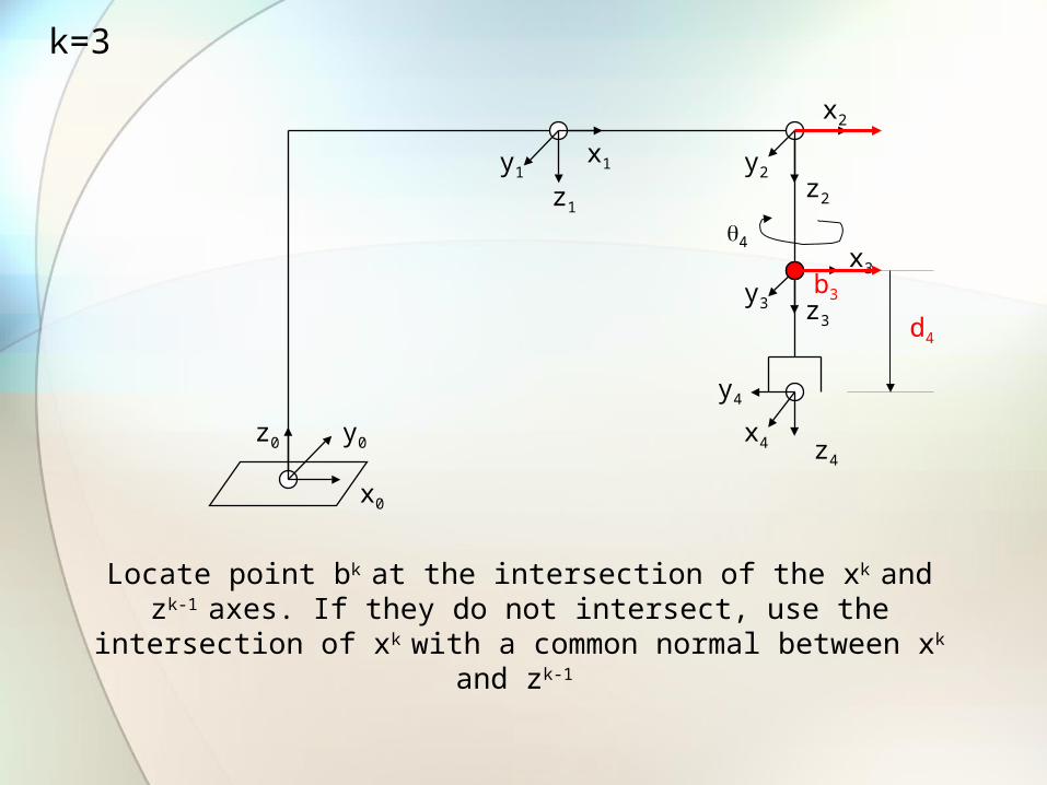
Locate point bk at the intersection of the xk and zk-1 axes. If they do not intersect, use the intersection of xk with a common normal
between xk and zk-1
4
k=3

z0 y0
z1
x1y1z2
x2
y2
z3
x3
z4
y3
y4
x4
x0
b3
d4
Compute k as the angle of rotation from xk-1 to xk measured about zk-1
It can be seen here that the angle of rotation from xk-1 to xk about zk-1 is zero i.e. 3 = 0º
4
k=3

z0 y0
z1
x1y1z2
x2
y2
z3
x3
z4
y3
y4
x4
x0
b3
d4
Compute dk as the distance from the origin of frame Lk-1to point bk along zk-1
Compute ak as the distance from point bk to the origin of frame Lk along xk
In this case these are the same point, therefore ak=0
d3
Since joint 3 is prismatic d3 is the joint variable
4
k=3

z0 y0
z1
x1y1z2
x2
y2
z3
x3
z4
y3
y4
x4
x0
b3
d4
d3
Compute k as the angle of rotation from zk-1 to zk measured about xk
It can be seen here that the angle of rotation from z2 to z3 about x3 is zero i.e. 3 = 0º
4
k=3

z0 y0
z1
x1y1z2
x2
y2
z3
x3
z4
y3
y4
x4
x0
b2
d4
d3
Once again locate point bk at the intersection of the xk and zk-1 axes If they did not intersect we would use the intersection of xk with a
common normal between xk and zk-1
4
k=2

z0 y0
z1
x1y1z2
x2
y2
z3
x3
z4
y3
y4
x4
x0
b2
d4
d3
Compute k as the angle of rotation from xk-1 to xk measured about zk-1
It can be seen here that the angle of rotation from x1 to x2 about z1 is zero i.e. 2 = 0º
But this is only for the soft home position, 4 is the joint variable.
4
2
k=2
z0 y0
z1
x1y1z2
x2
y2
z3
x3
z4
y3
y4
x4
x0
b2
d4
d3
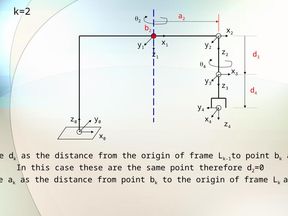
Compute dk as the distance from the origin of frame Lk-1to point bk along zk-1
In this case these are the same point therefore d2=0
Compute ak as the distance from point bk to the origin of frame Lk along xk
a2
4
2
k=2

z0 y0
z1
x1y1z2
x2
y2
z3
x3
z4
y3
y4
x4
x0
b2
d4
d3
a2
Compute k as the angle of rotation from zk-1 to zk measured about xk
It can be seen here that the angle of rotation from z1 to z2 about x2 is zero i.e. 2 = 0º
4
2
k=2

z0 y0
z1
x1y1z2
x2
y2
z3
x3
z4
y3
y4
x4
x0
b1
d4
d3
a2
For the final time locate point bk at the intersection of the xk and zk-1
axes
4
2
k=1

z0 y0
z1
x1y1z2
x2
y2
z3
x3
z4
y3
y4
x4
x0
bk
d4
d3
a2
Compute k as the angle of rotation from xk-1 to xk measured about zk-1
It can be seen here that the angle of rotation from x0 to x1 about z0 is zero i.e. 1 = 0º
But this is only for the soft home position, 1is the joint variable.
1
4
2
k=1

z0 y0
z1
x1y1z2
x2
y2
z3
x3
z4
y3
y4
x4
x0
b1
d4
d3
a2
Compute dk as the distance from the origin of frame Lk-1to point bk along zk-1
Compute ak as the distance from point bk to the origin of frame Lk along xk
d1
a1
1
4
2
k=1

z0 y0
z1
x1y1z2
x2
y2
z3
x3
z4
y3
y4
x4
x0
b1
d4
d3
a2
d1
a1
Compute k as the angle of rotation from zk-1 to zk measured about xk-1
It can be seen here that the angle of rotation from z0 to z1 about x1 is 180 degrees
1
4
2
k=1