A Review of Sequences and Inﬁnite Seriespeople.uncw.edu/hermanr/phy311/MathPhysBook/Series.pdfA Review of Sequences and Inﬁnite Series “Once you eliminate the impossible, whatever

AReview of Sequences and Infinite Series

“Once you eliminate the impossible, whatever remains, no matter how improbable, must be the truth.” Sherlock Holmes(by Sir Arthur Conan Doyle, 1859-1930)

The material in this chapter is a reviewof material covered in a standard coursein calculus with some additional notionsfrom advanced calculus. It is providedas a review before encountering the no-tion of Fourier series and their conver-gence as seen in the next chapter.

In this chapter we will review and extend some of the conceptsand definitions related to infinite series that you might have seen pre-viously in your calculus class (1, 2, 3). Working with infinite series can

1

2

3

be a little tricky and we need to understand some of the basics beforemoving on to the study of series of trigonometric functions in the nextchapter.

As we will see, ln(1 + x) = x− x2 + x

3 −. . . . So, inserting x = 1 yields the firstresult - at least formally! It was shown inCowen, Davidson and Kaufman (in TheAmerican Mathematical Monthly, Vol. 87,No. 10. (Dec., 1980), pp. 817-819) thatexpressions like

f (x) =12

[ln

1 + x1− x

+ ln(1− x4)

]=

12

ln[(1 + x)2(1 + x2)

]lead to alternate sums of the rearrange-ment of the alternating harmonic series.

For example, one can show that the infinite series

S = 1− 12+

13− 1

4+

15− · · ·

converges to ln 2. However, the terms can be rearranged to give

1 +(

13− 1

2+

15

)+

(17− 1

4+

19

)+

(111− 1

6+

113

)+ · · · = 3

2ln 2.

In fact, other rearrangements can be made to give any desired sum!Other problems with infinite series can occur. Try to sum the fol-

lowing infinite series to find that

∞

∑k=2

ln kk2 ∼ 0.937548 . . . .

A sum of even as many as 107 terms only gives convergence to four orfive decimal places.

The series1x− 1

x2 +2!x3 −

3!x4 +

4!x5 − · · · , x > 0

diverges for all x. So, you might think this divergent series is useless.However, truncation of this divergent series leads to an approximationof the integral ∫ ∞

0

e−t

x + tdt, x > 0.

466 mathematical physics

So, can we make sense out of any of these, or other manipulations,of infinite series? We will not answer these questions now, but we willgo back and review what you have seen in your calculus classes.

A.1 Sequences of Real Numbers

We first begin with the definitions for sequences and series of num-bers.

Definition A.1. A sequence is a function whose domain is the set ofpositive integers, a(n), n ∈ N [N = {1, 2, . . . .}].

2 4 6 8 10

0

2

4

6

8

n

Plot of an = n− 1 vs n

Figure A.1: Plot of an = n − 1 for n =1 . . . 10.

Examples are

1. a(n) = n yields the sequence {1, 2, 3, 4, 5, . . .}

2. a(n) = 3n yields the sequence {3, 6, 9, 12, . . .}

However, one typically uses subscript notation and not functionalnotation: an = a(n). We then call an the nth term of the sequence.Furthermore, we will denote sequences by {an}∞

n=1. Sometimes we willonly give the nth term of the sequence and will assume that n ∈ Nunless otherwise noted.

2 4 6 8 10

0

0.1

0.2

0.3

0.4

0.5

n

Plot of an =12n vs n

Figure A.2: Plot of an =12n for n =

1 . . . 10.

Another way to define a particular sequence is recursively.

Definition A.2. A recursive sequence is defined in two steps:

1. The value of first term (or first few terms) is given.

2. A rule, or recursion formula, to determine later terms fromearlier ones is given.

Example A.1. A typical example is given by the Fibonacci4 sequence. It4 Leonardo Pisano Fibonacci (c.1170-c.1250) is best known for this sequenceof numbers. This sequence is the solu-tion of a problem in one of his books:A certain man put a pair of rabbits in aplace surrounded on all sides by a wall. Howmany pairs of rabbits can be produced fromthat pair in a year if it is supposed thatevery month each pair begets a new pairwhich from the second month on becomesproductive http://www-history.mcs.st-and.ac.uk

can be defined by the recursion formula an+1 = an + an−1, n ≥ 2 and thestarting values of a1 = 0 and a1 = 1. The resulting sequence is {an}∞

n=1 =

{0, 1, 1, 2, 3, 5, 8, . . .}. Writing the general expression for the nth term is pos-sible, but it is not as simply stated. Recursive definitions are often useful indoing computations for large values of n.

A.2 Convergence of Sequences

Next we are interested in the behavior of the sequence as n getslarge. For the sequence defined by an = n− 1, we find the behavioras shown in Figure A.1. Notice that as n gets large, an also gets large.This sequence is said to be divergent.

review of sequences and infinite series 467

On the other hand, the sequence defined by an = 12n approaches

a limit as n gets large. This is depicted in Figure A.2. Another re-lated series, an = (−1)n

2n , is shown in Figure A.3. This sequence is thealternating sequence {− 1

2 , 14 ,− 1

8 , . . .}.

Definition A.3. The sequence an converges to the number L if to everypositive number ε there corresponds an integer N such that for all n,

n > N ⇒ |a− L| < ε.

If no such number exists, then the sequence is said to diverge.

2 4 6 8 10

−0.4

−0.2

0

0.2

n

Plot of an =(−1)n

2n vs n

Figure A.3: Plot of an = (−1)n

2n for n =1 . . . 10.

In Figures A.4-A.5 we see what this means. For the sequence givenby an = (−1)n

2n , we see that the terms approach L = 0. Given an ε > 0,we ask for what value of N the nth terms (n > N) lie in the interval[L− ε, L + ε]. In these figures this interval is depicted by a horizontalband. We see that for convergence, sooner, or later, the tail of thesequence ends up entirely within this band.

0 2 4 6 8 10

−0.4

−0.2

0

0.2

0.4

L + ε

L− ε

n

Plot of an =(−1)n

2n vs n


2n for n =1 . . . 10. Picking ε = 0.1, one sees that thetail of the sequence lies between L + εand L− ε for n > 3.

0 2 4 6 8 10

−0.4

−0.2

0

0.2

0.4

L + ε

L− ε

n

Plot of an =(−1)n

2n vs n


2n for n =1 . . . 10. Picking ε = 0.05, one sees thatthe tail of the sequence lies between L +ε and L− ε for n > 4.

If a sequence {an}∞n=1 converges to a limit L, then we write either

an → L as n → ∞ or limn→∞ an = L. For example, we have alreadyseen in Figure A.3 that limn→∞

(−1)n

2n = 0.

A.3 Limit Theorems

Once we have defined the notion of convergence of a sequenceto some limit, then we can investigate the properties of the limits ofsequences. Here we list a few general limit theorems and some speciallimits, which arise often.

Limit Theorem

Theorem A.1. Consider two convergent sequences {an} and {bn} anda number k. Assume that limn→∞ an = A and limn→∞ bn = B. Thenwe have

1. limn→∞(an ± bn) = A± B.

2. limn→∞(kbn) = kB.

3. limn→∞(anbn) = AB.

4. limn→∞anbn

= AB , B 6= 0.

Some special limits are given next. These are generally first encoun-tered in a second course in calculus.


Special Limits

Theorem A.2. The following are special cases:

1. limn→∞ln n

n = 0.

2. limn→∞ n1n = 1.

3. limn→∞ x1n = 1, x > 0.

4. limn→∞ xn = 0, |x| < 1.

5. limn→∞(1 + xn )

n = ex.

6. limn→∞xn

n! = 0.

The proofs generally are straight forward and found in beginningcalculus texts. For example, one can prove the first limit by first re-alizing that limn→∞

ln nn = limx→∞

ln xx . This limit is indeterminate as

x → ∞ in its current form since the numerator and the denominatorget large for large x. In such cases one employs L’Hopital’s Rule: Onecomputes

limx→∞

ln xx

= limx→∞

1/x1

= 0. L’Hopital’s Rule is used often in com-puting limits. We recall this powerfulrule here as a reference for the reader.

Theorem A.3. Let c be a finite numberor c = ∞. If limx→c f (x) = 0 andlimx→c g(x) = 0, then

limx→c

f (x)g(x)

= limx→c

f ′(x)g′(x)

.

If limx→c f (x) = ∞ and limx→c g(x) = ∞,then

limx→c

f (x)g(x)

= limx→c

f ′(x)g′(x)

.

The second limit in Theorem A.2 can be proven by first looking at

limn→∞

ln n1/n = limn→∞

ln nn

= 0.

Now, if limn→∞ ln f (n) = 0, then limn→∞ f (n) = e0 = 1. Thus provingthe second limit.5

5 We should note that we are assum-ing something about limits of compos-ite functions. Let a and b be real num-bers. Suppose f and g are continu-ous functions, limx→a f (x) = f (a) andlimx→b g(x) = b, and g(b) = a. Then,limx→b f (g(x)) = f (limx→b g(x)) =f (g(b)) = f (a).

The third limit can be done similarly. The reader is left to confirmthe other limits. We finish this section with a few selected examples.

Example A.2. limn→∞n2+2n+3

n3+nDivide the numerator and denominator by n2. Then

limn→∞

n2 + 2n + 3n3 + n

= limn→∞

1 + 2n + 3

n2

n + 1n

= limn→∞

1n= 0.

Another approach to this example is to consider the behavior of the nu-merator and denominator as n → ∞. As n gets large, the numerator behaveslike n2, since 2n + 3 becomes negligible for large enough n. Similarly, thedenominator behaves like n3 for large n. Thus,

limn→∞

n2 + 2n + 3n3 + n

= limn→∞

n2

n3 = 0.

Example A.3. limn→∞ln n2

n

Rewriting ln n2

n = 2 ln nn , we find from identity 1 of the Theorem A.2 that

limn→∞

ln n2

n= 2 lim

n→∞

ln nn

= 0.


Example A.4. limn→∞(n2)1n

To compute this limit, we rewrite

limn→∞

(n2)1n = lim

n→∞(n)

1n (n)

1n = 1,

using identity 2 of the Theorem A.2.

Example A.5. limn→∞( n−2n )n

This limit can be written as

limn→∞

(n− 2

n

)n= lim

n→∞

(1 +

(−2)n

)n= e−2.

Here we used identity 5 of the Theorem A.2.

A.4 Infinite Series

There is story that’s described in E.T.Bell’s “Men of Mathematics” aboutCarl Friedrich Gauß (1777-1855). Gauß’third grade teacher needed to occupy thestudents, so she asked the class to sumthe first 100 integers thinking that thiswould occupy the students for a while.However, Gauß was able to do so inpractically no time. He recognized thesum could be written as (1+ 100) + (2+99) + . . . (50 + 51) = 50(101). ∑n

k=1 k =n(n+1)

2 . This is an example of an arith-metic progression which is a finite sumof terms.

In this section we investigate the meaning of infinite series, whichare infinite sums of the form

a1 + a2 + a2 + . . . . (A.1)

A typical example is the infinite series

1 +12+

14+

18+ . . . . (A.2)

How would one evaluate this sum? We begin by just adding theterms. For example,

1 +12=

32

,

1 +12+

14=

74

,

1 +12+

14+

18=

158

,

1 +12+

14+

18+

116

=3116

, (A.3)

etc. The values tend to a limit. We can see this graphically in FigureA.6.

2 4 6 8 10

1

1.2

1.4

1.6

1.8

2

n

Plot of the partial sums sn =n

∑k=1

12k−1 vs n

Figure A.6: Plot of sn = ∑nk=1

12k−1 for

n = 1 . . . 10.

In general, we want to make sense out of Equation (A.1). As withthe example, we look at a sequence of partial sums . Thus, we considerthe sums

s1 = a1,

s2 = a1 + a2,

s3 = a1 + a2 + a3,

s4 = a1 + a2 + a3 + a4, (A.4)


etc. In general, we define the nth partial sum as

sn = a1 + a2 + . . . + an.

If the infinite series (A.1) is to make any sense, then the sequence ofpartial sums should converge to some limit. We define this limit to bethe sum of the infinite series, S = limn→∞ sn.

Definition A.4. If the sequence of partial sums converges to the limitL as n gets large, then the infinite series is said to have the sum L.

We will use the compact summation notation

∞

∑n=1

an = a1 + a2 + . . . + an + . . . .

Here n will be referred to as the index and it may start at values otherthan n = 1.

A.5 Convergence Tests

Given a general infinite series, it would be nice to know if itconverges, or not. Often, we are only interested in the convergenceand not the actual sum as it is often difficult to determine the sumeven if the series converges. In this section we will review some ofthe standard tests for convergence, which you should have seen inCalculus II.

First, we have the nth term divergence test. This is motivated bytwo examples:

1. ∑∞n=0 2n = 1 + 2 + 4 + 8 + . . . .

2. ∑∞n=1

n+1n = 2

1 + 32 + 4

3 + . . . .

In the first example it is easy to see that each term is getting largerand larger, and thus the partial sums will grow without bound. Inthe second case, each term is bigger than one. Thus, the series will bebigger than adding the same number of ones as there are terms in thesum. Obviously, this series will also diverge. The nth Term Divergence Test.

This leads to the nth Term Divergence Test:

Theorem A.4. If lim an 6= 0 or if this limit does not exist, then ∑n an

diverges.

This theorem does not imply that just because the terms are gettingsmaller, the series will converge. Otherwise, we would not need anyother convergence theorems.

For the next theorems, we will assume that the series has nonnega-tive terms.


1. Comparison Test The Comparison Test.

The series ∑ an converges if there is a convergent series ∑ cn suchthat an ≤ cn for all n > N for some N. The series ∑ an diverges ifthere is a divergent series ∑ dn such that dn ≤ an for all n > N forsome N.

This is easily seen. In the first case, we have

an ≤ cn, ∀n > N.

Summing both sides of the inequality, we have

∑n

an ≤∑n

cn.

If ∑ cn converges, ∑ cn < ∞, the ∑ an converges as well. A similarargument applies for the divergent series case.

For this test one has to dream up a second series for comparison.Typically, this requires some experience with convergent series. Of-ten it is better to use other tests first if possible.

Example A.6. ∑∞n=0

13n

We already know that ∑∞n=0

12n converges. So, we compare these two

series. In the above notation, we have an = 13n and cn = 1

2n . Since1

2n ≤ 13n for n ≥ 0 and ∑∞

n=01

2n converges, then ∑∞n=0

13n converges by

the Comparison Test.

2. Limit Comparison Test The Limit comparison Test.

If limn→∞anbn

is finite, then ∑ an and ∑ bn converge together ordiverge together.


2n+1(n+1)2

0 5 10 15 20

1

2

3

k

Plot of the partial sums sk =k

∑n=1

1n

vs k

Figure A.7: Plot of the partial sums, sk =

∑kn=1

1n , for the harmonic series ∑∞

n=11n .

In order to establish the convergence, or divergence, of this series, welook to see how the terms, an = 2n+1

(n+1)2 , behave for large n. As n getslarge, the numerator behaves like 2n and the denominator behaves liken2. So, an behaves like 2n

n2 = 2n . The factor of 2 does not really mat-

ter. So, will compare the infinite series ∑∞n=1

2n+1(n+1)2 with ∑∞

n=11n . Then,

limn→∞anbn

= limn→∞2n2+n(n+1)2 = 2. Thus, these two series both converge,

or both diverge. If we knew the behavior of the second series, then wecould draw a conclusion. Using the next test, we will prove that ∑∞

n=11n

diverges, therefore ∑∞n=1

2n+1(n+1)2 diverges by the Limit Comparison Test.

Another example of this test is given in Example A.9.

3. Integral Test The Integral Test.

Consider the infinite series ∑∞n=1 an, where an = f (n). Then,

∑∞n=1 an and

∫ ∞1 f (x) dx both converge or both diverge. Here we

mean that the integral converges or diverges as an improper inte-gral.


Example A.8. The harmonic series: ∑∞n=1

1n

We are interested in the convergence or divergence of the infinite series∑∞

n=11n which we saw in the Limit Comparison Test example. This infinite

series is famous and is called the harmonic series. The plot of the partialsums is given in Figure A.7. It appears that the series could possiblyconverge or diverge. It is hard to tell graphically.

0

0.2

0.4

0.6

0.8

1

2 4 6 8 10

x

Figure A.8: Plot of f (x) = x and boxesof height 1

n and width 1.

In this case we can use the Integral Test. In Figure A.8 we plot f (x) =1x and at each integer n we plot a box from n to n + 1 of height 1

n . We cansee from the figure that the total area of the boxes is greater than the areaunder the curve. Since the area of each box is 1

n , then we have that∫ ∞

1

dxx

<∞

∑n=1

1n

.

But, we can compute the integral.∫ ∞

1

dxx

= limx→∞

(ln x) = ∞.

Thus, the integral diverges. However, the infinite series is larger than this!So, the harmonic series diverges by the Integral Test.

The Integral Test provides us with the convergence behavior fora class of infinite series called a p-series . These series are of the p-series and p-test.

form ∑∞n=1

1np . Recalling that the improper integrals

∫ ∞1

dxxp converge

for p > 1 and diverge otherwise, we have the p-test :

∞

∑n=1

1np converges for p > 1

and diverges otherwise.


n+1n3−2 .

We first note that as n gets large, the general term behaves like 1n2 since

the numerator behaves like n and the denominator behaves like n3. So, weexpect that this series behaves like the series ∑∞

n=11

n2 . Thus, by the LimitComparison Test,

limn→∞

n + 1n3 − 2

(n2) = 1.

These series both converge, or both diverge. However, we know that ∑∞n=1

1n2

converges by the p-test since p = 2. Therefore, the original series con-verges.

4. Ratio Test The Ratio Test.

Consider the series ∑∞n=1 an for an > 0. Let ρ = limn→∞

an+1an

.Then the behavior of the infinite series can be determined from theconditions

ρ < 1, convergesρ > 1, diverges



n10

10n .We compute

ρ = limn→∞

an+1

an

= limn→∞

(n + 1)10

n1010n

10n+1

= limn→∞

(1 +

1n

)10 110

=1

10< 1.

(A.5)

Therefore, the series is said to converge by the Ratio Test.


3n

n! .In this case we make use of the fact that6 (n + 1)! = (n + 1)n!. We 6 Note that the Ratio Test works when

factorials are involved because using(n + 1)! = (n + 1)n! helps to reduce theneeded ratios into something manage-able.

compute

ρ = limn→∞

an+1

an

= limn→∞

3n+1

3nn!

(n + 1)!

= limn→∞

3n + 1

= 0 < 1

(A.6)

This series also converges by the Ratio Test.

5. nth Root Test The nth Root Test.

Consider the series ∑∞n=1 an for an > 0. Let ρ = limn→∞ an

1/n.Then the behavior of the infinite series can be determined using

ρ < 1, convergesρ > 1, diverges

Example A.12. ∑∞n=0 e−n.

We use the nth Root Test: limn→∞ n√

an = limn→∞ e−1 = e−1 < 1.Thus, this series converges by the nth Root Test.7

7 Note that the Root Test works whenthere are no factorials and simple pow-ers are involved. In such cases speciallimit rules help in the evaluation.Example A.13. ∑∞

n=1nn

2n2 .This series also converges by the nth Root Test.

limn→∞

n√

an = limn→∞

(nn

2n2

)1/n= lim

n→∞

n2n = 0 < 1.

We next turn to series which have both positive and negative terms.We can toss out the signs by taking absolute values of each of theterms. We note that since an ≤ |an|, we have

−∞

∑n=1|an| ≤

∞

∑n=1

an ≤∞

∑n=1|an|.


If the sum ∑∞n=1 |an|converges, then the original series converges. This

type of convergence is useful, because we can use the previous teststo establish convergence of such series. Thus, we say that a seriesconverges absolutely if ∑∞

n=1 |an| converges. If a series converges, but Conditional and absolute convergence.

does not converge absolutely, then it is said to converge conditionally.


cos πnn2 . This series converges absolutely because ∑∞

n=1 |an| =∑∞

n=11

n2 is a p-series with p = 2.

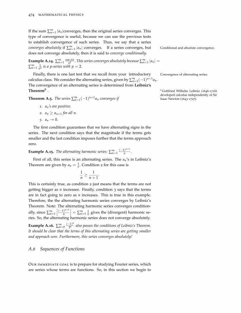
Finally, there is one last test that we recall from your introductory Convergence of alternating series.

calculus class. We consider the alternating series, given by ∑∞n=1(−1)n+1an.

The convergence of an alternating series is determined from Leibniz’sTheorem8 . 8 Gottfried Wilhelm Leibniz (1646-1716)

developed calculus independently of SirIsaac Newton (1643-1727).Theorem A.5. The series ∑∞

n=1(−1)n+1an converges if

1. an’s are positive.

2. an ≥ an+1 for all n.

3. an → 0.

The first condition guarantees that we have alternating signs in theseries. The next condition says that the magnitude if the terms getssmaller and the last condition imposes further that the terms approachzero.

Example A.15. The alternating harmonic series: ∑∞n=1

(−1)n+1

n .

First of all, this series is an alternating series. The an’s in Leibniz’sTheorem are given by an = 1

n . Condition 2 for this case is

1n≥ 1

n + 1.

This is certainly true, as condition 2 just means that the terms are notgetting bigger as n increases. Finally, condition 3 says that the termsare in fact going to zero as n increases. This is true in this example.Therefore, the the alternating harmonic series converges by Leibniz’sTheorem. Note: The alternating harmonic series converges condition-

ally, since ∑∞n=1

∣∣∣ (−1)n+1

n

∣∣∣ = ∑∞n=1

1n gives the (divergent) harmonic se-

ries. So, the alternating harmonic series does not converge absolutely.


(−1)n

2n also passes the conditions of Leibniz’s Theorem.It should be clear that the terms of this alternating series are getting smallerand approach zero. Furthermore, this series converges absolutely!

A.6 Sequences of Functions

Our immediate goal is to prepare for studying Fourier series, whichare series whose terms are functions. So, in this section we begin to


discuss series of functions and the convergence of such series. Oncemore we will need to resort to the convergence of the sequence ofpartial sums. This means we really need to start with sequences offunctions.

Definition A.5. A sequence of functions is simply a set of functionsfn(x), n = 1, 2, . . . defined on a common domain D. A frequently usedexample will be the sequence of functions {1, x, x2, . . .}, x ∈ [−1, 1].

Evaluating each sequences of functions at a given value of x, weobtain a sequence of real numbers. As before, we can ask if this se-quence converges. Doing this for each point in the domain D, we thenask if the resulting collection of limits defines a function on D. Moreformally, this leads us to the idea of pointwise convergence.

Definition A.6. A sequence of functions fn converges pointwise on D Pointwise convergence.

to a limit g iflim

n→∞fn(x) = g(x)

for each x ∈ D. More formally, we write that

limn→∞

fn = g (pointwise on D)

if given x ∈ D and ε > 0, there exists an integer N such that

| fn(x)− g(x)| < ε, ∀n ≥ N.

Example A.17. Consider the sequence of functions

fn(x) =1

1 + nx, |x| < ∞, n = 1, 2, 3, . . . .

The limits depends on the value of x. We consider two cases, x = 0 andx 6= 0.

1. x = 0. Here limn→∞ fn(0) = limn→∞ 1 = 1.

2. x 6= 0. Here limn→∞ fn(x) = limn→∞1

1+nx = 0.

Therefore, we can say that fn → g pointwise for |x| < ∞, where

g(x) =

{0, x 6= 0,1, x = 0.

(A.7)

We also note that in Definition A.6 N generally depends on both xand ε.

Example A.18. We consider the functions fn(x) = xn, x ∈ [0, 1], n =

1, 2, . . . . We recall that the definition for pointwise convergence suggests thatfor each x we seek an N such that | fn(x)− g(x)| < ε, ∀n ≥ N. This is notat first easy to see. So, we will provide some simple examples showing how Ncan depend on both x and ε.


1. x = 0. Here we have fn(0) = 0 for all n. So, given ε > 0 we seekan N such that | fn(0)− 0| < ε, ∀n ≥ N. Inserting fn(0) = 0, wehave 0 < ε. Since this is true for all n, we can pick N = 1.

−1 −0.5 0 0.5 1−1

−0.5

0

0.5

1

x

f n(x)

Plot of fn(x) = xn vs x

Figure A.9: Plot of fn(x) = xn showinghow N depends on x = 0, 0.1, 0.5, 0.9 (thevertical lines) and ε = 0.1 (the horizontalline). Look at the intersection of a givenvertical line with the horizontal line anddetermine N from the number of curvesnot under the intersection point.

2. x = 12 . In this case we have fn(

12 ) = 1

2n , for n = 1, 2, . . . . As ngets large, fn → 0. So, given ε > 0, we seek N such that | 1

2n − 0| <ε, ∀n ≥ N. This means that 1

2n < ε. Solving the inequality forn, we have n > − ln ε

ln 2 We choose N ≥ − ln εln 2 . Thus, our choice of

N depends on ε. For, ε = 0.1, this gives

N ≥ − ln 0.1ln 2

=ln 10ln 2

≈ 3.32.

So, we pick N = 4 and we have n > N = 4.

3. x = 110 . This can be examined like the last example. We have

fn(1

10 ) = 110n , for n = 1, 2, . . . . This leads to N ≥ − ln ε

ln 10 Forε = 0.1, this gives N ≥ 1, or n > 1.

4. x = 910 . This can be examined like the last two examples. We have

fn(9

10 ) =( 9

10)n

, for n = 1, 2, . . . . So given an ε > 0, we seek anN such that

( 910)n

< ε for all n > N. Therefore,

n > N ≥ ln ε

ln( 9

10) .

For ε = 0.1, we have N ≥ 21.85, or n > N = 22.

So, for these cases, we have shown that N can depend on both x and ε.These cases are shown in Figure A.9.

There are other questions that can be asked about sequences of func-tions. Let the sequence of functions fn be continuous on D. If the se-quence of functions converges pointwise to g on D then we can askthe following.

1. Is g continuous on D?

2. If each fn is integrable on [a, b], then does

limn→∞

∫ b

afn(x) dx =

∫ b

ag(x) dx?

3. If each fn is differentiable at c, then does

limn→∞

f ′n(c) = g′(c)?

It turns out that pointwise convergence is not enough to providean affirmative answer to any of these questions. Though we will notprove it here, what we will need is uniform convergence.

−1 0 1−2

−1.5

−1

−0.5

0

0.5

1

1.5

2

2.5Uniform Convergence

x

f n(x)

g(x)

g(x)+ε

g(x)−ε

Figure A.10: For uniform convergence,as n gets large, fn(x) lies in the bandg(x)− ε, g(x)− ε.


Definition A.7. Consider a sequence of functions { fn(x)}∞n=1 on D.

Let g(x) be defined for x ∈ D. Then the sequence converges uniformlyon D, or

limn→∞

fn = g uniformly on D,

if given ε > 0, there exists an N such that

| fn(x)− g(x)| < ε, ∀n ≥ N and ∀x ∈ D.

This definition almost looks like the definition for pointwise con-vergence. However, the seemingly subtle difference lies in the fact thatN does not depend upon x. The sought N works for all x in the do-main. As seen in Figure A.10 as n gets large, fn(x) lies in the band(g(x)− ε, g(x) + ε).

Example A.19. fn(x) = xn, for x ∈ [0, 1].

−1 −0.5 0 0.5 1−1

−0.5

0

0.5

1

g(x) + ε

g(x)− ε

x

f n(x)

Plot of fn(x) = xn vs x

Figure A.11: Plot of fn(x) = xn on [-1,1]for n = 1 . . . 10 and g(x)± ε for ε = 0.2.

Note that in this case as n gets large, fn(x) does not lie in the band (g(x)−ε, g(x) + ε). This is displayed in Figure A.11.

Example A.20. fn(x) = cos(nx)/n2 on [−1, 1].For this example we plot the first several members of the sequence in Figure

A.12. We can see that eventually (n ≥ N) members of this sequence do lieinside a band of width ε about the limit g(x) ≡ 0 for all values of x. Thus,this sequence of functions will converge uniformly to the limit.

−3 −2 −1 0 1 2 3

−0.4

−0.2

0

0.2

0.4

g(x) + ε

g(x)− ε

x

f n(x)

Plot of fn(x) = cos(nx)/n2 vs x

Figure A.12: Plot of fn(x) = cos(nx)/n2

on [−π, π] for n = 1 . . . 10 and g(x)± εfor ε = 0.2.

Finally, we should note that if a sequence of functions is uniformlyconvergent then it converges pointwise. However, the examples shouldbear out that the converse is not true.

A.7 Infinite Series of Functions

We now turn our attention to infinite series of functions, which willform the basis of our study of Fourier series. An infinite series of func-tions is given by ∑∞

n=1 fn(x), x ∈ D. Using powers of x again, anexample would be ∑∞

n=1 xn, x ∈ [−1, 1]. In order to investigate theconvergence of this series; i.e., we would substitute values for x anddetermine if the resulting series of numbers converges. This meansthat we would need to consider the Nth partial sums

sN(x) =N

∑n=1

fn(x).

Does this sequence of functions converge? We begin to answer thisquestion by defining pointwise and uniform convergence.

Definition A.8. ∑ f j(x) converges pointwise to f (x) on D if given x ∈ D,

Pointwise convergence.


and ε > 0, there exists and N such that

| f (x)− sn(x)| < ε

for all n > N.

Definition A.9. ∑ f j(x) converges uniformly to f (x) on D given ε > 0, Uniform convergence.

there exists and N such that

| f (x)− sn(x)| < ε

for all n > N and all x ∈ D.

Again, we state without proof the following:

Uniform convergence give nice proper-ties under some additional conditions,such as being able to integrate, or dif-ferentiate, term by term.

1. Uniform convergence implies pointwise convergence.

2. If fn is continuous on D, and ∑∞n fn converges uniformly to

f on D, then f is continuous on D.

3. If fn is continuous on [a, b] ⊂ D, ∑∞n fn converges uniformly

on D, and∫ b

a fn(x) dx exists, then

∞

∑n

∫ b

afn(x) dx =

∫ b

a

∞

∑n

fn(x) dx =∫ b

ag(x) dx.

4. If f ′n is continuous on [a, b] ⊂ D, ∑∞n fn converges point-

wise to g on D, and ∑∞n f ′n converges uniformly on D, then

∑∞n f ′n(x) = d

dx (∑∞n fn(x)) = g′(x) for x ∈ (a, b).

Since uniform convergence of series gives so much, like term byterm integration and differentiation, we would like to be able to rec-ognize when we have a uniformly convergent series. One test for suchconvergence is the Weierstraß M-Test9.

9 Karl Theodor Wilhelm Weierstraß(1815-1897) was a German mathemati-cian who may be thought of as thefather of analysis.

Theorem A.6. Weierstraß M-Test Let { fn}∞n=1 be a sequence of functions

on D. If | fn(x)| ≤ Mn, for x ∈ D and ∑∞n=1 Mn converges, then ∑∞

n=1 fn

converges uniformly of D.

Proof. First, we note that for x ∈ D,

∞

∑n=1| fn(x)| ≤

∞

∑n=1

Mn.

Thus, since by the assumption that ∑∞n=1 Mn converges, we have that

∑∞n=1 fn converges absolutely on D. Therefore, ∑∞

n=1 fn converges point-wise on D. So, let ∑∞

n=1 fn = g.We now want to prove that this convergence is in fact uniform.

Given ε > 0, we need to find an N such that

|g(x)−n

∑j=1

f j(x)| < ε


if n ≥ N for all x ∈ D.So, for any x ∈ D,

|g(x)−n

∑j=1

f j(x)| = |∞

∑j=1

f j(x)−n

∑j=1

f j(x)|

= |∞

∑j=n+1

f j(x)|

≤∞

∑j=n+1

| f j(x)|, by the triangle inequality

≤∞

∑j=n+1

Mj. (A.8)

Now, the sum over the Mj’s is convergent, so we can choose N suchthat

∞

∑j=n+1

Mj < ε, n ≥ N.

Then, we have from above that

|g(x)−n

∑j=1

f j(x)| ≤∞

∑j=n+1

Mj < ε

for all n ≥ N and x ∈ D. Thus, ∑ f j → g uniformly on D.

We now given an example of how to use the Weierstraß M-Test.

Example A.21. We consider the series ∑∞n=1

cos nxn2 defined on [−π, π]. Each

term is bounded by∣∣∣ cos nx

n2

∣∣∣ = 1n2 ≡ Mn. We know that ∑∞

n=1 Mn =

∑∞n=1

1n2 < ∞. Thus, we can conclude that the original series converges uni-

formly, as it satisfies the conditions of the Weierstraß M-Test.

A.8 Power Series

A typical example of a series of functions that the student hasencountered in previous courses is the power series. Examples of suchseries were provided by Taylor and Maclaurin series.10 10 Actually, what are now known as Tay-

lor and Maclaurin series were knownlong before they were named. JamesGregory (1638-1675) has been recog-nized for discovering Taylor series,which were later named after Brook Tay-lor (1685-1731) . Similarly, Colin Maclau-rin (1698-1746) did not actually discoverMaclaurin series, but because of his par-ticular use of them.

Definition A.10. A power series expansion about x = a with coefficientsequence cn is given by ∑∞

n=0 cn(x− a)n.

For now we will consider all constants to be real numbers with x insome subset of the set of real numbers.

An example of such a power series is the following expansion aboutx = 0 :

∞

∑n=0

xn = 1 + x + x2 + . . . . (A.9)


We would like to make sense of such expansions. For what valuesof x will this infinite series converge? Until now we did not pay muchattention to which infinite series might converge. However, this par-ticular series is already familiar to us. It is a geometric series. Notethat each term is gotten from the previous one through multiplicationby r = x. The first term is a = 1. So, from Equation (1.74), we have thesum of the series is given by

∞

∑n=0

xn =1

1− x, |x| < 1.

In this case we see that the sum, when it exists, is a simple function.In fact, when x is small, we can use this infinite series to provideapproximations to the function (1 − x)−1. If x is small enough, wecan write

(1− x)−1 ≈ 1 + x.

In Figure A.13 we see that for small values of x these functions doagree.

−0.1 0 0.10.9

0.95

1

1.05

1.1

1.15Comparison of 1/(1−x) and 1+x

x

Figure A.13: Comparison of 11−x (solid)

to 1 + x (dashed) for x ∈ [−0.1, 0.1].

Of course, if we want better agreement, we select more terms. InFigure A.14 we see what happens when we do so. The agreement ismuch better. But extending the interval, we see in Figure A.15 showsthat keeping only quadratic terms may not be good enough. Keepingthe cubic terms gives better agreement over the interval.

−0.1 0 0.10.9

0.95

1

1.05

1.1

1.15Comparison of 1/(1−x) and 1+x+x2

x


to 1+ x + x2 (dashed) for x ∈ [−0.1, 0.1].

Finally, in Figure A.16 we show the sum of the first 21 terms overthe entire interval [−1, 1]. Note that there are problems with approxi-mations near the endpoints of the interval, x = ±1.

Such polynomial approximations are called Taylor polynomials. Thus,T3(x) = 1 + x + x2 + x3 is the third order Taylor polynomial approxi-mation of f (x) = 1

1−x .With this example we have seen how useful a series representation

might be for a given function. However, the series representation was asimple geometric series, which we already knew how to sum. Is therea way to begin with a function and then find its series representation?Once we have such a representation, will the series converge to thefunction with which we started? For what values of x will it converge?These questions can be answered by recalling the definitions of Taylorand Maclaurin series.

−0.5 −0.4 −0.3 −0.2 −0.1 0 0.1 0.2 0.3 0.4 0.50.6

0.8

1

1.2

1.4

1.6

1.8

2Comparison of 1/(1−x) 1+x+x2 and 1+x+x2+x3

x


to 1+ x+ x2 (dashed) and 1+ x+ x2 + x3

(dash-dot) for x ∈ [−0.5, 0.5].

Definition A.11. A Taylor series expansion of f (x) about x = a is the

Taylor series expansion.

series

f (x) ∼∞

∑n=0

cn(x− a)n, (A.10)

where

cn =f (n)(a)

n!. (A.11)


Note that we use ∼ to indicate that we have yet to determine whenthe series may converge to the given function. A special class of seriesare those Taylor series for which the expansion is about x = 0.

Definition A.12. A Maclaurin series expansion of f (x) is a Taylor seriesexpansion of f (x) about x = 0, or Maclaurin series expansion.

f (x) ∼∞

∑n=0

cnxn, (A.12)

where

cn =f (n)(0)

n!. (A.13)

−1−0.9−0.8−0.7−0.6−0.5−0.4−0.3−0.2−0.1 0 0.10.20.30.40.50.60.70.80.9 10

0.5

1

1.5

2

2.5

3

3.5

4

4.5

5

Comparison of 1/(1−x) to Σn=020 xn

x


to ∑∞n=0 xn for x ∈ [−1, 1].

Example A.22. Expand f (x) = ex about x = 0.We begin by creating a table. In order to compute the expansion coeffi-

cients, cn, we will need to perform repeated differentiations of f (x). So, weprovide a table for these derivatives. Then we only need to evaluate the secondcolumn at x = 0 and divide by n!.

n f (n)(x) cn

0 ex e0

0! = 1

1 ex e0

1! = 1

2 ex e0

2! =12!

3 ex e0

3! =13!

Next, one looks at the last column and tries to determine some pattern soas to write down the general term of the series. If there is only a need to get apolynomial approximation, then the first few terms may be sufficient.

In this case, we have that the pattern is obvious: cn = 1n! . So,

ex ∼∞

∑n=0

xn

n!.

Example A.23. Expand f (x) = ex about x = 1.Here we seek an expansion of the form ex ∼ ∑∞

n=0 cn(x − 1)n. We couldcreate a table like the last example. In fact, the last column would have valuesof the form e

n! . (You should confirm this.) However, we could make use ofthe Maclaurin series expansion for ex and get the result quicker. Note thatex = ex−1+1 = eex−1. Now, apply the known expansion for ex :

ex ∼ e(

1 + (x− 1) +(x− 1)2

2+

(x− 1)3

3!+ . . .

)=

∞

∑n=0

e(x− 1)n

n!.


Example A.24. Expand f (x) = 11−x about x = 0.

This is the example with which we started our discussion. We set up atable again. We see from the last column that we get back our geometric series(A.9).

n f (n)(x) cn

0 11−x

10! = 1

1 1(1−x)2

11! = 1

2 2(1)(1−x)3

2!2! = 1

3 3(2)(1)(1−x)4

3!3! = 1

So, we have found

11− x

∼∞

∑n=0

xn.

We can replace ∼ by equality if we can determine the range of x-values for which the resulting infinite series converges. We will inves-tigate such convergence shortly.

Series expansions for many elementary functions arise in a varietyof applications. Some common expansions are provided below.


Series Expansions You Should Know

ex = 1 + x +x2

2+

x3

3!+

x4

4!+ . . . =

∞

∑n=0

xn

n!(A.14)

cos x = 1− x2

2+

x4

4!− . . . =

∞

∑n=0

(−1)n x2n

(2n)!(A.15)

sin x = x− x3

3!+

x5

5!− . . . =

∞

∑n=0

(−1)n x2n+1

(2n + 1)!(A.16)

cosh x = 1 +x2

2+

x4

4!+ . . . =

∞

∑n=0

x2n

(2n)!(A.17)

sinh x = x +x3

3!+

x5

5!+ . . . =

∞

∑n=0

x2n+1

(2n + 1)!(A.18)

11− x

= 1 + x + x2 + x3 + . . . =∞

∑n=0

xn (A.19)

11 + x

= 1− x + x2 − x3 + . . . =∞

∑n=0

(−x)n (A.20)

tan−1 x = x− x3

3+

x5

5− x7

7+ . . . =

∞

∑n=0

(−1)n x2n+1

2n + 1(A.21)

ln(1 + x) = x− x2

2+

x3

3− . . . =

∞

∑n=1

(−1)n+1 xn

n(A.22)

What is still left to be determined is for what values do such powerseries converge. The first five of the above expansions converge for allreals, but the others only converge for |x| < 1.

We consider the convergence of ∑∞n=0 cn(x− a)n. For x = a the series

obviously converges. Will it converge for other points? One can prove

Theorem A.7. If ∑∞n=0 cn(b− a)n converges for b 6= a, then

∑∞n=0 cn(x− a)n converges absolutely for all x satisfying |x− a| < |b− a|.

This leads to three possibilities

1. ∑∞n=0 cn(x− a)n may only converge at x = a.

2. ∑∞n=0 cn(x− a)n may converge for all real numbers.

3. ∑∞n=0 cn(x − a)n converges for |x − a| < R and diverges for|x− a| > R.

The number R is called the radius of convergence of the power series Interval and radius of convergence.

and (a− R, a + R) is called the interval of convergence. Convergence atthe endpoints of this interval has to be tested for each power series.

In order to determine the interval of convergence, one needs onlynote that when a power series converges, it does so absolutely. So, weneed only test the convergence of ∑∞

n=0 |cn(x − a)n| = ∑∞n=0 |cn||x −


a|n. This is easily done using either the ratio test or the nth root test.We first identify the nonnegative terms an = |cn||x − a|n, using thenotation from Section A.4. Then we apply one of our convergencetests.

For example, the nth Root Test gives the convergence condition

ρ = limn→∞

n√

an = limn→∞

n√|cn||x− a| < 1.

Thus,

|x− a| <(

limn→∞

n√|cn|)−1

≡ R.

This, R is the radius of convergence.Similarly, we can apply the Ratio Test.

ρ = limn→∞

an+1

an= lim

n→∞

|cn+1||cn|

|x− a| < 1.

Again, we rewrite this result to determine the radius of convergence:

|x− a| <(

limn→∞

|cn+1||cn|

)−1

≡ R.

Example A.25. ex = ∑∞n=0

xn

n! .Since there is a factorial, we will use the Ratio Test with a = 0..

ρ = limn→∞

|n!||(n + 1)!| |x| = lim

n→∞

1n + 1

|x| = 0.

Since ρ = 0, it is independent of |x| and thus the series converges for all x.We also can say that the radius of convergence is infinite.

Example A.26. 11−x = ∑∞

n=0 xn.In this example we will use the nth Root Test with a = 0.

ρ = limn→∞

n√1|x| = |x| < 1.

Thus, we find that we have absolute convergence for |x| < 1. Setting x = 1 orx = −1, we find that the resulting series do not converge. So, the endpointsare not included in the complete interval of convergence.

In this example we could have also used the Ratio Test. Thus,

ρ = limn→∞

11|x| = |x| < 1.

We have obtained the same result as when we used the nth Root Test.


3n(x−2)n

n .In this example, we have an expansion about x = 2. Using the nth Root

Test we find that

ρ = limn→∞

n

√3n

n|x− 2| = 3|x− 2| < 1.


Solving for |x− 2| in this inequality, we find |x− 2| < 13 . Thus, the radius

of convergence is R = 13 and the interval of convergence is

(2− 1

3 , 2 + 13

)=( 5

3 , 73)

.As for the endpoints, we need to first test at x = 7

3 . The resulting series

is ∑∞n=1

3n( 13 )

n

n = ∑∞n=1

1n . This is the harmonic series, and thus it does not

converge. Inserting x = 53 we get the alternating harmonic series, which does

converge. So, we have convergence on [ 53 , 7

3 ). However, it is only conditionallyconvergent at the left endpoint, x = 5

3 .

Example A.28. Find an expansion of f (x) = 1x+2 about x = 1.

Instead of explicitly computing the Taylor series expansion for this func-tion, we can make use of an already known function. We first write f (x) as afunction of x− 1, since we are expanding about x = 1. This is easily done bynoting that 1

x+2 = 1(x−1)+3 . Factoring out a 3, we can rewrite this as a sum

of a geometric series. Namely, we use the expansion for

g(z) =1

1 + z= 1− z + z2 − z3 + . . . . (A.23)

and then we rewrite f (x) as

f (x) =1

x + 2

=1

(x− 1) + 3

=1

3[1 + 13 (x− 1)]

=13

11 + 1

3 (x− 1). (A.24)

Note that f (x) = 13 g( 1

3 (x− 1)) for g(z) = 11+z So, the expansion becomes

f (x) =13

[1− 1

3(x− 1) +

(13(x− 1)

)2−(

13(x− 1)

)3+ . . .

].

This can further be simplified as

f (x) =13− 1

9(x− 1) +

127

(x− 1)2 − . . . .

Convergence is easily established. The expansion for g(z) converges for|z| < 1. So, the expansion for f (x) converges for | − 1

3 (x − 1)| < 1. Thisimplies that |x − 1| < 3. Putting this inequality in interval notation, wehave that the power series converges absolutely for x ∈ (−2, 4). Inserting theendpoints, one can show that the series diverges for both x = −2 and x = 4.You should verify this!


Euler’s Formula, eiθ = cos θ + i sin θ, isan important formula and will be usedthroughout the text.

As a final application, we can derive Euler’s Formula ,

eiθ = cos θ + i sin θ,

where i =√−1. We naively use the expansion for ex with x = iθ. This

leads us to

eiθ = 1 + iθ +(iθ)2

2!+

(iθ)3

3!+

(iθ)4

4!+ . . . .

Next we note that each term has a power of i. The sequence ofpowers of i is given as {1, i,−1,−i, 1, i,−1,−i, 1, i,−1,−i, . . .}. See thepattern? We conclude that

in = ir, where r = remainder after dividing n by 4.

This gives

eiθ =

(1− θ2

2!+

θ4

4!− . . .

)+ i(

θ − θ3

3!+

θ5

5!− . . .

).

We recognize the expansions in the parentheses as those for the cosineand sine functions. Thus, we end with Euler’s Formula.

We further derive relations from this result, which will be importantfor our next studies. From Euler’s formula we have that for integer n:

einθ = cos(nθ) + i sin(nθ).

We also haveeinθ =

(eiθ)n

= (cos θ + i sin θ)n .

Equating these two expressions, we are led to de Moivre’s Formula,named after Abraham de Moivre (1667-1754),

(cos θ + i sin θ)n = cos(nθ) + i sin(nθ). (A.25)

Here we see elegant proofs of wellknown trigonometric identities. We willlater make extensive use of these identi-ties. Namely, you should know:

cos 2θ = cos2 θ − sin2 θ, (A.26)

sin 2θ = 2 sin θ cos θ, (A.27)

cos2 θ =12(1 + cos 2θ), (A.28)

sin2 θ =12(1− cos 2θ). (A.29)

This formula is useful for deriving identities relating powers of sinesor cosines to simple functions. For example, if we take n = 2 in Equa-tion (A.25), we find

cos 2θ + i sin 2θ = (cos θ + i sin θ)2 = cos2 θ − sin2 θ + 2i sin θ cos θ.

Looking at the real and imaginary parts of this result leads to the wellknown double angle identities

cos 2θ = cos2 θ − sin2 θ, sin 2θ = 2 sin θ cos θ.

Replacing cos2 θ = 1− sin2 θ or sin2 θ = 1− cos2 θ leads to the halfangle formulae:

cos2 θ =12(1 + cos 2θ), sin2 θ =

12(1− cos 2θ).


Trigonometric functions can be writtenin terms of complex exponentials:

cos θ =eiθ + e−iθ

2,

sin θ =eiθ − e−iθ

2i.

We can also use Euler’s Formula to write sines and cosines in termsof complex exponentials. We first note that due to the fact that thecosine is an even function and the sine is an odd function, we have

e−iθ = cos θ − i sin θ.

Combining this with Euler’s Formula, we have that

cos θ =eiθ + e−iθ

2, sin θ =

eiθ − e−iθ

2i.

Hyperbolic functions and trigonometricfunctions are intimately related.

cos(ix) = cosh x,

sin(ix) = −i sinh x.

We finally note that there is a simple relationship between hyper-bolic functions and trigonometric functions. Recall that

cosh x =ex + e−x

2.

If we let x = iθ, then we have that cosh(iθ) = cos θ and cos(ix) =

cosh x. Similarly, we can show that sinh(iθ) = i sin θ and sin(ix) =

−i sinh x. The binomial expansion is a special se-ries expansion used to approximate ex-pressions of the form (a + b)p for b� a,or (1 + x)p for |x| � 1.One series expansion which occurs often in examples and appli-

cations is the binomial expansion. This is simply the expansion ofthe expression (a + b)p in powers of a and b. We will investigate thisexpansion first for nonnegative integer powers p and then derive theexpansion for other values of p. While the binomial expansion canbe obtained using Taylor series, we will provide a more interestingderivation here to show that

(a + b)p =∞

∑ Crpan−rbr, (A.30)

where the Crp are called the binomial coefficients.

One series expansion which occurs often in examples and applica-tions is the binomial expansion. This is simply the expansion of theexpression (a+ b)p. We will investigate this expansion first for nonneg-ative integer powers p and then derive the expansion for other valuesof p.

Lets list some of the common expansions for nonnegative integerpowers.

(a + b)0 = 1

(a + b)1 = a + b

(a + b)2 = a2 + 2ab + b2

(a + b)3 = a3 + 3a2b + 3ab2 + b3

(a + b)4 = a4 + 4a3b + 6a2b2 + 4ab3 + b4

· · · (A.31)


We now look at the patterns of the terms in the expansions. First, wenote that each term consists of a product of a power of a and a powerof b. The powers of a are decreasing from n to 0 in the expansion of(a + b)n. Similarly, the powers of b increase from 0 to n. The sums ofthe exponents in each term is n. So, we can write the (k + 1)st termin the expansion as an−kbk. For example, in the expansion of (a + b)51

the 6th term is a51−5b5 = a46b5. However, we do not yet know thenumerical coefficient in the expansion.

Let’s list the coefficients for the above expansions.

n = 0 : 1n = 1 : 1 1n = 2 : 1 2 1n = 3 : 1 3 3 1n = 4 : 1 4 6 4 1

(A.32)

This pattern is the famous Pascal’s triangle.11 There are many inter-

11 Pascal’s triangle is named after BlaisePascal (1623-1662). While such configu-rations of number were known earlier inhistory, Pascal published them and ap-plied them to probability theory.

Pascal’s triangle has many unusualproperties and a variety of uses:

• Horizontal rows add to powers of 2.

• The horizontal rows are powers of 11

(1, 11, 121, 1331, etc.).

• Adding any two successive numbersin the diagonal 1-3-6-10-15-21-28...results in a perfect square.

• When the first number to the right ofthe 1 in any row is a prime number,all numbers in that row are divisibleby that prime number.

• Sums along certain diagonals leadsto the Fibonacci sequence.

esting features of this triangle. But we will first ask how each row canbe generated.

We see that each row begins and ends with a one. The secondterm and next to last term have a coefficient of n. Next we note thatconsecutive pairs in each row can be added to obtain entries in the nextrow. For example, we have for rows n = 2 and n = 3 that 1 + 2 = 3and 2 + 1 = 3 :

n = 2 : 1 2 1↘ ↙ ↘ ↙

n = 3 : 1 3 3 1(A.33)

With this in mind, we can generate the next several rows of ourtriangle.

n = 3 : 1 3 3 1n = 4 : 1 4 6 4 1n = 5 : 1 5 10 10 5 1n = 6 : 1 6 15 20 15 6 1

(A.34)

So, we use the numbers in row n = 4 to generate entries in row n = 5 :1 + 4 = 5, 4 + 6 = 10. We then use row n = 5 to get row n = 6, etc.

Of course, it would take a while to compute each row up to thedesired n. Fortunately, there is a simple expression for computing aspecific coefficient. Consider the kth term in the expansion of (a + b)n.Let r = k − 1. Then this term is of the form Cn

r an−rbr. We have seenthe the coefficients satisfy

Cnr = Cn−1

r + Cn−1r−1 .


Actually, the binomial coefficients have been found to take a simpleform,

Cnr =

n!(n− r)!r!

≡(

nr

).

This is nothing other than the combinatoric symbol for determininghow to choose n things r at a time. In our case, this makes sense. Wehave to count the number of ways that we can arrange r products of bwith n− r products of a. There are n slots to place the b’s. For example,the r = 2 case for n = 4 involves the six products: aabb, abab, abba,baab, baba, and bbaa. Thus, it is natural to use this notation.

So, we have found that

(a + b)n =n

∑r=0

(nr

)an−rbr. (A.35)

Now consider the geometric series 1 + x + x2 + . . . . We have seenthat such a series converges for |x| < 1, giving

1 + x + x2 + . . . =1

1− x.

But, 11−x = (1− x)−1.

This is again a binomial to a power, but the power is not an integer.It turns out that the coefficients of such a binomial expansion can bewritten similar to the form in Equation (A.35).

This example suggests that our sum may no longer be finite. So, forp a real number, we write

(1 + x)p =∞

∑r=0

(pr

)xr. (A.36)

However, we quickly run into problems with this form. Considerthe coefficient for r = 1 in an expansion of (1 + x)−1. This is given by(

−11

)=

(−1)!(−1− 1)!1!

=(−1)!(−2)!1!

.

But what is (−1)!? By definition, it is

(−1)! = (−1)(−2)(−3) · · · .

This product does not seem to exist! But with a little care, we note that

(−1)!(−2)!

=(−1)(−2)!

(−2)!= −1.

So, we need to be careful not to interpret the combinatorial coefficientliterally. There are better ways to write the general binomial expansion.


We can write the general coefficient as(pr

)=

p!(p− r)!r!

=p(p− 1) · · · (p− r + 1)(p− r)!

(p− r)!r!

=p(p− 1) · · · (p− r + 1)

r!. (A.37)

With this in mind we now state the theorem:

General Binomial Expansion

The general binomial expansion for (1 + x)p is a simple gener-alization of Equation (A.35). For p real, we have the followingbinomial series:

(1 + x)p =∞

∑r=0

p(p− 1) · · · (p− r + 1)r!

xr, |x| < 1. (A.38)

Often we need the first few terms for the case that x � 1 :

(1 + x)p = 1 + px +p(p− 1)

2x2 + O(x3). (A.39)

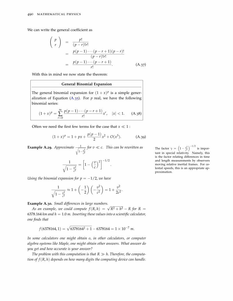
Example A.29. Approximate 1√1− v2

c2

for v� c. This can be rewritten as The factor γ =(

1− v2

c2

)−1/2is impor-

tant in special relativity. Namely, thisis the factor relating differences in timeand length measurements by observersmoving relative inertial frames. For ce-lestial speeds, this is an appropriate ap-proximation.

1√1− v2

c2

=

[1−

(vc

)2]−1/2

.

Using the binomial expansion for p = −1/2, we have

1√1− v2

c2

≈ 1 +(−1

2

)(−v2

c2

)= 1 +

v2

2c2 .

Example A.30. Small differences in large numbers.As an example, we could compute f (R, h) =

√R2 + h2 − R for R =

6378.164 km and h = 1.0 m. Inserting these values into a scientific calculator,one finds that

f (6378164, 1) =√

63781642 + 1− 6378164 = 1× 10−7 m.

In some calculators one might obtain 0, in other calculators, or computeralgebra systems like Maple, one might obtain other answers. What answer doyou get and how accurate is your answer?

The problem with this computation is that R� h. Therefore, the computa-tion of f (R, h) depends on how many digits the computing device can handle.


The best way to get an answer is to use the binomial approximation. Writingx = h

R , we have

f (R, h) =√

R2 + h2 − R

= R√

1 + x2 − R

' R[

1 +12

x2]− R

=12

Rx2

=12

hR2 = 7.83926× 10−8 m. (A.40)

Of course, you should verify how many digits should be kept in reporting theresult.

In the next examples, we show how computations taking a moregeneral form can be handled. Such general computations appear inproofs involving general expansions without specific numerical valuesgiven.

Example A.31. Obtain an approximation to (a + b)p when a is much largerthan b, denoted by a� b.

If we neglect b then (a + b)p ' ap. How good of an approximation isthis? This is where it would be nice to know the order of the next term in theexpansion. Namely, what is the power of b/a of the first neglected term inthis expansion?

In order to do this we first divide out a as

(a + b)p = ap(

1 +ba

)p.

Now we have a small parameter, ba . According to what we have seen earlier,

we can use the binomial expansion to write(1 +

ba

)n=

∞

∑r=0

(pr

)(ba

)r. (A.41)

Thus, we have a sum of terms involving powers of ba . Since a � b, most of

these terms can be neglected. So, we can write(1 +

ba

)p= 1 + p

ba+ O

((ba

)2)

.

Here we used O(), big-Oh notation, to indicate the size of the first neglectedterm. (This notation is formally defined in another section.)

Summarizing, this then gives

(a + b)p = ap(

1 +ba

)p


= ap

(1 + p

ba+ O

((ba

)2))

= ap + pap ba+ apO

((ba

)2)

. (A.42)

Therefore, we can approximate (a + b)p ' ap + pbap−1, with an error onthe order of b2ap−2. Note that the order of the error does not include theconstant factor from the expansion. We could also use the approximation that(a + b)p ' ap, but it is not typically good enough in applications because theerror in this case is of the order bap−1.

Example A.32. Approximate f (x) = (a + x)p − ap for x� a.In an earlier example we computed f (R, h) =

√R2 + h2 − R for R =

6378.164 km and h = 1.0 m. We can make use of the binomial expansion todetermine the behavior of similar functions in the form f (x) = (a+ x)p− ap.Inserting the binomial expression into f (x), we have as x

a → 0 that

f (x) = (a + x)p − ap

= ap[(

1 +xa

)p− 1]

= ap[

pxa

+ O(( x

a

)2)]

= O( x

a

)as

xa→ 0. (A.43)

This result might not be the approximation that we desire. So, we couldback up one step in the derivation to write a better approximation as

(a + x)p − ap = ap−1 px + O(( x

a

)2)

asxa→ 0.

We could use this approximation to answer the original question by lettinga = R2, x = 1 and p = 1

2 . Then, our approximation would be of order

O(( x

a

)2)= O

((1

63781642

)2)∼ 2.4× 10−14.

Thus, we have √63781642 + 1− 6378164 ≈ ap−1 px

whereap−1 px = (63781642)−1/2(0.5)1 = 7.83926× 10−8.

This is the same result we had obtained before.

A.9 The Order of Sequences and Functions

Often we are interested in comparing the rates of convergenceof sequences or asymptotic behavior of functions. This is useful in


approximation theory as we had seen in the last section. We beginwith the comparison of sequences and introduce big-Oh notation. Wewill then extend this to functions of continuous variables.

Definition A.13. Let {an} and {bn} be two sequences. Then if thereare numbers N and K (independent of N) such that∣∣∣∣ an

bn

∣∣∣∣ < K whenever n > N,

then we say that an is of the order of bn. We write this as

an = O(bn) as n→ ∞

and say an is “big O” of bn.

Example A.33. Consider the sequences given by an = 2n+13n2+2 and bn = 1

n .In this case we consider the ratio,∣∣∣∣ an

bn

∣∣∣∣ =∣∣∣∣∣

2n+13n2+2

1n

∣∣∣∣∣ =∣∣∣∣2n2 + n

3n2 + 2

∣∣∣∣ .

We want to find a bound on the last expression as n gets large. We dividethe numerator and denominator by n2 and find that∣∣∣∣ an

bn

∣∣∣∣ = ∣∣∣∣ 2 + 1/n3 + 2/n2

∣∣∣∣ = 23

∣∣∣∣ 1 + 1/2n1 + 2/3n2

∣∣∣∣ .

The last expresssion is largest for n = 1. This gives∣∣∣∣ an

bn

∣∣∣∣ = 23

∣∣∣∣ 1 + 1/2n1 + 2/3n2

∣∣∣∣ ≤ 23

∣∣∣∣1 + 1/21 + 2/3

∣∣∣∣ = 910

.

Thus, for n > 1, we have that∣∣∣∣ an

bn

∣∣∣∣ ≤ 910

< 1 ≡ K.

We then conclude from Definition A.13 that

an = O(bn) = O(

1n

).

In practice one is often given a sequence like an, but the secondsimpler sequence needs to be found by looking at the large n behaviorof an.

Referring to the last example, we are given an = 2n+13n2+2 . We look

at the large n behavior. The numerator behaves like 2n and the de-nominator behaves like 3n2. Thus, an = 2n+1

3n2+2 ∼2n3n2 = 2

3n for large n.Therefore, we say that an = O( 1

n ) for large n. Note that we are only in-terested in the n-dependence and not the multiplicative constant since1n and 2

3n have the same growth rate.In a similar way, we can compare functions. We modify our defini-

tion of big-Oh for functions of a continuous variable.


Definition A.14. f (x) is of the order of g(x), or f (x) = O(g(x)) asx → x0 if

limx→x0

∣∣∣∣ f (x)g(x)

∣∣∣∣ < K

for some K independent of x0.

Example A.34. Show that

cos x− 1 +x2

2= O(x4) as x → 0.

This should be apparent from the Taylor series expansion for cos x,

cos x = 1− x2

2+ O(x4) as x → 0.

However, we will show that cos x− 1 + x2

2 is of the order of O(x4) using theabove definition.

We need to compute

limx→0

∣∣∣∣∣cos x− 1 + x2

2x4

∣∣∣∣∣ .

The numerator and denominator separately go to zero, so we have an indeter-minate form. This suggests that we need to apply L’Hopital’s Rule. In fact,we apply it several times to find that

limx→0

∣∣∣∣∣cos x− 1 + x2

2x4

∣∣∣∣∣ = limx→0

∣∣∣∣− sin x + x4x3

∣∣∣∣= lim

x→0

∣∣∣∣− cos x + 112x2

∣∣∣∣= lim

x→0

∣∣∣∣ sin x24x

∣∣∣∣ = 124

.

Thus, for any number K > 124 , we have that

limx→0

∣∣∣∣∣cos x− 1 + x2

2x4

∣∣∣∣∣ < K.

We conclude that

cos x− 1 +x2

2= O(x4) as x → 0.

Example A.35. Determine the order of f (x) = (x3 − x)1/3 − x as x →∞. We can use a binomial expansion to write the first term in powers of x.However, since x→ ∞, we want to write f (x) in powers of 1

x , so that we canneglect higher order powers. We can do this by first factoring out the x3 :

(x3 − x)1/3 − x = x(

1− 1x2

)1/3− x


= x(

1− 13x2 + O

(1x4

))− x

= − 13x

+ O(

1x3

). (A.44)

Now we can see from the first term on the right that (x3 − x)1/3 − x =

O(

1x

)as x → ∞.

Problems

1. For those sequences that converge, find the limit limn→∞ an.

a. an = n2+1n3+1 .

b. an = 3n+1n+2 .

c. an =( 3

n)1/n

.

d. an = 2n2+4n3

n3+5√

2+n6 .

e. an = n ln(

1 + 1n

).

f. an = n sin(

1n

).

g. an = (2n+3)!(n+1)! .

2. Find the sum for each of the series:

a. ∑∞n=0

(−1)n34n .

b. ∑∞n=2

25n .

c. ∑∞n=0

(5

2n + 13n

).

d. ∑∞n=1

3n(n+3) .

3. Determine if the following converge, or diverge, using one of theconvergence tests. If the series converges, is it absolute or conditional?

a. ∑∞n=1

n+42n3+1 .

b. ∑∞n=1

sin nn2 .

c. ∑∞n=1

( nn+1)n2

.

d. ∑∞n=1(−1)n n−1

2n2−3 .

e. ∑∞n=1

ln nn .

f. ∑∞n=1

100n

n200 .

g. ∑∞n=1(−1)n n

n+3 .

h. ∑∞n=1(−1)n

√5n

n+1 .

4. Do the following:


a. Compute: limn→∞ n ln(1− 3

n)

.

b. Use L’Hopital’s Rule to evaluate L = limx→∞

(1− 4

x

)x. Hint:

Consider ln L.

c. Determine the convergence of ∑∞n=1

( n3n+2

)n2.

d. Sum the series ∑∞n=1

[tan−1 n− tan−1(n + 1)

]by first writing

the Nth partial sum and then computing limN→∞ sN .

5. Consider the sum ∑∞n=1

1(n+2)(n+1) .

a. Use an appropriate convergence test to show that this seriesconverges.

b. Verify that

∞

∑n=1

1(n + 2)(n + 1)

=∞

∑n=1

(n + 1n + 2

− nn + 1

).

c. Find the nth partial sum of the series ∑∞n=1

(n+1n+2 −

nn+1

)and

use it to determine the sum of the resulting telescoping series.

6. Recall that the alternating harmonic series converges conditionally.

a. From the Taylor series expansion for f (x) = ln(1+ x), insert-ing x = 1 gives the alternating harmonic series. What is thesum of the alternating harmonic series?

Since the alternating harmonic series does not converge absolutely,then a rearrangement of the terms in the series will result in serieswhose sums vary. One such rearrangement in alternating p positiveterms and n negative terms leads to the following sum12: 12 This is discussed by Lawrence H. Rid-

dle in the Kenyon Math. Quarterly, 1(2),6-21.1

2ln

4pn

=

(1 +

13+ · · ·+ 1

2p− 1

)︸︷︷︸

p terms

−(

12+

14+ · · ·+ 1

2n

)︸︷︷︸

n terms

+

(1

2p + 1+ · · ·+ 1

4p− 1

)︸︷︷︸

p terms

−(

12n + 2

+ · · ·+ 14n

)︸︷︷︸

n terms

+ · · · .

Find rearrangements of the alternating harmonic series to give the fol-lowing sums; i.e., determine p and n for the given expression and writedown the above series explicitly; i.e, determine p and n leading to thefollowing sums.

b. 52 ln 2.

c. ln 8.

d. 0.

e. A sum that is close to π.


7. Determine the radius and interval of convergence of the followinginfinite series:

a. ∑∞n=1(−1)n (x−1)n

n .

b. ∑∞n=1

xn

2nn! .

c. ∑∞n=1

1n( x

5)n

d. ∑∞n=1(−1)n xn

√n .

8. Find the Taylor series centered at x = a and its correspondingradius of convergence for the given function. In most cases, you neednot employ the direct method of computation of the Taylor coefficients.

a. f (x) = sinh x, a = 0.

b. f (x) =√

1 + x, a = 0.

c. f (x) = xex, a = 1.

d. f (x) = x−12+x , a = 1.

9. Test for pointwise and uniform convergence on the given set. [TheWeierstraß M-Test might be helpful.]

a. f (x) = ∑∞n=1

ln nxn2 , x ∈ [1, 2].

b. f (x) = ∑∞n=1

13n cos x

2n on R.

10. Consider Gregory’s expansion

tan−1 x = x− x3

3+

x5

5− · · · =

∞

∑k=0

(−1)k

2k + 1x2k+1.

a. Derive Gregory’s expansion by using the definition

tan−1 x =∫ x

0

dt1 + t2 ,

expanding the integrand in a Maclaurin series, and integrat-ing the resulting series term by term.

b. From this result, derive Gregory’s series for π by insertingan appropriate value for x in the series expansion for tan−1 x.

11. Use deMoivre’s Theorem to write sin3 θ in terms of sin θ and sin 3θ.Hint: Focus on the imaginary part of e3iθ .

12. Evaluate the following expressions at the given point. Use yourcalculator and your computer (such as Maple). Then use series ex-pansions to find an approximation to the value of the expression to asmany places as you trust.

a. 1√1+x3 − cos x2 at x = 0.015.

b. ln√

1+x1−x − tan x at x = 0.0015.


c. f (x) = 1√1+2x2 − 1 + x2 at x = 5.00× 10−3.

d. f (R, h) = R−√

R2 + h2 for R = 1.374× 103 km and h = 1.00m.

e. f (x) = 1− 1√1−x

for x = 2.5× 10−13.

13. Determine the order, O(xp), of the following functions. You mayneed to use series expansions in powers of x when x → 0, or seriesexpansions in powers of 1/x when x → ∞.

a.√

x(1− x) as x → 0.

b. x5/4

1−cos x as x → 0.

c. xx2−1 as x → ∞.

d.√

x2 + x− x as x → ∞.

Documents

A Review of Sequences and Inﬁnite Seriespeople.uncw.edu/hermanr/phy311/MathPhysBook/Series.pdfA Review of Sequences and Inﬁnite Series “Once you eliminate the impossible, whatever