Paper PR02

A REVIEW OF PROPENSITY SCORE APPLICATION IN HEALTHCARE OUTCOME AND EPIDEMIOLOGY

Guiping Yang, Premier Inc., Charlotte, NC

Stephen Stemkowski, Premier Inc., Charlotte, NC William Saunders, Premier Inc., Charlotte, NC

ABSTRACT Propensity score approaches in outcomes and epidemiological research are most often used for sample selection by matching, analysis of causal effect by stratification, or risk adjustment by combining propensity score and regression models. Several computing tools are available including SAS, S-PLUS/R, and SPSS to develop and implement propensity score approaches in a variety of applications. This paper reviews the history, statistical definitions, and application of the propensity score in non-randomized observational studies, pre-estimation for randomized designs, and poorly randomized experiments. Several distinct propensity score matching methods, both simple and sophisticated are described in detail to enable users to choose the most appropriate solutions to fit their study objectives. Special cases of propensity score applications discussed include multi-treatment studies, multi-control designs, and missing data processing, where the definitions, estimations and utilization of propensity scores are far different from the general, treatment-control approach. Finally, a discussion of the limitations of propensity score applications in health services and pharmaceutical outcomes research is included. KEYWORDS: Observational study, propensity score, selection bias, matching INTRODUCTION Firstly, let’s look at a typical example of Simpson’s Paradox (Obenchain, 2005):

Hospital Type Severity of Illness

Mild (Mortality Rate %)

Severe (Mortality Rate %)

Total (Mortality Rate %)

World-Class Hospitals 3/327 (1%) 41/678 (6%) 44/1,005 (4.4%)

Local Hospitals 8/258 (3%) 3/33 (9%) 11/291 (3.8%)

Total 11/585 (2%) 44/711 (3%) This is an investigation for comparison of mortality rate between two types of hospitals. In this example, we can see, more severe patients would select world-class hospitals, where more sophisticated diagnostic capabilities and more experienced physicians are available, and yet have higher mortality rates in mild and severe patients when considered together. Thus, treatment selection is not independent of severity of disease. Severity of patient disease is a confounding factor when we compare treatment effects in terms of patient mortality rate. This phenomenon occurs frequently in pharmaceutical and healthcare researches, it is a typical ‘Apples to oranges’ comparison. The distribution balance of the treatment and control groups is always crucial in experimental designs in pharmaceutical or health outcome studies, where randomization is a major tool to avoid biased comparisons. This ‘Gold Standard’ of evaluation has been adopted for a relatively long period to ‘guarantee’ the scientific validity of findings by both statistical professionals and medical experts. In some cases, however, randomization is quite deceptive because of either immeasurable characteristics (e.g. ethic issues) or infeasibility in terms of cost and time. Also, the integrity of the evaluation may be threatened due to failure of subjects in the study to follow protocols, morbidity or mortality, or other reasons for dropping out. Under these circumstances, observational study gains more attention with respect to assessment accuracy if the investigator could adjust for the large confounding biases. Like experiments, in observational studies, a

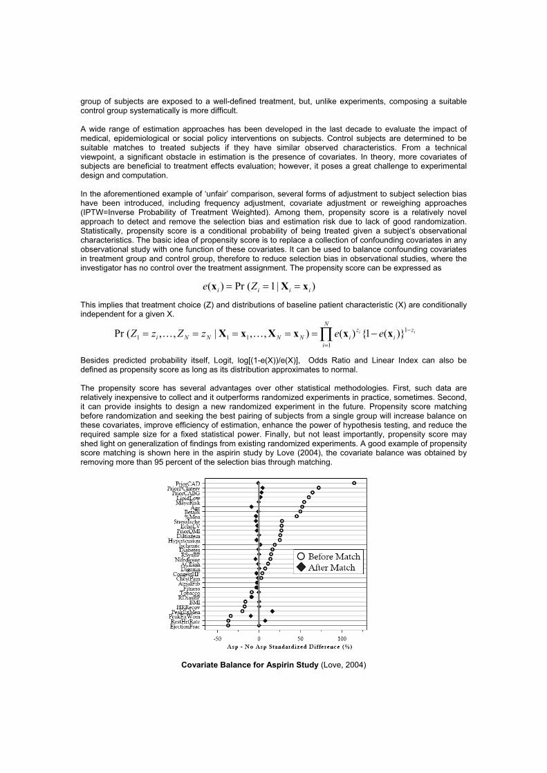
group of subjects are exposed to a well-defined treatment, but, unlike experiments, composing a suitable control group systematically is more difficult. A wide range of estimation approaches has been developed in the last decade to evaluate the impact of medical, epidemiological or social policy interventions on subjects. Control subjects are determined to be suitable matches to treated subjects if they have similar observed characteristics. From a technical viewpoint, a significant obstacle in estimation is the presence of covariates. In theory, more covariates of subjects are beneficial to treatment effects evaluation; however, it poses a great challenge to experimental design and computation. In the aforementioned example of ‘unfair’ comparison, several forms of adjustment to subject selection bias have been introduced, including frequency adjustment, covariate adjustment or reweighing approaches (IPTW=Inverse Probability of Treatment Weighted). Among them, propensity score is a relatively novel approach to detect and remove the selection bias and estimation risk due to lack of good randomization. Statistically, propensity score is a conditional probability of being treated given a subject’s observational characteristics. The basic idea of propensity score is to replace a collection of confounding covariates in any observational study with one function of these covariates. It can be used to balance confounding covariates in treatment group and control group, therefore to reduce selection bias in observational studies, where the investigator has no control over the treatment assignment. The propensity score can be expressed as This implies that treatment choice (Z) and distributions of baseline patient characteristic (X) are conditionally independent for a given X. Besides predicted probability itself, Logit, log[(1-e(X))/e(X)], Odds Ratio and Linear Index can also be defined as propensity score as long as its distribution approximates to normal. The propensity score has several advantages over other statistical methodologies. First, such data are relatively inexpensive to collect and it outperforms randomized experiments in practice, sometimes. Second, it can provide insights to design a new randomized experiment in the future. Propensity score matching before randomization and seeking the best pairing of subjects from a single group will increase balance on these covariates, improve efficiency of estimation, enhance the power of hypothesis testing, and reduce the required sample size for a fixed statistical power. Finally, but not least importantly, propensity score may shed light on generalization of findings from existing randomized experiments. A good example of propensity score matching is shown here in the aspirin study by Love (2004), the covariate balance was obtained by removing more than 95 percent of the selection bias through matching.

Covariate Balance for Aspirin Study (Love, 2004)

)|1(Pr)( iiii Ze xXx ===

ii zi

zN

iiNNNNi eezZzZ −

=

−===== ∏ 1

1111 )}(1{)(),,|,,(Pr xxxXxX KK

This paper reviews the development, estimation methods and applications for propensity score, special attention will be given to propensity score matching with computings, implementations, special case handlings and limitations.

PROPENSITY SCORE ESTIMATION APPROACHES Among those fruitful estimation approaches applied in a variety of fields, the following are commonly employed.

1) Generalized Linear Models. It includes logistic models, probit models, generalized additive models and many others. Logistic Regression is the most commonly used method by statisticians, no normal distribution assumption is necessary. Both numerical and categorical variables are allowed in model. SAS Enterprise MinerTM is a wonderful tool to fit logistic model and classification model. By means of this, Lilly’s proprietary ARBOR software makes bagging tree predictions really easy after the data are ported to UNIX and imputed for missing values. For econometricians, they are more likely to use probit (Normal theory) models.

2) Discrimination Analysis. Observed covariates are assumed to have a multivariate normal

distribution (conditional on treatment). It calculates the best linear or quadratic function of covariates to discriminate treated and control groups. Only numerical variables are allowed here. In some instances, nonparametric analysis plays the important role especially as well in discrimination analysis.

3) Cox Hazard Model. This is used in two distinct circumstances. In clinical trials, subjects drop off

prior to the trial termination. Propensity score is estimated as the probability that an individual will complete the trial conditioned on their baselines and early outcomes. In other cases, propensity score would be kept in consideration when time-dependant outcome or time-dependant covariate exists.

4) Classification Tree Techniques. It recursively partitions a sample into subtrees to increase overall

tree purity. Three most used purity indices are Entropy, GINI index and Chi-square values (CHAID). This technique handles missing values and interactions better than other approaches and straightforward to use. Classification tree can also be used to bin continuous variables as a good variable transformation technique. Output from classification tree will then be output to logistic models. A close comparative to Classification Tree Technique is Network Flow Optimization, which is used to solve a series of statistical matching problems, including matching with fixed number of multiple controls, matching with a variable number of controls and balanced matching.

Whichever methodology is adopted, one needs to be aware that data quality is always the critical ingredient to any reliable estimation strategy. Once leaving the binary treatment case, the model selection becomes more important, or, a series of multiple binary models is also a better alternative practically.

TECHNIQUES TO USE PROPENSITY SCORE Current literatures describe three major applications of propensity score, including matching, stratification and regression adjustment. They can be combined in the practical application. Matching and stratification are old and trusted methods for removing selection bias for observational studies, details will be illustrated later in this paper. Both stratification and regression modeling adjust pretreatment differences between treated and control groups. Stratification adjustment assumes that treatment and control groups are sufficiently alike in pretreatment characteristics and comparable in terms of response to treatment. The key point is to define precisely how they are alike and adopt the appropriate method for grouping. However, for regression modeling, the adjustment assumes that there is certain pattern existing which relates to pretreatment, treatment and response variables. Statisticians can reliably build up the corresponsive statistical models with this pattern and some specifications. Besides these major three applications, recently, weighting approach, as a novel method, comes into horizon and with more space to explore. MATCHING Matching is a method of sampling from a large reservoir of potential control subjects; the purpose is to select a sample which is representative of the whole population and comparable between treatment group and control group based on the observed covariates. Propensity score matching is applied most in the scenarios where there are a limited number of treated cases and a much larger and noncomparable control cases. The

information of some subjects in the control group may not clean, intact or potential correct. Therefore, selection bias associated with analysis of observational data, even with longitudinal data, often causes the difficulty of establishing casual relationship. In other words, the assumptions for casual statement are broken. The second reason for application of propensity score matching methodology is that comparisons between treatment and control are hampered by high dimensionality of the observed characteristics, which occurs in covariate matching quite often. In such circumstances, propensity score matching is especially useful because it provides a natural weighting scheme that yields unbiased estimates of the treatment impact. Dehejia and Wahba (2002) produced the striking results when utilizing propensity score method, which came to close to replicating the experimental benchmark results. Some matching methods and available computing software packages will be introduced in details in next part of this paper. STRATIFICATION (also called Sub-classification). Stratification means grouping subjects into strata determined by certain criteria, the patients in treated and control groups within the same stratum are compared directly or the strata are used in regression as an influencing factor during comparison. Subjects from both treatment and control groups within the same stratum follow the same distribution. Variance over strata is counted into average treatment effect estimation. Despite application of propensity score in many different ways, Rubin illustrated the intellectual link between Cochran’s work on stratification and propensity scores thoroughly in 1997 first time. This approach is only suitable for smaller numbers of covariates. With increasing number of confounding covariates, the issues of lack of adequate overlap and reliance on untrustworthy model-based extrapolations become even more serious. The small differences on many covariates may build up to a substantial overall difference. Moreover, diagnosing nonlinear relationships between outcomes and many covariates is more difficult. By grouping subjects into strata determined by the function of many observed background characteristics, propensity score enhances its potential to remove bias from observational covariates. It also simplifies stratification procedure and remains reliable results. Within individual stratum, subjects in treatment and control groups have very close propensity scores. Differences of treatment measures between two groups within each stratum will then be averaged again for overall effect assessment, weighting by distribution of treated subjects across strata. Cochran (1968) has presented a Rule-of-Thumb: Forming 5 strata of equal size constructed from the propensity score is sufficient to remove 95% of bias with all covariates in propensity score models. And, we have to aware that, because some strata may contain only treated or only controlled subjects which leads to impractical comparisons, a common support region needs be detected prior to stratification. REGRESSION ADJUSTMENT Propensity score is a great adjustor during regression for variance removing. The most typical example is Heckman’s estimator, which works in two steps, propensity score model and regression model. First is to estimate the propensity score, the effect of observed background covariates on treatment selection can be estimated by regression of treated and control groups on covariates. This effect must be subtracted from the total effect on treatment selection. Then, the estimated propensity score, unbalanced covariates or both are added back to adjust regression. When stratification on propensity score is adopted, regression can be obtained within individual stratum or the strata act as a factor included in regression. Heckman proved that the same results can be obtained by including all observed covariates in the regression directly. However, this two-step procedure can hold a complicated propensity score model with interactions and higher order terms. Over-parameterization and model validation are not a concern in this step. The treatment effect estimation model can then include only a subset of most important variables and propensity score. This smaller model provides the investigators the easy diagnostic check of fitting more reliably than model with many covariates. In cases where the covariance matrix in treated group is distinct from control group, the covariance adjustment may increase expected squared bias. If difference of variances is too much for two groups, propensity score matching and stratification become critical before regression. Winship and Mare (1992) reviewed some models dealing with selection bias; most of them are applicable in regression adjustment, but Heckman's two-stage estimator gains best appraisals. However, we have to aware that its results may be sensitive to violations of its assumptions about the way that selection occurs. Recent econometric researches have developed a wide variety of promising approaches that rely on considerably weaker assumptions. These include a number of semi- and nonparametric approaches in estimating selection models, use of panel data, and analyses of bounds of estimates.

WEIGHTING The idea of Reweighting treated and control subjects by corresponsive propensity score to make them more representative of the population of interest was proposed by Rubin (2001). The weight of a treated subject

is the inverse of its propensity score directly,i

i PSw 1

= , but the weight for a control subject is the inverse of

1 minus its propensity score, )1(

1

ii PS

w−

= . This adjustment of variance from background noises has

attractive efficiency properties for estimating average treatment effects (Hirano, Imbens and Ridder, 2003). Needless to say, some other weighting methods are also preferable. PROPENSITY SCORE MATCHING DEVELOPMENT HISTORY Traditional adjustments of bias can only use a limited number of covariates. Despite the cost and time concern, the results from large randomized clinical trials (RCT) are acceptably accurate. RCT implies the independence of outcome to treatment assignment and all observable or non-observable covariates in background of individual subjects. Except for those unmanipulated factors, experimental feasibility and need should be investigated prior to experiment. The cousin of RCT is quasi-experimental design (QED), which lacks the key ingredient -- random assignment and appears to be inferior with respect to internal validity. The substantial selection bias and unreliable result from poorly designed counterfactuals must be kept in mind (Guo, Barth and Gibbons, 2004) Matching on single characteristic manually in some settings, like social experiments, is somewhat a better choice but carries the risk of substantial bias and much less randomization. Covariate matching in an observable study extends single matching to multiple covariates, similarly, requires making the assumption of strongly ignorable treatment allocation (SITA) based on some chosen observed covariates, not all observable characteristics. Besides, the additional assumption, Stable Unit Treatment Value (SUTV), is a must, requiring the treatment status of any unit be independent of potential outcomes for all other units and treatment is defined identically for all units (Lee, 2006).

Prior to propensity score matching, a common technique for bias reduction was mahalanobis metric matching, a famous covariate matching, which is employed by randomly ordering subjects, and then calculating the distance between the first subject in treatment group with all subjects in control group,

)()(),( 1 vuCvujid T −−= −

Where u and v are the values of certain matching variables for treated and controlled subjects, C is the sample covariance matrix of matching variables from the full set of control subjects.

The subject in control group with shortest distance was selected as a matched subject for this treatment subject and deleted from the pool together with corresponding treated subject. The same procedure continues until all treated subjects are used up. When covariates have multivariate normal distributions and the treatment group and control group have a common covariate matrix, mahalanobis matching is an Equal Percent Bias Reducing (EPBR) technique (Rubin, 1980). The percentage of bias reduced on all covariates is equal, no covariate (or linear combination of covariates) has increased bias due to matching. It is difficult to find close matches when there are many covariates included in model. The average distance between treated and control increases as more covariates are added.

The basic idea of propensity score matching is to replicate the randomized experiment in a non-experimental context. Early propensity score matching efforts were proposed in 1980’s and 1990’s with a single variable or weighted several variables. In 1983, Rosenbaum and Rubin first introduced the concept of propensity score in their seminal paper, which was primarily an extension of adjustment method on a single variable in use of sub-classification and weighting by Cochran (1968). Despite similarities in the ideas between covariate matching and propensity score matching, the theory behind propensity score matching is quite different (Lee, 2006),

))(|())(,0|())(,1|( pXpXfpXpDXfpXpDXf iiiiiiii =======

and

δε <⇒< ))|(),|(),( 'ljkilk pXfpXfdppd

Where, f is density function, X is covariate, D is treatment assignment and p is propensity score. The former suggests that when propensity score matching is conducted properly, the distribution of covariates should be the same for the treated sample and control sample at score p . Otherwise, if matching is possible and conductible on some neighborhood of p , the distribution of covariate is still approximately same for both groups within the neighborhood of p . The mechanism of propensity score matching was then applied across many disciplines. In the same era, many more matching methods were developed and combined to extend the potential of the propensity score. James Heckman’s contribution to this approach, especially his non-experimental method, Difference-in-Differences, made a paradigm shift in program evaluation. He won the Nobel Prize for economics in 2000 due to this contribution. The propensity score approach is gaining greater popularity in a variety of fields such as biomedical research, public health, economics, social science, epidemiology, psychology and education research, to name a few. To use propensity score matching for evaluation purposes, some issues and practical guidance must be identified by investigators beforehand. The following steps can help investigators to achieve their basic aims.

Step 1: Adjust sample size

Step 2: Select variables

Step 3: Test estimation power

Step 4: Calculate propensity score

Step 6: Decide PSM algorithm

Step 7:Propensity score matching

Step 8: Balance checking

Step 0: Choose between CM and PSM

Step 5: Identify common support region

Step 9: Estimate SE of treatment effect

Step 10:Sensitivity analysis

PSM Implementation Steps (CM: Covariate Matching, PSM: Propensity Score Matching, SE: Standard Error)

SAMPLE SIZE ADJUSTMENT It is true that the propensity score method works better in larger samples. As in randomized experiments, the distributional balance of observed covariates in a large sample is similar between treated and control groups. With an increasing sample size, the distributional balance tends to be equal to the expected balance. In a small sample study, substantial imbalance of some covariates may be unavoidable despite the appropriate use of propensity score estimation and matching algorithm. Based on Monte Carlo simulations, Zhao (2004) discovered that propensity score matching is not superior to covariate matching for small sample (n<500), but performs better in large sample (n>1,000). One common concept is that as many subjects as possible in treatment group should be preserved in the study; otherwise selection error occurs due to less exact matching with control subject. Practically, given a statistically sufficient number of treated subjects, the drop-off of a few outliers in the treatment group is acceptable with little to no effect on matching validity. In same way, to increase the possibility of finding a better match, investigators tend to keep as large control dataset as possible. Unavoidably, those ill-conditioned data values or rare events would result in underestimation in the propensity score probability. When evaluation modeling is adopted using logistic regression, for example, the important assumptions and limitations of regression models should be maintained. The established criteria for sample size determination have been recommended in literatures, the overall percentage of treated subjects is better not below 10% (Baser, 2006). VARIABLE SELECTION Another critical step before propensity score matching is choosing suitable covariates. Several aspects should be considered during this procedure. Sometimes, investigators are accustomed to including numerous factors in the evaluation model. It is not always appropriate to do this. Including more variables significantly reduces the sample size due to more restricted conditions in propensity score estimation. The model becomes more sensitive as a result. Investigators might question which variables may contain the information relevant to the research interest, this is the first point to start for variable selection. Risk factors closely related to both treatment effect and the choice of treatment should be included. Adding these variables to the model usually reduces bias more than the variance it increases during matching. These factors form the ‘minimum relevant’ information set. If a variable affects only the participation decisions but not the treatment effect, it will not contaminate the performance of the treatment effect evaluation. On the other hand, if this factor affects only treatment effect but not the treatment selection, which means that this variable is identically distributed between treatment group and control group or does not exist at all, it will not introduce any selection bias into the evaluation process. The causal relationship among the covariates, outcomes and treatment variables should be derived from a theoretical bases and previous studies. Only those variables that fail in investigators’ view can be excluded from the study. Interactions between factors, hierarchical items or spine smoothing are allowed to resolve the correlation among covariates when it is supported both clinically and statistically. It has been shown that inappropriate interaction may introduce bias in propensity score estimation. The variables affected by the treatment variable should be excluded to prevent post-treatment bias and overmatching. In addition, statistical criteria are also the elements to determine variables for matching. Those insignificant variables in the primary test might not have significant influence on outcome measures, but investigation after matching is also necessary. If there is general scientific consensus about which characteristics matter, matching should contain these covariates. It is critical to remember that outcome plays no role in propensity score estimation, only the covariates are involved. Two interesting methods were presented in the literatures for variable selection. The first is the “Hit or Miss Method” or Prediction Rate Metric, where variables are selected only if they maximize the within-sample correct prediction rates. More focus is needed to predict selection into treatment. The other is the Leave-one-out Cross-Validation Method. ESTIMATION POWER In cases where regression estimation is suitable, the awareness to keep is that, the poorly fit regression model does not create an accurate estimation of propensity score and a good balance between the treatment and control groups. This leads to a biased estimation of the treatment effect. A predictive power of C-value (the area under the receiver operator curve [ROC]) greater than 0.8 or insignificant Hosmer-Lemeshow test is indicative of good classification in a propensity score mode (Love, 2004), for example.

COMMON SUPPORT REGION A further requirement of proper use of propensity score estimation is an appropriate common support region between the treatment and control groups. That means most subjects fall into a predication probability scope common to both treatment and control groups. Those subjects outside this common region have little opportunity to find a corresponding control during the matching process. Any combination of characteristics in the treatment group can also be observed among the control group, namely the existence of potential matches in control. The most straightforward method to determine common region is visual analysis of the density distribution of the propensity score in both groups. The overlap contains most subjects in common support region. Another method is based on comparing the minima and maxima of the propensity scores of two groups. The basic concept of Minima-Maxima-Rule is to compare and delete all subjects whose propensity scores are smaller than the maximum of minima and larger than minimum of maxima in two groups. Any subjects within this region are selected for estimation. This two-sided test applies to both treatment and control subjects. For example, a propensity score range in the treatment group is [0.3, 0.9] and in the control group is [0.2, 0.7]. The common support region between these two groups is defined as [0.3, 0.7]. The common region seems to act more powerfully in the implementation of kernel matching compared to nearest neighbor method, from a statistician’s viewpoint. In kernel matching, all control subjects are used to impute missing control outcome, whereas only the closest one is picked up in the nearest neighbor matching. However, this shortcoming can be compensated by adopting the caliper method in the latter. The common support region can also be specified by standard deviations from the mean, subjects falling beyond three times of the standard deviation, for example, from mean score in left and right tails are dropped off prior to propensity score estimation (Guo, 2005). Certain problems with the common support region arise when discarded subjects are actually very close to bound, or when there is very narrow overlap within broad common support region, or when the density in the tails of the distribution are very thin. For example, there is a substantial distance from the smallest maximum to the second smallest one, from second one to third one and so on. Two extreme examples of common support region problems serve to illustrate these points. One is a sample with an extremely skewed right tail for the treatment group and extremely skewed left tail for control group. The other is that the upper and lower values are the same for both the treatment and control groups but one of the groups is missing internal regions, For example, both the treatment and control groups have the same region [0.1, 0.9], but the region [0.4,0.7] in control group has no subjects. Minima-Maxima-Rule and trimming process can also take care of the former absolutely, but unfortunately fails in the latter. The trimming process removes estimations in the empty region of treated subjects, which apparently delivers more reliable results.

Propensity Score Distribution with Internal Space (0=Control group, 1=Treatment group, from Caliendo and Kopeinig, 2005)

Lechner (2000b) posted an approach to detect the weakness of the estimated treatment effect due to failed common support region method. Non-parametric bounds of treatment effect are computed by incorporating information from those subjects that failed the common support restriction. Lechner stated that ignoring

common support region issues or doing an evaluation only on individuals within the common support region can both result in misleading estimates. The trimming procedure is proposed to compensate for common support region problems after the generally recommended visual analysis. The subjects lying outside common region and within trimming level q would be excluded. Trimming level q is defined as a threshold amount q percent of propensity scores with

extremely low positive densities, that is qDPfPS P >==∧∧

)1|(:{ and })0|( qDPf >=∧

. Any subjects within common support region and above the line of q percent of positive densities are those retained for matching.

Common Support Region and Trimming Level (Li and Zhao, 2006) (The horizontal broken lines in both treatment and control distributions represent the cutoff level q; the left

and right vertical lines define common support region points.)

After picking from common region and trimming, only the remaining subjects are included in the estimation of treatment effect. If disregarded subjects occupy only a small part of whole population, no problem is posed and the efficiency of the estimation also increases. Otherwise, the obtained results are questionable to researchers who may question whether the subset sample is really representative of whole population. Most likely, the lost subjects are taken back to assist the investigation and interpretation.

PROPENSITY SCORE MATCHING METHODS There are numerous factors to consider when using propensity score matching; the process of matching becomes further complicated by the number of matching routines available. Despite its frequent use in observational studies, no coherent, rule-based decision matrix currently exists in clinical or epidemiological fields. The potential of misapplying these techniques is high and contributes to the controversy as to the value of methodology itself. Therefore, the large picture of matching methods, instead of the technical details, is drawn here. One-to-One matching It indicates the matching of treated and control subjects into pairs, also called paired matching. Nearest-neighbor or greedy matching is used to select the comparison subjects whose propensity scores are closest to the treated subject in question. Matching is made for a given treated subject without consideration for the control subjects that remain. The closest distance between matched pairs is not necessarily the closest one between that subject and all controlled subjects overall. In opposite, optimal matching algorithms optimize global rather than local objectives. When performing paired matching with a large reservoir of controls, greedy algorithms do nearly as well as optimal algorithms, but, the absence of control subjects or inappropriate ordering in treated subjects may cause greedy matching method worse as compared to the optimal matching method.

One-to-Many matching An extension of paired matching is one-to-many matching, the purpose of which is to avoid inflating the variance or standard error by enlarging sample size in control group. One-to-many matching is the second most popular style in propensity score matching methods. Distinct from one-to-one matching, one-to-many matching joins one subject in the treatment group to one or more subjects in control group, the number is predefined by the users, one-to-one matching is a special case of the one-to-many method. Kernel and local linear matching was developed from the non-parametric regression methods for curve smoothing. All treated subjects are compared with a weighted average of all controls. Because all controlled subjects contribute to the weights, the variance decreases. In this method, bandwidth needs be determined. Another variant on kernel matching is stratification matching. Stratification matching also pairs treatment cases with a weighted average of control cases, except that the matching distance is defined by the user rather than by the bandwidth of the kernel. Matching is done within strata respectively. Radius matching uses only the subjects available within a predefined radius. Inexact matching is unavoidable. The advantage is that when good matches are not available, extra or fewer subjects are allowed to be used. The reasonable radius is not easy to determine.

Mahalanobis distance matching employs the same basic algorithm before propensity score was developed and puts the propensity score in the distance measurement. Other one-to-many matching methods contain k-nearest neighbors matching, spline matching, mahalanobis distance matching and some derivatives within certain application area. Matching with various ratios The weakness of fixed-ratio matching discussed above is that using more controls leads to greater bias. In general, if controlled subjects are k times treated subjects; the adjustment using a 1-to-k matching amounts to no adjustment at all. Whatever its advantages for variance, the tendency to use fixed larger k controls accompanies a sharp penalty in terms of bias. In practice, the ratio of matched treated subjects to controlled subjects can vary; free matching with any good controls is obviously the better choice if it is available (Hansen, 2004). Many-to-Many matching This matching is also called full matching. For some matched sets, one treated subject may be matched to two or more controls. Similarly, other matched sets may contain multiple treated subjects matched with one control. This distinguishes many-to-many matching from one-to-one matching, one-to-many matching and matching with a various number of control subjects. Full matching sometimes coincides with matches produced by these simpler methods. Among all methods of matching for two groups, full matching alone has been shown to be optimal to produce the largest similarity within matched groups (Hansen, 2004). In some circumstances, certain restrictions will be added to many-to-many matching with respect to sample size or matching variance. Constrained full matching may predefine upper and lower limits on the number of controls per treated subject and on the number of treated subjects per control (Hansen, 2004). All these above matching methods can be joined in practical applications. The caliper method is useful to improve matching power by defining the suggested one-fourth of standard error of estimated propensity score, any subjects outside this region would be discarded before matching. If the number of subjects in the control group is small, matching with replacement is a trade-off between variance and bias, where the matched control subject is put back into pool for matching in further steps. For large and evenly distributed control groups, one-to-many is typically a better choice, because more information is utilized from the control group, thus reducing variance. Kernel matching, mahalanobis matching or radius matching works well when control data are large and asymmetrically distributed. Stratification matching absorbs the influence from suspected unobservable ingredients during comparison. Clearly, asymptotically all propensity score matching estimators should yield the same results, in that they all become closer and closer to exact matching on certain measures with sample size growing up. But, for small samples, selection of matching algorithm is critical in terms of bias and variance. Therefore, what exact advice can be given really depends largely on data structure and varies on a case-by-case basis. Love (2004) provided some advices for better matching where covariate balance and matching as many subjects as possible are the highest concern. For incomplete matching, stratification and regression can be joined with matching to evaluate treatment effect. It is more defensive to match on logit of propensity score

to find matches within 0.6 fraction of standard error of the score. To match multivariate distance within certain caliper of propensity score usually beats matching just on propensity score. Optimal full matching seems to offer attractive results on estimating the treatment effect. BALANCE CHECKING It is important to compare the influence of background characteristics between treated and control groups before matching for variable selection. It is also important to compare treated and control groups after matching to check for balance, Literatures suggest various methods to test for balance to see if observations with the same propensity score have the same distribution of observable covariates independent of treatment assignment. In other words, there is a need to test if the propensity score method is a reliable alternative to randomized clinical trials in terms of the bias introduced by using non-experimental data. A complex result, however, is that different methods can generate inconsistent answers. After adjusting for propensity score, additional adjustment should not provide any new information. Interaction terms, higher-order terms or different covariates may be required to improve the analysis because the current estimated score may not be an adequate balancing summary of all covariates. Of course, it is also possible that no adjustment can result to balance on matched sample, where the conclusion will be reached that the propensity score matching has not solved the problem of biased selection.

Non-balanced Matching Balanced Matching (Dashed curve is treatment, solid curve is control, from Shaikh and coworkers, 2005,)

Baser (2006) proposed a set of guidelines for this purpose.

1) Investigate t-statistics for all numerical variables and Chi-square test for all categorical variables between treated and controlled groups. Insignificant p-values indicate adequate matching;

2) Calculate average difference as a percentage of the average standard deviation,)(

21

)(100

XCXT

CT

SS

XX

−

−,

where X is the set of covariates, T and C are treatment and control groups, S is standard deviation of these covariates. Low value means suggest balance. The lower value suggests the potential benefit of matching;

3) Compute a reduction bias percentage, 100*X

)X()(

ICIT

ICITACAT

XXXX

−−−−

where X is the

mean of the covariates, A is after matching, I is before matching, T and C are treatment and control groups. As expected, a larger reduction is desired;

4) Use the Kalmogorov-Smirnov test to estimate density estimates for explanatory variables and propensity scores between treatment and control groups. Insignificant differences between the two groups expresses effective matching;

There have been several other recent efforts to address the issues of checking balance when using propensity score matching. Hansen (2006) described an omnibus measure of balance, which is a weighted sum of squares of differences of means of cluster means. Imai, King and Stuart (2006) argue that a general test based on Quantile-Quantile (QQ) Plot has more advantages over hypothesis tests as a balance stopping benchmark. Sekhon (2006) and Diamond and Sekhon (2005) pointed out no measure is equally sensitive to departures from balance regardless of investigating tunnels. They displayed how a matching algorithm, genetic matching, can maximize a variety of balance measures including t-tests and QQ plot. If stratification on propensity score is performed, the check for balance within individual stratum is done after the initial estimation of propensity score and before any examination of outcomes. The investigation normally begins with low dimensional summaries of each variable in the covariate set. Intuition following the check for balance within strata reveals the analogy of propensity score method to randomized block design. The algorithm presented by Rosenbaum and Rubin (1984) and Rubin (1997) is a process of cycling between checking balance and reformulating the propensity score, called DW test. The DW test has some close relatives in the statistical area. The weakness of these tests is that the checking results heavily depend on the choice of cut points. One point of the DW test worthy of attention is that although it is a justifiable check for specifications when stratifying on propensity score, it is less appropriate as a specification check for the adequacy of the estimated propensity scores when only matching approaches are used and no stratification is involved. The Standardized Differences method was supported by Love (2004) to measure covariate balance before or after matching for both continuous and categorical variables. If the absolute value of difference is greater than 10% or corresponsive p value less than critical level, it represents the index of serious imbalance.

2

)(10022ControlTreatment

ControlTreatment

SSxxd

+

−= for continuous variables,

2)1()1(

)(100

ControlControtTreatmentTreatment

ControlTreatment

PPPPPPd

−+−−

= for categorical variables.

Many other checking methods are applied by investigators universally, including the t-test for comparing individual variables, Hotelling’s T test or F-test for the joint equality of covariate means, to name a few. Once these conventional tests are not satisfied, the permutation version of these tests such as a computer intensive statistical technique of bootstraping might be a better application with respect of poor sample size. Moreover, when we do not estimate the propensity score correctly, power simulation allows us to determine the utility of balancing tests, as tests with good sizes but low power can be of limited use. Some investigators would like to distinguish before-matching and after-matching balancing tests. Since the DW test algorithm is implemented for a full sample before matching, it is classified as a before-matching test. To assess the before-matching balance, namely tests for specification and precision of propensity score, Lee (2006) proposed three graphical methods related to DW test. The first is named Rubin-Cook plot due to its original idea from both Rubin and Cook. This is a two-dimensional scatter plot for each covariate vs. propensity score and useful for visualizing balance of continuous variables between treated and control groups. Evenly distributed values from two groups within a vertical rectangle window express the good balance. QQ plots detect the balance based on the shape and location of two curves from treated and control groups for each variable including propensity score. Box plots illustrate the location and variation changes for a continuous variable between different groups respectively.

Rubin-Cook Plot for Poor Balance of Before-Checking (Lee, 2006)

What if a covariate appears seriously imbalanced after propensity score matching? Regression seems a good way to adjust variance resulting from this covariate, additional or alternative measurement of this covariate might be a good consideration also, and otherwise, rematching from a different random order of treated subjects is a potential solution. An interesting fact is that if the matching performs well, subjects in the treated and control groups should have very little overlap. This gives us a hint that the best predictor score is not necessarily an efficient propensity score if it does not serve as an adequate summary of those covariates. Furthermore, it is important to realize that the successful balance for the full sample does not imply the balance for only matched sample. The propensity score is just a relative measure which varies depending on the composition of the control group, and it is never a permanent identification tag for an individual observation. STANDARD ERRORS IN TREATMENT EFFECT ESTIMATION The estimation of treatment effect in matched samples deserves more review in that the variance of the estimated treatment effect is not only from normal sampling, but is also contributed to by the estimation of propensity scores, the matching process itself, and the order of subjects during matching without replacement. In addition, the classification of selected variables to match is also capable of adding variance into evaluation of the treatment effect. Lechner proposed a bootstrapping method to estimate the standard errors in cases where estimates are biased or unavailable. N times of bootstrapping generates N estimated average treatment effects by repeating all propensity score matching steps. The resulting distribution of treatment effect approximates standard errors in sampling. A disadvantage of this technique is that it is time-consuming and not feasible in all cases. The alternative method is variance approximation, which is more suitable for matching with replacement. The equation provided for nearest neighbor matching is shown here, where ω represents how many times the individual subject in control is used.

)0|)0((.)(

))()1|)1((1)( 2

2

0 =+==∑ ∈

∧

DYVarN

DYVarN

TVarmatched

Ij j

matched

ω,

SENSITIVITY ANALYSIS It is unavoidable that good matching generates an incomplete match and that a “maximum” match can not avoid an inexact match; therefore a trade-off between incomplete matching and inexact matching needs to be determined. In practice, severe bias due to incomplete matching is of less concern than inexact matching. The selection of a proper matching algorithm is an important procedure affecting estimation of treatment effect. Careful comparison among at least two matching algorithms is critical according to both tests prior to matching and tests after matching;

Different specifications of propensity score models need to be investigated for appropriate common regions for matching. Subjects within the lower propensity score (Treated cases) and higher propensity score (Control cases) have no matches at all because they are outside of common support region. The number of these subjects apparently has certain influence on matching results. Furthermore, the treatment effect is sensitive to appropriate conditional covariates in propensity score estimation models. More variables result in a narrower overlap region between treated and control groups. To test the sensitivity of treatment effect to common support region, Lechner (2000b) described an approach incorporating information from those individuals who failed the common support region restriction to calculate the non-parametric bound of parameter in interest. He declares the misleading concept of either ignoring common support problem or estimating treatment effect only for subjects within region and recommends a “bounds analysis.” Unobserved factors might bring additional hidden bias into the estimation of treatment effects if they are associated with both treatment assignment and treatment outcome or seriously imbalanced by observables or uncorrelated with propensity score. This hidden bias might create a false treatment effect, mask a true treatment effect or cause an error in the estimation of treatment effect in size or direction or both. Basically, all observational studies are potentially affected by hidden bias, and sensitivity analyses are necessary in any such studies. Rosenbaum (2002) addressed the solution for this problem by estimating these factors’ effect on the selection process and matching analysis in use of a bounding

approach r

ij

jir e

xPxPxPxP

e≤

−

−≤

))(1)(())(1)((1

, where re is a measure on the degree of departure from a study

that is free of hidden bias. When the difference in the mean and variance of the logit of propensity score and the mean and variance of residuals from unobserved elements are very close between treated and control groups, the study can move on to next step. PROPENSITY SCORE COMPUTATIONAL STATISTICAL PACKAGES There are no commercial software packages currently that offer formal procedures to perform propensity score matching, but several macros and routines are available. SAS® MACROS: %GREEDMTCH does nearest neighbor within caliper matching. If more than one control matches to a case, the control is selected at random. No replacement is adopted in this macro. http://www2.sas.com/proceedings/sugi26/p214-26.pdf %OneToManyMTCH allows propensity score matching from 1-to-1 to 1-to-N based on specification from user. In use of nearest neighbor algorithm, the macro makes "best" matches first and "next-best" matches next in a hierarchical sequence until all matched controls use up. Each control can be selected once. This macro contains some ideas of greedy matching. http://www2.sas.com/proceedings/sugi29/165-29.pdf

%Mahalanobis and %MATCH was proposed by Feng and his colleges at Eli Lilly Inc. in 2006. It implements the nearest available mahalanobis metric matching within calipers determined by propensity score. The caliper is defined as one quarter of standard deviation of the logit of propensity score. %Mahalanobis is nested in %MATCH for mahalanobis distance calculation when there are more than two matched control subjects. http://www.lexjansen.com/pharmasug/2006/publichealthresearch/pr05.pdf %MATCHUP was proposed by Martin and Ganguly, where both mahalanobis metric matching within caliper and a simple matching within caliper are provided with the caliper defined by the logit of propensity score. If processing time or capacity is a concern, a simple alternative can be performed quickly compared to the mahalanobis method at the potential price of more bias. http://www.rx.uga.edu/main/home/cas/faculty/propensity.pdf

%BLINPLUS was developed using a validation study containing data on the two estimated propensity scores (error-prone and gold-standard) as well as the parameter estimates, their standard errors and covariances from Cox proportional hazards model. The error-prone propensity score was estimated from immeasurable confounding factors. The macro output provides the adjusted relative hazard rate estimates, including 95% confidence intervals adjusted for additional uncertainty from the estimation of the error-prone model (Stürmer and coworkers, 2005). http://www.hsph.harvard.edu/faculty/spiegelman/blinplus/blinplus8.sas

%MATCH was developed by Bergstralh and his coworkers in 1995 and replaced by %GMATCH, %VMATCH and %DIST later. Using distance measure, this macro can be used to match 1 or more controls for each subject in the treated group by means of greedy or optimal algorithms. %MATCH worked originally on observational variables before the propensity score was introduced into the model as a matching factor. http://mayoresearch.mayo.edu/mayo/research/biostat/sasmacros.cfm. %MCSTRAT was developed by Vierkant and his colleges in 2000. This macro fits a conditional logistic model from matched or finely stratified data by propensity score and generates tables to describe the matching results as well as independent variables included in model. PROC PHREG and PROC IML are two major SAS procedures that perform regression diagnoses such as leverage value, delta chi-square, influential statistics and several other tools. http://mayoresearch.mayo.edu/mayo/research/biostat/upload/65.pdf

S-PLUS/R PACKAGES Matching by Sekhon provides functions for estimating causal effects by multivariate and propensity score matching and for finding best balance based on genetic search algorithm. The package includes a variety of univariate and multivariate tests to determine if balance has been obtained by the matching procedure. http://jsekhon.fas.harvard.edu/matching MATCHIT. This technique matches each treated unit to all possible control units with exactly the same value on all the covariates and propensity score by a variety of matching algorithms including exact matching, subclassification matching, nearest neighbor matching, optimal matching, full matching and genetic matching. After matching, balance is checked using plot or several other tools. The imputation of missing values is done via simulation using a parametric model together with Monte Carlo estimation. The subsequent analyses based on a parametric statistical model reduces the model dependence on background noises. http://gking.harvard.edu/matchit/docs/matchit.html. OPTMATCH. This is bipartite matching, matching algorithms fall into two categories, greedy and optimal, where the latter functions with reconsideration of previous made matches in each new step. It combines propensity score with other multivariate distances, and functions for adaptations for large and memory-intensive issues. Full matching is its core algorithm, matching ratio between treated and control can vary. http://stat.cmu.edu/R/CRAN/doc/packages/optmatch.pdf USPS. This is one of packages developed by Ben Obenchain, containing R functions that perform a variety of alternative approaches to propensity scoring analyses. The USPS methods implement various forms of a-posteriori matching or stratification of patients who received only one of the two treatments that are being compared. http://www.math.iupui.edu/~indyasa/. Propensity score profiling (Propscore) This software package is for comparing among multiple groups using propensity score with shrinkage estimation while addressing regression to the mean that can result from such multiple comparisons, based on Bayesian principles. http://www.biostat.jhsph.edu/~cfrangak/papers/proscore_profiling/routine.r Twang toolkit. Among the procedures available in the Twang toolkit, PS calculates propensity scores and diagnoses them using a variety of methods, centered on using boosted logistic regression. DIAG plot creates the diagnostic plots of propensity score; SENSITIVITY does sensitivity analysis, to name a few. http://rss.acs.unt.edu/Rdoc/library/twang/html/00Index.html STATA ROUTINES PSMATCH2. Developed by Edwin Leuven and Barbara Sianesi, this is a very comprehensive package. This STATA module performs full mahalanobis matching and a number of propensity score matching methods, including nearest neighbor and caliper matching (with or without replacement), kernel matching, radius matching and local linear matching. Furthermore, this routine also performs common support graphing (pstest) and covariate imbalance testing. The standard errors are calculated by bootstrapping method. http://ideas.repec.org/c/boc/bocode/s432001.html. PSCORE, ATTND, ATTNW, ATTR, ATTS AND ATTK. A set of programs provided by Becker and Ichino (2002) for propensity score matching applying Difference-in-Differences (DID) estimation to reduce selection bias resulted from unobservable confounding factors. These programs take care of nearest neighbor matching (attnd.ado and attnw.ado), radius matching (attr.ado), kernel matching (attk.ado) and stratification

matching (atts.ado) after propensity score estimation (pscore.ado). Standard errors can be obtained by either bootstrapping or variation approximating method. The authors also offer the balance checking, blocking and stratification. http://www.labor-torino.it/pdf_doc/ichino.pdf MATCH. This implements matching estimation for average treatment effect in STATA (Abadie and coworkers, 2001). It provides several options, including the matched control number, the choice of estimating the average effect for all subjects or only for the treated or control subjects, the distance metric, adjustment for bias and various variances. http://elsa.berkeley.edu/~imbens/statamatching.pdf OTHER PACKAGES SPSSPropensityMatching Macro This is designed to perform propensity score matching by SPSS syntax and macro combination. The module ‘Regression Models’ is to conduct a binary logistical regression analysis. This macro does similar works as GREEDY. http://sswnt5.sowo.unc.edu/VRC/Lectures/index.htm S-plus with FORTRAN Routine for Difference-in-Differences proposed by Petra Todd in 1999. The example for implementation of S-plus and FORTRAN in matching employed a simple average nearest neighbor matching estimator. Ben Obenchain created a series of health outcome software to handle propensity score issues with supporting tools of JMP, R, GAUSS or graphic servers, even for data with censored outcome. http://www.math.iupui.edu/~indyasa/. SPECIAL CASES in PROPENSITY SCORE APPLICATIONS MULTI-TREATMENT Usually, the propensity score method deals with binary outcomes, but in fact, there exists empirical evidence that in certain situations outcome may not be binary or even categorical. In clinical trials, drug-dose response is numerical and ordinal, and at least three outcomes are recorded in practice. The treatment can also consist of multiple factors and their interactions. For example, drugs are utilized separately and in combination to cure different aspects of certain disease. It is also possible to measure outcomes in frequency and duration, such as the effect of smoking on health. All of the scenarios extend the application of propensity score in one treatment and one control to various situations where definitions and estimation are different accordingly. Two extensions of propensity score utilization have been developed to handle general ordinal or categorical outcomes where no control group exists. For categorical treatments, where no order exists, Imbens (2000) suggests computing a propensity score for each level of treatment given observed covariates, where the mean response under each level of the treatment is estimated as the average of the conditional means given the corresponding propensity score. The effect of the treatment can be studied by comparing the mean responses under the various levels of the treatment. If the treatments are ordinal, Joffe and Rosenbaum (1999) proposed and Lu and colleges (2001) applied a method based on a scalar balancing score linking all levels of responses, the subjects then were matched on this score to balance observed covariates. There is a dilemma, however, for ordinal treatment levels. In the drug dose example, if subjects from all treatments are handled as one single group, any individual can, in principle, be matched to any other individual. Distance must measure both the similarity in terms of covariates and the difference in dose. Matching subjects with different doses but the same balancing score tends to balance covariates if a different scalar propensity score is estimated for each dose level. The function of covariates is the same for all subjects within same dose level, but different for subjects across different dose levels. So, similar propensity scores from different dose levels are not really ‘balanced’. More comprehensively, Imai and Van Dyk (2003) combined the advantages of the above two cases and proposed a method to deal with more general situations where the treatment is categorical, ordinal, continuous, semi-continuous, or even multi-factored. Their focus was on analysis techniques that performed sub-stratification instead of matching method. Strong ignorance of the treatment assignment given the propensity score function is recommended. The average causal effect can be computed as a weighted average of the within-subclass effects with weight equal to the relative size of the subclasses. Lechner (1999, 2002) suggested a method to handle the case with multiple, mutually exclusive treatments. Where there is a propensity score associated with each of treatments, more than one propensity score is

needed for each individual subject. Each pairwise effect was identified for the corresponding subsample from that pair of treatments with all other treatments and covariates removed from consideration. Thus, for

N treatments, about 2NC pairs will be analyzed, one of paired treatments is regarded as treated group, and

the other one is assumed to be control, mimicking the binary case. Depending on the two treatments in a

pair, the propensity score may apply twice, hence 2NP pairs would be analyzed. This method has an

important assumption of conditional independence of treatments. Models for each available pair of comparison groups can be constructed on different covariate sets. Therefore, the comparison of this pair can be compromised by a covariate and the comparison of another pair might be compromised by a different covariate. Overall balance should be adjusted as well. Lechner proposed two approaches to calculate the propensity score, structural approach and reduced approach. The former estimates the predicted probabilities using a multinomial, or ordered, discrete choice model, easier to understand but

involving heavy computation and lack of robustness. In the latter, each of the possible 2

)1(* −MM pairs

of treatments is estimated separately. Given that one control coexists with multiple treatments in a study, estimation of propensity scores for individual treatment can be calculated from subjects of that treatment and control. Comparisons are done for individual treatment with control pair separately. When the number of controls increases, the situation becomes more complex. All the above illustrate an important assumption that multiple treatments must be mutually exclusive and that individual treatment is not related to outcomes. The challenge is to be able to determine all counterpart ‘controls’, which individual treated subjects do not experience. Imben (2000) undermined the assumption that treatment type is independent of all outcomes and only pairwise independence is necessary, therefore resulting in weak confounding. In such an environment, the conditional expectation of impact from individual treatment is close to average from all treatments. A graphical method to construct propensity score groups was proposed by Sparapani and Laud (2005) for three ordered treatment groups, with no extension to additional treatments seen. The propensity scores are denoted by

)|1()(1 XYPXp == , )|2()(2 XYPXp == and )()(1)( 20 1XpXpXp −−=

Ordered treatment propensity scores can be estimated by logistic regression. A graph of 0p on the

horizontal axis and 2p on the vertical axis was cut by drawing lines of unit slope to break the total sample into a desired number of equal sized groups. It is easy to see that this amounts to ordering observations according to the values of 21 2 pp + and making equal quantile groups.

Stratifications for Three Treatment Groups (Sparapani and Laud, 2005)

MULTI-CONTROL Some studies use multiple control groups to systematically detect and balance hidden biases from an unobserved covariate (Stuart and Rubin, 2005), when the bias due to unobserved covariate is reflected from different sources. Though sometimes costly or difficult, the carefully selected additional control groups may strengthen the evidence of a treatment effect with less plausible concern of unobserved covariate bias. These controls play equally important roles to balance bias. Both incomplete matching and inexact matching cause the bias to increase. If two or more control groups compensate each other in matching, the bias will be decreased and estimation of treatment effects becomes more efficient. For example, in comparing patients with diabetes, if the best control is not available with caliper locally for a treated subject, the closest non-local control can be used for bias reduction. Variance from location difference should be counted into the final evaluation. In this setting, two or more control groups are prepared as backups for first major control (Stuart and Rubin, 2005). When multiple controls are assigned to a specific treatment group, the weight for each control needs to be constructed so that the sum of the weights of all controls for the individual subject in treatment is 1. Each treated subject should be weighted equally in the average treatment impact (Vinha, 2006). Or, simply average the propensity score of all controls and compare to the treated value. MISSING DATA: Generally speaking, no missing value is allowed in most applications of propensity score either on outcome and treatment or on comparison variables. The bias caused from these missed values get most concerns from statisticians or researchers in healthcare and epidemiology. However, in principle, this blank due to missing value ought to be counted into the study and analysis without any doubt. D'Agostino and coworkers (2001) proved that in observational studies, one must not only adjust for potentially confounding variables using method of propensity scores, but also account for missing data in these models in order to allow for causal inference more appropriately to be applied. The first thing to do here is to check the sources for missing values for both outcome and covariate. If missing values are from irrelevant sources, deleting them before propensity score calculation won’t result in a problem. Otherwise, if missing data are important, then imputation must be done to rescue the accuracy loss. In simple imputation, a value is substituted for each missing value using the mean of complete cases or a conditional mean based on observed values. Some other statistics, like median, can also be used in imputation. On the other hand, the complexity increases in multiple imputation, and EM and ECM algorithms in PROC MI in SAS probably are the best options to work out the problem by replacing each missing value with a set of plausible values that represent the uncertainty about the right value to impute. SOLAS is the only commercially available software to perform multiple imputations based on propensity score. Love (2004) proposed a typical approach to deal with missing data called Missing at Random mechanism (MAR) which assumed that the missing values were independent of observed covariate matrix. One solution based on this assumption is to include a binary variable to flag missing or not for each individual. The other option is to fit two distinct predictors for subjects measured and unmeasured, if subject measured, then value. In terms of regression imputation, Plesca and Smith (2006) provide a very good example to impute missing values. For continuous variables, the predicted values from a linear regression were used. The missing dichotomous variables were replaced with the predicted probabilities estimated in a logit equation. For indicators with more than two categories, a multinomial logit model with categorical variables as the dependent variables was employed to predict probabilities.

LIMITATIONS AND RISKS OF PROPENSITY SCORE APPLICATION LIMITATIONS

1. By only adjusting those covariates in the propensity score estimation, other hidden non-observable covariates may alter the estimation and interpretation. It is critical to investigate as many hidden factors related to both outcome and treatment assignment as possible.

2. Propensity scores work better in large samples. In small observational studies, substantial

imbalances of some covariates may be unavoidable (Shadish, Cook and Campbell, 2002), just like unfeasible randomization in a RCT.

3. Theoretically, one should include any characteristics related to both treatment and outcome (Christina, 2005) to account for as much variance from background noise as possible. Although including extraneous variables does not influence the bias of the matching estimates, it does introduce more variance (Bryson and coworkers, 2002). Recent work suggests, in moderate or large studies, bias from keeping even a weakly predictive covariate outweighs the efficiency gain from removing it. Perhaps more importantly, including more covariates makes defining the common support region much more difficult.

4. Extremely narrow overlap and dissimilar distributions between two groups may introduce

substantial error. For example, the worst cases in a control group and the best cases in the treated group will result in regression toward the mean, which makes the control group look better and treated group look worse.

5. One should match on precisely measured and stable variables as much as possible to avoid the

extreme scores which will regress toward mean as well. RISKS

Propensity score application may weaken the argument for experimental designs, which is hard to control and interpret. Moreover, they may overestimate the certainty of findings by over-simulating an experimental design.

CONCLUSIONS The reduction in bias by using propensity scores is a very useful technique to apply in the practical evaluation of treatment effect, particularly in observational studies in the pharmaceutical or healthcare outcome areas. Its broad application in many principles proves it to be a powerful weapon to adjust for selection bias and it is reliable, easy to use, and very effective. However, estimation, application and the relevant software are still in development. More studies by statisticians and researchers are necessary. Propensity score matching, stratification, regression adjustment and weighting offer highly efficient tools for the investigation of treatment effects in real world settings. Although not common, special cases of propensity score matching deserve more attention. CONTACT INFORMATION Your comments and questions are valued and encouraged. Contact the author at:

Guiping Yang Premier Inc. 2320 Cascade Pointe Blvd. Suite 100 Charlotte, NC 28208 Work Phone: (704) 733-5668 Fax: (704) 357-3383 E- mail: Guiping_yang@Premierinc.com Web: http://www.premierinc.com

TRADEMARK INFORMATION SAS, SAS Certified Professional, and all other SAS Institute Inc. product or service names are registered trademarks of SAS Institute, Inc. in the USA and other countries. ® indicates USA registration.

REFERENCES Abadie, A., Drukker, D. Herr, J. L. and Imbens G. W. Implementing matching estimators for average

treatment effects in STATA. The Stata Journal, 2001, 1(1): 1-18. Bergstralh, E. J., Kosanke, J. L., and Jacobsen, S. L. Software for optimal matching in observational studies,

Epidemiology, 1996, 7: 331–332; http://www.mayo.edu/hsr/sasmac.html. Bryson A, Richard D, and Susan P. The use of propensity score matching in the evaluation of active labour

market policies. 2002. London: Department of Work and Pensions.

Cliendo M. Kopeinig S. Some practical guidance for the implementation of propensity score matching. IZA Discussion Paper No. 1588, 2005.

Cochran, W. G. and Rubin, D. B. “Controlling bias in observational studies: A review”. Sankhya, Ser. A. 35 (1973), 417-446.

Cook, T. D. and Campbell, D. T. Quasi experimentation: design and analytical issues for field setting.

Chicago: Rand McNally, 1979. D`Agostino R. B. and Rubin D. B. Estimating and using propensity scores with partially missing data. Journal

of The American Statistical Association, 2000, 95(451): 749-759. Dagostino R. B. Propensity score methods for bias reduction in the comparison of a treatment to a non-

randomized control group. Statistics in Medicine, 1998, 17: 2265-2281. D'Agostino R. J., Lang W., Walkup M, Morgan T. and Karter A. Examining the impact of missing data on

propensity score estimation in determining the effectiveness of self-monitoring of blood glucose (SMBG). Health Services and Outcomes Research Methodology, 2001, 2(3-4): 1387-3741.

Dehejia R. H. and Wahba S. Causal effects in Nonexperimental studies: Reevaluating the evaluation of

training programs. Journal of the American Statistical Association, 1999, 94: 1053-1062.

Dehejia R. H. and Wahba S. Tutorial in Biostatistics: Propensity score-matching methods for non-experimental causal studies. The Review of Economics and Statistics, February 2002, 84 (1):151-161.

Derigs, U. Solving Non-bipartite Matching Problems via Shortest Path Techniques. Annals of Operations

Research, 1988, 13: 225–261. Diamond A. and Sekhon J. Genetic matching for estimating causal effects: A general multivariate matching

method for achieving balance in observational studies. (September 18, 2006). Institute of Governmental Studies. Paper WP2006-35. http://repositories.cdlib.org/igs/WP2006-35.

Eren O. Measuring the union-nonunion wage gap using propensity score matching. Industrial Relations,

2006. Feng W. W., Jun Y. and Xu R. A method/macro based on propensity score and Mahalanobis distance to

reduce bias in treatment comparison in observational study. Eli Lilly Inc. Work Paper PR05. http://www.lexjansen.com/pharmasug/2006/publichealthresearch/pr05.pdf. Greevy G, Lu B, Jeffrey H, Silber and Paul Rosenbaum. Optimal multivariate matching before

randomization. Biostatistics, 2004, 5(2): 263-275. Gibson-Davis, C. M. and Foster, E. M. A cautionary tale: using propensity scores to estimate the effect of

food stamps on food insecurity. Social Service Review, volume, 2006, 80: 93–126. Guo S., Barth R., and Gibbons C. Introduction to propensity score matching: A new device for program

evaluation. Workshop presented at the Annual Conference of the Society for Social Work Research, New Orleans, January, 2004.

Guo S. Running propensity score matching with STATA/PSMACH2, for workshop conducted at the school of

social work, UIUC, 2005.

Guo S., Barth, R. P. and Gibbons C. Propensity score matching strategies for evaluating substance abuse

services for child welfare clients. Children and Youth Service Review, 2006, 28: 357-383. Ham J. C., Li X. and Regan P. S. Propensity score matching, a distance-based measure of migration, and

the wage growth of young men. (June 2005). IEPR Working Paper No. 05.13. http://ssrn.com/abstract=671062 Hansen, B. B. Full matching in an observational study of coaching for the SAT, Journal of the American

Statistical Association, 2004, 99: 609-618. Hansen B. Appraising covariate balance after assignment to treatment by groups. University of Michigan,

technical Report No. 436. Heckman J, Ichimura H. and Todd P. Matching as an econometric evaluation estimator: Evidence from

evaluating a job training problem. Review of Economic Studies, 1997, 64: 605-654. Hill J. Reducing bias in treatment effect estimation in observational studies suffering from missing data. Hirano K, Imbens G. W. and Ridder G. Efficient estimation of average treatment effects using the estimated

propensity score. Econometria, 2003, 71: 1161-1189. Ho D. E, Imai K., King G. and Stuart E.A. MatchIt: Nonparametric preprocessing for parametric causal

inference. Sep. 2006. Huang I. C, Frangakis C. E, Dominici F, Diette G, and Wu A. W. Application of a propensity score approach

for risk adjustment in profiling multiple physician groups on asthma care. Health Services Research, 2005, 40 (1): 253.

Imai K and van Dyk D. A. Causal inference with general treatment regimes: generalizing the propensity

score. Journal of the American Statistical Association, 2004, 99 (467): 854-866. Imai K, King G and Stuart E. The balance test fallacy in matching methods for causal inference.

Unpublished manuscript, Dept. of Government, Harvard University, July, 2006. Imbens, G. W. The role of the propensity score in estimating dose-response functions. Biometrika, 2000, 87:

706-710. Joffe M. M. and Rosenbaum P. R. Propensity scores. American Journal of Epidemiology, 1999, 150: 327-

333. Korkeamaki O. and Uusitalo R. Employment effects of a payroll-tax cut: evidence from a regional tax

exemption experiment. VATT Discussion Paper. No. 407, 2006. Lechner, M. A. Identification and estimation of causal effects of multiple treatments under the conditional

independence assumption, IZA Discussion Paper, 1999, No. 91. Lechner M. A note on the common support problem in applied evaluation studies. Discussion Paper, SIAW,

2000b. Lechner M. A. Identification and estimation of causal effects of multiple treatments under the conditional

independence assumption. Econometric Evaluation of Labor Market Policies, ed. By M. Lechner, and F. Pfeiffer, pp. 1-18 Physica-Verlag, Heidelberg, 2001.

Lechner M. A. Some practical issues in the evaluation of heterogeneous labour market programmes by

matching methods. Journal of the Royal Statistical Society, A, 2002, 165: 59-82. Lechner M. A. Program heterogeneity and propensity score matching: An application to the evaluation of

active labor market policies, The Review of Economics and Statistics, 2002, 84(2): 205-220. Lee W. S. Propensity score matching and variations on the balancing test. University of Melbourne,

Unpublished manuscript, Aug. 11, 2006.

Lee W. S. Graphical methods for assessing the specification of the propensity score. Manuscript, Dec.

2006. Li X. and Zhao X. Propensity score matching and abnormal performance after seasoned equity offerings.

Journal of Empirical Finance, 2006, 3(3): 351-370. Love T. E. Using Propensity Scores Effectively. Cleveland Chapter of the American Statistical Association

Fall Workshop, Cleveland, October 11, 2004. Lu B, Zanutto E, Hornik R and Rosenbaum R. Matching with doses in an observational study of a media

campaign against drug abuse. Journal of The American Statistical Association, 2001, 96(456): 1245-1253.

Lu B. and Rosenbaum P. R. Optimal pair matching with two control groups. Journal of computational and

graphical statistics, 2004, 13(2): 422-434. Martin B.C. and Ganguly R. SAS program for propensity score matching.

http://www.rx.uga.edu/main/home/cas/faculty/propensity.pdf

Parsons L. S. Using SAS software to perform a case-control match on propensity score in an observational study, SUGI 1999, 225-229.

Parsons L. S. Reducing bias in a propensity score matched-pair sample using greedy matching techniques,

Proceeding of the twenty-fifth annual SAS users group internal conference, Cary, NC: SAS Institute Inc. 2000, 1166-1171. http://www2.sas.com/proceedings/sugi26/p214-26.pdf

Stokes M., Rodriguez R. and Tobias R. A preview of SAS/STAT Version 9: Moving in new direction and

building on old favorites. SUGI 27, Paper 257-27.

McCaffrey D, Ridgeway G., Morral A. Propensity score estimation with Boosted Regression for Evaluating

Adolescent Substance Abuse Treatment, Psychological Methods, 2004, 9(4): 403-425.

McDonnell A. Multiple imputation for missing data using the ‘SOLAS FOR MISSING DATA ANALYSIS’

software application. Conference of European Statisticians, Working paper No. 20.

Mojtabai R. and Zivin J. G. Effectiveness and cost-effectiveness of our treatment modalities for substance

disorders: A propensity score analysis. HSR: Health Services Research, 2003, 3891: 233-259. Moss R.R., Humphries K.H., Gao M., et.al. Outcome of mitral valve repair or replacement: a comparison by

propensity score analysis. Circulation, 2003, 108: II-90. Obenchain B. Workshop: Adjustment for treatment selection bias in non-randomized studies. From Eli Lilly

Inc., 2005. Petra T. A practical guide to implementing propensity score estimators, 1999.

http://athena.sas.upenn.edu/~petra/papers/prac.pdf Plesca M. and Smith J. Evaluating multi-treatment programs: Theory and evidence from the U.S. job training

partnership act experiment. Empirical Economics, 2006 (Forthcoming). Polkinghorne K. R., Mcdonald S. P., Atkins R. C. and Kerr P. G. Vascular access and all-cause mortality: A

propensity score analysis. Journal of the American Society of Nephrology, 2004, 15: 477-486. Porro G and Iacus S. M. Average Treatment effect estimation via random recursive partitioning, UNIMI

Economics Working Paper No. 28.2004. http://www.economia.unimi.it/uploads/wp/wp208.pdf. Rosebaum P.R. and Rubin D. B. The central role of the propensity score in observational studies for causal

effects. Biometrika. 1983, 70: 41-55.

Rosenbaum P. R, and Rubin D. B. Reducing bias in observational studies using subclassification on the propensity score. Journal of the American Statistical Association, 1984, 79: 516-524.

Robenbaum P. R. and Rubin D. B. Constructing a control group using multivariate matched sampling

methods that incorporate the propensity score, The American Statistician, 1985, 39: 33-38. Rosenbaum P.R. Optimal Matching in Observational Studies, Journal of the American Statistical

Association, 1989, 84:1024-1032. Rosenbaum P.R. Observational Studies. Springer, New York, 2002. Rubin D. B. Matching to remove bias in observational studies: a review. Sankhya, series A 35, 1973a, 417-

446. Rubin D. B. Bias reduction using Mahalanobis metric matching Biometrics, 1980, 36: 293-298. Rubin D. B. Matching using estimated propensity scores: Relating theory to practice. Biometrics, 1996, 52:

249-264. Rubin, D.B. Estimating causal effects from large data sets using propensity scores. Annals of Internal

medicine, October, 1997, 127: 757-763. Rubin, D.B. Estimation from nonrandomized treatment comparisons using subclassification on propensity

scores. Proceeding of the International Conference on Nonrandomized Comparative Clinical Studies in Heidelberg-NRCCS, April 10-11, 1997.

Rubin D. B. Using propensity scores to help design observational studies: Application to the tobacco

litigation. Health Services and Outcomes Research Methodology, 2001, 2: 169-188. Rudner L. M. and Peyton J. Consider propensity scores to compare treatments. Research Reports in

GMAC, RR-06-07, May 8, 2006. Shadish, W.R., Cook, T.D. and Campbell, D.T.. Experimental and quasiexperimental designs for generalized

causal inference. Boston: Houghton Mifflin, 2002. Shaikh A. M, Simonsen M, Vytlacil E. J. and Yildiz N. On the identification of misspecified propensity score.

In revision of journal of Econometrics, July, 2006. Sekhon J. S. Multivariate and Propensity Score Matching Software for Causal Inference,

http://sekhon.berkeley.edu/matching/ Sekhon J. S. Alternative balance metrics for bias reduction in matching methods for causal inference.

Unpublished manuscript, Dept. of Political Science, UC Berkeley, 2006. Smith H. L. Matching with multiple controls to estimate treatment effects in observational studies.

Sociological Methodology, 1997, 27: 325-353. Smith J. A. and Todd P. E. Reconciling conflicting evidence on the performance. American Economic

Review, 2001, 91 (2):112-118. Smith, J. A. and Todd P. Does matching overcome lalonde's critique of nonexperimental estimators? Journal

of Econometrics. 2005, 25 (1-2): 305-353.

Sparapani R. and Laud P. Technical report 53: Multiple treatments and propensity scores, 2005. http://www.biostat.mcw.edu/tech/tr053.pdf

Stuart E. A. and Rubin D. B. Matching with multiple control groups and adjusting for differences between the groups, 2005 Proceedings of the American Statistical Association, Section on Health Policy Statistics. Alexandria, VA: American Statistical Association.

Stuart E. A. and Rubin D. B. Matching methods for estimating causal effects using multiple control groups.

Columbia University, meeting paper, July, 2005.

Stürmer T., Schneeweiss S., Avorn J. and Glynn R. J. Adjusting effect estimates for unmeasured

confounding with validation data using propensity score calibration, American Journal of Epidemiology. 2005, August 1; 162(3): 279–289.

Vinha K. A primer on propensity score matching estimators. Document CEDE, 2006-13. Wiens D. P. MATCH – A software package for robust profile matching using S-Plus. Journal of Statistical

Software, 2004, Special Volume on Robustness, 10 (1): 1-35. Winship C. and Mare R. D. Models for sample selection bias. Annual Review of Sociology, 1992, 18: 327-

50. Yuan Y. C. Multiple imputation for missing data: Concepts and new development. SAS White Paper, 2000,

267-25. Zanutto E., Lu B. and Hornik R.. Using propensity score subclassification for multiple treatment doses to

evaluate a national anti-drug media campaign. Journal of Educational and Behavioral Statistics, 2005, 30: 59-73.

Zhao Z. using matching to estimate treatment effects: Data requirements, Matching metrics, and Monte

Carlo Evidence. Review of Economics and Statistics. 2004, 86: 91-107.