A review of polymer dissolution - University at Buffalo · A review of polymer dissolution Beth A. Miller-Chou, Jack L. Koenig* Department of Macromolecular Science, Case School Engineering,

A review of polymer dissolution

Beth A. Miller-Chou, Jack L. Koenig*

Department of Macromolecular Science, Case School Engineering, Case Western Reserve University, 10900 Euclid Avenue,

Cleveland, OH 44106, USA

Received 13 November 2002

Abstract

Polymer dissolution in solvents is an important area of interest in polymer science and engineering because of its many

applications in industry such as microlithography, membrane science, plastics recycling, and drug delivery. Unlike non-

polymeric materials, polymers do not dissolve instantaneously, and the dissolution is controlled by either the disentanglement

of the polymer chains or by the diffusion of the chains through a boundary layer adjacent to the polymer–solvent interface. This

review provides a general overview of several aspects of the dissolution of amorphous polymers and is divided into four

sections which highlight (1) experimentally observed dissolution phenomena and mechanisms reported to this date, (2)

solubility behavior of polymers and their solvents, (3) models used to interpret and understand polymer dissolution, and (4)

techniques used to characterize the dissolution process.

q 2003 Elsevier Ltd. All rights reserved.

Keywords: Amorphous polymers; Diffusion; Dissolution; Dissolution models; Dissolution mechanisms; Permeation; Polymer; Review;

Solubility; Solvents; Swelling

Contents

1. Introduction . . . . . . . . . . . . . . . . . . . . . . . . . . . . . . . . . . . . . . . . . . . . . . . . . . . . . . . . . . . . . . . . . . .1224

2. Polymer dissolution behavior . . . . . . . . . . . . . . . . . . . . . . . . . . . . . . . . . . . . . . . . . . . . . . . . . . . . . .1228

2.1. Surface layer formation and mechanisms of dissolution . . . . . . . . . . . . . . . . . . . . . . . . . . . . . . .1228

2.2. Effect of polymer molecular weight and polydispersity . . . . . . . . . . . . . . . . . . . . . . . . . . . . . . .1229

2.3. Effect of polymer structure, composition and conformation . . . . . . . . . . . . . . . . . . . . . . . . . . . .1230

2.4. Effects of different solvents and additives . . . . . . . . . . . . . . . . . . . . . . . . . . . . . . . . . . . . . . . . .1230

2.5. Effect of environmental parameters and processing conditions . . . . . . . . . . . . . . . . . . . . . . . . . .1232

3. Polymer solubility and solubility parameters . . . . . . . . . . . . . . . . . . . . . . . . . . . . . . . . . . . . . . . . . . .1233

3.1. Thermodynamics background . . . . . . . . . . . . . . . . . . . . . . . . . . . . . . . . . . . . . . . . . . . . . . . . . .1233

3.2. Estimation of solubility parameters . . . . . . . . . . . . . . . . . . . . . . . . . . . . . . . . . . . . . . . . . . . . . .1235

3.3. Group contribution methods of calculation of solubility parameters . . . . . . . . . . . . . . . . . . . . . .1236

3.4. The x parameter and its relation to Hansen solubility parameters . . . . . . . . . . . . . . . . . . . . . . . .1239

3.5. Techniques to estimate Hansen solubility parameters for polymers . . . . . . . . . . . . . . . . . . . . . . .1239

3.6. Predicting polymer solubility . . . . . . . . . . . . . . . . . . . . . . . . . . . . . . . . . . . . . . . . . . . . . . . . . .1240

4. Polymer dissolution models . . . . . . . . . . . . . . . . . . . . . . . . . . . . . . . . . . . . . . . . . . . . . . . . . . . . . . .1243

0079-6700/03/$ - see front matter q 2003 Elsevier Ltd. All rights reserved.

doi:10.1016/S0079-6700(03)00045-5

Prog. Polym. Sci. 28 (2003) 1223–1270

www.elsevier.com/locate/ppolysci

* Corresponding author. Tel.: þ1-216-368-4176; fax: þ1-216-368-4171.

E-mail address: [email protected] (J.L. Koenig).

http://www.elsevier.com/locate/ppolysci

4.1. Phenomenological models . . . . . . . . . . . . . . . . . . . . . . . . . . . . . . . . . . . . . . . . . . . . . . . . . . . .1244

4.1.1. The multi-phase Stefan problem . . . . . . . . . . . . . . . . . . . . . . . . . . . . . . . . . . . . . . . . . .1244

4.1.2. Disengagement dynamics . . . . . . . . . . . . . . . . . . . . . . . . . . . . . . . . . . . . . . . . . . . . . . .1245

4.1.3. Dissolution by mixed solvents. . . . . . . . . . . . . . . . . . . . . . . . . . . . . . . . . . . . . . . . . . . .1250

4.1.4. Drug release from a polymer matrix . . . . . . . . . . . . . . . . . . . . . . . . . . . . . . . . . . . . . . .1252

4.2. External mass transfer arguments . . . . . . . . . . . . . . . . . . . . . . . . . . . . . . . . . . . . . . . . . . . . . . .1252

4.2.1. External mass transfer model I . . . . . . . . . . . . . . . . . . . . . . . . . . . . . . . . . . . . . . . . . . .1252

4.2.2. External mass transfer model II. . . . . . . . . . . . . . . . . . . . . . . . . . . . . . . . . . . . . . . . . . .1253

4.3. Stress relaxation and molecular theories . . . . . . . . . . . . . . . . . . . . . . . . . . . . . . . . . . . . . . . . . .1253

4.3.1. Kinetics of dissolution . . . . . . . . . . . . . . . . . . . . . . . . . . . . . . . . . . . . . . . . . . . . . . . . .1253

4.3.2. The reptation model . . . . . . . . . . . . . . . . . . . . . . . . . . . . . . . . . . . . . . . . . . . . . . . . . . .1254

4.4. Anomalous transport models and scaling laws . . . . . . . . . . . . . . . . . . . . . . . . . . . . . . . . . . . . . .1254

4.4.1. Scaling approach . . . . . . . . . . . . . . . . . . . . . . . . . . . . . . . . . . . . . . . . . . . . . . . . . . . . .1254

4.4.2. Dissolution clock approach . . . . . . . . . . . . . . . . . . . . . . . . . . . . . . . . . . . . . . . . . . . . . .1255

4.4.3. The single phase model . . . . . . . . . . . . . . . . . . . . . . . . . . . . . . . . . . . . . . . . . . . . . . . .1257

4.5. Molecular theories in a continuum framework . . . . . . . . . . . . . . . . . . . . . . . . . . . . . . . . . . . . . .1258

4.5.1. Dissolution of a rubbery polymer . . . . . . . . . . . . . . . . . . . . . . . . . . . . . . . . . . . . . . . . .1258

4.5.2. Dissolution of a glassy polymer . . . . . . . . . . . . . . . . . . . . . . . . . . . . . . . . . . . . . . . . . .1259

4.5.3. Molecular model for drug release I . . . . . . . . . . . . . . . . . . . . . . . . . . . . . . . . . . . . . . . .1261

4.5.4. Molecular model for drug release II . . . . . . . . . . . . . . . . . . . . . . . . . . . . . . . . . . . . . . .1262

5. Techniques used to study polymer dissolution . . . . . . . . . . . . . . . . . . . . . . . . . . . . . . . . . . . . . . . . . .1262

5.1. Differential refractometry . . . . . . . . . . . . . . . . . . . . . . . . . . . . . . . . . . . . . . . . . . . . . . . . . . . . .1262

5.2. Optical microscopy . . . . . . . . . . . . . . . . . . . . . . . . . . . . . . . . . . . . . . . . . . . . . . . . . . . . . . . . .1262

5.3. Interferometry . . . . . . . . . . . . . . . . . . . . . . . . . . . . . . . . . . . . . . . . . . . . . . . . . . . . . . . . . . . . .1263

5.4. Ellipsometry . . . . . . . . . . . . . . . . . . . . . . . . . . . . . . . . . . . . . . . . . . . . . . . . . . . . . . . . . . . . . .1264

5.5. Steady-state fluorescence . . . . . . . . . . . . . . . . . . . . . . . . . . . . . . . . . . . . . . . . . . . . . . . . . . . . .1265

5.6. Gravimetry . . . . . . . . . . . . . . . . . . . . . . . . . . . . . . . . . . . . . . . . . . . . . . . . . . . . . . . . . . . . . . .1265

5.7. Nuclear magnetic resonance (NMR) . . . . . . . . . . . . . . . . . . . . . . . . . . . . . . . . . . . . . . . . . . . . .1265

5.8. FT-IR imaging. . . . . . . . . . . . . . . . . . . . . . . . . . . . . . . . . . . . . . . . . . . . . . . . . . . . . . . . . . . . .1266

6. Conclusions . . . . . . . . . . . . . . . . . . . . . . . . . . . . . . . . . . . . . . . . . . . . . . . . . . . . . . . . . . . . . . . . . . .1267

Acknowledgements . . . . . . . . . . . . . . . . . . . . . . . . . . . . . . . . . . . . . . . . . . . . . . . . . . . . . . . . . . . . . . . .1267

References . . . . . . . . . . . . . . . . . . . . . . . . . . . . . . . . . . . . . . . . . . . . . . . . . . . . . . . . . . . . . . . . . . . . . . .1267

1. Introduction

Polymer dissolution plays a key role in many

industrial applications in a variety of areas, and an

understanding of the dissolution process allows for the

optimization of design and processing conditions, as

well as selection of a suitable solvent. For example,

microlithography is a process used to fabricate

microchips. Generally, this process consists of five

steps [1]. First, a photosensitive polymer or photo-

resist solution is spin coated onto a substrate surface,

usually silicon or gallium arsenide, where it forms a

very thin film. Second, a mask with the desired pattern

is placed over the polymer, and then the resist is

exposed to electromagnetic irradiation. The type of

radiation chosen depends on the polymer system and

produces the desired physical and/or chemical

changes in the polymer resist. If the exposed portions

of the polymer film degrade and become more

soluble, a positive resist is formed. However, if the

exposed polymer regions are crosslinked, rendering

these resists less soluble in the developer solvent, a

negative resist is formed. Next, the pattern formed by

the radiation on the resist is developed by treatment

with solvents that remove either the irradiated

(positive resist) or the non-irradiated regions (nega-

tive resists). The resulting polymeric image of the

mask pattern is then transferred directly onto the

substrate by wet or plasma etching. Once the desired

pattern is on the substrate, the remaining polymer

resist is stripped off the substrate. The resolution of

the final pattern image is crucial for integrated

B.A. Miller-Chou, J.L. Koenig / Prog. Polym. Sci. 28 (2003) 1223–12701224

Nomenclature

MN number average molecular weight

MW weight average molecular weight

xAB Flory–Huggins interaction parameter

Vref reference volume

di solubility parameter of species i

R gas constant

T absolute temperature

DGm Gibbs free energy change on mixing

DHm enthalpy change on mixing

DSm entropy change on mixing

Vmix volume of the mixture

DEVi energy of vaporization of species i

Vi molar volume of species i

Fi volume fraction of i in the mixture

CED cohesive energy density

DHvap enthalpy of vaporization

E cohesive energy

Tc critical temperature

Tb normal boiling temperaturePDT Lyderson constant

1 dielectric constant

nl refractive index of the liquid

m dipole moment (Debye)

Dhi contribution of the ith atom or group to the

molar heat of vaporization

U internal energy

F molar attractive constant

P pressure

Vg specific volume of the gas phase

Vl specific volume of the liquid phase

M molecular weight

Pc critical pressure

r density

DH0vap heat of vaporization at some standard

temperature

Dei additive atomic contributions for the

energy of vaporization

Dvi additive group contributions for the energy

of vaporization

n number of main chain skeletal atoms

X degree of crystallization

Vc molar volume crystalline phase

x Flory–Huggins chi parameter

xsp solvent–polymer interaction parameter

a entropic part of x

b enthalpic part of x

Ro radius of the Hansen solubility sphere

Ra solubility parameter distance

RED relative energy density

f Teas fractional parameters

l initial half thickness of a polymer slab

R polymer–gel interface position

S solvent–gel interface position

js solvent diffusional flux

Ds diffusion coefficient of the solvent

F function

x distance

t time

vs swelling velocity

Rd disassociation/dissolution rate

Dp diffusion coefficient of the polymer

L external polymer thickness

trep reptation time

ki mass transfer coefficient of species i

r radial position

r0 initial radius of the polymeric particle

fs;eq equilibrium volume fraction of the solvent

in the polymer

fp;eq equilibrium volume fraction of the polymer

in the solvent

kd disengagement rate

fp;b polymer volume fraction in the bulk

PeR Peclet number

Dig dimensionless diffusivities of species i in

the gel phase

keff effective disengagement rate

a ratio of the reference length scale to the

product of the reference time and the

reference velocity scales

vr r-component of the velocity

vu u-component of the velocity

Sf source term

vsp velocity of the gel–solvent interface

vs1 external velocity

K parameter of kinetic model for glass

transition, Eq. (68)

n parameter of kinetic model for glass

transition, Eq. (68)

fslx¼R concentration of the solvent at the

interface of the swollen and glassy

polymer

B.A. Miller-Chou, J.L. Koenig / Prog. Polym. Sci. 28 (2003) 1223–1270 1225

fs;t concentration level corresponding to the

threshold activity for swelling

mp mobility of polymer chains

mp;/ maximum mobility that the polymer

molecules can attain at infinite time

under a state of maximum possible

disentanglement at that concentration

Bd parameter which depends on the size of

the mobile species

fgp free volume fraction of the gel phase

fpp free volume fraction of the polymer phase

fsp free volume fraction of the solvent phase

Ne time dependent number of moles of physical

entanglements

Ne;1 number of moles of entanglement at large

time corresponding to the concentrated

polymer solution at that concentration

Mc critical molecular weight for entanglement

of a polymer

kdiss dissolution rate constant

Mpt dry matrix mass at time t

mp0 dry matrix mass at t ¼ 0

A surface area of the system at time t

Dvs volume-based diffusion coefficient of the

solvent

fps solventvolumefraction at which theglassy–

gel transition occurred

d gel layer thickness

fpp;eq equilibrium polymer volume fraction at the

front S

ci concentration of species i

s network stress

p osmotic pressure

l characteristic length Eq. (93)

mi chemical potential of the species i

Va;i average volume of molecule of species i

Z number of segments in the primitive path

DGORseg orientational contribution to the free energy

kB Boltmann’s constant

B parameter Eq. (96)

F factor that determines the extent of the local

swelling Eq. (97)

lm monomer length

rg radius of gyration

Dself self-diffusion coefficient

C empirical constant Eq. (104)

sc critical stress for crazing

g constant Eq. (106)

Tg glass transition temperature

j distance between entanglements

g number of monomer units in an entangle-

ment subunit

hi viscosity of species i

td disentanglement time

v† x-component of the volume average velocity

D mutual diffusion coefficient

Cp dimensionless polymer concentration

t dimensionless time

l dimensionless length scale

k exponential parameter Eq. (123)

r ratio for concentration dependence Eq. (124)

fs;c critical solvent concentration

Ds;0 diffusivity of the solvent in a glassy polymer

vs convective velocity of the solvent in the x-

direction

Vs;s specific volume of the solvent

sxx normal stress

E spring modulus

Md mass of drug

fic characteristic concentrations of species i

fd;eq equilibrium concentration of the drug

rp;dis polymer disentanglement concentration

Deff effective diffusion coefficient

DZimm Zimm diffusion coefficient

Ei electric field amplitude of incident light

Er electric field amplitude of reflected light

rkc parallel reflection coefficient

r’c perpendicular reflection coefficient

r ratio of parallel and reflection coefficients

D parameter of Eq. (150)

c parameter of Eq. (150)

T1 spin–lattice

T2 spin–spin relaxation


circuits. Therefore, minimal swelling and no cracking

are desired. Other important features for a polymer to

be useful in these applications are good adhesion to

the substrate material, high photosensitivity, high

contrast, chemical and physical resistance against the

etchant, and easy stripping off the substrate [1]. It is

worthy to note another electronic application where

polymer dissolution is important is within the semi-

conductor industry. Because of their non-swelling

nature, aqueous-base developability, and etching

resistance, novolak dissolution has become an

important process in these applications.

Another example where polymer dissolution

becomes important is in membrane science, specifi-

cally for a technique, called phase inversion, to form

asymmetric membranes. In this process, a polymer

solution thin film is cast onto a suitable substrate

followed by immersion in a coagulation bath (quench

step) [2–5] where solvent/non-solvent exchange and

eventual polymer precipitation occur. The final

structure of the membrane is determined by the extent

of polymer dissolution. Membranes used for micro-

filtration can be made by exposing a uniform film of

crystallizable polymer to an alpha particle beam,

causing it to become porous, and the crystalline

structure is disrupted. The film is then chemically

treated with an etchant, and nearly cylindrical pores

are produced with a uniform radius. Another way to

produce a microfiltration membrane is to cast films

from pairs of compatible, non-complexing polymers.

When the films are exposed to a solvent which only

dissolves one of the polymers, interconnected micro-

voids are left behind in the other polymer.

Polymer dissolution also plays an instrumental role

in recycling plastics. A single solvent can be used to

dissolve several unsorted polymers at different

temperatures [6–8]. This process involves starting

with a physical mixture of different polymers, usually

packaging materials, followed by dissolution of one of

the polymers in the solvent at a low temperature. This

yields both a solid phase containing polymers which

are insoluble in the solvent (at the initial temperature)

and a solution phase. The solution phase containing

the polymer which dissolved at the low temperature is

then drained to separate parts of the system,

eventually vaporizing the solvent, leaving behind

pure polymer. The solvent is then sent back to the

remaining solid phase where it is heated to a higher

temperature, another polymer dissolves, and the

process is repeated. Several of these cycles are

performed at increasing temperatures until almost all

pure, separate polymers are obtained [2].

Within the field of controlled drug delivery and

time-released applications, knowledge of polymer

dissolution behavior can be vital. An ideal drug

delivery system is one which provides the drug only

when and where it is needed, and in the minimum

dose level required to elicit the desired therapeutic

effects [9]. Within these systems a solute/drug is

dispersed within a polymer matrix. When the system

is introduced to a good solvent for the polymer,

swelling occurs allowing increased mobility of the

solute, and it diffuses out of the polymer into the

surrounding fluid. Such a system should provide a

programmable concentration–time profile that pro-

duces optimum therapeutic responses. Recent devel-

opments in polymeric delivery systems for the

controlled release of therapeutic agents has demon-

strated that these systems not only can improve drug

stability both in vitro and in vivo by protecting

unstable drugs from harmful conditions in the body,

but also can increase residence time at the application

site and enhance the activity duration of short half-life

drugs. Therefore, compounds which otherwise would

have to be discarded due to stability and bioavail-

ability problems may be rendered useful through a

proper choice of polymeric delivery system [9].

Polymer dissolution is also being currently inves-

tigated for tissue regeneration [10,11]. Many

strategies in this field depend on the manipulation of

polymers which are suitable substrates for cell culture

and implantation. Using computer-aided design and

manufacturing methods, researchers will shape poly-

mers into intricate scaffolding beds that mimic the

structure of specific tissues and even organs. The

scaffolds will be treated with compounds that help

cells adhere and multiply, then ‘seeded’ with cells. As

the cells divide and assemble, the polymer dissolves

away. The new tissue or organ is then implanted into

the patient. During the past several years, human skin

grown on polymer substrates has been grafted onto

burn patients and foot ulcers of diabetic patients, with

some success. Structural tissues, ranging from ure-

thral tubes to breast tissue, can be fabricated

according to the same principle. After mastectomy,

cells that are grown on biodegradable polymers would


be able to provide a completely natural replacement

for the breast. Degradable polymers may be useful in

orthopedic applications because they circumvent the

problems of a persistent foreign body and the need for

implant retrieval [11]. However, most of these

polymers are not mechanically strong enough to be

used for load bearing applications.

As one can see, polymer dissolution proves to be

very important to several applications such as

microlithography, membrane science, plastics recy-

cling, and drug delivery. Newer applications such as

tissue engineering are also of current investigation. A

thorough understanding of the polymer dissolution

process and mechanism enables improvement and

optimization of fabrication conditions and desired

final physical properties.

2. Polymer dissolution behavior

Polymer dissolution has been of interest for some

time and some general behaviors have been

characterized and understood throughout the years.

The dissolution of non-polymeric materials is

different from polymers because they dissolve

instantaneously, and the dissolution process is

generally controlled by the external mass transfer

resistance through a liquid layer adjacent to the

solid–liquid interface. However, the situation is

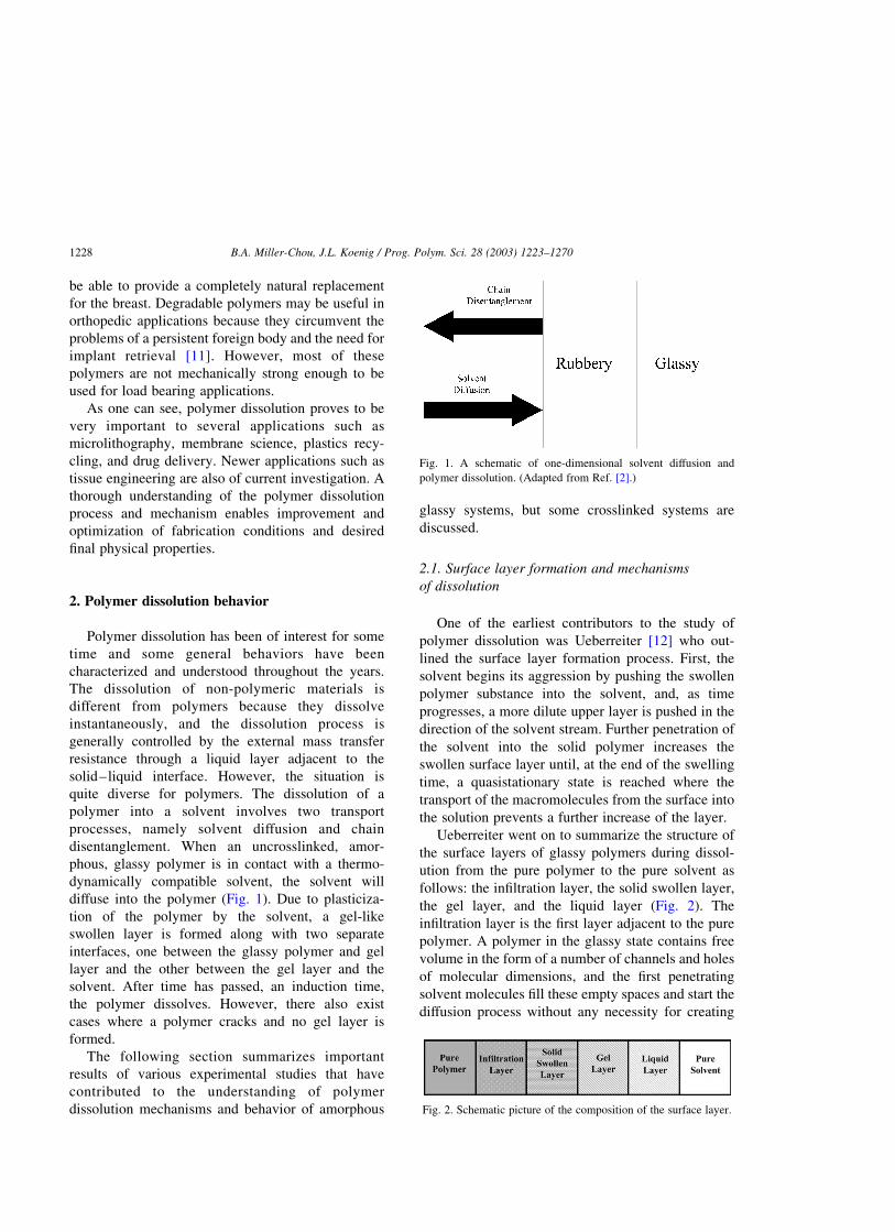
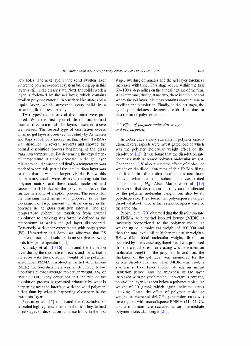
quite diverse for polymers. The dissolution of a

polymer into a solvent involves two transport

processes, namely solvent diffusion and chain

disentanglement. When an uncrosslinked, amor-

phous, glassy polymer is in contact with a thermo-

dynamically compatible solvent, the solvent will

diffuse into the polymer (Fig. 1). Due to plasticiza-

tion of the polymer by the solvent, a gel-like

swollen layer is formed along with two separate

interfaces, one between the glassy polymer and gel

layer and the other between the gel layer and the

solvent. After time has passed, an induction time,

the polymer dissolves. However, there also exist

cases where a polymer cracks and no gel layer is

formed.

The following section summarizes important

results of various experimental studies that have

contributed to the understanding of polymer

dissolution mechanisms and behavior of amorphous

glassy systems, but some crosslinked systems are

discussed.

2.1. Surface layer formation and mechanisms

of dissolution

One of the earliest contributors to the study of

polymer dissolution was Ueberreiter [12] who out-

lined the surface layer formation process. First, the

solvent begins its aggression by pushing the swollen

polymer substance into the solvent, and, as time

progresses, a more dilute upper layer is pushed in the

direction of the solvent stream. Further penetration of

the solvent into the solid polymer increases the

swollen surface layer until, at the end of the swelling

time, a quasistationary state is reached where the

transport of the macromolecules from the surface into

the solution prevents a further increase of the layer.

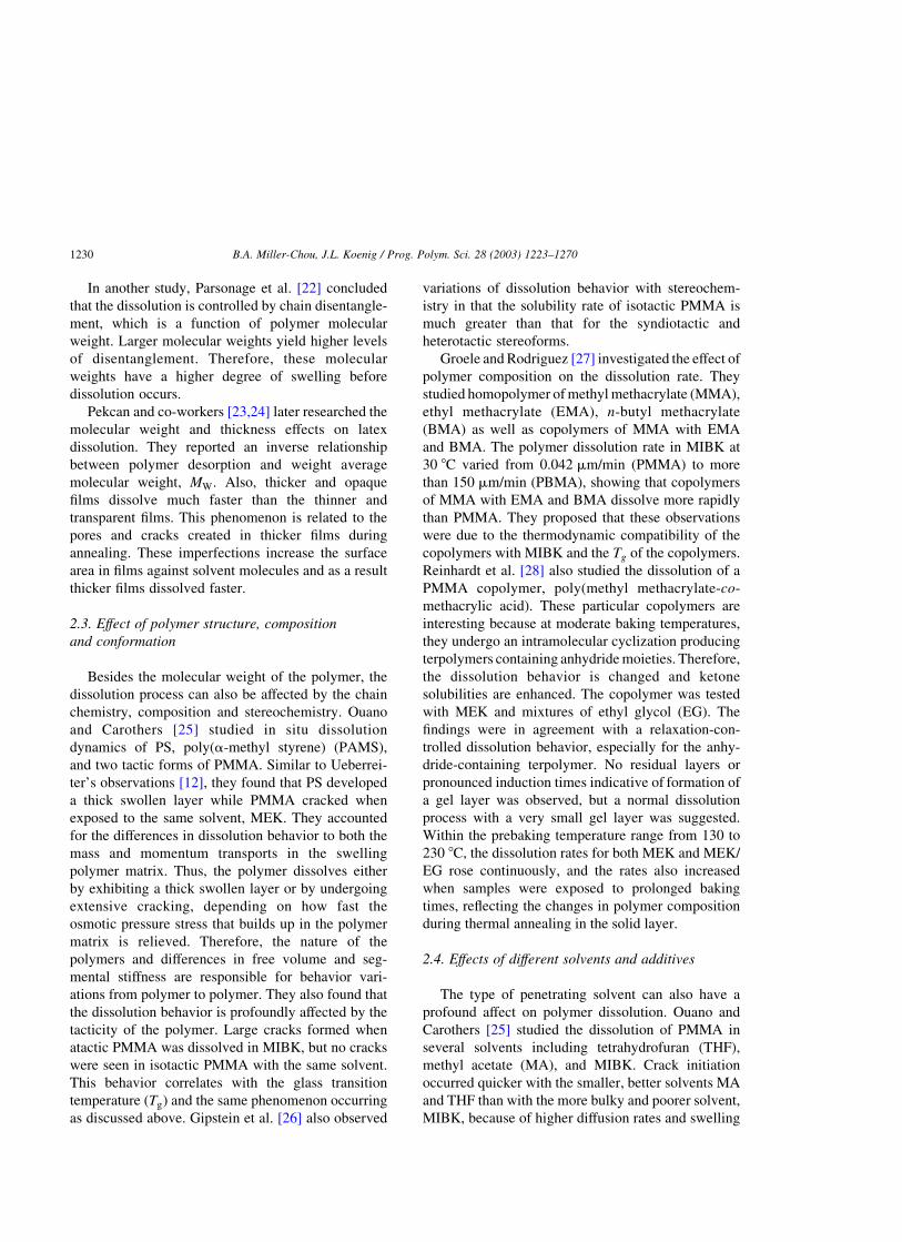
Ueberreiter went on to summarize the structure of

the surface layers of glassy polymers during dissol-

ution from the pure polymer to the pure solvent as

follows: the infiltration layer, the solid swollen layer,

the gel layer, and the liquid layer (Fig. 2). The

infiltration layer is the first layer adjacent to the pure

polymer. A polymer in the glassy state contains free

volume in the form of a number of channels and holes

of molecular dimensions, and the first penetrating

solvent molecules fill these empty spaces and start the

diffusion process without any necessity for creating

Fig. 1. A schematic of one-dimensional solvent diffusion and

polymer dissolution. (Adapted from Ref. [2].)

Fig. 2. Schematic picture of the composition of the surface layer.


new holes. The next layer is the solid swollen layer

where the polymer–solvent system building up in this

layer is still in the glassy state. Next, the solid swollen

layer is followed by the gel layer, which contains

swollen polymer material in a rubber-like state, and a

liquid layer, which surrounds every solid in a

streaming liquid, respectively.

Two types/mechanisms of dissolution were pro-

posed. With the first type of dissolution, termed

‘normal dissolution’, all the layers described above

are formed. The second type of dissolution occurs

when no gel layer is observed. In a study by Asmussen

and Raptis [13], poly(methyl methacrylate) (PMMA)

was dissolved in several solvents and showed the

normal dissolution process beginning at the glass

transition temperature. By decreasing the experimen-

tal temperature, a steady decrease in the gel layer

thickness could be seen until finally a temperature was

reached where this part of the total surface layer was

so thin that it was no longer visible. Below this

temperature, cracks were observed running into the

polymer matrix, and these cracks coalesced and

caused small blocks of the polymer to leave the

surface in a kind of eruption process. The reason for

the cracking mechanism was proposed to be the

freezing-in of large amounts of stress energy in the

polymer in the glass transition interval. The gel

temperature (where the transition from normal

dissolution to cracking) was formally defined as the

temperature at which the gel layer disappeared.

Conversely with other experiments with polystyrene

(PS), Ueberreiter and Asmussen observed that PS

underwent normal dissolution in most solvents owing

to its low gel temperature [14].

Krasicky et al. [15,16] monitored the transition

layer during the dissolution process and found that it

increases with the molecular weight of the polymer.

Also, when PMMA dissolved in methyl ethyl ketone

(MEK), the transition layer was not detectable below

a polymer number average molecular weight, MN; of

about 30 000. They concluded that the rate of the

dissolution process is governed primarily by what is

happening near the interface with the solid polymer,

rather than by what is happening elsewhere in the

transition layer.

Pekcan et al. [17] monitored the dissolution of

annealed high-Tg latex films in real time. They defined

three stages of dissolution for these films. In the first

stage, swelling dominates and the gel layer thickness

increases with time. This stage occurs within the first

60–100 s, depending on the annealing time of the film.

At a later time, during stage two, there is a time period

where the gel layer thickness remains constant due to

swelling and dissolution. Finally, in the last stage, the

gel layer thickness decreases with time due to

desorption of polymer chains.

2.2. Effect of polymer molecular weight

and polydispersity

In Ueberreiter’s early research in polymer dissol-

ution, several aspects were investigated, one of which

was the polymer molecular weight effect on the

dissolution [12]. It was found that the dissolution rate

decreases with increased polymer molecular weight.

Cooper et al. [18] also studied the effects of molecular

weight on the dissolution rates of thin PMMA films,

and found that dissolution results in a non-linear

behavior when the log dissolution rate was plotted

against the log MN: Also, Manjkow et al. [19]

discovered that dissolution not only can be affected

by the polymer molecular weight, but also by its

polydispersity. They found that polydisperse samples

dissolved about twice as fast as monodisperse ones of

the same MN:

Papanu et al. [20] observed that the dissolution rate

of PMMA with methyl isobutyl ketone (MIBK) is

inversely proportional to the polymer molecular

weight up to a molecular weight of 100 000 and

then the rate levels off at higher molecular weights.

Below this critical molecular weight, dissolution

occurred by stress cracking, therefore, it was proposed

that the critical stress for crazing was dependent on

molecular weight of the polymer. In addition, the

thickness of the gel layer was monitored for the

ketone dissolutions, and when MIBK was used, a

swollen surface layer formed during an initial

induction period, and the thickness of the layer

increased with polymer molecular weight. However,

no swollen layer was seen below a polymer molecular

weight of 105 g/mol, which again indicated stress

cracking. Later, the effect of polymer molecular

weight on methanol (MeOH) penetration rates was

investigated with monodisperse PMMA (21–27 8C),

and a minimum rate occurred at an intermediate

polymer molecular weight [21].


In another study, Parsonage et al. [22] concluded

that the dissolution is controlled by chain disentangle-

ment, which is a function of polymer molecular

weight. Larger molecular weights yield higher levels

of disentanglement. Therefore, these molecular

weights have a higher degree of swelling before

dissolution occurs.

Pekcan and co-workers [23,24] later researched the

molecular weight and thickness effects on latex

dissolution. They reported an inverse relationship

between polymer desorption and weight average

molecular weight, MW: Also, thicker and opaque

films dissolve much faster than the thinner and

transparent films. This phenomenon is related to the

pores and cracks created in thicker films during

annealing. These imperfections increase the surface

area in films against solvent molecules and as a result

thicker films dissolved faster.

2.3. Effect of polymer structure, composition

and conformation

Besides the molecular weight of the polymer, the

dissolution process can also be affected by the chain

chemistry, composition and stereochemistry. Ouano

and Carothers [25] studied in situ dissolution

dynamics of PS, poly(a-methyl styrene) (PAMS),

and two tactic forms of PMMA. Similar to Ueberrei-

ter’s observations [12], they found that PS developed

a thick swollen layer while PMMA cracked when

exposed to the same solvent, MEK. They accounted

for the differences in dissolution behavior to both the

mass and momentum transports in the swelling

polymer matrix. Thus, the polymer dissolves either

by exhibiting a thick swollen layer or by undergoing

extensive cracking, depending on how fast the

osmotic pressure stress that builds up in the polymer

matrix is relieved. Therefore, the nature of the

polymers and differences in free volume and seg-

mental stiffness are responsible for behavior vari-

ations from polymer to polymer. They also found that

the dissolution behavior is profoundly affected by the

tacticity of the polymer. Large cracks formed when

atactic PMMA was dissolved in MIBK, but no cracks

were seen in isotactic PMMA with the same solvent.

This behavior correlates with the glass transition

temperature ðTgÞ and the same phenomenon occurring

as discussed above. Gipstein et al. [26] also observed

variations of dissolution behavior with stereochem-

istry in that the solubility rate of isotactic PMMA is

much greater than that for the syndiotactic and

heterotactic stereoforms.

Groele and Rodriguez [27] investigated the effect of

polymer composition on the dissolution rate. They

studied homopolymer of methyl methacrylate (MMA),

ethyl methacrylate (EMA), n-butyl methacrylate

(BMA) as well as copolymers of MMA with EMA

and BMA. The polymer dissolution rate in MIBK at

30 8C varied from 0.042 mm/min (PMMA) to more

than 150 mm/min (PBMA), showing that copolymers

of MMA with EMA and BMA dissolve more rapidly

than PMMA. They proposed that these observations

were due to the thermodynamic compatibility of the

copolymers with MIBK and the Tg of the copolymers.

Reinhardt et al. [28] also studied the dissolution of a

PMMA copolymer, poly(methyl methacrylate-co-

methacrylic acid). These particular copolymers are

interesting because at moderate baking temperatures,

they undergo an intramolecular cyclization producing

terpolymers containing anhydride moieties. Therefore,

the dissolution behavior is changed and ketone

solubilities are enhanced. The copolymer was tested

with MEK and mixtures of ethyl glycol (EG). The

findings were in agreement with a relaxation-con-

trolled dissolution behavior, especially for the anhy-

dride-containing terpolymer. No residual layers or

pronounced induction times indicative of formation of

a gel layer was observed, but a normal dissolution

process with a very small gel layer was suggested.

Within the prebaking temperature range from 130 to

230 8C, the dissolution rates for both MEK and MEK/

EG rose continuously, and the rates also increased

when samples were exposed to prolonged baking

times, reflecting the changes in polymer composition

during thermal annealing in the solid layer.

2.4. Effects of different solvents and additives

The type of penetrating solvent can also have a

profound affect on polymer dissolution. Ouano and

Carothers [25] studied the dissolution of PMMA in

several solvents including tetrahydrofuran (THF),

methyl acetate (MA), and MIBK. Crack initiation

occurred quicker with the smaller, better solvents MA

and THF than with the more bulky and poorer solvent,

MIBK, because of higher diffusion rates and swelling


power of these solvent molecules. They concluded

that if the ‘internal pressure’ builds up faster than the

glassy matrix can relax through gradual swelling,

catastrophic fracture results. Also, they pointed out

that polymer morphology at the molecular level has a

strong influence on the kinematics of dissolution.

Ouano [29] investigated the effect of residual

solvent content on the dissolution kinetics of poly-

mers. In this study, the dissolution rate of PMMA,

cresol-formaldehyde resin (novolac), and a mixture of

novolac resin and adiazo-photoactive compound

(PAC) showed interesting results. First, a few percent

change in the solvent content meant several orders of

magnitude change in solubility rate. Therefore, the

dependence of the dissolution rate on the residual

solvent content is very strong, and the dissolution

rate-solvent content relationship can be interpreted in

terms of the free volume theory. Second, addition of

the PAC to the novolac resin decreased the residual

solvent content of the resists at any prebaking

temperature. For example, at 85 8C prebake, pure

resin contained ca. 14% solvent, while the resist or the

resist analog contained only ca. 9.5% by weight.

Lastly, a very rapid drying of PMMA at 160 8C

resulted in very fast dissolution rate. This rapid

evolution of the solvent leaves ‘extra free volume’ and

strain in the PMMA.

Cooper et al. [30] investigated PMMA dissolution

rates with mixed solvents. It was found that the

addition of small non-solvent molecules to a good

solvent results in a significant increase in the

dissolution rate of PMMA films. This enhancement

of the rate was proposed to be the result of

‘plasticization’ of the polymer films by the small,

rapidly diffusing non-solvent molecules. Those mol-

ecules found to exhibit this enhancement effect at

lower concentrations were water, methanol, and

ethanol. Higher alcohols only decreased the dissol-

ution rate of the films. It was also noted that high

concentrations of the non-solvent molecules caused

the films to swell appreciably. In addition, this

enhancement effect was found to be less significant

in lower molecular weight PMMA when compared

with higher molecular weights.

Mixed solvents were also studied by Manjkow et al.

[31]. Solvent/non-solvent binary mixtures of MEK

and isopropanol (MEK/IpOH) and MIBK and metha-

nol (MIBK/MeOH) were used. A sharp transition

between complete solubility and almost total

insolubility was observed in a narrow concentration

range near 50:50 (by volume) solvent/non-solvent for

both mixtures. In the insoluble regime, the polymer

swelled up to three times its initial thickness. At 50:50

MEK/IPA, a temperature decrease from 24.8 to

18.4 8C caused a change from complete dissolution

to combined swelling/dissolution behavior and ren-

dered the PMMA film only 68% soluble. For MEK/

IPA, penetration rates increased with increasing MEK

concentration. However, for the MIBK/MeOH, a

maximum rate occurred at 60:40 MIBK/MeOH.

Papanu et al. [20] studied the PMMA dissolution in

ketones, binary ketone/alcohol mixtures and hydro-

xyketones. They found that the dissolution rate

decreases with increasing solvent size, indicating

that dissolution rate is limited by the rate of which

solvent molecules penetrate. For binary mixtures of

acetone/isopropanol, a transition from swelling to

dissolution occurred near acetone volume fractions of

0.45–0.5. Acetol caused only swelling, whereas

diacetone alcohol dissolved the films at approximately

a quarter of the rate of MIBK. Later, the effects of

solvent size were also investigated [21]. Penetration

rates were strongly dependent on solvent molar

volume for methanol, ethanol, and isopropoanol, but

1-butanol and 2-pentanol had rates similar to

isopropanol. Some of the lower molecular weight

films cracked in MeOH (relatively low temperatures),

but with the same molecular weight samples, no

cracking was observed with isopropanol (at elevated

temperatures). Papanu et al. explained this phenom-

enon by the isopropanol molecules not penetrating as

easily as the smaller MeOH molecules, and at higher

temperatures, the polymer chains can relax more

readily. Both of these factors inhibit the buildup of

catastrophic stress levels, and cracking is suppressed

at higher polymer molecular weights. Gipstein et al.

[26] observed that in a homologous series of n-alkyl

acetate developer solvents, the molecular size of the

solvent has a greater effect on the solubility rate than

the molecular weight of the resist.

Mao and Feng [32] studied the dissolution process

of PS in concentrated cyclohexane, a theta solvent for

PS. They proposed a two-step process for dissolution

within this system. First, swelling of the polymer

below the u temperature corresponds to the gradual

dispersion of the side-chain phenyl groups which


are solvated by cyclohexane molecules; while

the complete dissolution above the u temperature

corresponds to the gradual dispersion of the main

chains at a molecular level. These dispersions reflect

the fact that cohesional interaction among side-chain-

phenyl rings or main chains are weakened by solvent

molecules, which shows the existence of the cohe-

sional entanglements among polymer chains.

Rodriguez et al. [33] made several contributions to

the study of polymers used as positive photoresists in

microlithographic applications. The found that plas-

ticization of PMMA by poly(ethylene oxide) (PEO) of

molecular weight 4000 changed the dissolution rate in

direct proportion to the amount of PEO added. With a

weight fraction of 0.2 PEO, the dissolution rate was

double that for PMMA alone.

Harland et al. [34] studied the swelling and

dissolution of polymer for pharmaceutical and con-

trolled release applications. They researched the

swelling and dissolution behavior of a system

containing a drug and polymer. The dissolution was

characterized by two distinct fronts: one separating

the solvent from the rubbery polymer and the second

separating the rubbery region from the glassy

polymer. The drug release had a t0:5 dependence

relation to a diffusional term and a t1 relation to a

dissolution term, and the drug release rate was

independent of time when the two fronts’ movements

were synchronized.

2.5. Effect of environmental parameters

and processing conditions

External parameters such as agitation and

temperature as well as radiation exposure can

influence the dissolution process. Ueberreiter [12]

found that the velocity of dissolution increases with

the agitation and stirring frequency of the solvent

due to a decrease of the thickness of the surface

layer, and the dissolution rate approaches a limiting

value if the pressure of the solvent against the

surface of the polymer is increased (at all

temperatures). Pekcan et al. also studied the effects

of agitation and found that with no agitation, the

solvent molecules penetrate the polymer, and a gel

layer forms. However, the gel layer decreases in

magnitude with time due to desorption of the

polymer chains. On the other hand, when agitation

is present, no gel layer is formed because it is

stripped off rapidly by the stirring process. In the

latter case, the sorption of solvent molecules is

immediately followed by desorption of the polymer

chains from the swollen gel layer.

Manjkow et al. [19] conducted an investigation of

the influence of processing and molecular parameters

on the dissolution of these PMMA films with MIBK.

They discovered that dissolution rates are highly

sensitive to the molecular weight distribution, soft-

bake cooling cycle, and dissolution temperature. The

apparent activation energy for the dissolution of

PMMA varied from 25 to 43 kcal/mol depending

upon softbake cooling rates and molecular weight

distribution. The dissolution rate of air quenched,

monodisperse samples was found to vary with the

molecular weight to the power of 20.98, but for

slowly cooled samples, this constant was 85% higher.

Rao et al. [35] studied the influence of the spatial

distribution of sensitizer on the dissolution mechan-

ism of diazonaphthoquinone resists. Their studies

demonstrated that the physical distribution of the PAC

in the diazonaphthoquinone resists plays a significant

role in the dissolution behavior of the films. For

example, as little as 30 A of PAC preferentially placed

at the surface of the film or embedded between two

polymer layers could cause significant induction

period in development.

Parsonage and co-workers [22,36] investigated the

properties of positive resists, both PMMA and its

copolymers, and the effects of irradiation on degra-

dation and sensitivity. They found that irradiation led

to a drastic decrease in the molecular weights of all

the homo- and copolymers studied. Planar and radial

dissolution studies were performed in pure MEK or

ethanol at 26 8C with PMMA and poly(methyl

methacrylate-co-maleic anhydride) P(MMA-co-

MAH). It was observed that the process of dissolution

is dependent on the structure of the polymer. The

initial stages of the dissolution mechanism consisted

entirely of the polymer swelling. Once the swelling

reached a critical point, the dissolution occurred and

the polymer chains disentangled from the bulk and

dissolved away. At this time, the two boundaries

(gel–liquid and polymer–gel) proceeded at the same

velocity.

Drummond et al. [37] studied the effects of

radiation. With samples of P(MMA-co-MAH) with


MEK, it was shown that the dissolution process is

a function of radiation dose, and the process started

with swelling of the glassy polymeric slab by water

which was followed by chain disentanglement and

dissolution. It was also observed that when the

swelling rate was greater than the dissolution rate,

the gel layer thickness increased linearly with the

square root of time, and, conversely, if the dissolution

rate was greater than the swelling rate, then the gel

thickness decreased with time.

3. Polymer solubility and solubility parameters

Solubility parameters are often used in industry

to predict compatibility of polymers, chemical

resistance, swelling of cured elastomers by sol-

vents, permeation rates of solvents, and even to

characterize the surfaces of pigments, fibers, and

fillers [38,39]. Moreover, the usefulness of poly-

mers in many technological applications is criti-

cally dependent on the solubility parameter, d; as

noted by Bicerano [40]. Some of these applications

are listed below.

(1) The removal of unreacted monomers, process

solvents, and other synthesis of processing by-

products, can both enhance the performance of

the polymer and overcome health-related or

environment-related objections to the use of

certain types of polymers.

(2) The Flory–Huggins solution theory uses d to

determine whether two polymers (A and B)

will be miscible by Eq. (1)

xAB ¼ ½VrefðdA 2 dBÞ2�=RT ð1Þ

The Flory–Huggins interaction parameter xAB

is a function of temperature ðTÞ; the mole

fraction of each polymer, and the degree of

polymerization. In this equation, Vref is an

appropriately chosen ‘reference volume’, often

taken to be 100 cm3/mol, and R is the gas

constant. The blend miscibility is assumed to

decrease with increasing xAB: If strong inter-

actions, e.g. hydrogen bonds, are present

between structural units on polymers A and

B, more elaborate versions of the Flory–

Huggins solution theory can be used [41].

(3) Environmental crazing and stress cracking are

dependent upon the solution and the diffusion

of environmental agents in the polymer, and

thus upon d [42,43]. These phenomena are

important in determining the length of time

that a polymer part can be useful for its

application.

(4) In some applications, the interaction of the

polymer with a specific ‘solvent’ and/or with

certain molecules carried by that solvent is not a

detrimental event, but an essential aspect of the

performance of the polymer. Reverse osmosis

membranes and swollen hydrogels used in

applications such as the desalination of water,

kidney dialysis, soft contact lenses and surgical

implants [44] are among such polymers.

(5) Plasticization is another area where the nature of

the interaction of a polymer with molecules is

critical to the usefulness of the polymer in many

applications. Sears and Darby [45] have reviewed

the importance of d in the role of polymer-

plasticizer compatibility for effective

plasticization.

The solubility parameter is important in the theory

of solutions and has been shown to be connected to

other physical properties such as surface tension [46]

and wettability [47–49], the ratio of the coefficient of

thermal expansion to compressibility [50], the boiling

points in the case of non-polar liquids [50], the

ultimate strength of materials [51], and the glass

transition temperature of polymers [52]. Therefore,

the ability to estimate the solubility parameters can

often be a useful tool to predicting systems’ physical

properties and performance.

It is the goal of this section to discuss the basis for

solubility parameters, their use in predicting polymer

dissolution, and the methods from which one can

obtain the solubility parameters for both polymers

(solute) and solvents.

3.1. Thermodynamics background

The solubility of a given polymer in various

solvents is largely determined by its chemical

structure. Polymers will dissolve in solvents whose

solubility parameters are not too different from their


own. This principle has become known as ‘like

dissolves like’, and, as a general rule, structural

similarity favors solubility.

Dissolution of an amorphous polymer in a solvent

is governed by the free energy of mixing [39]

DGm ¼ DHm 2 TDSm ð2Þ

where DGm is the Gibbs free energy change on mixing,

DHm is the enthalpy change on mixing, T is the

absolute temperature, and DSm is the entropy change

on mixing. A negative value of the free energy change

on mixing means that the mixing process will occur

spontaneously. Otherwise, two or more phases result

from the mixing process. Since the dissolution of a high

molecular weight polymer is always associated with a

very small positive entropy change, the enthalpy term

is the crucial factor in determining the sign of the Gibbs

free energy change. Solubility parameters were devel-

oped to describe the enthalpy of mixing [39].

Hildebrand pointed out that the order of solubility

of a given solute in a series of solvents is determined

by the internal pressures of the solvents [53]. Later,

Scatchard introduced the concept of ‘cohesive energy

density’ into Hildebrand’s theories [54]. Hildebrand

and Scott [50] and Scatchard [55] proposed that the

enthalpy of mixing is given by

DHm ¼ Vmix½ðDEV1 =V1Þ

1=2 2 ðDEV2 =V2Þ

1=2�2F1F2 ð3Þ

where Vmix is the volume of the mixture, DEVi is

the energy of vaporization of species i; Vi is the

molar volume of species i; and Fi is the volume

fraction of i in the mixture. DEVi is the energy

change upon isothermal vaporization of the

saturated liquid to the ideal gas state at infinite

volume [39].

The cohesive energy, E; of a material is the

increase in the internal energy per mole of the material

if all of the intermolecular forces are eliminated. The

cohesive energy density (CED) Eq. (4), is the energy

required to break all intermolecular physical links in a

unit volume of the material [40]

CED ¼ E=V ¼ ðDHvap 2 RTÞ=V ð4Þ

where DHvap is the enthalpy of vaporization.

The Hildebrand solubility parameter is defined as

the square root of the cohesive energy density:

d ¼ ðE=VÞ1=2 ð5Þ

Eq. (3) can be rewritten to give the heat of mixing

per unit volume for a binary mixture:

DHm=V ¼ ðd1 2 d2Þ2F1F2 ð6Þ

The heat of mixing must be smaller than the

entropic term in Eq. (2) for polymer – solvent

miscibility ðDGm # 0Þ: Therefore, the difference in

solubility parameters ðd1 2 d2Þ must be small for

miscibility or dissolution over the entire volume

fraction range [39]. However, these predictions with

the Hildebrand solubility parameters are made with

the absence of any specific interactions, especially

hydrogen bonds. They also do not account for the

effects of morphology (crystallinity) and cross-link-

ing. In addition, there may be (non-ideal) changes

with changes in temperature and, in many cases, with

changes in concentration.

One of the early schemes to overcome incon-

sistencies in the Hildebrand solubility parameter

introduced by hydrogen bonding was proposed by

Burrell [56], and is based on the assumption that

solubility is greatest between materials with similar

polarities. This method divided solvents into three

categories depending on the hydrogen bonding: poor,

moderate, and strong hydrogen bonding capabilities.

The system of Burrell is summarized as follows: weak

hydrogen bonding liquids are hydrocarbons, chlori-

nated hydrocarbons and nitrohydrocarbons; moderate

hydrogen bonding liquids are ketones, esters, ethers,

and glycol monoethers; and strong hydrogen bonding

liquids are alcohols, amines, acids, amides, and

aldehydes.

Hansen also accounted for molecular interactions

and developed solubility parameters based on three

specific interactions [38].

The first and most general type of interaction is the

‘non-polar’, also termed dispersive interactions, or

forces. These forces arise because each atom consists

of negatively charged electrons orbiting around a

central positively charged nucleus. The moving

negative charges create an electromagnetic field,

which attracts all atoms to one another regardless of

direction [57]. All molecules have this type of

attractive force.

Polar cohesive forces, the second type of

interaction, are produced by permanent dipole–

dipole interactions. These polar forces roughly

correlate with the dipole moment of the molecule


and the contribution to the dipole moment [40].

They are inherently molecular interactions and are

found in most molecules to one extent or another.

The third major interaction is hydrogen bonding.

Hydrogen bonding is a molecular interaction and

resembles the polar interactions. These bonds are

considerably weaker than covalent bonds but are

much stronger than ordinary dipole – dipole

interactions.

Therefore, as Hansen proposed, the cohesive

energy has three components, corresponding to the

three types of interactions:

E ¼ ED þ EP þ EH ð7Þ

Dividing the cohesive energy by the molar volume

gives the square of the Hildebrand solubility par-

ameter as the sum of the squares of the Hansen

dispersion (D), polar (P), and hydrogen bonding (H)

components:

E=V ¼ ED=V þ EP=V þ EH=V ð8Þ

d2 ¼ d2D þ d2

P þ d2H ð9Þ

3.2. Estimation of solubility parameters

For low molecular weight substances (solvents),

DHvap can be calculated by a number of methods.

Experimental values of DHvap can be obtained using

vapor pressure – temperature data or from heat

capacity-temperature measurements. Numerical

values for most solvents can be found in the literature.

Therefore, estimating values of d for low molecular

weight solvents can be made.

When values of DHvap are known at one

temperature, they can be converted to the appro-

priate DHvap values at any other temperature using

the following empirical relationship first proposed

by Watson [58,59]:

DHvap;T2=DHvap;T1

¼ ½ðTc 2 T2Þ=ðTc 2 T1Þ�0:38 ð10Þ

This equation is useful because many liquids’

DHvap values, corresponding only to the normal

boiling points, have been reported. Also, this

expression is fairly accurate because the predicted

DHvap values are usually within about 2% of the

experimental values [59].

Hildebrand developed another method to calculate

DHvap based on an empirical relationship which

relates DHvap at 25 8C to the normal boiling point,

Tb; of non-polar liquids [50]:

DHvap ¼ T2b þ 23:7Tb 2 2950 ð11Þ

The dD parameter can by calculated according to

the procedures outlined by Blanks and Prausnitz [60].

They used the idea of homomorphs to obtain

solubility parameters. For example, the homomorph

of a polar molecule is a non-polar molecule having

very nearly the same size and shape as that of the polar

molecule in question. This concept is relatively easy

to apply. The polar energy of vaporization is simply

the difference between the experimentally determined

total energy of vaporization and the energy of

vaporization of the homomorph at the same reduced

temperature [60]. Charts [61] can be used to find the

energy of vaporization or cohesive energy, depending

on whether the molecule of interest is aliphatic,

cycloaliphatic, or aromatic.

The critical temperature, Tc; is required to make

use of these charts. If the critical temperature cannot

be found, it must be estimated. The Tc values can be

calculated from the Lyderson constants ðPDT Þ

1;

provided the boiling point Tb at 1 atm is known, by

Tb=Tc ¼ 0:567 þX

DT 2X

DT

� �2ð12Þ

Blanks and Prausnitz calculated the polar solubility

parameters by splitting the energy of vaporization of

the polar fluid into non-polar and polar parts.

However, these ‘polar’ parameters were actually the

combined polar and hydrogen bonding parameters.

These values were reassigned by Hansen and Skaarup

[62] according to the Bottcher equation so that the real

polar solubility component could be calculated by the

equation

d2P ¼ ½12 108ð12 1Þðn2

l þ 2Þm2�=½V2ð21þ n2l Þ� ð13Þ

where m is the dipole moment (Debye), 1 is the

dielectric constant, and nl is the refractive index of the

liquid. Since most of these property constants are not

reported for many compounds, Hansen and Beer-

bower [63] devised a simpler equation

dP ¼ 37:4m=V1=2 ð14Þ


Until this point in time, the hydrogen bonding

parameter was almost always found by subtraction of

the polar and dispersion energies of vaporization from

the total energy of vaporization. However, now the

group contribution techniques are considered reason-

ably reliable for most of the required calculations and,

in fact, more reliable than estimating several of the

other parameters to ultimately arrive at the subtraction

step just mentioned [38]. These techniques will be

discussed later.

However, obtaining the solubility parameters for

high molecular weight materials (polymers) is

difficult because there is no measurable value of

DHvap or boiling point since polymers will degrade

before they vaporize. Therefore, indirect methods

must be used to obtain polymer solubility parameters,

and these can be based on various kinds of

measurements such as the determination of solubility

relationships, of thermal changes accompanying

mixing, and of various colligative properties such as

vapor pressure, depression of the freezing point, and

osmotic pressure. These measurements in conjunction

with suitable theory can be used to evaluate d for

polymers [43]. Some widely used methods are

1. Directly measuring the solubility in a range of

solvents or by measuring the degree of swelling of

lightly crosslinked polymers. The extent of swel-

ling will be a maximum when the d value of the

solvent matches that of the polymer.

2. Measuring the intrinsic viscosity of the uncros-

slinked polymer in a series of solvents. The d value

for the solvent which produces the highest

viscosity can be taken as the d for the polymer.

The best solvent gives the highest viscosity

because the polymer chain is fully expanded and

has the highest hydrodynamic volume.

However, these methods can be tedious and time

consuming, so several alternative methods of

calculation and calculating the values by group

contributions have been explored extensively.

3.3. Group contribution methods of calculation

of solubility parameters

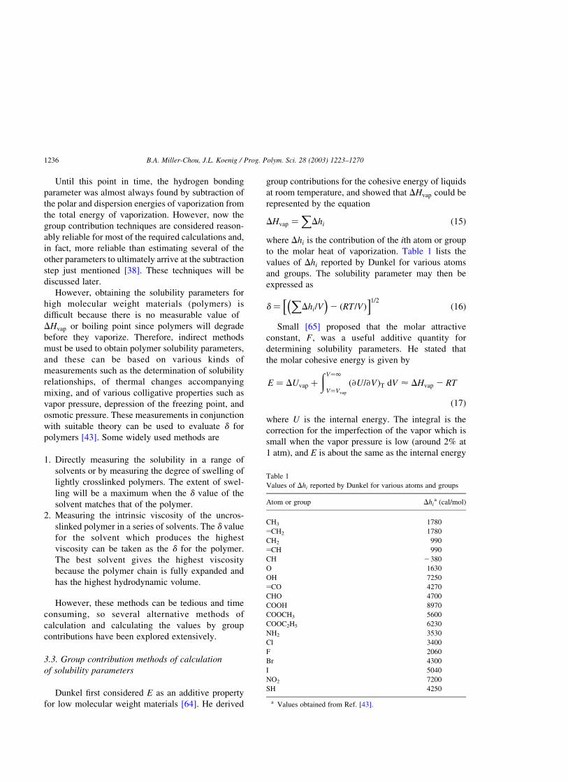
Dunkel first considered E as an additive property

for low molecular weight materials [64]. He derived

group contributions for the cohesive energy of liquids

at room temperature, and showed that DHvap could be

represented by the equation

DHvap ¼X

Dhi ð15Þ

where Dhi is the contribution of the ith atom or group

to the molar heat of vaporization. Table 1 lists the

values of Dhi reported by Dunkel for various atoms

and groups. The solubility parameter may then be

expressed as

d ¼X

Dhi=V� �

2 ðRT =VÞh i1=2

ð16Þ

Small [65] proposed that the molar attractive

constant, F; was a useful additive quantity for

determining solubility parameters. He stated that

the molar cohesive energy is given by

E ¼ DUvap þðV¼1

V¼Vvap

ð›U=›VÞT dV < DHvap 2 RT

ð17Þ

where U is the internal energy. The integral is the

correction for the imperfection of the vapor which is

small when the vapor pressure is low (around 2% at

1 atm), and E is about the same as the internal energy

Table 1

Values of Dhi reported by Dunkel for various atoms and groups

Atom or group Dhia (cal/mol)

CH3 1780

yCH2 1780

CH2 990

yCH 990

CH 2380

O 1630

OH 7250

yCO 4270

CHO 4700

COOH 8970

COOCH3 5600

COOC2H5 6230

NH2 3530

Cl 3400

F 2060

Br 4300

I 5040

NO2 7200

SH 4250

a Values obtained from Ref. [43].


of vaporization. Since Scatchard [55] showed by the

equation

E1=2ðn1V1 þ n2V2Þ1=2 ¼ n1ðE1V1Þ

1=2 þ n2ðE2V2Þ1=2

ð18Þ

that ðEVÞ1=2 is an additive property, Small considered

it reasonable that it might add, in compounds, on an

atomic and constitutive basis. It proved possible to

find a set of additive constants for the common

groups of organic molecules, which would allow

the calculation of ðEVÞ1=2: Therefore, for one mole of

the substance concerned,P

F summed over the groups

present in the molecule of the substance gives the

value of ðEVÞ1=2: Then

E ¼X

F� �2

=V ð19Þ

CED ¼X

F=V� �2

ð20Þ

d ¼X

F=V ð21Þ

Table 2 lists Small’s molar attraction constants for

several common functional groups or organic com-

pounds, and Table 3 gives some values of the

solubility parameters (for polymers) calculated from

those constants in Table 2. These values were

determined with the assumption that for the classes

of compounds considered the dipole-interaction

energy was negligible.

Rheineck and Lin [66] also developed another

system of additive group increments and found that

for homologous series of low molecular weight

liquids, the contribution to the cohesive energy of

the methylene group was not constant, but depended

on the values of other structural groups in the

molecule.

Hoy [67] combined vapor pressure data and group

contributions to calculate the solubility parameters of

a broad spectrum of solvents and chemical. His

technique is as follows. First, the heat of vaporization

at a given temperature from available vapor pressure

data is given by the following Haggenmacher [68]

equations

PðVg 2 VlÞ ¼ ðRT =MÞ½1 2 ðPT3c Þ=ðPcT3Þ�1=2 ð22Þ

DH ¼ ðdP=dtÞðRT2=MPÞ½1 2 ðPT3

c Þ=ðPcT3Þ�1=2 ð23Þ

Table 2

Small’s molar attraction constants for several common functional

groups or organic compounds

Atom

or group

Fp (at 25 8C)a

cal1/2 c.c.1/2

Atom

or group

Fp

(at 25 8C)a

cal1/2 c.c.1/2

CH3 214 CO ketones 275

CH2 133 COO esters 310

28 CN 410

293 Cl (mean) 260

yCH2 190 Cl single 270

–CHy 111 Cl twinned

as in sCCl2

260

sCy 19 Cl triple

as in –CCl3

250

CHxC– 285 Br single 340

–CxC– 222 I single 425

Phenyl 735 CF2 n-fluoro-

carbons only

150

Phenylene

ðo;m; pÞ

658 CF3 n-fluoro-

carbons only

274

Naphthyl 1146 S sulphides 225

Ring, 5-membered 105–115 SH thiols 315

Ring, 6-membered 95–105 O·NO2 nitrates ,440

Conjugation 20–30 NO2 (aliphatic

nitro-compounds)

,440

H (variable) 80–100 PO4 (organic

phosphates)

,500

O ethers 70


Table 3

Values of the solubility parameters (for polymers) calculated from

those constants in Table 2

Polymer dðcalcÞa

Polytetrafluoroethylene 6.2

Polyisobutylene 7.7

Natural rubber 8.15

Polybutadiene 8.38

Polystyrene 9.12

Neoprene GN 9.38

Polyvinyl acetate 9.4

Polyvinyl chloride 9.55

Polyacrylonitrile 12.75

Polymethyl methacrylate 9.25



where Vg is the specific volume of the gas phase, Vl is

the specific volume of the liquid phase, M is the

molecular weight, P is the pressure, and Pc is the

critical pressure. Using these equations and the vapor

pressure in the form of the Antoine equation

log P ¼ ½2B=ðT þ CÞ� þ A ð24Þ

where P is in mm Hg, T is in 8C, and A;B; and C are

constants, the solubility parameter can then be

calculated by the equation

d ¼ {ðRTr=MÞ½1 2 ðPT3c Þ=ðPcT3Þ�1=2

½ð2:303BT2Þ=ðT þ C 2 273:16Þ2�2 1}1=2 ð25Þ

where r is density. However, the temperature of

interest (usually 25 8C) can be beyond the range of the

usual Antoine expression. This problem can be

overcome by an alternate means of estimating the

heat of vaporization at room temperature from data at

different temperatures. At low pressures below

atmospheric pressure the latent heat of vaporization

follows the relationship:

log DHvap ¼ ð2m=2:303Þt þ log DH0vap ð26Þ

where DH0vap is the heat of vaporization at some

standard temperature and m is a constant. Using this

relationship it is possible to estimate DHvap at 25 8C

by calculating the heat of vaporization in the

temperature range in which the Antoine constants

are valid and fitting these values into Eq. (26) to

determine the slope m; and DH0vap:

Hoy also re-examined Small’s molar attraction

constants using regression analysis, making correc-

tions for acids, alcohol, and other compounds which

are capable of association. Hoy assumed that

carboxylic acids, for example, exist as dimers. Then

the solubility parameter can be expressed as

d ¼ ðDUr=MÞ1=2 ð27Þ

but for the case of dimeric carboxylic acids the actual

molecular weight is twice that of the original and the

solubility parameter becomes

d ¼ ðDUr=MÞ1=2 £ ðp

2Þ=2 ð28Þ

E was calculated using the group contributions of

Fedors [43] who found that a general system for

estimating both DEVi and V could be set up simply by

assuming

DEVi ¼

XDei ð29Þ

and

V ¼X

Dvi ð30Þ

where Dei and Dvi are the additive atomic and group

contributions for the energy of vaporization and molar

volume, respectively. In addition, it was found that

both DEVi and V for cyclic compounds could be

estimated from the properties of linear compounds

having the same chemical structure by adding a

cyclization increment to both DEVi and V of the linear

compound.

However, a problem with the Fedors method arises

when the substance has either a Tg or Tm above room

temperature because the estimates of both V and d

refer to the supercooled liquid rather than to the glass

or to the crystalline phase. V values are smaller and

DEVi values are greater than experimental values.

Therefore, small correction factors are introduced to

alleviate this problem. For high molecular weight

polymers with Tgs in this range, these correction

factors are

Dvi ¼ 4n; n , 3 ð31Þ

Dvi ¼ 2n; n # 3 ð32Þ

where n is the number of main chain skeletal atoms

(including those in a ring system that is part of the

chain’s backbone) in the smallest repeating unit of the

polymer. When polymers with Tms above room

temperature are concerned, the relationship between

the molar volume of the liquid and crystalline phase,

Vc; can be taken as

V ¼ ð1 þ 0:13XÞVc ð33Þ

where X is the degree of crystallization. Fedors noted

that since the estimates of DEVi for a glass did not vary

appreciably from that calculated for the liquid, one

could assume that the DEVi for the glass and liquid

were the same.

Using Eqs. (29) and (30)

d ¼X

Dei=X

Dvi

� �1=2ð34Þ

and the limiting form for high molecular weight

liquids becomes


d ¼X

Deir=X

Dvir

� �1=2ð35Þ

Hoftzyer and Van Krevelen [69] compiled a set of

group contribution values based on atomic contri-

butions to calculate F derived by Van Krevelen [70]

and E calculations based on Small’s method. Their

method estimates the individual solubility parameter

components from group contributions using the

following equations:

dD ¼X

FDi=V ð36Þ

dP ¼X

F2Pi

� �1=2=V ð37Þ

dH ¼X

EHi=V� �1=2

ð38Þ

These parameters are then incorporated into Eq. (9)

to calculate the Hildebrand parameter.

The prediction of dD is the same type of formula

used as Small first proposed for the prediction of the

total solubility parameter, d: The group contributions

FDi to the dispersion component FD of the molar

attraction constant can simply be added. The same

method holds for dP as long as only one polar group

is present. To correct for the interaction of polar

groups within a molecule, the form of Eq. (37) has

been chosen. The polar component is further

reduced, if two identical polar groups are present

in a symmetrical position. To take this effect into

account, the value of dP; calculated with Eq. (37)

must be multiplied by a symmetry factor of 0.5 for

one plane of symmetry, 0.25 for two planes of

symmetry, or 0 for more planes of symmetry. The F-

method is not applicable to the calculation of dH:

Hansen stated that the hydrogen bonding energy EHi

per structural group is approximately constant,

which leads to the form of Eq. (38). For molecules

with several planes of symmetry, dH ¼ 0 [68].

3.4. The x parameter and its relation to Hansen

solubility parameters

The Flory–Huggins parameter, x; has been used

for many years in connection with polymer solution

behavior, but it is desirable to relate this parameter

to the Hansen solubility parameters (HSP). x is

an adjustable parameter that can be obtained from

experimental measurements (e.g. from osmotic press-

ure measurement), but if the solubility parameters of

the system are known, they can be used to estimate x

as follows

xsp ¼ 0:34 þ Vs=RTðds 2 dpÞ ð39Þ

The 0.34 is a factor which is necessary to preserve

the Flory form of the chemical potential expression.

The most likely origin of this correction term lies in

so-called free volume effects that are neglected in the

Flory–Huggins treatment. In the liquid state, the

motion and vibrations of the molecules lead to density

fluctuations, or free volume. The free volume

associated with a low molecular weight liquid is

usually larger than that of a polymer so that in

mixtures of the two there is a mismatch of free

volumes. This leads to the need for an additional term.

In fact, a more general way of expressing the Flory x

term is to let it have the form:

x ¼ a þ b=T ð40Þ

where the quantity a can be thought of as an entropic

component of x; accounting for non-combinatorial

entropy changes such as those associated with free

volume, while b is the enthalpic part [71].

3.5. Techniques to estimate Hansen solubility

parameters for polymers

For low molecular weight, non-polymeric sub-

stances, DHvap can be calculated by a number of

methods or easily found in the literature and hand-

books, so estimation of d is simple. However, this is

not the case for macromolecules. Polymers do not

vaporize so there is no real value of DHvap and d

becomes difficult to determine. Therefore, experimen-

tal methods to determine the HSP have been

developed.

The simplest method is to evaluate whether or not

the polymer dissolves in selective solvents, or

evaluate their solubility or degree of swelling/uptake

in a series of well-defined solvents [38]. The solvents

should have different HSP chosen for systematic

exploration of the three parameters at all levels. The

middle of the solubility range (in terms of ds) or the

maximum of swelling is taken as the dp:


Another solubility characterization method is that of

using the intrinsic viscosity. The intrinsic viscosities will

behigher inbetter solventsbecauseofgreater interactions

and greater polymer chain extensions (viscosity /

hydrodynamic volume of the chain in solution). The ds

of the solvent which gives the maximum dilute solution

viscosity is taken as the dp of the polymer.

There are other more complicated techniques to

evaluate polymer solubility parameters such as

permeation measurements, chemical resistance deter-

minations of various kinds, and surface attack. These

usefulness and accuracy of experimental techniques

depends on the polymer involved. Others can be

problematic because of the probable influence of

factors such as solvent molar volume and length of

time before attainment of equilibrium [38].

3.6. Predicting polymer solubility

Solubility behavior cannot be accurately predicted

by only the Hildebrand solubility parameter. As

mentioned earlier, solubility can be affected by any

specific interactions, especially H-bonds, polymer

morphology (crystallinity) and cross-linking, tem-

perature, and changes in temperature. Also of

importance is the size and shape of the solvent

molecules. Therefore, several graphing and modeling

techniques have been developed to aid in the

prediction of polymer solubility [72].

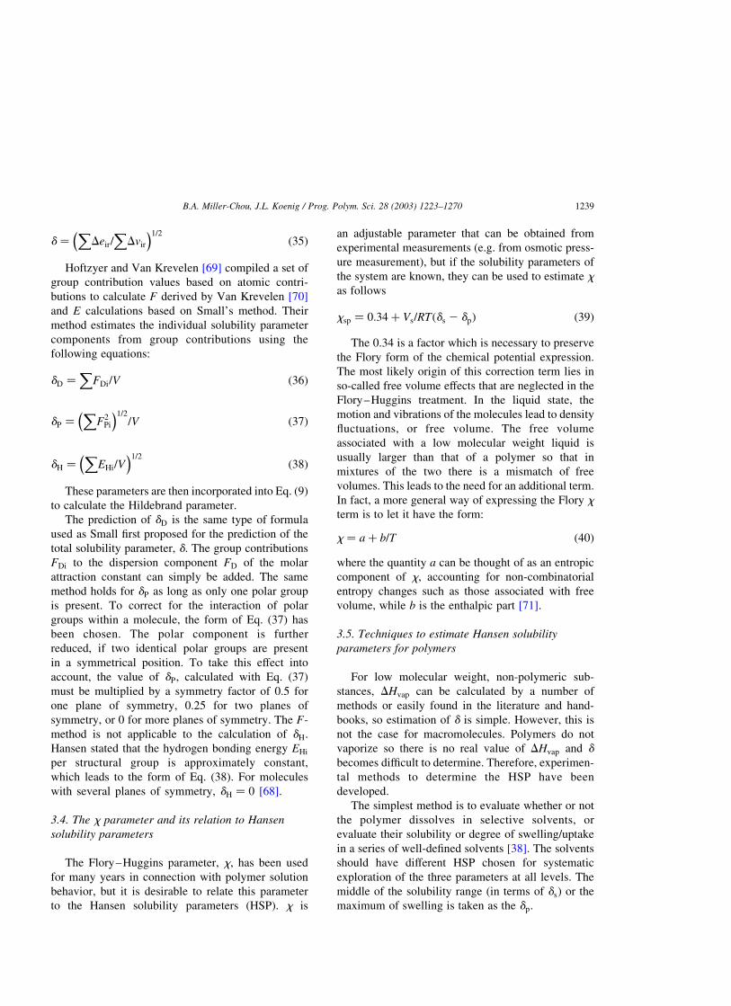
Crowley et al. [73] developed the first three-

component graphing system using the Hildebrand

parameter, a hydrogen bonding number, and the dipole

moment. A scale representing each of these three

values is assigned to a separate edge of a large empty

cube. Then, any point within the cube represents the

intersection of three specific values: the Hildebrand

value, dipole moment, and hydrogen bonding value

(Fig. 3) [72]. Once all the solvent positions are

determined, solubility tests are performed on poly-

mers. The positions of solvents that dissolve a polymer

are indicated by black balls, non-solvents by white

balls, and partial solubilities by gray balls. Therefore, a

three-dimensional volume of solubility is outlined with

liquids within the volume being active solvents and

liquids outside the volume being non-solvents. The

gray balls create the interface. The 3D plot can then be

translated into a 2D plot (Fig. 4) [72,74] by plotting the

data on a rectangular graph that represents only two of

the three component parameter scales. The polymer

solubility volume becomes an area which represents

either a single slice through the volume at a specified

value on the third component parameter scale or a

topographic map that indicates several values of the

third parameter at the same time.

Fig. 3. A three-dimensional box used to plot solubility information by Crowley, Teague, and Lowe with axes representing the Hildebrand

solubility parameter, d; the dipole moment, m; and hydrogen bonding value, h: (Adapted from Refs. [71,72].)


A second modeling technique of 3D solubility was

developed by Hansen [38,75]. The Hansen character-

ization is usually considered as a sphere. The center of

the sphere has the dD; dP; and dH values of the

polymer in question (solute). The radius of the sphere,

Ro; is termed the interaction radius. The boundary of

the spherical characterization is based on the require-

ment that ‘good’ solvents have a distance from the

center of the sphere, Ra (also termed the solubility

parameter distance) less than Ro: Ra is given by the

relation

R2a ¼ 4ðdD;p 2dD;sÞ

2 þðdP;p 2dP;sÞ2 þðdH;p 2dH;sÞ

2

ð41Þ

where dD;p; dP;p; and dH;p are the Hansen solubility

components for the polymer, and dD;s; dP;s; and dH;s

are the Hansen solubility components for the solvent.

Eq. (41) was developed from plots of experimental

data where the constant ‘4’ was found convenient and

correctly represented the solubility data as a sphere

encompassing the good solvent. This constant is

theoretically predicted corresponding states theory of

polymer solutions by the Prigogine when the

geometric mean is used to estimate the interaction in

mixtures of dissimilar molecules [38,76]. A con-

venient single parameter to describe solvent quality is

the relative energy difference, RED, number:

RED ¼ Ra=Ro ð42Þ

An RED number of 0 is found for no energy

difference. RED numbers less than 1.0 indicate high

affinity; RED equal to or close to 1.0 is a boundary

condition; and progressively higher RED numbers

indicate progressively lower affinities [38]. Fig. 5 is a

sketch of a sphere of solubility in the Hansen three-

dimensional solubility parameter system [75].

The Hansen characterization can also be rep-

resented in two dimensions by plotting a cross-section

through the center of the solubility sphere on a graph

that used only two of the three parameters, if need be.

Fig. 4. Approximate 2D representations of solid model and

solubility map for cellulose acetate. (Adapted from Refs. [71,73].)

Fig. 5. Sketch of a sphere of solubility in the Hansen three-dimensional solubility parameter system. (Adapted from Ref. [74].)


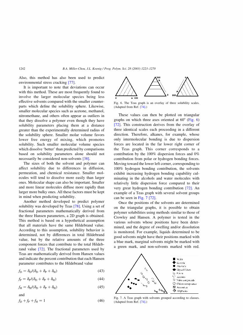
Also, this method has also been used to predict

environmental stress cracking [77].

It is important to note that deviations can occur

with this method. These are most frequently found to

involve the larger molecular species being less

effective solvents compared with the smaller counter-

parts which define the solubility sphere. Likewise,

smaller molecular species such as acetone, methanol,

nitromethane, and others often appear as outliers in

that they dissolve a polymer even though they have

solubility parameters placing them at a distance

greater than the experimentally determined radius of

the solubility sphere. Smaller molar volume favors

lower free energy of mixing, which promotes

solubility. Such smaller molecular volume species

which dissolve ‘better’ than predicted by comparisons

based on solubility parameters alone should not

necessarily be considered non-solvents [38].

The sizes of both the solvent and polymer can

affect solubility due to differences in diffusion,

permeation, and chemical resistance. Smaller mol-

ecules will tend to dissolve more easily than larger

ones. Molecular shape can also be important. Smaller

and more linear molecules diffuse more rapidly than

larger more bulky ones. All these factors must be kept

in mind when predicting solubility.

Another method developed to predict polymer

solubility was developed by Teas [78]. Using a set of

fractional parameters mathematically derived from

the three Hansen parameters, a 2D graph is obtained.

This method is based on a hypothetical assumption

that all materials have the same Hildebrand value.

According to this assumption, solubility behavior is

determined, not by differences in total Hildebrand

value, but by the relative amounts of the three

component forces that contribute to the total Hildeb-

rand value [72]. The fractional parameters used by

Teas are mathematically derived from Hansen values

and indicate the percent contribution that each Hansen

parameter contributes to the Hildebrand value

fD ¼ dD=ðdD þ dP þ dHÞ ð43Þ

fP ¼ dP=ðdD þ dP þ dHÞ ð44Þ

fH ¼ dH=ðdD þ dP þ dHÞ ð45Þ

and

fD þ fP þ fH ¼ 1 ð46Þ

These values can then be plotted on triangular

graphs on which three axes oriented at 608 (Fig. 6)

[72]. This construction derives from the overlay of

three identical scales each proceeding in a different

direction. Therefore, alkanes, for example, whose

only intermolecular bonding is due to dispersion

forces are located in the far lower right corner of

the Teas graph. This corner corresponds to a

contribution by the 100% dispersion forces and 0%

contribution from polar or hydrogen bonding forces.

Moving toward the lower left corner, corresponding to

100% hydrogen bonding contribution, the solvents

exhibit increasing hydrogen bonding capability cul-

minating in the alcohols and water molecules with

relatively little dispersion force compared to their

very great hydrogen bonding contribution [72]. An

example of a Teas graph with several solvent groups

can be seen in Fig. 7 [72].

Once the positions of the solvents are determined

on the triangular graphs, it is possible to obtain

polymer solubilities using methods similar to those of

Crowley and Hansen. A polymer is tested in the

various solvents whose positions have been deter-

mined, and the degree of swelling and/or dissolution

is monitored. For example, liquids determined to be

good solvents might have their positions marked with

a blue mark, marginal solvents might be marked with

a green mark, and non-solvents marked with red.

Fig. 6. The Teas graph is an overlay of three solubility scales.

(Adapted from Ref. [74].)

Fig. 7. A Teas graph with solvents grouped according to classes.



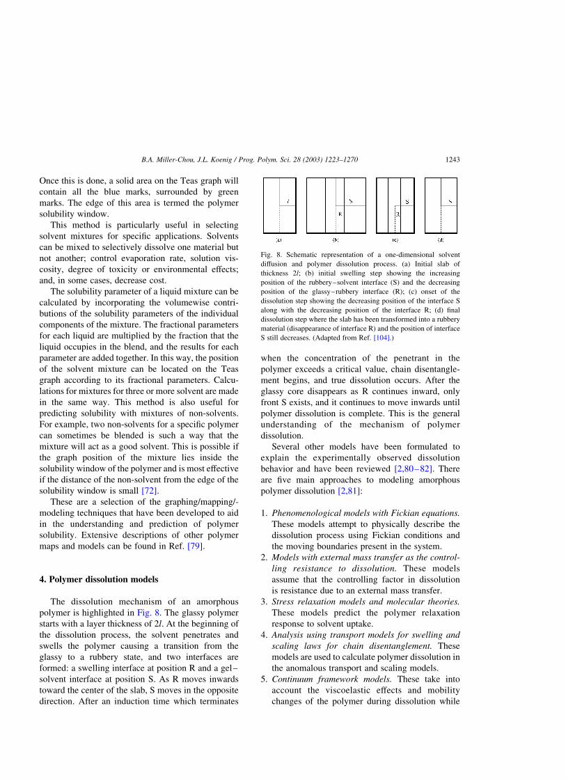
Once this is done, a solid area on the Teas graph will

contain all the blue marks, surrounded by green

marks. The edge of this area is termed the polymer

solubility window.

This method is particularly useful in selecting

solvent mixtures for specific applications. Solvents

can be mixed to selectively dissolve one material but

not another; control evaporation rate, solution vis-

cosity, degree of toxicity or environmental effects;

and, in some cases, decrease cost.

The solubility parameter of a liquid mixture can be

calculated by incorporating the volumewise contri-

butions of the solubility parameters of the individual

components of the mixture. The fractional parameters

for each liquid are multiplied by the fraction that the

liquid occupies in the blend, and the results for each

parameter are added together. In this way, the position

of the solvent mixture can be located on the Teas

graph according to its fractional parameters. Calcu-

lations for mixtures for three or more solvent are made

in the same way. This method is also useful for

predicting solubility with mixtures of non-solvents.

For example, two non-solvents for a specific polymer

can sometimes be blended is such a way that the

mixture will act as a good solvent. This is possible if

the graph position of the mixture lies inside the

solubility window of the polymer and is most effective

if the distance of the non-solvent from the edge of the

solubility window is small [72].

These are a selection of the graphing/mapping/-

modeling techniques that have been developed to aid

in the understanding and prediction of polymer

solubility. Extensive descriptions of other polymer

maps and models can be found in Ref. [79].

4. Polymer dissolution models

The dissolution mechanism of an amorphous

polymer is highlighted in Fig. 8. The glassy polymer

starts with a layer thickness of 2l: At the beginning of

the dissolution process, the solvent penetrates and

swells the polymer causing a transition from the

glassy to a rubbery state, and two interfaces are

formed: a swelling interface at position R and a gel–

solvent interface at position S. As R moves inwards

toward the center of the slab, S moves in the opposite

direction. After an induction time which terminates

when the concentration of the penetrant in the

polymer exceeds a critical value, chain disentangle-

ment begins, and true dissolution occurs. After the

glassy core disappears as R continues inward, only

front S exists, and it continues to move inwards until

polymer dissolution is complete. This is the general

understanding of the mechanism of polymer

dissolution.

Several other models have been formulated to

explain the experimentally observed dissolution

behavior and have been reviewed [2,80–82]. There

are five main approaches to modeling amorphous

polymer dissolution [2,81]:

1. Phenomenological models with Fickian equations.

These models attempt to physically describe the

dissolution process using Fickian conditions and

the moving boundaries present in the system.

2. Models with external mass transfer as the control-

ling resistance to dissolution. These models

assume that the controlling factor in dissolution

is resistance due to an external mass transfer.

3. Stress relaxation models and molecular theories.

These models predict the polymer relaxation

response to solvent uptake.

4. Analysis using transport models for swelling and

scaling laws for chain disentanglement. These

models are used to calculate polymer dissolution in

the anomalous transport and scaling models.

5. Continuum framework models. These take into

account the viscoelastic effects and mobility

changes of the polymer during dissolution while

Fig. 8. Schematic representation of a one-dimensional solvent

diffusion and polymer dissolution process. (a) Initial slab of

thickness 2l; (b) initial swelling step showing the increasing

position of the rubbery–solvent interface (S) and the decreasing

position of the glassy–rubbery interface (R); (c) onset of the

dissolution step showing the decreasing position of the interface S

along with the decreasing position of the interface R; (d) final

dissolution step where the slab has been transformed into a rubbery

material (disappearance of interface R) and the position of interface

S still decreases. (Adapted from Ref. [104].)


using anomalous transport models to predict the

behavior of solvent diffusion.

This section concentrates on several proposed

models of glassy polymer dissolution and is divided

into subsections based on the five classifications of

these models. A few selected examples of controlled

release models as also discussed, but a complete, more

detailed discussion of these systems is discussed

elsewhere [80].

4.1. Phenomenological models

4.1.1. The multi-phase Stefan problem

Tu and Ouano [83] proposed one of the first models

for polymer dissolution, assuming Fickian solvent

diffusion into the polymer followed by the establish-

ment of two distinct boundaries characterized by

sharp changes in the concentration of the solvent.

They also assumed that the conditions of constant

chain disassociation concentration and rate are

established immediately upon wetting the polymer

surface and that the solvent and the polymer are

incompressible. The first boundary between the liquid

solvent and gel-like solution phase provides a

partition between the dissolved and undissolved

polymer, and the concentration at this interface is a

defined quantity for a given polymer–solvent pair. At

the liquid–gel interface, the polymer molecules go

from the gel-like phase (entangled state) to a less

viscous liquid solution (free state) at a rate defined as

the disassociation rate, Rd; which may be experimen-

tally estimated by extrapolating the solubility rate to

very high solvent velocity across the liquid–gel

interface. The second boundary (also characterized

by concentration) lies between the gel-like and the

glass-like phases and is also marked by a change in the

diffusion coefficient of the solvent in the polymer

matrix. Once the concentrations at these interfaces are

defined and the different material parameters such as

the diffusion coefficients of the solvent and polymer

and Rd are known, the kinematics of dissolution can

be formulated and the spatial locations of the liquid–

gel and polymer–glass interfaces tracked with time.

Therefore, assuming the model is correct and the

parameters used are accurate, the kinematics of the

swelling and the dissolution of the polymer can be

described analytically.

It was proposed that the dissolution process is

disassociation-controlled if the polymer diffusion rate

in a liquid layer adjacent to the polymer–gel interface

is faster than the disassociation rate, or diffusion-

controlled if the diffusion rate is slower than the

disassociation rate. The solvent diffusional flux, js; is

defined by the diffusion coefficient of the solvent, Ds;

a function of fp; fsðfpÞ; and the position of the

solvent–gel interface, SðtÞ; as follows:

x , SðtÞ; js ¼ 2DsfsðfpÞð›fs=›xÞ ð47Þ

As the solvent penetrates the polymer, the polymer

swells at a rate,

vs ¼ 2jsðx; tÞ ð48Þ

and the interface position is derived as

dS=dt ¼ vs 2 Rd ð49Þ

The swelling velocity is equal in magnitude but

opposite in direction to the solvent flux, forming the

two interfaces. The flux of polymer, jp; at the gel–

liquid interface is dependent on the movement of that

interface and defined as

x . SðtÞ; jp ¼ 2DpfpðfpÞð›fp=›xÞ ð50Þ

The disassociation rate, Rd; is assumed to be equal

to the diffusion of the dissolved polymer into the bulk

liquid, i.e.

Rd ¼ jpðx; tÞ ð51Þ

As a result, the governing solvent diffusion

equation in the polymer in the region between the

solvent–gel interface, S; and the external polymer

thickness, L; is

S , x , L;

›fp=›t ¼ Ds ›=›x½fsðfpÞfp ›fp=›x�

ð52Þ

The governing polymer diffusion equation in the

liquid boundary layer is derived as

x , SðtÞ;

›fp=›t þ dS=dt ›fp=›x ¼ Dp ›=›x½fsðfpÞ›fp=›x�

ð53Þ

The equation for the interface position, S, is

dS=dt ¼ DpfpðfpÞ›fp=›x 2 DsfsðfpÞ›fs=›x ð54Þ


It is assumed that at small times, the solvent flux

into the polymer is sufficient to carry away all the

chains that dissolved from the gel into the liquid, and

the dissolution is disassociation-controlled. When the

solvent concentration at the gel–liquid boundary

reaches a constant concentration, the flux is no longer

sufficient to carry all of the dissolved chains away

from the surface, at which time the dissolution

becomes diffusion-controlled.

From existing data for the dissolution of PS in

MEK, this mathematical model was verified exper-

imentally by an in situ technique measuring the

motions of the polymer–gel and the liquid–gel

interfaces. Different forms of the functions fs and fpwere used in the simulations, and it was shown that

the concentration dependence of the diffusion coeffi-

cient is crucial. The disassociation rate, Rd; was

treated as a model parameter, and the simulations

failed to yield more insight into the actual rate.

Another weakness of the model is that no mechanism

for the disassociation of the polymer from gel is

provided. In addition, the contribution of reptation

time to the delay in the onset of dissolution is

neglected, and the assumption of constant solvent

concentration at the gel–liquid interface disregards

the possible effects of solvent history on the

dissolution process.

4.1.2. Disengagement dynamics

Devotta et al. [84] predicted the lifetime of a

dissolving polymeric particles in a hydrodynamic

field by building a model that included the phenom-

enon of reptation of the polymer chains, disengage-

ment of these chains from the gel–liquid interface,

and, also, diffusion in the boundary layer surrounding

the gel–liquid interface. In this model the minimum

time for a polymer to reptate out of the entangled

swollen network and disengage itself from the inter-

face is assumed to be equal to the reptation time, trep;

which is primarily dependent on the structure of the

polymer and molecular weight. Polymer chains, being

long and mutually entangled, are inhibited from

entering the liquid phase due to the dynamic friction

between the chains. It was proposed that the rate at

which the polymer chains disengage themselves from

the gel – liquid interface is one of the factors

controlling the dissolution rate in polymeric systems.

In addition to the disengagement process at

the interface, there is some mass transfer resistance

at the surface due to a concentration gradient that is

established between the interface of the swollen gel

and the bulk liquid, which drives this process. When

the disengagement rate, Rd; is relatively low, the

resistance of the eternal boundary layer, quantified by

the mass transfer coefficient, kl; is neglected. How-

ever, if the surface disengagement and the subsequent

transport of the disengaged chains occurs at compar-

able rates, then, depending on the relative magnitude

of the resistances at any instance, the dissolution

process is disengagement limited or diffusion limited.

The assumption is made that the glass–gel transition

is rapid and the details of the kinetics of the glass–gel

transition process are neglected. The solvent transport

is described through a Fickian equation as

t. 0; 0, r , SðtÞ;

›fs=›t¼ ð1=r2Þ›=›rðr2Ds ›fs=›rÞ2 ð1=r2Þ›=›rðr2nsfsÞ

ð55Þ

where r the radial position. The initial and boundary

conditions for the above equations are

t¼ 0; 0, r , r0fs ¼ 0 ð56Þ

r ¼RðtÞ; t. 0fs ¼fs;eq ð57Þ

r ¼ 0; t . 0›fs=›r ¼ 0 ð58Þ

where r0 is the initial radius of the polymeric particle

and fs;eq the equilibrium volume fraction of the

solvent in the polymer, which is assumed to be

constant as per convention and greater than the critical

concentration required for disengagement.

The position of the moving boundary is given by

dS=dt ¼ ðDs ›fs=›rÞr¼S2ðtÞ2 ðDp=fp;eqÞð›fp=›rÞr¼SþðtÞ

ð59Þ

where fp;eq is the equilibrium volume fraction of

polymer in the solvent. The first term on the right-

hand side is due to the swelling of the polymer

network, and the second is due to the dissolution.

To model the chain disengagement, the following

boundary condition is written on the liquid side of the

liquid–gel interface

r ¼ SþðtÞ; 0 , t , trep;

2Dpð›fp=›rÞ ¼ 0

ð60Þ


r ¼ SþðtÞ; t . trep;

2Dpð›fp=›rÞ ¼ kdfp;eq

ð61Þ

where kd is defined as the disengagement rate. For

transport in the liquid, mass transfer is assumed to be

the dominating resistance, and, hence, at the liquid

side of the liquid–gel interface, as long as fp ¼ fp;eq;

r ¼ SþðtÞ; t . trep;

2Dp ›fp=›r ¼ ksðfp;eq 2 fp;bÞ

ð62Þ

where kl is the liquid side mass transfer coefficient,

and fp;b is the polymer volume fraction in the bulk.

Correlations are used to obtain the mass transfer

coefficient. The model equations are made dimension-

less by suitable transforms and solved using a Crank–

Nicholson scheme. Therefore, the resistance offered

due to mass transfer controls the diffusion of the

chains away from the gel–liquid interface. At times

just greater than the reptation time of the polymer,

dissolution is predicted to be disengagement-con-

trolled. On the other hand, at longer times the

mechanism is predicted to change to diffusion-

controlled.

Studies with a PS–cyclohexane system were

conducted to verify the validity of the model. The

experiments demonstrated that there is a critical

size of a polymer particle below which the time of

dissolution of a solid polymer particle remains

almost independent of the particle size. This critical

size increased with an increase in the rate of

stirring as shown in Fig. 9. The comparison

between the semi-quantitative predictions and

experimental observations were reasonably good

(Fig. 10).

Ranade and Mashelkar [85] took this model one

step further by considering the dissolution of a

spherical polymeric particle in a convective field.

The swelling rate, vs; is related to the diffusion of the

solvent and the polymer in the gel phase as

vs ¼ 1=PeRðDpg ›fp=›r þ Dsg ›fs=›rÞ ð63Þ

where Dpg and Dsg are dimensionless diffusivities of

the polymer and the solvent in the gel phase,

respectively. PeR is the Peclet number. The boundary

conditions are similar to those defined by Devotta et al.

[84], and the effective disengagement rate, keff ; is

treated as a model parameter.

If the dissolving polymer particles are placed in a

uniform stream of solvent moving with velocity vs1;

then the polymer concentration field will not be

uniform in the r and u directions. Therefore,

the transport equations must be solved in both the r

and u directions. The r component of the mass balance

in Eq. (55) is written as

Fig. 9. Dissolution time as a function of the average particle size of

polystyrene particles in cyclohexane at different stirring speeds

ðT ¼ 358Þ: (Adapted from Ref. [84].)

Fig. 10. Comparison of the model prediction with the experimental

data for PS–cyclohexane. (Adapted from Ref. [84].)


að›fp=›tÞþ1=r2›=›rðr2vrfpÞþð1=rsinuÞ›=›u

ðvusinufpÞ¼1=PeR{1=r2›=›rðr2Dp›fp=›rÞ

þð1=r2 sinuÞ›=›uðDp sinu›fp=›uÞþSf

ð64Þ

where a is the ratio of the reference length scale to the

product of the reference time and the reference

velocity scales, vr is the r-component of the velocity

and vu is the u-component of the velocity, and Sf is

the source term.

The creeping flow solution, with slight modifi-

cation in radial velocity (assuming u independent

swelling velocity, vsp) due to swelling, can be used to

estimate the external velocity field as

vr ¼ ½121:5ðr=SÞþ0:5ðr=SÞ3�cos uþ vsp=ðr=SÞ2 ð65Þ

vu ¼2½120:75ðr=SÞ20:25ðr=SÞ�sin u ð66Þ

where vsp is the velocity of the gel–solvent interface.

Analysis of the computed results for a wide range of

parameters suggested that the value of reptation time,

trep; and of the solvent diffusivity in the gel phase Ds;

govern the formation and swelling process of the gel

phase. Fig. 11 shows the typical movement of the

glass–gel and gel–liquid interface during the dissol-

ution process. The radius of the glassy region decreases

continuously, and at times less than trep; the solid

polymer particle only swells, and at times equal to trep;

the macromolecules start disengagement at the gel–

liquid interface. It can be seen that although glass

transition kinetics influences the duration of the glassy

phase in the polymer particle, the dissolution time

remains almost unaffected. Radial profiles of the

polymer volume fraction during the dissolution process

are shown in Fig. 12 and indicate that the particle

becomes saturated in the late stages of dissolution.

The effects of the diffusivity of the polymer in the

solvent, Dp; the external velocity, vs1; and the

disengagement rate, kd; on dissolution time is shown

in Fig. 13, and the resulting trends are as follows. First,

for larger particle sizes, the dissolution times decrease

as the particle size decreases, and as the diffusivity of

the polymer increases. The dissolution time decreases

because of the enhanced mass transfer rate. Second, an

increase in the external velocity, vs1; causes a decrease

in dissolution time, and the dissolution time varies

linearly with particle size. Lastly, when the disengage-

ment rate is very slow (compared to external mass

transfer), the dissolution process is not influenced by

mass transfer, and the dissolution time varies nearly

linearly with the particle size.

Several limiting cases were also examined:

glass transition-controlling, disengagement process-

controlling, external mass transfer process-controlling,

Fig. 11. Movement of glass–gel and gel–solvent interfaces during

the dissolution process. Dp=Ds ¼ 0:2; R0 ¼ 2; kd ¼ 5; Pe ¼ 5000;

fp;b ¼ 0:5: (Adapted from Ref. [85].)

Fig. 12. Radial profiles of the polymer volume fraction during

dissolution. Theoretical predictions have been adapted from the

work of Ranade and Mashelkar, using the following parameters:

kd=vR ¼ 1000; Dp=D1 ¼ 0:2; R0 ¼ 2; kd ¼ 5; Pe ¼ 5000; fp;b ¼ 0:5:



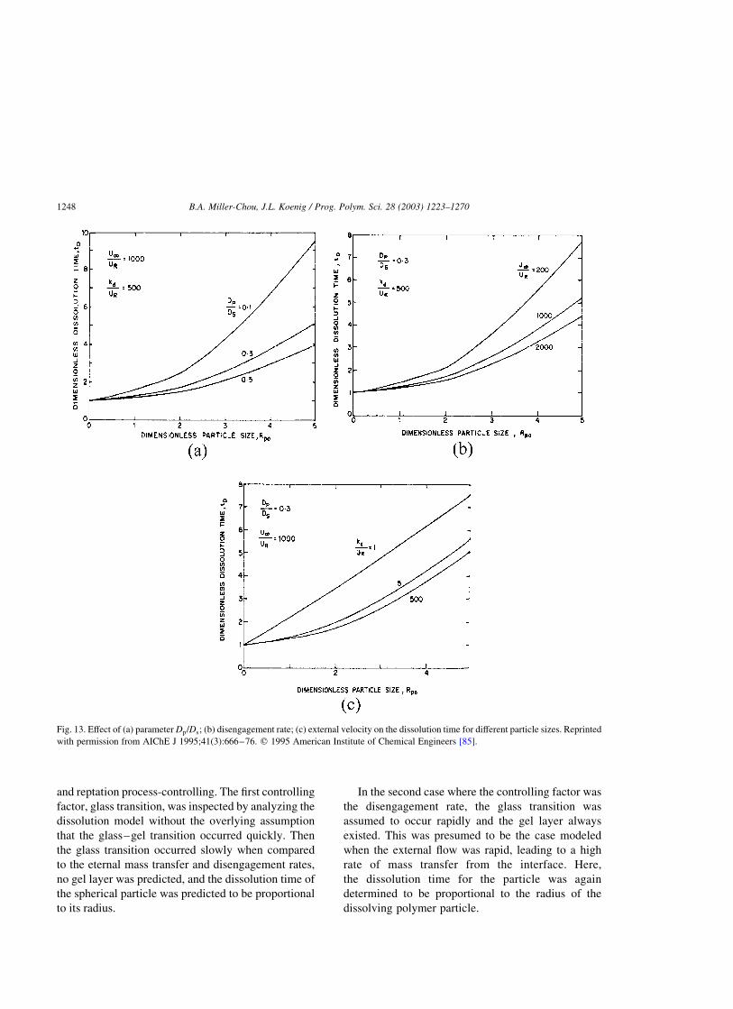
and reptation process-controlling. The first controlling

factor, glass transition, was inspected by analyzing the

dissolution model without the overlying assumption

that the glass–gel transition occurred quickly. Then

the glass transition occurred slowly when compared

to the eternal mass transfer and disengagement rates,

no gel layer was predicted, and the dissolution time of

the spherical particle was predicted to be proportional

to its radius.

In the second case where the controlling factor was

the disengagement rate, the glass transition was

assumed to occur rapidly and the gel layer always

existed. This was presumed to be the case modeled

when the external flow was rapid, leading to a high

rate of mass transfer from the interface. Here,

the dissolution time for the particle was again

determined to be proportional to the radius of the

dissolving polymer particle.

Fig. 13. Effect of (a) parameter Dp=Ds; (b) disengagement rate; (c) external velocity on the dissolution time for different particle sizes. Reprinted

with permission from AIChE J 1995;41(3):666–76. q 1995 American Institute of Chemical Engineers [85].


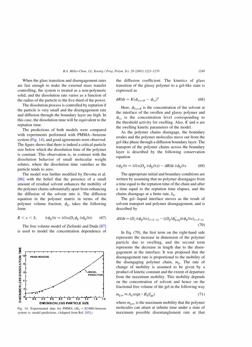
When the glass transition and disengagement rates

are fast enough to make the external mass transfer

controlling, the system is treated as a non-polymeric

solid, and the dissolution rate varies as a function of

the radius of the particle to the five-third of the power.

The dissolution process is controlled by reptation if

the particle is very small and the disengagement rate

and diffusion through the boundary layer are high. In

this case, the dissolution time will be equivalent to the

reptation time.

The predictions of both models were compared

with experiments performed with PMMA–benzene

system (Fig. 14), and good agreements were observed.

The figure shows that there is indeed a critical particle

size below which the dissolution time of the polymer

is constant. This observation is, in contrast with the

dissolution behavior of small molecular weight

solutes, where the dissolution time vanishes as the

particle tends to zero.

The model was further modified by Devotta et al.

[86] with the belief that the presence of a small

amount of residual solvent enhances the mobility of

the polymer chains substantially apart from enhancing

the diffusion of the solvent into it. The diffusion

equation in the polymer matrix in terms of the

polymer volume fraction, fp; takes the following

form

R , x , S; ›fp=›t ¼ ›=›xðDsfp ›fp=›tÞ ð67Þ

The free volume model of Zielinski and Duda [87]

is used to model the concentration dependence of

the diffusion coefficient. The kinetics of glass

transition of the glassy polymer to a gel-like state is

expressed as

dR=dt ¼ Kðfslx¼R 2 fs;tÞn ð68Þ

Here, fslx¼R is the concentration of the solvent at

the interface of the swollen and glassy polymer and

fs;t is the concentration level corresponding to

the threshold activity for swelling. Also, K and n are

the swelling kinetic parameters of the model.

As the polymer chains disengage, the boundary

erodes and the polymer molecules move out from the

gel-like phase through a diffusion boundary layer. The

transport of the polymer chains across the boundary

layer is described by the following conservation

equation

›fp=›t ¼ ›=›xðDp ›fp=›xÞ2 dR=dt ›fp=›x ð69Þ

The appropriate initial and boundary conditions are

written by assuming that no polymer disengages from

a time equal to the reptation time of the chain and after

a time equal to the reptation time elapses, and the

chains disengage at a finite rate, kd:

The gel–liquid interface moves as the result of

solvent transport and polymer disengagement, and is

described by

dS=dt ¼ ðDs ›fp=›xÞx¼S2ðtÞ2 ððDp=f2p;eqÞ›fp=›xÞx¼SþðtÞ

ð70Þ

In Eq. (70), the first term on the right-hand side

represents the increase in dimension of the polymer

particle due to swelling, and the second term

represents the decrease in length due to the disen-

gagement at the interface. It was proposed that the

disengagement rate is proportional to the mobility of

the disengaging polymer chain, mp: The rate of

change of mobility is assumed to be given by a

product of kinetic constant and the extent of departure

from the maximum mobility. This mobility depends

on the concentration of solvent and hence on the

fractional free volume of the gel in the following way

mp;//Ad expð2Bd=fgpÞ ð71Þ

where mp;/ is the maximum mobility that the polymer

molecules can attain at infinite time under a state of

maximum possible disentanglement rate at thatFig. 14. Experimental data for PMMA ðMw ¼ 82 000Þ-benzene

system vs. model predictions. (Adapted from Ref. [85].)


concentration, Bd is a parameter which depends on the

size of the mobile species, and fgp is the free volume

fraction of the gel phase and is given by

fgp ¼ fppfp þ fspð1 2 fpÞ ð72Þ

The concentration at the glassy–gel interface is

calculated by using thermodynamics of swollen

networks.

Fig. 15 shows the polymer volume fraction profiles

as a function of time, produced from simulations. The

effect of the parameter Bd on the dissolution kinetics

of the polymer is presented in Fig. 16. Bd directly

affects the surface disengagement rate. As the size of

the mobile molecule increases, the value of Bd gets

larger. For high Bd values, the dissolution rate is low

and the fraction of the chains disengaged increases

continuously with time, and it remains disengagement

limited throughout the dissolution process. However,

as the parameter Bd decreases and the disengagement

rate increases, the process is initially disengagement

limited and becomes diffusion limited when the

diffusion of the chains becomes insufficient to drive

away the disengaged chains to the bulk. Therefore, a

decrease in the dissolution rate is observed, as

observed by the plateau in Fig. 16. The effect of the

diffusion boundary layer thickness on the dissolution

mechanism is also correct and it was observed that

the mechanism shifted from disentanglement-con-

trolled to diffusion-controlled with increased thick-

nesses (Fig. 17).

4.1.3. Dissolution by mixed solvents

Devotta and Mashelkar [88] proposed a model for

polymer dissolution in mixed solvents. They assumed

that the kinetics of dissolution is completely con-

trolled by the process of disengagement of chains

from the gel–liquid interface. The diffusion of the two

solvents into the polymer film is described by

the following equations

›f1=›t ¼ ›=›xðD1 ›f1=›xÞ þ ›=›xðvsf1Þ ð73Þ

›f2=›t ¼ ›=›xðD2 ›f2=›xÞ þ ›=›xðvsf2Þ ð74Þ

where vs is the swelling velocity which is related to

the diffusion of both the solvents as follows

vs ¼ D1 ›f1=›x þ D2 ›f2=›x ð75Þ

The diffusivities of the two solvents are modeled as

dependent on their sizes and the free volume of the gel

phase, which can be expressed as

fgp ¼ fppfp þ f1pf1 þ f2pf2 ð76Þ

Fig. 15. Polymer concentration profile in the slab for slower glass

transition kinetics ðfs;t ¼ 0:15; Bd ¼ 1:5; f ps ¼ 0:3; c ¼ 0:35;

KL20=D0 ¼ 1027Þ: (Adapted from Ref. [86].)

Fig. 16. Effect of the parameter Bd on the dissolution kinetics.

d=L0 ¼ 0:15; Dp=Ds ¼ 1024; f pp ¼ 0:4; KL20=D0 ¼ 1027; fs;t ¼ 0:2:


Fig. 17. Effect of thickness of the boundary layer on the dissolution

kinetics. Bd ¼ 1:5; d=L0 ¼ 0:15; Dp=Ds ¼ 1024; f pp ¼ 0:4;

KL20=D0 ¼ 1027; fs;t ¼ 0:2: (Adapted from Ref. [86].)


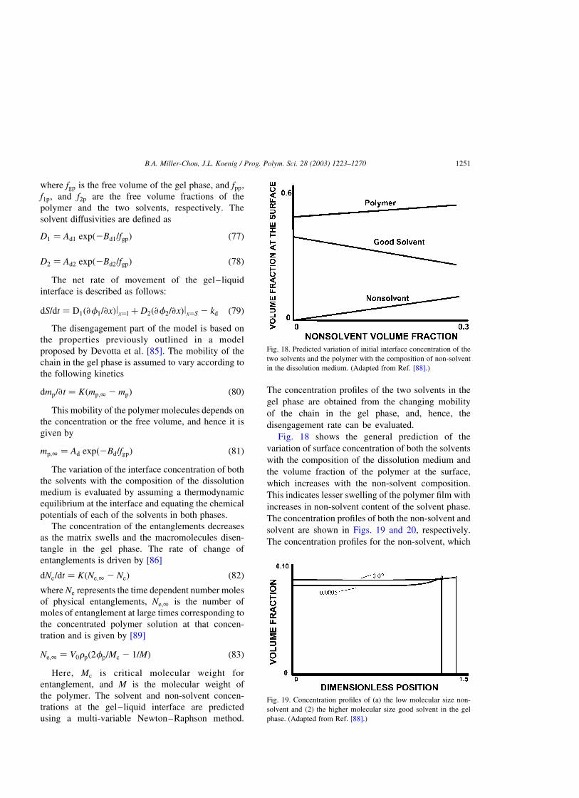
where fgp is the free volume of the gel phase, and fpp;

f1p; and f2p are the free volume fractions of the

polymer and the two solvents, respectively. The

solvent diffusivities are defined as

D1 ¼ Ad1 expð2Bd1=fgpÞ ð77Þ

D2 ¼ Ad2 expð2Bd2=fgpÞ ð78Þ

The net rate of movement of the gel–liquid

interface is described as follows:

dS=dt ¼ D1ð›f1=›xÞlx¼l þ D2ð›f2=›xÞlx¼S 2 kd ð79Þ

The disengagement part of the model is based on

the properties previously outlined in a model

proposed by Devotta et al. [85]. The mobility of the

chain in the gel phase is assumed to vary according to

the following kinetics

dmp=›t ¼ Kðmp;1 2 mpÞ ð80Þ

This mobility of the polymer molecules depends on

the concentration or the free volume, and hence it is

given by

mp;1 ¼ Ad expð2Bd=fgpÞ ð81Þ

The variation of the interface concentration of both

the solvents with the composition of the dissolution

medium is evaluated by assuming a thermodynamic

equilibrium at the interface and equating the chemical

potentials of each of the solvents in both phases.

The concentration of the entanglements decreases

as the matrix swells and the macromolecules disen-

tangle in the gel phase. The rate of change of

entanglements is driven by [86]

dNe=dt ¼ KðNe;1 2 NeÞ ð82Þ

where Ne represents the time dependent number moles

of physical entanglements, Ne;1 is the number of

moles of entanglement at large times corresponding to

the concentrated polymer solution at that concen-

tration and is given by [89]

Ne;1 ¼ V0rpð2fp=Mc 2 1=MÞ ð83Þ

Here, Mc is critical molecular weight for

entanglement, and M is the molecular weight of

the polymer. The solvent and non-solvent concen-

trations at the gel–liquid interface are predicted

using a multi-variable Newton–Raphson method.

The concentration profiles of the two solvents in the

gel phase are obtained from the changing mobility

of the chain in the gel phase, and, hence, the

disengagement rate can be evaluated.

Fig. 18 shows the general prediction of the

variation of surface concentration of both the solvents

with the composition of the dissolution medium and

the volume fraction of the polymer at the surface,

which increases with the non-solvent composition.

This indicates lesser swelling of the polymer film with

increases in non-solvent content of the solvent phase.

The concentration profiles of both the non-solvent and

solvent are shown in Figs. 19 and 20, respectively.

The concentration profiles for the non-solvent, which

Fig. 18. Predicted variation of initial interface concentration of the

two solvents and the polymer with the composition of non-solvent

in the dissolution medium. (Adapted from Ref. [88].)

Fig. 19. Concentration profiles of (a) the low molecular size non-

solvent and (2) the higher molecular size good solvent in the gel

phase. (Adapted from Ref. [88].)


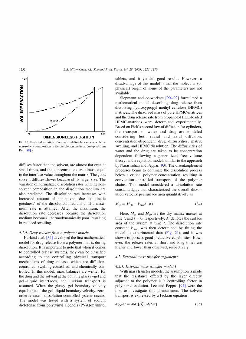
diffuses faster than the solvent, are almost flat even at

small times, and the concentrations are almost equal

to the interface value throughout the matrix. The good

solvent diffuses slower because of its larger size. The

variation of normalized dissolution rates with the non-

solvent composition in the dissolution medium are

also predicted. The dissolution rate increases with

increased amount of non-solvent due to ‘kinetic

goodness’ of the dissolution medium until a maxi-

mum rate is attained. After the maximum, the

dissolution rate decreases because the dissolution

medium becomes ‘thermodynamically poor’ resulting

in reduced swelling.

4.1.4. Drug release from a polymer matrix

Harland et al. [34] developed the first mathematical

model for drug release from a polymer matrix during

dissolution. It is important to note that when it comes

to controlled release systems, they can be classified

according to the controlling physical transport

mechanisms of drug release, which are diffusion-

controlled, swelling-controlled, and chemically con-

trolled. In this model, mass balances are written for

the drug and the solvent at the both the glassy–gel and

gel – liquid interfaces, and Fickian transport is

assumed. When the glassy–gel boundary velocity

equals that of the gel–liquid boundary velocity, zero-

order release in dissolution-controlled systems occurs.

The model was tested with a system of sodium

diclofenac from poly(vinyl alcohol) (PVA)-mannitol

tablets, and it yielded good results. However, a

disadvantage of this model is that the molecular (or

physical) origin of some of the parameters are not

available.

Siepmann and co-workers [90–92] formulated a

mathematical model describing drug release from

dissolving hydroxypropyl methyl cellulose (HPMC)

matrices. The dissolved mass of pure HPMC-matrices

and the drug release rate from propanolol HCL-loaded

HPMC-matrices were determined experimentally.

Based on Fick’s second law of diffusion for cylinders,

the transport of water and drug are modeled

considering both radial and axial diffusion,

concentration-dependent drug diffusivities, matrix

swelling, and HPMC dissolution. The diffusivities of

water and the drug are taken to be concentration

dependent following a generalized free volume

theory, and a reptation model, similar to the approach

by Narasimhan and Peppas [93]. The disentanglement

processes begin to dominate the dissolution process

below a critical polymer concentration, resulting in

convection-controlled transport of the polymer

chains. This model considered a dissolution rate

constant, kdiss; that characterized the overall dissol-

ution velocity per surface area quantitatively as

Mpt ¼ Mp0 2 kdissAt £ t ð84Þ

Here, Mpt and Mp0 are the dry matrix masses at

time t; and t ¼ 0; respectively, At denotes the surface

area of the system at time t: The dissolution rate

constant kdiss; was then determined by fitting the

model to experimental data (Fig. 21), and it was

shown to possess good predictive capabilities. How-

ever, the release rates at short and long times are

higher and lower than observed, respectively.

4.2. External mass transfer arguments

4.2.1. External mass transfer model I

With mass transfer models, the assumption is made

that the resistance offered by the layer directly

adjacent to the polymer is a controlling factor in

polymer dissolution. Lee and Peppas [94] were the

first to investigate this phenomenon. The solvent

transport is expressed by a Fickian equation

›fs=›t ¼ ›=›x½Dvs ›fs=›x� ð85Þ

Fig. 20. Predicted variation of normalized dissolution rates with the

non-solvent composition in the dissolution medium. (Adapted from

Ref. [88].)


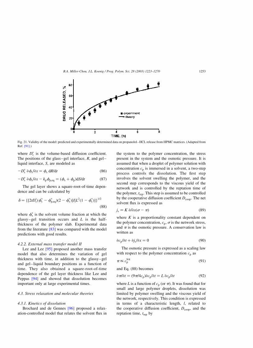
where Dvs is the volume-based diffusion coefficient.

The positions of the glass–gel interface, R; and gel–

liquid interface, S; are modeled as

2Dvs ›fs=›x ¼ fs dR=dt ð86Þ

2Dvs ›fs=›x 2 kpfp;eq ¼ ðfs þ fpÞdS=dt ð87Þ

The gel layer shows a square-root-of-time depen-

dence and can be calculated by

d ¼ {½2tDvs ðf

ps 2 fp

p;eqÞð2 2 fps Þ�=½L

2ð1 2 fps Þ�}

1=2

ð88Þ

where fps is the solvent volume fraction at which the

glassy–gel transition occurs and L is the half-

thickness of the polymer slab. Experimental data

from the literature [83] was compared with the model

predictions with good results.

4.2.2. External mass transfer model II

Lee and Lee [95] proposed another mass transfer

model that also determines the variation of gel

thickness with time, in addition to the glassy–gel

and gel–liquid boundary positions as a function of

time. They also obtained a square-root-of-time

dependence of the gel layer thickness like Lee and

Peppas [94] and showed that dissolution becomes

important only at large experimental times.

4.3. Stress relaxation and molecular theories

4.3.1. Kinetics of dissolution

Brochard and de Gennes [96] proposed a relax-

ation-controlled model that relates the solvent flux in

the system to the polymer concentration, the stress

present in the system and the osmotic pressure. It is

assumed that when a droplet of polymer solution with

concentration cp is immersed in a solvent, a two-step

process controls the dissolution. The first step

involves the solvent swelling the polymer, and the

second step corresponds to the viscous yield of the

network and is controlled by the reptation time of

the polymer, trep: This step is assumed to be controlled

by the cooperative diffusion coefficient Dcoop: The net

solvent flux is expressed as

js ¼ K ›=›xðs2 pÞ ð89Þ

where K is a proportionality constant dependent on

the polymer concentration, cp; s is the network stress,

and p is the osmotic pressure. A conservation law is

written as

›cp=›t þ ›js=›x ¼ 0 ð90Þ

The osmotic pressure is expressed as a scaling law

with respect to the polymer concentration cp as

p/ c9=4p ð91Þ

and Eq. (88) becomes

›p=›t ¼ ð9p=4cpÞ›cp=›t ¼ L ›cp=›t ð92Þ

where L is a function of cp (or p). It was found that for

small and large polymer droplets, dissolution was

limited by polymer swelling and the viscous yield of

the network, respectively. This condition is expressed

in terms of a characteristic length, l; related to

the cooperative diffusion coefficient, Dcoop; and the

reptation time, trep by

Fig. 21. Validity of the model: predicted and experimentally determined data on propanolol–HCL release from HPMC matrices. (Adapted from

Ref. [91].)


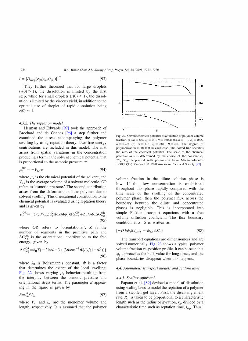
l ¼ ½Dcoopðcp0Þtrepðcp0Þ�1=2 ð93Þ

They further theorized that for large droplets

ðrð0Þ . 1Þ; the dissolution is limited by the first

step, while for small droplets ðrð0Þ , 1Þ; the dissol-

ution is limited by the viscous yield, in addition to the

optimal size of droplet of rapid dissolution being

rð0Þ , 1:

4.3.2. The reptation model

Herman and Edwards [97] took the approach of

Brochard and de Gennes [96] a step further and

examined the stress accompanying the polymer

swelling by using reptation theory. Two free energy

contributions are included in this model. The first

arises from spatial variations in the concentration

producing a term in the solvent chemical potential that

is proportional to the osmotic pressure p

mOPs ¼ 2Va;sp ð94Þ

where ms is the chemical potential of the solvent, and

Va;s is the average volume of a solvent molecule. OP

refers to ‘osmotic pressure.’ The second contribution

arises from the deformation of the polymer due to

solvent swelling. This orientational contribution to the

chemical potential is evaluated using reptation theory

and is given by

mORs ¼2ðVa;s=Va;pÞf

2p½ðdZ=dfpÞDGOR

segþZ›=›fpDGORseg�

ð95Þ

where OR refers to ‘orientational’, Z is the

number of segments in the primitive path and

DGORseg is the orientational contribution to the free

energy, given by

DGORseg¼kBT{22lnF23þ½3Fcos21F�=½

pð12F2Þ�}

ð96Þ

where kB is Boltzmann’s constant, F is a factor

that determines the extent of the local swelling.

Fig. 22 shows varying ms behavior resulting from

the interplay between the osmotic pressure and

orientational stress terms. The parameter B appear-

ing in the figure is given by

B¼l3m=Vm ð97Þ

where Vm and lm are the monomer volume and

length, respectively. It is assumed that the polymer

volume fraction in the dilute solution phase is

low. If this low concentration is established

throughout this phase rapidly compared with the

time scale of the swelling of the concentrated

polymer phase, then the polymer flux across the

boundary between the dilute and concentrated

phases is negligible. This is incorporated into

simple Fickian transport equations with a free

volume diffusion coefficient. The flux boundary

condition at x¼S is written as

½2D ›fp›x�x¼S ¼ fp;b dS=dt ð98Þ

The transport equations are dimensionless and are

solved numerically. Fig. 23 shows a typical polymer

volume fraction vs. position profile. It can be seen that

fp approaches the bulk value for long times, and the

phase boundaries disappear when this happens.

4.4. Anomalous transport models and scaling laws

4.4.1. Scaling approach

Papanu et al. [89] devised a model of dissolution

using scaling laws to model the reptation of a polymer

from a swollen gel layer. First, the disentanglement

rate, Rd; is taken to be proportional to a characteristic

length such as the radius or gyration, rg; divided by a

characteristic time such as reptation time, trep: Thus,

Fig. 22. Solvent chemical potential as a function of polymer volume

fraction. (a) m ¼ 8:0; Zs ¼ 0:1; B ¼ 0:064; (b) m ¼ 1:0; Zs ¼ 0:05;

B ¼ 0:26; (c) m ¼ 1:0; Zs ¼ 0:01; B ¼ 2:6: The degree of

polymerization is 10 000 in each case. The dotted line specifies

the zero of the chemical potential. The scale of the chemical

potential axis is determined by the choice of the constant kB

TVa;s=Va;p: Reprinted with permission from Macromolecules

1990;23(15):3662–71. q 1990 American Chemical Society [97].


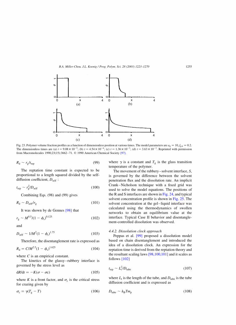
Rd , rg=trep ð99Þ

The reptation time constant is expected to be

proportional to a length squared divided by the self-

diffusion coefficient, Dself :

trep , r2g=Dself ð100Þ

Combining Eqs. (98) and (99) gives

Rd , Dself =rg ð101Þ

It was shown by de Gennes [98] that

rg , M0:5=ð1 2 fsÞ

0:125 ð102Þ

and

Dself , 1=M2ð1 2 fsÞ1:75 ð103Þ

Therefore, the disentanglement rate is expressed as

Rd ¼ C=M2:5ð1 2 fsÞ1:625 ð104Þ

where C is an empirical constant.

The kinetics of the glassy–rubbery interface is

governed by the stress level as

dR=dt ¼ 2Kðs2 scÞ ð105Þ

where K is a front factor, and sc is the critical stress

for crazing given by

sc ¼ gðTg 2 TÞ ð106Þ

where g is a constant and Tg is the glass transition

temperature of the polymer.

The movement of the rubbery–solvent interface, S;

is governed by the difference between the solvent

penetration flux and the dissolution rate. An implicit

Crank–Nicholson technique with a fixed grid was

used to solve the model equations. The positions of

the R and S interfaces are shown in Fig. 24, and typical

solvent concentration profile is shown in Fig. 25. The

solvent concentration at the gel–liquid interface was

calculated using the thermodynamics of swollen

networks to obtain an equilibrium value at the

interface. Typical Case II behavior and disentangle-

ment-controlled dissolution was observed.

4.4.2. Dissolution clock approach

Peppas et al. [99] proposed a dissolution model

based on chain disentanglement and introduced the

idea of a dissolution clock. An expression for the

reptation time is derived from the reptation theory and

the resultant scaling laws [98,100,101] and it scales as

follows [102]

trep , L2t =Dtube ð107Þ

where Lt is the length of the tube, and Dtube is the tube

diffusion coefficient and is expressed as

Dtube , kBTmp ð108Þ

Fig. 23. Polymer volume fraction profiles as a function of dimensionless position at various times. The model parameters are ad ¼ 10; fp;b ¼ 0:2:

The dimensionless times are (a) t ¼ 9:08 £ 1025; (b) t ¼ 4:54 £ 1024; (c) t ¼ 1:36 £ 1023; (d) t ¼ 3:63 £ 1023: Reprinted with permission

from Macromolecules 1990;23(15):3662–71. q 1990 American Chemical Society [97].


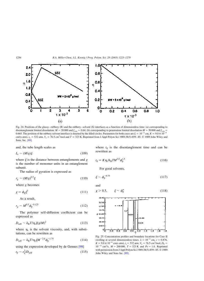
and, the tube length scales as

Lt , ðM=gÞj ð109Þ

where j is the distance between entanglements and g

is the number of monomer units in an entanglement

subunit.

The radius of gyration is expressed as

rg , ðM=gÞ0:5j ð110Þ

where g becomes

g ¼ fpj3 ð111Þ

As a result,

rg , M0:5f20:125p ð112Þ

The polymer self-diffusion coefficient can be

expressed as

Dself , kBT =hsjðg=MÞ2 ð113Þ

where hs is the solvent viscosity, and, with substi-

tutions, can be rewritten as

Dself , kBT =hsjM22:0f21:75p ð114Þ

using the expression developed by de Gennes [98]

td , r2g=Dself ð115Þ

where td is the disentanglement time and can be

rewritten as

td ¼ Khs=kBTM3:0f1:5p ð116Þ

For good solvents,

j , f20:75p ð117Þ

and

x . 0:5; j , fap ð118Þ

Fig. 24. Positions of the glassy–rubbery (R) and the rubbery–solvent (S) interfaces as a function of dimensionless time: (a) corresponding to

disentanglement limited dissolution: M ¼ 20 000 and fs;eq ¼ 0:64; (b) corresponding to penetration limited dissolution-M ¼ 50 000 and fs;eq ¼

0:665: The position of the rubbery solvent interface is denoted by the filled circles. Parameters for both cases are L ¼ 1024 cm; K ¼ 9:0 £ 1029

cm=ðs atmÞ; sc ¼ 532 atm; Vs ¼ 76:5 cm3=mol and T ¼ 323 K: Reprinted from J Appl Polym Sci 1989;38(5):859–85. q 1989 John Wiley and

Sons, Inc. [89].

Fig. 25. Concentration profiles and boundary locations for Case II

swelling at several dimensionless times. L ¼ 1024 cm; c ¼ 0:876;

K ¼ 9:0 £ 1029 cmðs atmÞ; ðc¼ 532 atm; Vs ¼ 76:5 cm3=mol; D0 ¼

10211 cm2=s; M ¼ 200 000; T ¼ 323 K and Pe ¼ 1:0: Reprinted

with permission from J Appl Polym Sci 1989;38(5):859–85.q 1989

John Wiley and Sons Inc. [89].


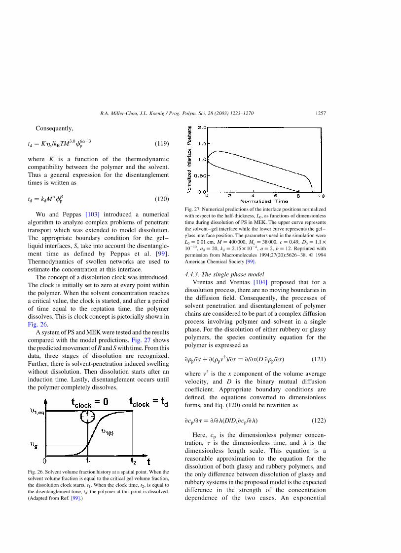
Consequently,

td ¼ Khs=kBTM3:0f6a23p ð119Þ

where K is a function of the thermodynamic

compatibility between the polymer and the solvent.

Thus a general expression for the disentanglement

times is written as

td ¼ kdMafbp ð120Þ

Wu and Peppas [103] introduced a numerical

algorithm to analyze complex problems of penetrant

transport which was extended to model dissolution.

The appropriate boundary condition for the gel–

liquid interfaces, S; take into account the disentangle-

ment time as defined by Peppas et al. [99].

Thermodynamics of swollen networks are used to

estimate the concentration at this interface.

The concept of a dissolution clock was introduced.

The clock is initially set to zero at every point within

the polymer. When the solvent concentration reaches

a critical value, the clock is started, and after a period

of time equal to the reptation time, the polymer

dissolves. This is clock concept is pictorially shown in

Fig. 26.

A system of PS and MEK were tested and the results

compared with the model predictions. Fig. 27 shows

the predicted movement of R and S with time. From this

data, three stages of dissolution are recognized.

Further, there is solvent-penetration induced swelling

without dissolution. Then dissolution starts after an

induction time. Lastly, disentanglement occurs until

the polymer completely dissolves.

4.4.3. The single phase model

Vrentas and Vrentas [104] proposed that for a

dissolution process, there are no moving boundaries in

the diffusion field. Consequently, the processes of

solvent penetration and disentanglement of polymer

chains are considered to be part of a complex diffusion

process involving polymer and solvent in a single

phase. For the dissolution of either rubbery or glassy

polymers, the species continuity equation for the

polymer is expressed as

›rp=›t þ ›ðrpv†Þ=›x ¼ ›=›xðD ›rp=›xÞ ð121Þ

where v† is the x component of the volume average

velocity, and D is the binary mutual diffusion

coefficient. Appropriate boundary conditions are

defined, the equations converted to dimensionless

forms, and Eq. (120) could be rewritten as

›cp=›t ¼ ›=›lðD=Ds›cp=›lÞ ð122Þ

Here, cp is the dimensionless polymer concen-

tration, t is the dimensionless time, and l is the

dimensionless length scale. This equation is a

reasonable approximation to the equation for the

dissolution of both glassy and rubbery polymers, and

the only difference between dissolution of glassy and

rubbery systems in the proposed model is the expected

difference in the strength of the concentration

dependence of the two cases. An exponential

Fig. 26. Solvent volume fraction history at a spatial point. When the

solvent volume fraction is equal to the critical gel volume fraction,

the dissolution clock starts, t1: When the clock time, t2; is equal to

the disentanglement time, td; the polymer at this point is dissolved.


Fig. 27. Numerical predictions of the interface positions normalized

with respect to the half-thickness, L0; as functions of dimensionless

time during dissolution of PS in MEK. The upper curve represents

the solvent–gel interface while the lower curve represents the gel–

glass interface position. The parameters used in the simulation were

L0 ¼ 0:01 cm; M ¼ 400 000; Mc ¼ 38 000; c ¼ 0:49; D0 ¼ 1:1 £

10210; ad ¼ 20; kd ¼ 2:15 £ 1024; a ¼ 2; b ¼ 12: Reprinted with

permission from Macromolecules 1994;27(20):5626–38. q 1994

American Chemical Society [99].


concentration dependence of the mutual diffusion

coefficient is expressed as follows

kcp $ 0; D=Ds ¼ expð2kcpÞ ð123Þ

Therefore, the strength of the concentration

dependence can be characterized by a ratio, r; as

follows

r ¼ Dðcp ¼ 0Þ=DðC ¼ 1Þ ¼ expðkÞ ð124Þ

The concentration distribution in the liquid phase

can thus be determined for the dissolution of the

polymer. Dissolution curves are constructed by

plotting the fraction of polymer which dissolves

versus the square root of dimensionless time (Fig. 28).

The dissolution curves are linear in the early stages of

dissolution. For r ¼ 1 and 10, the slopes of the curves

decrease with increasing times, but for sufficiently

high values of r; it becomes evident that there is an

increase in the slopes before the dissolution curves

eventfully flatten to the value of unity. As a result, it

appears that the dissolution curves assume sigmoidal

shapes for sufficiently high values of r: It was

concluded that the dissolution process was

only moderately sensitive to the strength of

the concentration dependence of the mutual diffusion

coefficient. The dimensionless time when the fraction

dissolves is equal to 1/2, the half-time for dissolution.

Even though it is assumed that the dissolution

process involves only one phase with no interfaces, it

is possible to suppose that pseudointerfaces exist at

certain dimensionless polymer concentrations.

4.5. Molecular theories in a continuum framework

4.5.1. Dissolution of a rubbery polymer

Narasimhan and Peppas [105] analyzed the

dissolution mechanism of rubbery polymers by

dividing the penetrant concentration field into

three regimes that delineated three distinctly

different transport processes (Fig. 29). The first

regime consists of the swollen rubber and is

deemed the ‘concentrated’ regime. The existence

of a diffusion boundary layer adjacent to the

rubber–liquid interface, S; is defined as the ‘semi-

dilute’ regime. The ‘dilute’ regime is defined when

the polymer is fully dissolved and the disentangled

chains move freely in the solvent, exhibiting

Brownian motion.

Because the solvent transport through rubbery

polymers is generally known to be Fickian, the

solvent penetration is presented as

›fs=›t ¼ ›=›xðD ›fs=›xÞ ð125Þ

Appropriate boundary conditions are defined.

As the macromolecules disentangle, they move out

of the gel-like phase to a liquid solution through a

diffusion boundary layer of thickness, d; which is

assumed to be constant. The chain transport through

this boundary layer is described as

›fp=›t ¼ ›=›xðDp ›fp=›xÞ2 dS=dt ›fp=›x ð126Þ

This equation is valid in the region between x ¼ S

and x ¼ S þ d; and the initial boundary conditions

are

t ¼ 0; fp ¼ 0 ð127Þ

Fig. 29. Disentanglement of polymer chains (a) before dissolution

starts, there is no disentanglement; this is a swellable system. (b)

This depicts the onset of dissolution in the diffusion boundary layer.

(c) The dissolution is complete and the disentangled chains exhibit

Brownian motion in the solvent. (Adapted from Ref. [104].)

Fig. 28. Dissolution curves for four values of r; the diffusivity ratio

defined by Eq. (124). (Adapted from Ref. [104].)


At the end of the boundary layer, the conventional

boundary condition is

x 2 SðtÞ þ d; fp ¼ 0 ð128Þ

The boundary condition on the solvent side of the

rubber–liquid interface is written by considering that

a polymer chain requires a minimum time to

disentangle and move out of the gel. This minimum

time is the reptation time, trep: Hence, the disen-

tanglement rate is zero until a time equal to the

reptation time elapses:

2Dp ›fp=›x ¼ 0; x ¼ SþðtÞ;

0 , t , trep 2 Dp ›fp=›x ¼ 0

ð129Þ

After the reptation time is complete, the transport

of the chains at the rubber–liquid interface may be

disentanglement-limited or diffusion-limited. The rate

of diffusion is sufficiently high at times just greater

than trep; so the flux is disentanglement-limited.

Therefore, the boundary condition was written as

2Dp ›fp=›x ¼ kd; x ¼ SþðtÞ; t , trep ð130Þ

The polymer concentration in the boundary layer

eventually reaches an equilibrium value, fp;eq; and the

diffusion rate becomes insufficient to transport the

chains, at which point this polymer concentration is

maintained. It was proposed that an equilibrium exists

between the polymer-rich gel and the polymer-lean

solvent in the diffusion boundary layer, and the

boundary condition becomes

x ¼ SþðtÞ; fþp ¼ fp;eq; t , trep ð131Þ

As the solvent swells the polymer, the rubber–

liquid interface S moves and this is expressed as

dS=dt ¼ ðD ›fp=›xÞ2 2 Dp=f2s ð›fp=›xÞþ; Sð0Þ ¼ 1

ð132Þ

It is shown that there exists a critical solvent

concentration fs;c; at which the diffusivity of the

system changes as follows

D ¼ Ds; fs , fs;c ð133Þ

D ¼ Dp; fs . fs;c ð134Þ

where

Ds ¼ Ds;0 expðadfsÞ ð135Þ

and Ds;0 is the diffusivity of the solvent in a glassy

polymer and Dp is a ‘reptation’ diffusion coefficient.

It is postulated that for a dissolving polymer, the

disentanglement rate, kd; is the ratio of the radius of

gyration rg; to the reptation time, trep :

kd ¼ rg=trep ð136Þ

This assumption is made based on previous work

[98,102] showing that a polymer requires a time

equivalent to its reptation time to disentangle and that

the distance that the chain travels during that time can

be approximated by its radius of gyration.

The model was tested and typical profiles for the

solvent volume fraction as a function of position and

time in the rubber and the polymer volume fraction in

the diffusion boundary layer are shown in Figs. 30

and 31. Other features of the simulation are the

prediction of the temporal evolution of the rubber–

solvent interface and the mass fraction of the polymer

dissolved as a function of time (Figs. 32 and 33). The

simulations showed that the dissolution is either

disentanglement- or diffusion-controlled depending

on the polymer molecular weight and the thickness of

the diffusion boundary layer.

4.5.2. Dissolution of a glassy polymer

Narasimhan and Peppas [106] extended their

previous dissolution model for rubbery polymers

Fig. 30. Solvent volume fraction, fs as a function of position, x: The

polymer molecular weight was M ¼ 40 000 and trep ¼ 1000 s: The

position x ¼ 0 is the center of the slab. The time increment starting

from the first curve on the right is Dt ¼ 1000 s: (Adapted from Ref.

[105].)


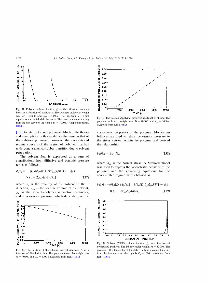
[105] to interpret glassy polymers. Much of the theory

and assumptions in this model are the same as that of

the rubbery polymers, however, the concentrated

regime consists of the region of polymer that has

undergone a glass-to-rubber transition due to solvent

penetration.

The solvent flux is expressed as a sum of

contributions from diffusive and osmotic pressure

terms as follows:

fsvs ¼2 ½D ›fs=›x þ DVs;sfs=RTð1 2 fsÞ

ð1 2 2xspfsÞ›p=›x� ð137Þ

where vs is the velocity of the solvent in the x

direction, Vs;s is the specific volume of the solvent,

xsp is the solvent–polymer interaction parameter,

and p is osmotic pressure, which depends upon the

viscoelastic properties of the polymer. Momentum

balances are used to relate the osmotic pressure to

the stress existent within the polymer and derived

the relationship

›p=›x ¼ ›sxx=›x ð138Þ

where sxx is the normal stress. A Maxwell model

was used to express the viscoelastic behavior of the

polymer and the governing equations for the

concentrated regime were obtained as

›fs=›t ¼›=›x½D ›fs=›x� þ ›=›x½DVs;sfs=RTð1 2 fsÞ

ð1 2 2xspfsÞ›s=›x� ð139Þ

Fig. 31. Polymer volume fraction, fs; in the diffusion boundary

layer, as a function of position, s: The polymer molecular weight

was M ¼ 40 000 and trep ¼ 1000 s: The position x ¼ 5 mm

represents the initial slab thickness. The time increment starting

from the first curve on the right is Dt ¼ 1000 s: (Adapted from Ref.

[105].)

Fig. 33. The fraction of polymer dissolved as a function of time. The

polymer molecular weight was M ¼ 40 000 and trep ¼ 1000 s:


Fig. 32. The position of the rubbery–solvent interface, S; as a

function of dissolution time The polymer molecular weight was

M ¼ 40 000 and trep ¼ 1000 s: (Adapted from Ref. [105].)

Fig. 34. Solvent (MEK) volume fraction, fs; as a function of

normalized position. The PS molecular weight M ¼ 52 000: The

position ¼ 0 is the center of the slab. The time increment starting

from the first curve on the right is Dt ¼ 1000 s: (Adapted from

Ref. [106].)


›sxx=›t ¼ 2sxx=ðh=EÞ þ E=ð1 2 fsÞ2›fs=›t ð140Þ

where h is viscosity, and E is the spring modulus.

A mathematical simulation of the model was tested

using a system consisting of PS dissolving in MEK.

Fig. 34 shows the solvent volume fraction in the

polymer as a function of time and position. The

position of the interfaces R and S as a function of time

are shown in Fig. 35. Integrating the concentration

profiles, the mass fraction of polymer dissolved as a

function of time was obtained (Fig. 36). Upon

increasing the polymer molecular weight, the dissol-

ution became disentanglement-controlled, but

decreasing the diffusion boundary layer thickness

shifted the dissolution mechanism to diffusion-

controlled.

4.5.3. Molecular model for drug release I

Narasimhan and Peppas modified the phenomen-

ological drug delivery model developed by Harland

et al. [34] by applying their models [105,106] and

incorporating the macromolecular chain disentangle-

ment. A three-component system is considered, with

water as component 1, the polymer as component 2,

and the drug component 3. The model considers the

two moving boundaries, R and S; previously discussed

in their models for rubbery and glassy polymer

dissolutions. Quasiequilibrium conditions at the

rubbery–solvent interface enable the use of the

Flory–Rehneer theory [106] to calculate the water

and drug volume fractions at this interface. The

variation of the gel layer thickness ðS–RÞ with time is

obtained as

2ðS–RÞ=BC 2 ðAC=B2CÞln½1 2 ðBC=ACÞðS–RÞ� ¼ t

ð141Þ

where

AC ¼ DSðfs;eq 2 fscÞ½fs;eq=fs;eq þ fd;eq

þ 1=ðfsc þ fdcÞ� þ Ddðfdc 2 fd;eqÞ

½fd;eq=ðfs;eq þ fd;eqÞ þ 1=ðfsc þ fdcÞ� ð142Þ

BC ¼ kd=ðfs;eq þ fd;eqÞ ð143Þ

and an expression for the fraction of the drug released

is derived as

Md=Md;1 ¼ ðfd;eq þ fdcÞ=2lðð2ACtÞ1=2 þ BCt ð144Þ

where l is the half-thickness of the polymer, fsc and

fdc are characteristic concentrations of solvent and

drug, respectively, fs;eq and fd;eq are equilibrium

concentrations of solvent and drug, respectively, kd

is the disentanglement rate of the polymer chains.

Fig. 37 shows the predicted normalized gel layer

thickness as a function of normalized time for

different values of AC=BC: As AC=BC approaches

zero, the gel layer thickness profile becomes flat

(disentanglement-controlled) while for higher values

of AC=BC; then it increases with time (diffusion-

controlled). Model predictions were compared with

experimental results [93,107] and were in good

agreement.Fig. 36. Fraction of PS dissolved as a function of time. The PS

molecular weight M ¼ 52 000: (Adapted from Ref. [106].)

Fig. 35. Rubbery–solvent interface (S), glassy–rubbery interface

(R), and gel layer thickness (S–R) as a function of normalized

position. The PS molecular weight M ¼ 52 000: (Adapted from

Ref. [106].)


4.5.4. Molecular model for drug release II

Ju et al. [108–110] proposed a mathematical

model of drug release from hydrophilic matrices

based on the diffusion layer and a polymer disen-

tanglement concentration, rp;dis; which is defined as

the concentration below which the chains detach

from the matrix and diffuse through the diffusion layer

into the bulk solution and scaled as

rp;dis , M20:8 ð145Þ

The mathematical description of the transport

accounts for swelling/dissolution in the radial direc-

tion and also derives ‘universal’ scaling relationships

for the fraction release of both polymer and drug with

respect to the polymer molecular weight, M: A weaker

molecular weight dependence for the drug is pre-

dicted, and, for very large values of M; both fractional

release profiles approach limiting values. These

results agree well with experimental data on fractional

release of HPMC and adinazolam mesylate form

HPMC matrices of various molecular weights.

Ju et al. also developed a model for the diffusion

coefficients of disentangled HPMC chains in the

diffusion layer adjacent to the matrix [110]. They

showed that the effective diffusion coefficient scales

with M as

Deff , M20:53 ð146Þ

and the chains exhibit Zimm dynamics [111] within

the diffusion layer regime, providing a scaling

relationship of

DZimm , M20:5 ð147Þ

which is very close to the result that they derived.

5. Techniques used to study polymer dissolution

Various experimental techniques have been uti-

lized to characterize polymer dissolution behavior.

Some of these techniques include differential refrac-

tometry, optical microscopy, fluorescence, gravime-

try, interferometry, NMR, and FT-IR imaging. This

section describes these techniques and how they are

used to monitor polymer dissolution. The advantages

and disadvantages of the methods are also be

discussed.

5.1. Differential refractometry

One of the earliest techniques used to study

polymer dissolution was refractometry [12]. The

basis of this technique is that during the dissolution

process, the polymer concentration increases continu-

ously in the solvent, and this concentration can be

measured by the refractive index. While this tech-

nique provides some measurements of the dissolution

process and detects small changes in polymer

concentration in the solvent phase, no information

can be obtained about the surface layer of the polymer

pellet. Also, when a relatively small amount of

polymer is being dissolved in very large quantities

of solvent, this method is less satisfactory than when

larger quantities of polymer are being dissolved.

5.2. Optical microscopy

Optical microscopy allows direct visual obser-

vation of the dissolution process and the formation of

a gel layer. Therefore, it provides information about

the structures of the different layers (solvent, gel, and

polymer layers) formed, which can govern the

dissolution process. The apparatus used consists of a

microscope and a sample cell composed of a slice of

polymer pellet encapsulated in a matrix inert to the

solvent, which is then sandwiched between two glass

slides (Fig. 38). In cases where both the solvent and

Fig. 37. Predicted normalized gel layer thickness, d=l as a function

of normalized time, t; for different values of AC=BC: (Adapted from

Ref. [93].)


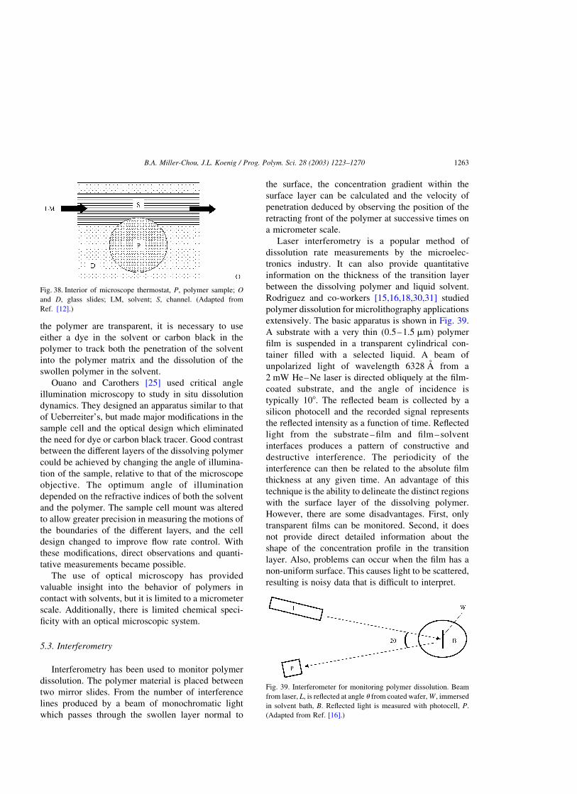
the polymer are transparent, it is necessary to use

either a dye in the solvent or carbon black in the

polymer to track both the penetration of the solvent

into the polymer matrix and the dissolution of the

swollen polymer in the solvent.

Ouano and Carothers [25] used critical angle

illumination microscopy to study in situ dissolution

dynamics. They designed an apparatus similar to that

of Ueberreiter’s, but made major modifications in the

sample cell and the optical design which eliminated

the need for dye or carbon black tracer. Good contrast

between the different layers of the dissolving polymer

could be achieved by changing the angle of illumina-

tion of the sample, relative to that of the microscope

objective. The optimum angle of illumination

depended on the refractive indices of both the solvent

and the polymer. The sample cell mount was altered

to allow greater precision in measuring the motions of

the boundaries of the different layers, and the cell

design changed to improve flow rate control. With

these modifications, direct observations and quanti-

tative measurements became possible.

The use of optical microscopy has provided

valuable insight into the behavior of polymers in

contact with solvents, but it is limited to a micrometer

scale. Additionally, there is limited chemical speci-

ficity with an optical microscopic system.

5.3. Interferometry

Interferometry has been used to monitor polymer

dissolution. The polymer material is placed between

two mirror slides. From the number of interference

lines produced by a beam of monochromatic light

which passes through the swollen layer normal to

the surface, the concentration gradient within the

surface layer can be calculated and the velocity of

penetration deduced by observing the position of the

retracting front of the polymer at successive times on

a micrometer scale.

Laser interferometry is a popular method of

dissolution rate measurements by the microelec-

tronics industry. It can also provide quantitative

information on the thickness of the transition layer

between the dissolving polymer and liquid solvent.

Rodriguez and co-workers [15,16,18,30,31] studied

polymer dissolution for microlithography applications

extensively. The basic apparatus is shown in Fig. 39.

A substrate with a very thin (0.5–1.5 mm) polymer

film is suspended in a transparent cylindrical con-

tainer filled with a selected liquid. A beam of

unpolarized light of wavelength 6328 A from a

2 mW He–Ne laser is directed obliquely at the film-

coated substrate, and the angle of incidence is

typically 108. The reflected beam is collected by a

silicon photocell and the recorded signal represents

the reflected intensity as a function of time. Reflected

light from the substrate–film and film–solvent

interfaces produces a pattern of constructive and

destructive interference. The periodicity of the

interference can then be related to the absolute film

thickness at any given time. An advantage of this

technique is the ability to delineate the distinct regions

with the surface layer of the dissolving polymer.

However, there are some disadvantages. First, only

transparent films can be monitored. Second, it does

not provide direct detailed information about the

shape of the concentration profile in the transition

layer. Also, problems can occur when the film has a

non-uniform surface. This causes light to be scattered,

resulting is noisy data that is difficult to interpret.

Fig. 38. Interior of microscope thermostat, P; polymer sample; O

and D; glass slides; LM, solvent; S, channel. (Adapted from

Ref. [12].)

Fig. 39. Interferometer for monitoring polymer dissolution. Beam

from laser, L; is reflected at angle u from coated wafer, W ; immersed

in solvent bath, B: Reflected light is measured with photocell, P:



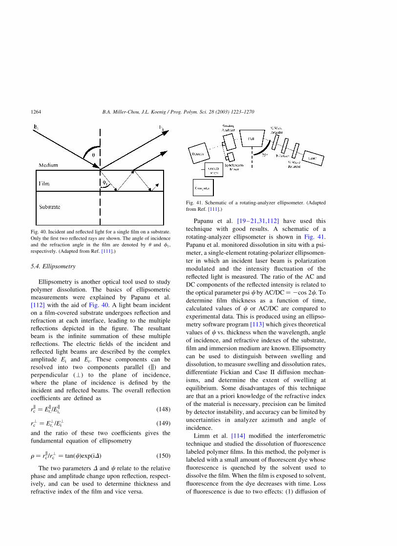
5.4. Ellipsometry

Ellipsometry is another optical tool used to study

polymer dissolution. The basics of ellipsometric

measurements were explained by Papanu et al.

[112] with the aid of Fig. 40. A light beam incident

on a film-covered substrate undergoes reflection and

refraction at each interface, leading to the multiple

reflections depicted in the figure. The resultant

beam is the infinite summation of these multiple

reflections. The electric fields of the incident and

reflected light beams are described by the complex

amplitude Ei and Er: These components can be

resolved into two components parallel (k) and

perpendicular (’) to the plane of incidence,

where the plane of incidence is defined by the

incident and reflected beams. The overall reflection

coefficients are defined as

rkc ¼ Ekr;=E

ki; ð148Þ

r’c ¼ E’r; =E

’i ð149Þ

and the ratio of these two coefficients gives the

fundamental equation of ellipsometry

r ¼ rkc =r’c ¼ tanðcÞexpðiDÞ ð150Þ

The two parameters D and c relate to the relative

phase and amplitude change upon reflection, respect-

ively, and can be used to determine thickness and

refractive index of the film and vice versa.

Papanu et al. [19–21,31,112] have used this

technique with good results. A schematic of a

rotating-analyzer ellipsometer is shown in Fig. 41.

Papanu et al. monitored dissolution in situ with a psi-

meter, a single-element rotating-polarizer ellipsomen-

ter in which an incident laser beam is polarization

modulated and the intensity fluctuation of the

reflected light is measured. The ratio of the AC and

DC components of the reflected intensity is related to

the optical parameter psi c by AC/DC ¼ 2cos 2c: To

determine film thickness as a function of time,

calculated values of c or AC/DC are compared to

experimental data. This is produced using an ellipso-

metry software program [113] which gives theoretical

values of c vs. thickness when the wavelength, angle

of incidence, and refractive indexes of the substrate,

film and immersion medium are known. Ellipsometry

can be used to distinguish between swelling and

dissolution, to measure swelling and dissolution rates,

differentiate Fickian and Case II diffusion mechan-

isms, and determine the extent of swelling at

equilibrium. Some disadvantages of this technique

are that an a priori knowledge of the refractive index

of the material is necessary, precision can be limited

by detector instability, and accuracy can be limited by

uncertainties in analyzer azimuth and angle of

incidence.

Limm et al. [114] modified the interferometric

technique and studied the dissolution of fluorescence

labeled polymer films. In this method, the polymer is

labeled with a small amount of fluorescent dye whose

fluorescence is quenched by the solvent used to

dissolve the film. When the film is exposed to solvent,

fluorescence from the dye decreases with time. Loss

of fluorescence is due to two effects: (1) diffusion of

Fig. 40. Incident and reflected light for a single film on a substrate.

Only the first two reflected rays are shown. The angle of incidence

and the refraction angle in the film are denoted by u and f1;

respectively. (Adapted from Ref. [111].)

Fig. 41. Schematic of a rotating-analyzer ellipsometer. (Adapted

from Ref. [111].)


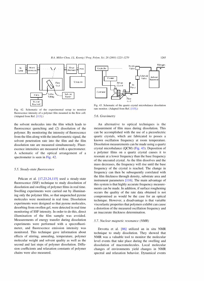
the solvent molecules into the film which leads to

fluorescence quenching and (2) dissolution of the

polymer. By monitoring the intensity of fluorescence

from the film along with the interferometric signal, the

solvent penetration rate into the film and the film

dissolution rate are measured simultaneously. Fluor-

escence intensities are measured with a spectrometer.

A schematic of the optical arrangement of a

spectrometer is seen in Fig. 42.

5.5. Steady-state fluorescence

Pekcan et al. [17,23,24,115] used a steady-state

fluorescence (SSF) technique to study dissolution of

dissolution and swelling of polymer films in real time.

Swelling experiments were carried out by illuminat-

ing only the polymer film, so that unquenched pyrene

molecules were monitored in real time. Dissolution

experiments were designed so that pyrene molecules,

desorbing from swollen gel, were detected in real time

monitoring of SSF intensity. In order to do this, direct

illumination of the film sample was avoided.

Measurements of energy transfer during dissolution

experiments were performed with a specrofluori-

meter, and fluorescence emission intensity was

monitored. This technique gave information about

effects of stirring, annealing, temperature, polymer

molecular weight and solvent quality as well as the

second and last steps of polymer dissolution. Diffu-

sion coefficients and relaxation constants of polymer

chains were also measured.

5.6. Gravimetry

An alternative to optical techniques is the

measurement of film mass during dissolution. This

can be accomplished with the use of a piezoelectric

quartz crystals, which are fabricated to posses a

known oscillation frequency at room temperature.

Dissolution measurements can be made using a quartz

crystal microbalance (QCM) (Fig. 43). Deposition of

a polymer films on a quartz crystal causes it to

resonate at a lower frequency than the base frequency

of the uncoated crystal. As the film dissolves and the

mass decreases, the frequency will rise until the base

frequency of the crystal is reached. The change in

frequency can then be subsequently correlated with

the film thickness through density, substrate area and

instrument parameters [116]. The main advantage of

this system is that highly accurate frequency measure-

ments can be made. In addition, if surface roughening

occurs the quality of the rate data obtained is not

compromised as would be the case for an optical

technique. However, a disadvantage is that variable

viscoelastic properties that polymers exhibit can cause

a distortion of the measured oscillation frequency and

an inaccurate thickness determination.

5.7. Nuclear magnetic resonance (NMR)

Devotta et al. [86] utilized an in situ NMR

technique to study dissolution. They showed that

NMR was a valuable tool to monitor the molecular

level events that take place during the swelling and

dissolution of macromolecules. Local molecular

changes of environments yield changes in NMR

spectral and relaxation behavior. Dynamical events

Fig. 42. Schematic of the experimental setup to monitor

fluorescence intensity of a polymer film mounted in the flow cell.


Fig. 43. Schematic of the quartz crystal microbalance dissolution

rate monitor. (Adapted from Ref. [115].)


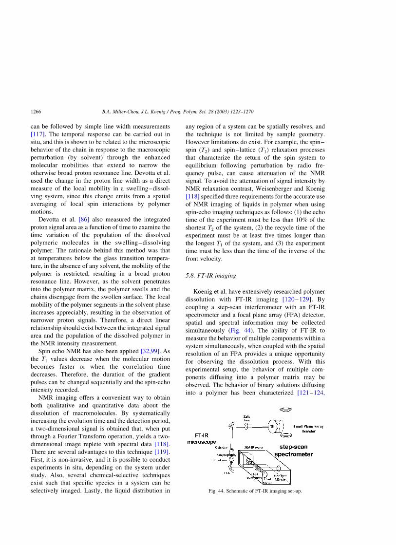
can be followed by simple line width measurements

[117]. The temporal response can be carried out in

situ, and this is shown to be related to the microscopic

behavior of the chain in response to the macroscopic

perturbation (by solvent) through the enhanced

molecular mobilities that extend to narrow the

otherwise broad proton resonance line. Devotta et al.

used the change in the proton line width as a direct

measure of the local mobility in a swelling–dissol-

ving system, since this change emits from a spatial

averaging of local spin interactions by polymer

motions.

Devotta et al. [86] also measured the integrated

proton signal area as a function of time to examine the

time variation of the population of the dissolved

polymeric molecules in the swelling–dissolving

polymer. The rationale behind this method was that

at temperatures below the glass transition tempera-

ture, in the absence of any solvent, the mobility of the

polymer is restricted, resulting in a broad proton

resonance line. However, as the solvent penetrates

into the polymer matrix, the polymer swells and the

chains disengage from the swollen surface. The local

mobility of the polymer segments in the solvent phase

increases appreciably, resulting in the observation of

narrower proton signals. Therefore, a direct linear

relationship should exist between the integrated signal

area and the population of the dissolved polymer in

the NMR intensity measurement.

Spin echo NMR has also been applied [32,99]. As

the T1 values decrease when the molecular motion

becomes faster or when the correlation time

decreases. Therefore, the duration of the gradient

pulses can be changed sequentially and the spin-echo

intensity recorded.

NMR imaging offers a convenient way to obtain

both qualitative and quantitative data about the

dissolution of macromolecules. By systematically

increasing the evolution time and the detection period,

a two-dimensional signal is obtained that, when put

through a Fourier Transform operation, yields a two-

dimensional image replete with spectral data [118].

There are several advantages to this technique [119].

First, it is non-invasive, and it is possible to conduct

experiments in situ, depending on the system under

study. Also, several chemical-selective techniques

exist such that specific species in a system can be

selectively imaged. Lastly, the liquid distribution in

any region of a system can be spatially resolves, and

the technique is not limited by sample geometry.

However limitations do exist. For example, the spin–

spin ðT2Þ and spin–lattice ðT1Þ relaxation processes

that characterize the return of the spin system to

equilibrium following perturbation by radio fre-

quency pulse, can cause attenuation of the NMR

signal. To avoid the attenuation of signal intensity by

NMR relaxation contrast, Weisenberger and Koenig

[118] specified three requirements for the accurate use

of NMR imaging of liquids in polymer when using

spin-echo imaging techniques as follows: (1) the echo

time of the experiment must be less than 10% of the

shortest T2 of the system, (2) the recycle time of the

experiment must be at least five times longer than

the longest T1 of the system, and (3) the experiment

time must be less than the time of the inverse of the

front velocity.

5.8. FT-IR imaging

Koenig et al. have extensively researched polymer

dissolution with FT-IR imaging [120–129]. By

coupling a step-scan interferometer with an FT-IR

spectrometer and a focal plane array (FPA) detector,

spatial and spectral information may be collected

simultaneously (Fig. 44). The ability of FT-IR to

measure the behavior of multiple components within a

system simultaneously, when coupled with the spatial

resolution of an FPA provides a unique opportunity

for observing the dissolution process. With this

experimental setup, the behavior of multiple com-

ponents diffusing into a polymer matrix may be

observed. The behavior of binary solutions diffusing

into a polymer has been characterized [121–124,

Fig. 44. Schematic of FT-IR imaging set-up.


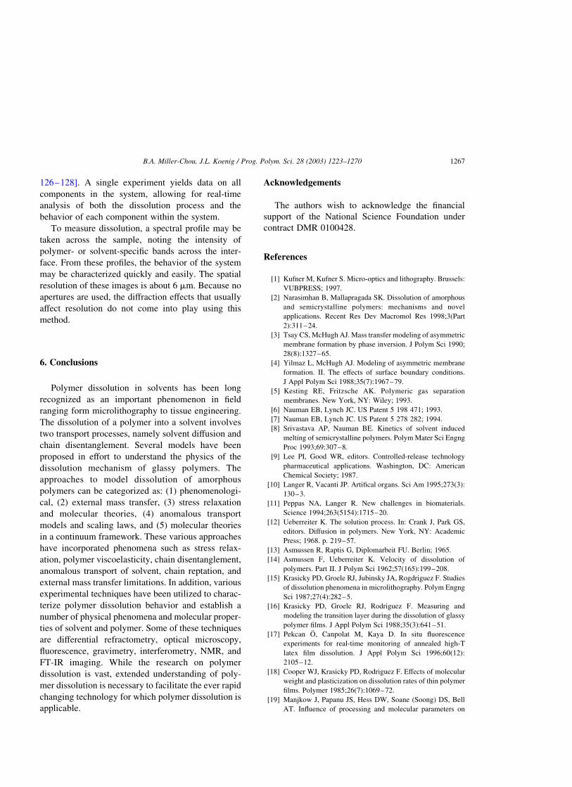
126–128]. A single experiment yields data on all

components in the system, allowing for real-time

analysis of both the dissolution process and the

behavior of each component within the system.

To measure dissolution, a spectral profile may be

taken across the sample, noting the intensity of

polymer- or solvent-specific bands across the inter-

face. From these profiles, the behavior of the system

may be characterized quickly and easily. The spatial

resolution of these images is about 6 mm. Because no

apertures are used, the diffraction effects that usually

affect resolution do not come into play using this

method.

6. Conclusions

Polymer dissolution in solvents has been long

recognized as an important phenomenon in field

ranging form microlithography to tissue engineering.

The dissolution of a polymer into a solvent involves

two transport processes, namely solvent diffusion and

chain disentanglement. Several models have been

proposed in effort to understand the physics of the

dissolution mechanism of glassy polymers. The

approaches to model dissolution of amorphous

polymers can be categorized as: (1) phenomenologi-

cal, (2) external mass transfer, (3) stress relaxation

and molecular theories, (4) anomalous transport

models and scaling laws, and (5) molecular theories

in a continuum framework. These various approaches

have incorporated phenomena such as stress relax-

ation, polymer viscoelasticity, chain disentanglement,

anomalous transport of solvent, chain reptation, and

external mass transfer limitations. In addition, various

experimental techniques have been utilized to charac-

terize polymer dissolution behavior and establish a

number of physical phenomena and molecular proper-

ties of solvent and polymer. Some of these techniques

are differential refractometry, optical microscopy,

fluorescence, gravimetry, interferometry, NMR, and

FT-IR imaging. While the research on polymer

dissolution is vast, extended understanding of poly-

mer dissolution is necessary to facilitate the ever rapid

changing technology for which polymer dissolution is

applicable.

Acknowledgements

The authors wish to acknowledge the financial

support of the National Science Foundation under

contract DMR 0100428.

References

[1] Kufner M, Kufner S. Micro-optics and lithography. Brussels:

VUBPRESS; 1997.

[2] Narasimhan B, Mallapragada SK. Dissolution of amorphous

and semicrystalline polymers: mechanisms and novel

applications. Recent Res Dev Macromol Res 1998;3(Part

2):311–24.

[3] Tsay CS, McHugh AJ. Mass transfer modeling of asymmetric

membrane formation by phase inversion. J Polym Sci 1990;

28(8):1327–65.

[4] Yilmaz L, McHugh AJ. Modeling of asymmetric membrane

formation. II. The effects of surface boundary conditions.

J Appl Polym Sci 1988;35(7):1967–79.

[5] Kesting RE, Fritzsche AK. Polymeric gas separation

membranes. New York, NY: Wiley; 1993.

[6] Nauman EB, Lynch JC. US Patent 5 198 471; 1993.

[7] Nauman EB, Lynch JC. US Patent 5 278 282; 1994.

[8] Srivastava AP, Nauman BE. Kinetics of solvent induced

melting of semicrystalline polymers. Polym Mater Sci Engng

Proc 1993;69:307–8.

[9] Lee PI, Good WR, editors. Controlled-release technology

pharmaceutical applications. Washington, DC: American

Chemical Society; 1987.

[10] Langer R, Vacanti JP. Artifical organs. Sci Am 1995;273(3):

130–3.

[11] Peppas NA, Langer R. New challenges in biomaterials.

Science 1994;263(5154):1715–20.

[12] Ueberreiter K. The solution process. In: Crank J, Park GS,

editors. Diffusion in polymers. New York, NY: Academic

Press; 1968. p. 219–57.

[13] Asmussen R, Raptis G, Diplomarbeit FU. Berlin; 1965.

[14] Asmussen F, Ueberreiter K. Velocity of dissolution of

polymers. Part II. J Polym Sci 1962;57(165):199–208.

[15] Krasicky PD, Groele RJ, Jubinsky JA, Rogdriguez F. Studies

of dissolution phenomena in microlithography. Polym Engng

Sci 1987;27(4):282–5.

[16] Krasicky PD, Groele RJ, Rodriguez F. Measuring and

modeling the transition layer during the dissolution of glassy

polymer films. J Appl Polym Sci 1988;35(3):641–51.

[17] Pekcan O, Canpolat M, Kaya D. In situ fluorescence

experiments for real-time monitoring of annealed high-T

latex film dissolution. J Appl Polym Sci 1996;60(12):

2105–12.

[18] Cooper WJ, Krasicky PD, Rodriguez F. Effects of molecular

weight and plasticization on dissolution rates of thin polymer

films. Polymer 1985;26(7):1069–72.

[19] Manjkow J, Papanu JS, Hess DW, Soane (Soong) DS, Bell

AT. Influence of processing and molecular parameters on


the dissolution rate of poly-(methyl methacrylate) thin films.

J Electrochem Soc 1987;134(8):2003–7.

[20] Papanu JS, Hess DW, Bell AT, Soane DS. Dissolution of thin

poly(methyl methacrylate) films in ketones, binary ketone/

alcohol mixtures, and hydroxy ketones. J Electrochem Soc

1989;136(10):3077–83.

[21] Papanu JS, Hess DW, Soane (Soong) DS, Bell AT. Swelling

of poly(methyl methacrylate) thin films in low molecular

weight alcohols. J Appl Polym Sci 1990;39(4):803–23.

[22] Parsonage EE, Peppas NA, Lee PI. Properties of positive

resists. II. Dissolution characteristics of irradiated poly

(methyl methacrylate) and poly(methyl methacrylate-co-

maleic anhydride). J Vac Sci Technol 1987;B5(2):

538–45.

[23] Pekcan O, Ugur S, Yilmaz Y. Real-time monitoring of

swelling and dissolution of poly(methyl methacrylate) discs

using fluorescence probes. Polymer 1997;38(9):2183–9.

[24] Pekcan O, Ugur S. Molecular weight effect on polymer

dissolution: a steady state fluorescence study. Polymer 2002;

43(6):1937–41.

[25] Ouano AC, Carothers FA. Dissolution dynamics of some

polymers: solvent–polymer boundaries. Polym Engng Sci

1980;20(2):160–6.

[26] Gipstein E, Ouano AC, Johnson DE, Need III OU.

Parameters affecting the sensitivity of poly(methyl metha-

crylate) as a positive lithographic resist. Polym Engng Sci

1977;17(6):396–401.

[27] Groele RJ, Rodriguez F. Dissolution rates of polymers and

copolymers based on methyl, ethyl, and butyl methacrylate.

J Coat Technol 1989;61(774):55–8.

[28] Reinhardt M, Pfeiffer K, Lorkowski H-J. Polymer dissol-

ution. 1. On the dissolution behavior of copolymers of methyl

methacrylate and methacrylic acid. J Appl Polym Sci 1994;

51(2):297–301.

[29] Ouano AC. Dissolution kinetics of polymers: effect of

residual solvent content. In: Seymour R, Stahl GA, editors.

Macromolecular solutions: solvent–property relationships in

polymers. New York, NY: Permagon Press; 1982.

[30] Cooper WJ, Krasicky PD, Rodriguez FJ. Dissolution rates of

poly(methyl methacrylate) films in mixed solvents. Appl

Polym Sci 1986;31(1):65–73.

[31] Manjkow J, Papanu JS, Soong DS, Hess SW, Bell AT. An in

situ study of dissolution and swelling behavior of poly-

(methyl methacrylate) thin films in solvent/nonsolvent binary

mixtures. J Appl Phys 1987;62(2):682–8.

[32] Mao S-Z, Feng H-Q. Study of the dissolution process of

polystyrene in concentrated cyclohexane solution by NMR

relaxation. Colloid Polym Sci 1998;276(3):247–51.

[33] Rodriguez F, Krasicky PD, Groele RJ. Dissolution rate

measurements. Solid State Technol 1985;28(5):125–31.

[34] Harland RS, Gazzaniga A, Sangani ME, Colombo P, Peppas

NA. Drug–polymer matrix swelling and dissolution. Phar-

maceut Res 1988;5(8):488–94.

[35] Rao V, Hinsberg WD, Frank CW, Pease RFW. The influence

of sensitizer spatial distribution on the dissolution mechan-

ism of diazonaphthoquinone resists. Proc. SPIE 1992;

1672(Adv Resist Technol Process IX):214–30.

[36] Parsonage EE, Peppas NA. Properties of positive resists. 1.

Irradiation-induced degradation and sensitivity of certain

methyl methacrylate copolymers. Br Polym J 1987;19(5):

469–77.

[37] Drummond R, Boydston GL, Peppas NA. Properties of

positive resists. III. The dissolution behavior of poly(methyl

methacrylate-co-maleic anhydride). J Appl Polym Sci 1990;

39(11/12):2267–77.

[38] Hansen CM. Hanson solubility parameters: a user’s hand-

book. Boca Raton, FL: CRC Press; 2000.

[39] Grulke EA. Solubility parameter values. In: Brandrup J,

Immergut EH, Grulke EA,, editors, 4th ed. Polymer hand-

book, vol. 7. New York, NY: Wiley; 1999. p. 675–714.

[40] Bicerano J. Prediction of polymer properties, 1st ed. New

York, NY: Marcel Dekker; 1993.

[41] Sanchez IC. Statistical thermodynamics of polymer blends.

In: Paul DR, Newman S, editors. Polymer blends. New York,

NY: Academic Press; 1978. p. 115–39.

[42] Kaelble DH. Computer aided design of polymers and

composites. New York, NY: Marcel Dekker; 1985.

[43] Fedors RF. A method for estimating both the solubility

parameters and molar volumes of liquids. Polym Engng Sci

1974;14(2):147–54.

[44] Hwang S-T, Kammermeyer K. Membranes in separations.

Malabar: Robert E. Krieger Publishing Company; 1984.

[45] Sears JK, Darby JR. The technology of plasticizers. New

York, NY: Wiley; 1982.

[46] Gardon JL. Relationship between cohesive energy densities

of polymers and Zisman’s critical surface tensions. J Phys

Chem 1963;67(9):1935–6.

[47] Girifalco LA, Good RJ. A theory for the estimation of surface

and interfacial energies. I. Derivation and application to

interfacial tension. J Phys Chem 1957;61(6):904–9.

[48] Good RJ. Estimation of surface and interfacial energies. VI.

Surface energies of some fluorocarbon surfaces from contact

angle measurements. Adv Chem Ser 1964;43:74–87.

[49] Lee LH. Relationships between surface wettability and glass

temperatures of high polymers. J Appl Polym Sci 1968;12(4):

719–30.

[50] Hildebrand JH, Scott RL. The solubility of nonelectrolytes,

3rd ed. New York, NY: Dover Publications; 1964.

[51] Gardon JL. Variables and interpretation of some destructive

cohesion and adhesion tests. In: Patrick RL, editor. Treatise

on adhesion and adhesives. New York, NY: Marcel Dekker;

1967.

[52] Hayes RA. The relationship between glass temperature,

molar cohesion, and polymer structure. J Appl Polym Sci

1961;5(15):318–21.

[53] Hildebrand JH. Study of the action of alkali on certain zinc

salts by means of the hydrogen electrode. J Am Chem Soc

1916;38(4):785–8.

[54] Scatchard G. Equilibria in nonelectrolyte solutions in relation

to the vapor pressures and densities of the components. Chem

Rev 1931;8(2):321–33.

[55] Scatchard G. Equilibrium in nonelectrolyte mixtures. Chem

Rev 1949;44(1):7–35.

[56] Burrel H. Official Digest 1955;27:726.


[57] Beerbower A. Environmental capability of liquid lubricants.

In: Interdisciplinary approach to liquid lubricant technology.

NASA Publication SP-318; 1973. p. 365–431.

[58] Watson KM. Prediction of critical temperatures and heats of

vaporization. Ind Engng Chem 1931;23:360–4.

[59] Watson KM. Thermodynamics of the liquid state. General-

ized prediction of properties. Ind Engng Chem 1943;35:

398–406.

[60] Blanks RF, Prausnitz JM. Thermodynamics of polymer

solubility in polar and nonpolar systems. Ind Engng Chem

Fundam 1964;3(1):1–8.

[61] Hansen CM. Solubility parameters. In: Koleske JV, editor.

Paint testing manual, manual 17. Philadelphia, PA: American

Society for Testing and Materials; 1995. p. 383–404.

[62] Hansen CM, Skaarup K. III. Independent calculation of the

parameter components. J Paint Technol 1967;39(511):

511–4.

[63] Hansen CM, Beerbower A. Solubility parameters. In:

Standen A, editor. Kirk–Othmer encyclopedia of chemical

technology, 3rd ed. New York, NY: Wiley; 1971. p.

889–910.

[64] Dunkel MZ. Calculation of intermolecular forces in organic

compounds. Phys Chem 1928;138:42–54.

[65] Small PA. Some factors affecting the solubility of polymers.

J Appl Chem 1953;3:71–80.

[66] Rheineck AE, Lin KF. Solubility parameter calculations

based on group contributions. J Paint Technol 1968;40(527):

611–6.

[67] Hoy KL. New values of the solubility parameters from vapor

pressure data. J Paint Technol 1970;42(541):76–118.

[68] Haggenmacher JE. The heat of vaporization as a function of

pressure and temperature. J Am Chem Soc 1946;68(8):

1633–4.

[69] Van Krevelen DW, Hoftzyer PJ. Properties of polymers: their

correlation with chemical structure; their numerical esti-

mation and prediction from additive group contributions, 3rd

ed. Amsterdam: Elsevier; 1990.

[70] Van Krevelen DW. Chemical structure and properties of

coal. XXVIII. Coal constitution and solvent extraction. Fuel

1965;44(4):229–42.

[71] Painter P, Coleman M. Fundamentals of polymer science,

2nd ed. Lancaster, PA: Technomic Publishing Co; 1997.

[72] Burke J. AIC Book and Paper Group Annual 1984;3:13.

[73] Crowley JD, Teague Jr GS, Lowe Jr JW. A three-dimensional

approach to solubility. J Paint Technol 1966;38(496):

269–80.

[74] Crowley JD, Teague Jr GS, Lowe Jr JW. A three-dimensional

approach to solubility. II. J Paint Technol 1967;39(504):

19–27.

[75] Hansen CM. 14th International Conference on Coating.

Copenhagen: Community and Care; 1994.

[76] Prigogine I. The molecular theory of solutions. Amsterdam:

North-Holland; 1957. with collaboration of Bellemans A,

Mathot A.

[77] Hansen CM, Just L. Prediction of environmental stress

cracking in plastics with Hansen solubility parameters. Ind

Engng Chem Res 2001;40(1):21–5.

[78] Teas JP. Graphic analysis of resin solubilities. J Paint Tech

1968;40(516):19–25.

[79] Barton AFM. Handbook of solubility parameters and other

cohesion parameters. Boca Raton, FL: CRC Press; 1991.

[80] Narasimhan B. Mathematical models describing polymer

dissolution: consequences for drug delivery. Adv Drug Deliv

Rev 2001;48(2/3):195–210.

[81] Narasimhan B, Peppas NA. The physics of polymer

dissolution: modeling approaches and experimental beha-

vior. Adv Polym Sci 1997;128:158–207.

[82] Ribar T. FT-IR imaging of the dissolution of poly(a-

methystyrene) in solvent mixtures and spectroscopic analysis

of vapor diffusion through an aniline oligomer chemical

sensor. Master’s Thesis, Case Western Reserve Univeristy,

2001.

[83] Tu Y-O, Ouano AC. Model for the kinematics of polymer

dissolution. IBM J Res Develop 1977;21(2):131–42.

[84] Devotta I, Ambeskar VD, Mandhare AB, Mashelkar RA. The

life time of a dissolving polymeric particle. Chem Engng Sci

1994;49(5):645–54.

[85] Ranade VV, Mashelkar RA. Convective diffusion from a

dissolving polymeric particle. AIChE J 1995;41(3):666–76.

[86] Devotta I, Badiger MV, Rajamohanan PR, Ganapathy S,

Mashelkar RA. Unusual retardation and enhancement in

polymer dissolution: role of disengagement dynamics. Chem

Engng Sci 1995;50(16):2557–69.

[87] Zielinski JM, Duda JL. Predicting polymer/solvent diffusion

coefficients using free-volume theory. AIChE J 1992;38(3):

405–15.

[88] Devotta I, Mashelkar RA. Role of thermodynamic and

kinetic factors in polymer dissolution in mixed solvents.

Chem Engng Commun 1996;156:31–45.

[89] Papanu JS, Soane (Soong) DS, Bell AT, Hess DW. Transport

models for swelling and dissolution of thin polymer films.

J Appl Polym Sci 1989;38(5):859–85.

[90] Siepmann J, Gopferich A. Mathematical modeling of

bioerodible, polymeric drug delivery systems. Adv Drug

Deliv Rev 2001;48(2/3):229–47.

[91] Siepmann J, Kranz H, Bodmeier R, Peppas NA. HPMC-

matrices for controlled drug delivery: a new model

combining diffusion, swelling, and dissolution mechanisms

and predicting the release kinetics. Pharm Res 1999;16(11):

1748–56.

[92] Siepmann J, Paeratakul O, Bodmeier R. Modeling plasticizer

uptake in aqueous polymer dispersions. Int J Pharm 1998;

165(2):191–200.

[93] Narasimhan B, Peppas NA. Molecular analysis of drug

delivery systems controlled by dissolution of the polymer

carrier. J Pharm Sci 1997;86(3):297–304.

[94] Lee PI, Peppas NA. Prediction of polymer dissolution in

swellable controlled-release systems. J Contr Rel 1987;6:

207–15.

[95] Lee H-R, Lee Y-D. Mathematical models and experiments

for swelling phenomena before dissolution of polymer films.

Chem Engng Sci 1991;46(7):1771–9.

[96] Brochard F, de Gennes PG. Kinetics of polymer dissolution.

Phys Chem Hydrodynam 1983;4(4):313–22.


[97] Herman MF, Edwards SF. A repetition model for polymer

dissolution. Macromolecules 1990;23(15):3662–71.

[98] de Gennes PG. Scaling concepts in polymer physics. Ithaca,

NY: Cornell University Press; 1979.

[99] Peppas NA, Wu JC, von Meerwal ED. Mathematical

modeling and experimental characterization of polymer

dissolution. Macromolecules 1994;27(20):5626–38.

[100] de Gennes PG, Leger L. Dynamics of entangled polymer

chains. Annu Rev Phys Chem 1982;33:49–61.

[101] de Gennes PG. Repetition of a polymer chain in the presence

of fixed obstacles. J Chem Phys 1971;55(2):572–9.

[102] Edwards SF. Statistical mechanics of polymerized material.

Proc Phys Soc 1967;92(1):9–16.

[103] Wu JC, Peppas NA. Numerical simulation of anomalous

penetrant diffusion in polymers. Appl Polym Sci 1993;

49(10):1845–56.

[104] Vrentas JS, Vrentas CM. Dissolution of rubbery and glassy

polymers. J Polym Sci, B, Polym Phys 1998;36(14):

2607–14.

[105] Narasimhan B, Peppas NA. Disentanglement and repetition

during the dissolution of rubbery polymers. J Polym Sci, B,

Polym Phys 1996;34(5):947–61.

[106] Narasimhan B, Peppas NA. On the importance of chain

repetition in models of dissolution of glassy polymers.

Macromolecules 1996;29(9):3283–91.

[107] Conte U, Colombo P, Gazzaniga A, Sangalli ME, La Manna

A. Swelling-activated drug delivery systems. Biomaterials

1988;9(6):489–93.

[108] Ju RTC, Nixon PR, Patel MV. Drug release from hydrophilic

matrices. 1. New scaling laws for predicting polymer and

drug release based on the polymer disentanglement concen-

tration and the diffusion layer. J Pharm Sci 1995;84(12):

1455–63.

[109] Ju RTC, Nixon PR, Patel MV, Tong DM. Drug release from

hydrophilic matrices. 2. A mathematical model based on the

polymer disentanglement concentration and the diffusion

layer. J Pharm Sci 1995;84(12):1464–77.

[110] Ju RTC, Nixon PR, Patel MV. Diffusion coefficients of

polymer chains in the diffusion layer adjacent to a swollen

hydrophilic matrix. J Pharm Sci 1997;86(11):1293–8.

[111] Doi M, Edwards SF. The theory of polymer dynamics, 2nd

ed. Oxford: Clarendon Press; 1986.

[112] Papanu JS, Hess DW, Bell AT, Soane DS. In situ

ellipsometry to monitor swelling and dissolution of thin

polymer films. J Electrochem Soc 1989;136(4):1195–200.

[113] McCrackin FL. Natl Bur Std, Tech Note 1969;479.

[114] Limm W, Stanton D, Dimnik GP, Winnik MA. Solvent

penetration and photoresist dissolution: a fluorescence

quenching and interferometry study. J Appl Polym Sci

1988;35(8):2099–116.

[115] Ugur S, Pekcan OJ. Fluorescence technique to study

thickness effect on dissolution of latex films. J Appl Polym

Sci 2000;77(5):1087–95.

[116] Rao V, Hinsberg WD, Frank CW, Pease RFW. Langmuier–

Blodgett deposition to evaluate dissolution behavior of

multicomponent resists. In: Thompson LF, Willson CG,

Tagawa S, editors. Polymers for microelectronics resists and

dielectrics. Washington, DC: American Chemical Society;

1994. p. 220–34.

[117] Devotta I, Premnath V, Badiger MV, Rajamohanan PR,

Ganapathy S, Mashelkar RA. On the dynamics of mobiliz-

ation in swelling-dissolving polymeric systems. Macromol-

ecules 1994;27(2):532–9.

[118] Weisenberger LA, Koenig JL. NMR imaging of solvent

diffusion in polymers. Appl Spectrosc 1989;43(7):1117–26.

[119] Hyde TM, Gladden LF, Mackley MR, Gao P. Quantitative

nuclear magnetic resonance imaging of liquids in swelling

polymers. J Polym Sci, A, Polym Chem 1995;33(11):

1795–806.

[120] Koenig J. FTIR imaging of polymer dissolution. Adv Mater

2002;14(6):457–60.

[121] Ribar T, Bhargava R, Koenig JL. FT-IR imaging of polymer

dissolution by solvent mixtures. 1. Solvents. Macromolecules

2000;33(23):8842–9.

[122] Ribar T, Koenig JL. FTIR imaging of polymer dissolution. 2.

Solvent/nonsolvent mixtures. Macromolecfsules 2001;

34(23):8340–6.

[123] Miller-Chou BA, Koenig JL. FT-IR imaging of polymer

dissolution by solvent mixtures. 3. Entangled polymer chains

with solvents. Macromolecules 2002;35(2):440–4.

[124] Miller-Chou BA, Koenig JL. Submitted for publication.



[127] Rafferty DW, Koenig JL. Submitted for publication.

[128] Rafferty DW, Koenig JL. FTIR imaging for the character-

ization of controlled-release drug delivery applications.

J Contr Rel 2002;83(1):29–39.

[129] Gonzales-Benito J, Koenig JL. FTIR imaging of the

dissolution of polymers. 4. Poly(methyl methacrylate)

using a cosolvent mixture (carbon tetrachloride/methanol).

Macromolecules 2002;35(14):7361–7.


Documents

A review of polymer dissolution - University at Buffalo · A review of polymer dissolution Beth A. Miller-Chou, Jack L. Koenig* Department of Macromolecular Science, Case School Engineering,