Embed Size (px)
Citation preview
Statistical Science2006, Vol. 21, No. 4, 552–577DOI: 10.1214/088342306000000321© Institute of Mathematical Statistics, 2006
A Review of Accelerated Test ModelsLuis A. Escobar and William Q. Meeker
Abstract. Engineers in the manufacturing industries have used acceleratedtest (AT) experiments for many decades. The purpose of AT experiments is toacquire reliability information quickly. Test units of a material, component,subsystem or entire systems are subjected to higher-than-usual levels of oneor more accelerating variables such as temperature or stress. Then the AT re-sults are used to predict life of the units at use conditions. The extrapolationis typically justified (correctly or incorrectly) on the basis of physically mo-tivated models or a combination of empirical model fitting with a sufficientamount of previous experience in testing similar units. The need to extrapo-late in both time and the accelerating variables generally necessitates the useof fully parametric models. Statisticians have made important contributionsin the development of appropriate stochastic models for AT data [typically adistribution for the response and regression relationships between the para-meters of this distribution and the accelerating variable(s)], statistical meth-ods for AT planning (choice of accelerating variable levels and allocation ofavailable test units to those levels) and methods of estimation of suitable re-liability metrics. This paper provides a review of many of the AT models thathave been used successfully in this area.
Key words and phrases: Reliability, regression model, lifetime data, degra-dation data, extrapolation, acceleration factor, Arrhenius relationship, Eyringrelationship, inverse power relationship, voltage-stress acceleration, pho-todegradation.
1. INTRODUCTION
1.1 Motivation
Today’s manufacturers face strong pressure to de-velop new, higher-technology products in record time,while improving productivity, product field reliabilityand overall quality. This has motivated the develop-ment of methods like concurrent engineering and en-couraged wider use of designed experiments for prod-uct and process improvement. The requirements forhigher reliability have increased the need for more up-front testing of materials, components and systems.This is in line with the modern quality philosophy for
Luis A. Escobar is Professor, Department of ExperimentalStatistics, Louisiana State University, Baton Rouge,Louisiana 70803, USA (e-mail: [email protected]). William Q.Meeker is Distinguished Professor, Department ofStatistics, Iowa State University, Ames, Iowa 50011, USA(e-mail: [email protected]).
producing high-reliability products: achieve high re-liability by improving the design and manufacturingprocesses; move away from reliance on inspection (orscreening) to achieve high reliability, as described inMeeker and Hamada (1995) and Meeker and Escobar(2004).
Estimating the failure-time distribution or long-termperformance of components of high-reliability prod-ucts is particularly difficult. Most modern products aredesigned to operate without failure for years, decadesor longer. Thus few units will fail or degrade appre-ciably in a test of practical length at normal use con-ditions. For example, the design and construction of acommunications satellite may allow only eight monthsto test components that are expected to be in servicefor 10 or 15 years. For such applications, AcceleratedTests (ATs) are used in manufacturing industries to as-sess or demonstrate component and subsystem relia-bility, to certify components, to detect failure modesso that they can be corrected, to compare different
552
ACCELERATED TEST MODELS 553
manufacturers, and so forth. ATs have become increas-ingly important because of rapidly changing technolo-gies, more complicated products with more compo-nents, higher customer expectations for better reliabil-ity and the need for rapid product development. Thereare difficult practical and statistical issues involved inaccelerating the life of a complicated product that canfail in different ways. Generally, information from testsat high levels of one or more accelerating variables(e.g., use rate, temperature, voltage or pressure) is ex-trapolated, through a physically reasonable statisticalmodel, to obtain estimates of life or long-term perfor-mance at lower, normal levels of the accelerating vari-able(s).
Statisticians in manufacturing industries are oftenasked to become involved in planning or analyzingdata from accelerated tests. At first glance, the statis-tics of accelerated testing appears to involve little morethan regression analysis, perhaps with a few compli-cating factors, such as censored data. The very natureof ATs, however, always requires extrapolation in theaccelerating variable(s) and often requires extrapola-tion in time. This implies critical importance of modelchoice. Relying on the common statistical practice offitting curves to data can result in an inadequate modelor even nonsense results. Statisticians working on ATprograms need to be aware of general principles of ATmodeling and current best practices.
The purpose of this review paper is to outline someof the basic ideas behind accelerated testing and espe-cially to review currently used AT modeling practiceand to describe the most commonly used AT models.In our concluding remarks we make explicit sugges-tions about the potential contributions that statisticiansshould be making to the development of AT modelsand methods. We illustrate the use of the different mod-els with a series of examples from the literature and ourown experiences.
1.2 Quantitative versus QualitativeAccelerated Tests
Within the reliability discipline, the term “acceler-ated test” is used to describe two completely differentkinds of useful, important tests that have completelydifferent purposes. To distinguish between these, theterms “quantitative accelerated tests” (QuanAT) and“qualitative accelerated tests” (QualAT) are sometimesused.
A QuanAT tests units at combinations of higher-than-usual levels of certain accelerating variables. Thepurpose of a QuanAT is to obtain information about
the failure-time distribution or degradation distributionat specified “use” levels of these variables. Generallyfailure modes of interest are known ahead of time, andthere is some knowledge available that describes therelationship between the failure mechanism and the ac-celerating variables (either based on physical/chemicaltheory or large amounts of previous experience withsimilar tests) that can be used to identify a model thatcan be used to justify the extrapolation. In this paper,we describe models for QuanATs.
A QualAT tests units at higher-than-usual combi-nations of variables like temperature cycling and vi-bration. Specific names of such tests include HALT(for highly accelerated life tests), STRIFE (stress-life)and EST (environmental stress testing). The purpose ofsuch tests is to identify product weaknesses caused byflaws in the product’s design or manufacturing process.Nelson (1990, pages 37–39) describes such tests as“elephant tests” and outlines some important issues re-lated to QualATs.
When there is a failure in a QualAT it is necessaryto find and carefully study the failure’s root cause andassess whether the failure mode could occur in actualuse or not. Knowledge and physical/chemical model-ing of the particular failure mode is useful for helpingto make this assessment. When it is determined thata failure could occur in actual use, it is necessary tochange the product design or manufacturing process toeliminate that cause of failure. Nelson (1990, page 38)describes an example where a costly effort was made toremove a high-stress-induced failure mode that neverwould have occurred in actual use.
Because the results of a QualAT are used to makechanges on the product design or manufacturing pro-cess, it is difficult, or at the very least, very risky touse the test data to predict what will happen in normaluse. Thus QualATs are generally thought of as beingnonstatistical.
1.3 Overview
The rest of this paper is organized as follows. Sec-tion 2 describes the basic physical and practical ideasbehind the use of ATs and the characteristics of variouskinds of AT data. Section 3 describes the concept ofa time-transformation model as an accelerated failure-time model, describes some commonly used specialcases and also presents several nonstandard specialcases that are important in practice. Section 4 describesacceleration models that are used when product userate is increased to get information quickly. Sections5 and 6 explain and illustrate the use of temperature
554 L. A. ESCOBAR AND W. Q. MEEKER
and humidity, respectively, to accelerate failure mech-anisms. Section 7 describes some of the special char-acteristics of ATs for photodegradation. Section 8 ex-plains and illustrates the use of increased voltage (orvoltage stress) in ATs with the commonly used inversepower relationship. This section also describes howa more general relationship, based on the Box–Coxtransformation, can be used in sensitivity analyses thathelp engineers to make decisions. Section 9 describesexamples in which combinations of two or more ac-celerating variables are used in an AT. Section 10 dis-cusses some practical concerns and general guidelinesfor conducting and interpreting ATs. Section 11 de-scribes areas of future research in the development ofaccelerated test models and the role that statisticianswill have in these developments.
2. BASIC IDEAS OF ACCELERATED TESTING
2.1 Different Types of Acceleration
The term “acceleration” has many different mean-ings within the field of reliability, but the term gener-ally implies making “time” (on whatever scale is usedto measure device or component life) go more quickly,so that reliability information can be obtained morerapidly.
2.2 Methods of Acceleration
There are different methods of accelerating a relia-bility test:
Increase the use rate of the product. This method isappropriate for products that are ordinarily not in con-tinuous use. For example, the median life of a bear-ing for a certain washing machine agitator is 12 years,based on an assumed use rate of 8 loads per week. Ifthe machine is tested at 112 loads per week (16 perday), the median life is reduced to roughly 10 months,under the assumption that the increased use rate doesnot change the cycles to failure distribution. Also, be-cause it is not necessary to have all units fail in a lifetest, useful reliability information could be obtained ina matter of weeks instead of months.
Increase the intensity of the exposure to radiation.Various types of radiation can lead to material degrada-tion and product failure. For example, organic materi-als (ranging from human skin to materials like epoxiesand polyvinyl chloride or PVC) will degrade when ex-posed to ultraviolet (UV) radiation. Electrical insula-tion exposed to gamma rays in nuclear power plantswill degrade more rapidly than similar insulation in
similar environments without the radiation. Modelingand acceleration of degradation processes by increas-ing radiation intensity is commonly done in a mannerthat is similar to acceleration by increasing use rate.
Increase the aging rate of the product. Increasingthe level of experimental variables like temperature orhumidity can accelerate the chemical processes of cer-tain failure mechanisms such as chemical degradation(resulting in eventual weakening and failure) of an ad-hesive mechanical bond or the growth of a conductingfilament across an insulator (eventually causing a shortcircuit).
Increase the level of stress (e.g., amplitude in tem-perature cycling, voltage, or pressure) under which testunits operate. A unit will fail when its strength dropsbelow applied stress. Thus a unit at a high stress willgenerally fail more rapidly than it would have failed atlow stress.
Combinations of these methods of acceleration arealso employed. Variables like voltage and tempera-ture cycling can both increase the rate of an electro-chemical reaction (thus accelerating the aging rate) andincrease stress relative to strength. In such situations,when the effect of an accelerating variable is compli-cated, there may not be enough physical knowledge toprovide an adequate physical model for acceleration(and extrapolation). Empirical models may or may notbe useful for extrapolation to use conditions.
2.3 Types of Responses
It is useful to distinguish among ATs on the basis ofthe nature of the response.
Accelerated Binary Tests (ABTs). The response inan ABT is binary. That is, whether the product hasfailed or not is the only reliability information obtainedfrom each unit. See Meeker and Hahn (1977) for an ex-ample and references.
Accelerated Life Tests (ALTs). The response in anALT is directly related to the lifetime of the prod-uct. Typically, ALT data are right-censored because thetest is stopped before all units fail. In other cases, theALT response is interval-censored because failures arediscovered at particular inspection times. See Chap-ters 2–10 of Nelson (1990) for a comprehensive treat-ment of ALTs.
Accelerated Repeated Measures Degradation Tests(ARMDTs). In an ARMDT, one measures degradation

ACCELERATED TEST MODELS 555
on a sample of units at different points in time. In gen-eral, each unit provides several degradation measure-ments. The degradation response could be actual chem-ical or physical degradation or performance degrada-tion (e.g., drop in power output). See Meeker andEscobar (1998, Chapters 13 and 21) for examples ofARMDT modeling and analysis.
Accelerated Destructive Degradation Tests(ADDTs). An ADDT is similar to an ARMDT, exceptthat the measurements are destructive, so one can ob-tain only one observation per test unit. See Escobar,Meeker, Kugler and Kramer (2003) for a discussion ofADDT methodology and a detailed case study.
These different kinds of ATs can be closely relatedbecause they can involve the same underlying physi-cal/chemical mechanisms for failure and models for ac-celeration. They are different, however, in that differentkinds of statistical models and analyses are performedbecause of the differences in the kind of response thatcan be observed.
Many of the underlying physical model assump-tions, concepts and practices are the same for ABTs,ALTs, ARMDTs and ADDTs. There are close rela-tionships among models for ABT, ALT, ARMD andADD data. Because of the different types of responses,however, the actual models fitted to the data and meth-ods of analysis differ. In some cases, analysts usedegradation-level data to define failure times. For ex-ample, turning ARMDT data into ALT data generallysimplifies analysis but may sacrifice useful informa-tion. An important characteristic of all ATs is the needto extrapolate outside the range of available data: testsare done at accelerated conditions, but estimates areneeded at use conditions. Such extrapolation requiresstrong model assumptions.
3. STATISTICAL MODELS FOR ACCELERATION
This section discusses acceleration models and somephysical considerations that lead to these models. Forfurther information on these models, see Nelson (1990,Chapter 2) and Meeker and Escobar (1998, Chap-ter 18). Other useful references include Smith (1996),Section 7 of Tobias and Trindade (1995), Sections2 and 9 of Jensen (1995) and Klinger, Nakada andMenendez (1990).
Interpretation of accelerated test data requires mod-els that relate accelerating variables like temperature,voltage, pressure, size, etc. to time acceleration. Fortesting over some range of accelerating variables, onecan fit a model to the data to describe the effect that the
variables have on the failure-causing processes. Thegeneral idea is to test at high levels of the accelerat-ing variable(s) to speed up failure processes and ex-trapolate to lower levels of the accelerating variable(s).For some situations, a physically reasonable statisticalmodel may allow such extrapolation.
Physical acceleration models. For well-understoodfailure mechanisms, one may have a model based onphysical/chemical theory that describes the failure-causing process over the range of the data and pro-vides extrapolation to use conditions. The relationshipbetween accelerating variables and the actual failuremechanism is usually extremely complicated. Often,however, one has a simple model that adequately de-scribes the process. For example, failure may resultfrom a complicated chemical process with many steps,but there may be one rate-limiting (or dominant) stepand a good understanding of this part of the processmay provide a model that is adequate for extrapolation.
Empirical acceleration models. When there is littleunderstanding of the chemical or physical processesleading to failure, it may be impossible to develop amodel based on physical/chemical theory. An empir-ical model may be the only alternative. An empiri-cal model may provide an excellent fit to the avail-able data, but provide nonsense extrapolations (e.g., thequadratic models used in Meeker and Escobar, 1998,Section 17.5). In some situations there may be exten-sive empirical experience with particular combinationsof variables and failure mechanisms and this experi-ence may provide the needed justification for extrapo-lation to use conditions.
In the rest of this section we will describe the generaltime-transformation model and some special accelera-tion models that have been useful in specific applica-tions.
3.1 General Time-Transformation Functions
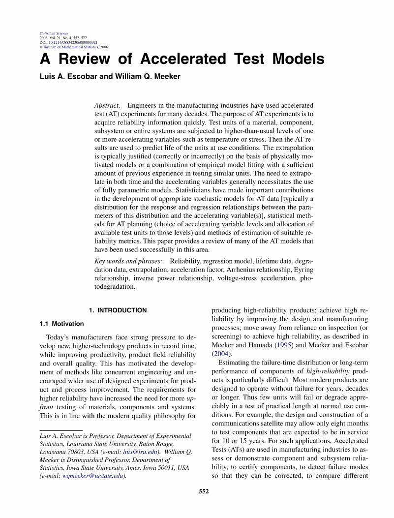
A time-transformation model maps time at one levelof x, say xU, to time at another level of x. This can beexpressed as T (x) = ϒ[T (xU),x], where xU denotesuse conditions. To be a time transformation, the func-tion ϒ(t,x) must have the following properties:
• For any x, ϒ(0,x) = 0, as in Figure 1.• ϒ(t,x) is nonnegative, that is, ϒ(t,x) ≥ 0 for all
t and x.• For fixed x, ϒ(t,x) is monotone increasing in t .• When evaluated at xU , the transformation is the
identity transformation [i.e., ϒ(t,xU) = t for all t].
556 L. A. ESCOBAR AND W. Q. MEEKER
FIG. 1. General failure-time transformation with xu < x.
A quantile of the distribution of T (x) can be deter-mined as a function of x and the corresponding quan-tile of the distribution of T (xU). In particular, tp(x) =ϒ[tp(xU),x] for 0 ≤ p ≤ 1. As shown in Figure 1,a plot of T (xU) versus T (x) can imply a particularclass of transformation functions. In particular,
• T (x) entirely below the diagonal line implies accel-eration.
• T (x) entirely above the diagonal line implies decel-eration.
• T (x) can cross the diagonal, in which case the trans-formation is accelerating over some times and de-celerating over other times. In this case the c.d.f.’sof T (x) and T (xU) cross. See Martin (1982) andLuValle, Welsher and Svoboda (1988) for furtherdiscussion of time-transformation models.
3.2 Scale-Accelerated Failure-TimeModels (SAFTs)
A simple, commonly used model used to char-acterize the effect that explanatory variables x =(x1, . . . , xk)
′ have on lifetime T is the scale-acceleratedfailure-time (SAFT) model. The model is ubiquitousin the statistical literature where it is generally re-ferred to as the “accelerated failure-time model.” Itis, however, a very special kind of accelerated failure-time model. Some of the explanatory variables in xare used for acceleration, but others may be of interest
for other reasons (e.g., for product design optimiza-tion decisions). Under a SAFT model, lifetime at x,T (x), is scaled by a deterministic factor that mightdepend on x and unknown fixed parameters. Morespecifically, a model for the random variable T (x) isSAFT if T (x) = T (xU)/AF (x), where the accelera-tion factor AF (x) is a positive function of x satisfy-ing AF (xU) = 1. Lifetime is accelerated (decelerated)when AF (x) > 1 [AF (x) < 1]. In terms of distribu-tion quantiles,
tp(x) = tp(xU)
AF (x).(1)
Some special cases of these important SAFT modelsare discussed in the following sections.
Observe that under a SAFT model, the probabil-ity that failure at conditions x occurs at or beforetime t can be written as Pr[T (x) ≤ t] = Pr[T (xU) ≤AF (x) × t]. It is common practice (but certainly notnecessary) to assume that lifetime T (x) has a log-location-scale distribution, with parameters (µ,σ ),
such as a lognormal distribution in which µ is a func-tion of the accelerating variable(s) and σ is constant(i.e., does not depend on x). In this case,
F(t;xU) = Pr[T (xU) ≤ t] = �
[log(t) − µU
σ
],
where � denotes a standard cumulative distributionfunction (e.g., standard normal) and µU is the locationparameter for the distribution of log[T (xU)]. Thus,
F(t;x) = Pr[T (x) ≤ t]= �
(log(t) − {µU − log[AF (x)]}
σ
).
Note that T (x) also has a log-location-scale distribu-tion with location parameter µ = µU − log[AF (x)]and a scale parameter σ that does not depend on x.
3.3 The Proportional Hazard Regression Model
For a continuous cdf F(t;xU) and �(x) > 0 definethe time transformation
T (x) = F−1(1 − {1 − F [T (xU);xU ]}1/�(x);xU
).
It can be shown that T (x) and T (xU) have the propor-tional hazard (PH) relationship
h(t;x) = �(x)h(t;xU).(2)
This time-transformation function is illustrated in Fig-ure 1. In this example, the amount of acceleration (ordeceleration), T (xU)/T (x), depends on the positionin time and the model is not a SAFT. If F(t;xU)
ACCELERATED TEST MODELS 557
has a Weibull distribution with scale parameter ηU
and shape parameter βU , then T (x) = T (xU)/AF (x),where AF (x) = [�(x)]1/βU . This implies that thisparticular PH regression model is also a SAFT regres-sion model. It can be shown that the Weibull distribu-tion is the only distribution in which both (1) and (2)hold. Lawless (1986) illustrates this result nicely.
3.4 Another Non-SAFT Example: The Nonconstantσ Regression Model
This section describes acceleration models with non-constant σ. In some lifetime applications, it is usefulto consider log-location-scale models in which bothµ and σ depend on explanatory variables. The log-quantile function for this model is
log[tp(x)] = µ(x) + �−1(p)σ (x).
Thustp(xU)
tp(x)= exp
{µ
(xU − µ(x)
)+ �−1(p)[σ(xU) − σ(x)]}.
Because tp(xU)/tp(x) depends on p, this model is nota SAFT model.
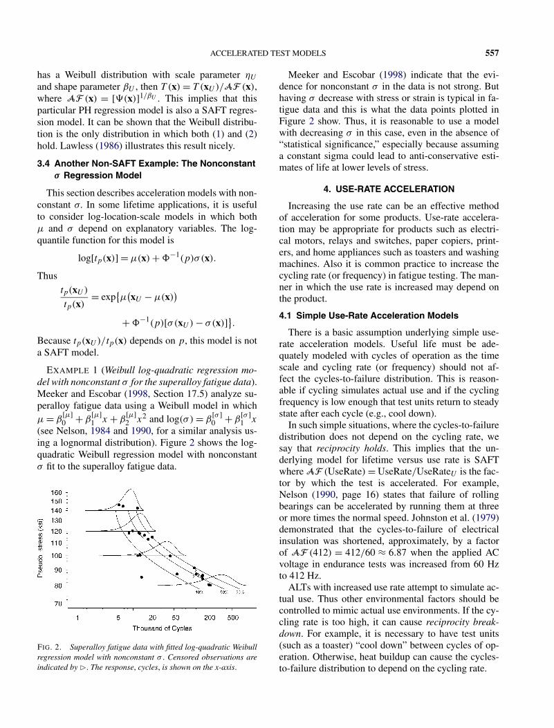
EXAMPLE 1 (Weibull log-quadratic regression mo-del with nonconstant σ for the superalloy fatigue data).Meeker and Escobar (1998, Section 17.5) analyze su-peralloy fatigue data using a Weibull model in whichµ = β
[µ]0 + β
[µ]1 x + β
[µ]2 x2 and log(σ ) = β
[σ ]0 + β
[σ ]1 x
(see Nelson, 1984 and 1990, for a similar analysis us-ing a lognormal distribution). Figure 2 shows the log-quadratic Weibull regression model with nonconstantσ fit to the superalloy fatigue data.
FIG. 2. Superalloy fatigue data with fitted log-quadratic Weibullregression model with nonconstant σ . Censored observations areindicated by �. The response, cycles, is shown on the x-axis.
Meeker and Escobar (1998) indicate that the evi-dence for nonconstant σ in the data is not strong. Buthaving σ decrease with stress or strain is typical in fa-tigue data and this is what the data points plotted inFigure 2 show. Thus, it is reasonable to use a modelwith decreasing σ in this case, even in the absence of“statistical significance,” especially because assuminga constant sigma could lead to anti-conservative esti-mates of life at lower levels of stress.
4. USE-RATE ACCELERATION
Increasing the use rate can be an effective methodof acceleration for some products. Use-rate accelera-tion may be appropriate for products such as electri-cal motors, relays and switches, paper copiers, print-ers, and home appliances such as toasters and washingmachines. Also it is common practice to increase thecycling rate (or frequency) in fatigue testing. The man-ner in which the use rate is increased may depend onthe product.
4.1 Simple Use-Rate Acceleration Models
There is a basic assumption underlying simple use-rate acceleration models. Useful life must be ade-quately modeled with cycles of operation as the timescale and cycling rate (or frequency) should not af-fect the cycles-to-failure distribution. This is reason-able if cycling simulates actual use and if the cyclingfrequency is low enough that test units return to steadystate after each cycle (e.g., cool down).
In such simple situations, where the cycles-to-failuredistribution does not depend on the cycling rate, wesay that reciprocity holds. This implies that the un-derlying model for lifetime versus use rate is SAFTwhere AF (UseRate) = UseRate/UseRateU is the fac-tor by which the test is accelerated. For example,Nelson (1990, page 16) states that failure of rollingbearings can be accelerated by running them at threeor more times the normal speed. Johnston et al. (1979)demonstrated that the cycles-to-failure of electricalinsulation was shortened, approximately, by a factorof AF (412) = 412/60 ≈ 6.87 when the applied ACvoltage in endurance tests was increased from 60 Hzto 412 Hz.
ALTs with increased use rate attempt to simulate ac-tual use. Thus other environmental factors should becontrolled to mimic actual use environments. If the cy-cling rate is too high, it can cause reciprocity break-down. For example, it is necessary to have test units(such as a toaster) “cool down” between cycles of op-eration. Otherwise, heat buildup can cause the cycles-to-failure distribution to depend on the cycling rate.
558 L. A. ESCOBAR AND W. Q. MEEKER
4.2 Cycles to Failure Depends on Use Rate
Testing at higher frequencies could shorten test timesbut could also affect the cycles-to-failure distributiondue to specimen heating or other effects. In somecomplicated situations, wear rate or degradation ratedepends on cycling frequency. Also, a product maydeteriorate in stand-by as well as during actual use.Reciprocity breakdown is known to occur, for exam-ple, for certain components in copying machines wherecomponents tend to last longer (in terms of cycles)when printing is done at higher rates. Dowling (1993,page 706) describes how increased cycle rate may af-fect the crack growth rate in per cycle fatigue testing.In such cases, the empirical power-rule relationshipAF (UseRate) = (UseRate/UseRateU)p is often used,where p can be estimated by testing at two or more userates.
EXAMPLE 2 (Increased cycling rate for low-cyclefatigue tests). Fatigue life is typically measured incycles to failure. To estimate low-cycle fatigue life ofmetal specimens, testing is done using cycling ratestypically ranging between 10 Hz and 50 Hz (where1 Hz is one stress cycle per second), depending onmaterial type and available test equipment. At 50 Hz,accumulation of 106 cycles would require about fivehours of testing. Accumulation of 107 cycles would re-quire about two days and accumulation of 108 cycleswould require about 20 days. Higher frequencies areused in the study of high-cycle fatigue.
Some fatigue tests are conducted to estimate crackgrowth rates, often as a function of explanatory vari-ables like stress and temperature. Such tests generallyuse rectangular compact tension test specimens con-taining a long slot cut normal to the centerline with achevron machined into the end of the notch. Becausethe location of the chevron is a point of highest stress,a crack will initiate and grow from there. Other fatiguetests measure cycles to failure. Such tests use cylindri-cal dog-bone-shaped specimens. Again, cracks tend toinitiate in the narrow part of the dog bone, althoughsometimes a notch is cut into the specimen to initiatethe crack.
Cycling rates in fatigue tests are generally increasedto a point where the desired response can still be mea-sured without distortion. For both kinds of fatigue tests,the results are used as inputs to engineering models thatpredict the life of actual system components. The de-tails of such models that are actually used in practiceare usually proprietary, but are typified, for example,
by Miner’s rule (e.g., page 494 of Nelson, 1990) whichuses results of tests in which specimens are tested atconstant stress to predict life in which system compo-nents are exposed to varying stresses. Example 15.3 inMeeker and Escobar (1998) describes, generally, howresults of fatigue tests on specimens are used to predictthe reliability of a jet engine turbine disk.
There is a danger, however, that increased tempera-ture due to increased cycling rate will affect the cycles-to-failure distribution. This is especially true if thereare effects like creep-fatigue interaction (see Dowling,1993, page 706, for further discussion). In another ex-ample, there was concern that changes in cycling ratewould affect the distribution of lubricant on a rollingbearing surface. In particular, if T is life in cycles andT has a log-location-scale distribution with parameters(µ,σ ), then µ = β0 + β1 log(cycles/unit time) whereβ0 and β1 can be estimated from data at two or morevalues of cycles/unit time.
5. USING TEMPERATURE TO ACCELERATEFAILURE MECHANISMS
It is sometimes said that high temperature is the en-emy of reliability. Increasing temperature is one of themost commonly used methods to accelerate a failuremechanism.
5.1 Arrhenius Relationship for Reaction Rates
The Arrhenius relationship is a widely used modelto describe the effect that temperature has on the rateof a simple chemical reaction. This relationship can bewritten as
R(temp) = γ0 exp( −Ea
k × tempK
)(3)
where R is the reaction rate, and tempK =temp °C + 273.15 is thermodynamic temperature inkelvin (K), k is either Boltzmann’s constant or theuniversal gas constant and Ea is the activation en-ergy. The parameters Ea and γ0 are product or ma-terial characteristics. In applications involving elec-tronic component reliability, Boltzmann’s constant k =8.6171 × 10−5 = 1/11605 in units of electronvolt perkelvin (eV/K) is commonly used and in this case,Ea has units of electronvolt (eV).
In the case of a simple one-step chemical reaction,Ea would represent an activation energy that quanti-fies the minimum amount of energy needed to allowa certain chemical reaction to occur. In most applica-tions involving temperature acceleration of a failuremechanism, the situation is much more complicated.
ACCELERATED TEST MODELS 559
For example, a chemical degradation process may havemultiple steps operating in series or parallel, with eachstep having its own rate constant and activation energy.Generally, the hope is that the behavior of the morecomplicated process can be approximated, over the en-tire range of temperature of interest, by the Arrheniusrelationship. This hope can be realized, for example, ifthere is a single step in the degradation process that israte-limiting and thus, for all practical purposes, con-trols the rate of the entire reaction. Of course this isa strong assumption that in most practical applicationsis impossible to verify completely. In most acceleratedtest applications, it would be more appropriate to referto Ea in (3) as a quasi-activation energy.
5.2 Arrhenius RelationshipTime-Acceleration Factor
The Arrhenius acceleration factor is
AF (temp,tempU,Ea)
= R(temp)
R(tempU)(4)
= exp[Ea
(11605
tempU K− 11605
tempK
)].
When temp> tempU , AF (temp,tempU,Ea) > 1.When tempU and Ea are understood to be, respec-tively, product use temperature and reaction-specificquasi activation energy, AF (temp) = AF (temp,
tempU,Ea) will be used to denote a time-accelerationfactor. The following example illustrates how one canassess approximate acceleration factors for a proposedaccelerated test.
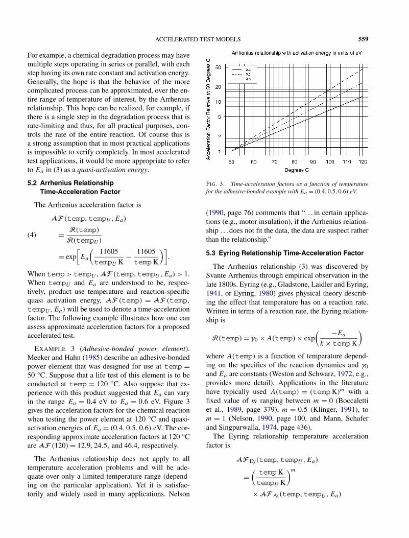
EXAMPLE 3 (Adhesive-bonded power element).Meeker and Hahn (1985) describe an adhesive-bondedpower element that was designed for use at temp =50 °C. Suppose that a life test of this element is to beconducted at temp = 120 °C. Also suppose that ex-perience with this product suggested that Ea can varyin the range Ea = 0.4 eV to Ea = 0.6 eV. Figure 3gives the acceleration factors for the chemical reactionwhen testing the power element at 120 °C and quasi-activation energies of Ea = (0.4,0.5,0.6) eV. The cor-responding approximate acceleration factors at 120 °Care AF (120) = 12.9,24.5, and 46.4, respectively.
The Arrhenius relationship does not apply to alltemperature acceleration problems and will be ade-quate over only a limited temperature range (depend-ing on the particular application). Yet it is satisfac-torily and widely used in many applications. Nelson
FIG. 3. Time-acceleration factors as a function of temperaturefor the adhesive-bonded example with Ea = (0.4,0.5,0.6) eV.
(1990, page 76) comments that “. . . in certain applica-tions (e.g., motor insulation), if the Arrhenius relation-ship . . . does not fit the data, the data are suspect ratherthan the relationship.”
5.3 Eyring Relationship Time-Acceleration Factor
The Arrhenius relationship (3) was discovered bySvante Arrhenius through empirical observation in thelate 1800s. Eyring (e.g., Gladstone, Laidler and Eyring,1941, or Eyring, 1980) gives physical theory describ-ing the effect that temperature has on a reaction rate.Written in terms of a reaction rate, the Eyring relation-ship is
R(temp) = γ0 × A(temp) × exp( −Ea
k × tempK
)
where A(temp) is a function of temperature depend-ing on the specifics of the reaction dynamics and γ0and Ea are constants (Weston and Schwarz, 1972, e.g.,provides more detail). Applications in the literaturehave typically used A(temp) = (tempK)m with afixed value of m ranging between m = 0 (Boccalettiet al., 1989, page 379), m = 0.5 (Klinger, 1991), tom = 1 (Nelson, 1990, page 100, and Mann, Schaferand Singpurwalla, 1974, page 436).
The Eyring relationship temperature accelerationfactor is
AF Ey(temp,tempU,Ea)
=(tempK
tempU K
)m
× AF Ar(temp,tempU,Ea)

560 L. A. ESCOBAR AND W. Q. MEEKER
where AF Ar(temp,tempU,Ea) is the Arrhenius ac-celeration factor from (4). For use over practical rangesof temperature acceleration, and for practical valuesof m not far from 0, the factor outside the exponen-tial has relatively little effect on the acceleration factorand the additional term is often dropped in favor of thesimpler Arrhenius relationship.
EXAMPLE 4 (Eyring acceleration factor for a metal-lization failure mode). An accelerated life test will beused to study a metallization failure mechanism for asolid-state electronic device. Experience with this typeof failure mechanism suggests that the quasi-activationenergy should be in the neighborhood of Ea = 1.2 eV.
The usual operating junction temperature for the deviceis 90 °C. The Eyring acceleration factor for testing at160 °C, using m = 1, is
AF Ey(160,90,1.2)
=(
160 + 273.15
90 + 273.15
)× AF Ar(160,90,1.2)
= 1.1935 × 491 = 586
where AF Ar(160,90,1.2) = 491 is the Arrhenius ac-celeration factor. We see that, for a fixed value of Ea ,the Eyring relationship predicts, in this case, an accel-eration that is 19% greater than the Arrhenius relation-ship. As explained below, however, this figure exagger-ates the practical difference between these models.
When fitting models to limited data, the estimateof Ea depends strongly on the assumed value for m
(e.g., 0 or 1). This dependency will compensate for andreduce the effect of changing the assumed value of m.Only with extremely large amounts of data would it bepossible to adequately separate the effects of m and Ea
using data alone. If m can be determined accurately onthe basis of physical considerations, the Eyring rela-tionship could lead to better low-stress extrapolations.Numerical evidence shows that the acceleration factorobtained from the Eyring model assuming m known,and estimating Ea from the data, is monotone decreas-ing as a function of m. Then the Eyring model givessmaller acceleration factors and smaller extrapolationto use levels of temperature when m > 0. When m < 0,Arrhenius gives a smaller acceleration factor and a con-servative extrapolation to use levels of temperature.
5.4 Reaction-Rate Acceleration for a NonlinearDegradation Path Model
Some simple chemical degradation processes (first-order kinetics) might be described by the following
path model:
D(t;temp)(5)
= D∞ × {1 − exp[−RU × AF (temp) × t]}where RU is the reaction rate at use temperaturetempU , RU × AF (temp) is the rate reaction at ageneral temperature temp, and for temp > tempU ,AF (temp) > 1. Figure 4 shows this function for fixedRU , Ea and D∞, but at different temperatures. Notefrom (5) that when D∞ > 0, D(t) is increasing andfailure occurs when D(t) > Df. For the example inFigure 4, however, D∞ < 0, D(t) is decreasing, andfailure occurs when D(t) < Df = −0.5. In either case,equating D(T ;temp) to Df and solving for failuretime gives
T (temp) = T (tempU)
AF (temp)(6)
where
T (tempU) = −(
1
RU
)log
(1 − Df
D∞
)
is failure time at use conditions. Faster degradationshortens time to any particular definition of failure(e.g., crossing Df or some other specified level) by ascale factor that depends on temperature. Thus chang-ing temperature is similar to changing the units oftime. Consequently, the time-to-failure distributions attempU and temp are related by
Pr[T (tempU) ≤ t](7)
= Pr[T (temp) ≤ t/AF (temp)].Equations (6) and (7) are forms of the scale-acceleratedfailure-time (SAFT) model introduced in Section 3.2.
FIG. 4. Nonlinear degradation paths at different temperatureswith a SAFT relationship.
ACCELERATED TEST MODELS 561
With a SAFT model, for example, if T (tempU)
(time at use or some other baseline temperature)has a log-location-scale distribution with parametersµU and σ , then
Pr[T ≤ t;tempU ] = �
[log(t) − µU
σ
].
At any other temperature,
Pr[T ≤ t;temp] = �
[log(t) − µ
σ
]where
µ = µ(x) = µU − log[AF (temp)] = β0 + β1x,
x = 11605/(tempK), xU = 11605/(tempU K), β1 =Ea and β0 = µU − β1xU . LuValle, Welsher and Svo-boda (1988) and Klinger (1992) describe more gen-eral physical/chemical degradation model characteris-tics needed to assure that the SAFT property holds.
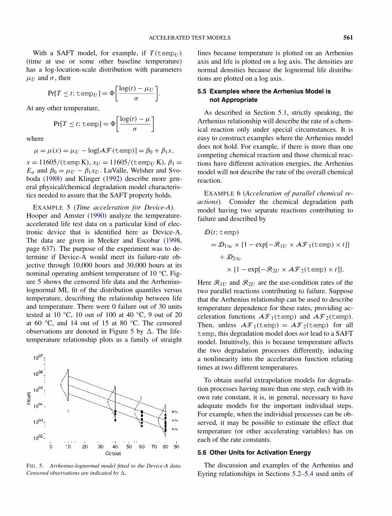
EXAMPLE 5 (Time acceleration for Device-A).Hooper and Amster (1990) analyze the temperature-accelerated life test data on a particular kind of elec-tronic device that is identified here as Device-A.The data are given in Meeker and Escobar (1998,page 637). The purpose of the experiment was to de-termine if Device-A would meet its failure-rate ob-jective through 10,000 hours and 30,000 hours at itsnominal operating ambient temperature of 10 °C. Fig-ure 5 shows the censored life data and the Arrhenius-lognormal ML fit of the distribution quantiles versustemperature, describing the relationship between lifeand temperature. There were 0 failure out of 30 unitstested at 10 °C, 10 out of 100 at 40 °C, 9 out of 20at 60 °C, and 14 out of 15 at 80 °C. The censoredobservations are denoted in Figure 5 by �. The life-temperature relationship plots as a family of straight
FIG. 5. Arrhenius-lognormal model fitted to the Device-A data.Censored observations are indicated by �.
lines because temperature is plotted on an Arrheniusaxis and life is plotted on a log axis. The densities arenormal densities because the lognormal life distribu-tions are plotted on a log axis.
5.5 Examples where the Arrhenius Model isnot Appropriate
As described in Section 5.1, strictly speaking, theArrhenius relationship will describe the rate of a chem-ical reaction only under special circumstances. It iseasy to construct examples where the Arrhenius modeldoes not hold. For example, if there is more than onecompeting chemical reaction and those chemical reac-tions have different activation energies, the Arrheniusmodel will not describe the rate of the overall chemicalreaction.
EXAMPLE 6 (Acceleration of parallel chemical re-actions). Consider the chemical degradation pathmodel having two separate reactions contributing tofailure and described by
D(t;temp)
= D1∞ × {1 − exp[−R1U × AF 1(temp) × t]}+ D2∞
× {1 − exp[−R2U × AF 2(temp) × t]}.Here R1U and R2U are the use-condition rates of thetwo parallel reactions contributing to failure. Supposethat the Arrhenius relationship can be used to describetemperature dependence for these rates, providing ac-celeration functions AF 1(temp) and AF 2(temp).Then, unless AF 1(temp) = AF 2(temp) for alltemp, this degradation model does not lead to a SAFTmodel. Intuitively, this is because temperature affectsthe two degradation processes differently, inducinga nonlinearity into the acceleration function relatingtimes at two different temperatures.
To obtain useful extrapolation models for degrada-tion processes having more than one step, each with itsown rate constant, it is, in general, necessary to haveadequate models for the important individual steps.For example, when the individual processes can be ob-served, it may be possible to estimate the effect thattemperature (or other accelerating variables) has oneach of the rate constants.
5.6 Other Units for Activation Energy
The discussion and examples of the Arrhenius andEyring relationships in Sections 5.2–5.4 used units of
562 L. A. ESCOBAR AND W. Q. MEEKER
electronvolt for Ea and electronvolt per kelvin for k.These units for the Arrhenius model are used mostcommonly in applications involving electronics. Inother areas of application (e.g., degradation of organicmaterials such as paints and coatings, plastics, foodand pharmaceuticals), it is more common to see Boltz-mann’s constant k in units of electronvolt replaced withthe universal gas constant in other units. For example,the gas constant is commonly given in units of kilo-joule per mole kelvin [i.e., R = 8.31447 kJ/(mol·K)].In this case, Ea is activation energy in units of kilo-joule per mole (kJ/mol). The corresponding Arrheniusacceleration factor is
AF (temp,tempU,Ea)
= exp[Ea
(120.27
tempU K− 120.27
tempK
)].
The universal gas constant can also be expressed inunits of kilocalorie per mole kelvin, kcal/(mol·K) [i.e.,R = 1.98588 kcal/(mol·K)]. In this case, Ea is in unitsof kilocalorie per mole (kcal/mol). The correspondingArrhenius acceleration factor is
AF (temp,tempU,Ea)
= exp[Ea
(503.56
tempU K− 503.56
tempK
)].
It is also possible to use units of kJ/(mol·K) andkcal/(mol·K) for the Ea coefficient in the Eyringmodel.
Although k is standard notation for Boltzmann’sconstant and R is standard notation for the universalgas constant, we use k to denote either of these in theArrhenius relationship.
5.7 Temperature Cycling
Some failure modes are caused by temperature cy-cling. In particular, temperature cycling causes thermalexpansion and contraction which can induce mechani-cal stresses. Some failure modes caused by thermal cy-cling include:
• Power on/off cycling of electronic equipment candamage integrated circuit encapsulement and solderjoints.
• Heat generated by take-off power-thrust in jet en-gines can cause crack initiation and growth in fandisks.
• Power-up/power-down cycles can cause cracks innuclear power plant heat exchanger tubes and tur-bine generator components.
• Temperature cycling can lead to delamination ininkjet printhead components.
As in fatigue testing, it is possible to accelerate ther-mal cycling failure modes by increasing either the fre-quency or amplitude of the cycles (increasing ampli-tude generally increases mechanical stress). The mostcommonly used model for acceleration of thermal cy-cling is the Coffin–Manson relationship which saysthat the number of cycles to failure is
N = δ
(�temp)β1
where �temp is the temperature range and δ andβ1 are properties of the material and test setup. Thispower-rule relationship explains the effect that temper-ature range has on the thermal-fatigue life cycles-to-failure distribution. Nelson (1990, page 86) suggeststhat for some metals, β1 ≈ 2 and that for plastic en-capsulements used for integrated circuits, β1 ≈ 5. TheCoffin–Manson relationship was originally developedas an empirical model to describe the effect of temper-ature cycling on the failure of components in the hotpart of a jet engine. See Nelson (1990, page 86) forfurther discussion and references.
Letting T be the random number of cycles to fail-ure (e.g., T = Nε where ε is a random variable). Theacceleration factor at �temp, relative to �tempU , is
AF (�temp) = T (�tempU)
T (�temp)=
(�temp
�tempU
)β1
.
There may be a �temp threshold below which littleor no fatigue damage is done during thermal cycling.
Empirical evidence has shown that the effect of tem-perature cycling can depend importantly ontempmax K, the maximum temperature in the cycling(e.g., if tempmax K is more than 0.2 or 0.3 times ametal’s melting point). The cycles-to-failure distribu-tion for temperature cycling can also depend on thecycling rate (e.g., due to heat buildup). An empiricalextension of the Coffin–Manson relationship that de-scribes such dependencies is
N = δ
(�temp)β1× 1
(freq)β2× exp
(Ea × 11605
tempmax K
),
where freq is the cycling frequency and Ea is a quasi-activation energy.
As with all acceleration models, caution must beused when using such a model outside the range ofavailable data and past experience.

ACCELERATED TEST MODELS 563
6. USING HUMIDITY TO ACCELERATEREACTION RATES
Humidity is another commonly used acceleratingvariable, particularly for failure mechanisms involvingcorrosion and certain kinds of chemical degradation.
EXAMPLE 7 (Accelerated life test of a printed wiringboard). Figure 6 shows data from an ALT of printedcircuit boards, illustrating the use of humidity as an ac-celerating variable. This is a subset of the larger ex-periment described by LuValle, Welsher and Mitchell(1986), involving acceleration with temperature, hu-midity and voltage. A table of the data is given inMeeker and LuValle (1995) and in Meeker and Esco-bar (1998). Figure 6 shows clearly that failures occurearlier at higher levels of humidity.
Vapor density measures the amount of water vapor ina volume of air in units of mass per unit volume. Partialvapor pressure (sometimes simply referred to as “vaporpressure”) is closely related and measures that part ofthe total air pressure exerted by the water molecules inthe air. Partial vapor pressure is approximately propor-tional to vapor density. The partial vapor pressure atwhich molecules are evaporating and condensing fromthe surface of water at the same rate is the saturationvapor pressure. For a fixed amount of moisture in theair, saturation vapor pressure increases with tempera-ture.
Relative humidity is usually defined as
RH= Vapor Pressure
Saturation Vapor Pressure
and is commonly expressed as a percent. For mostfailure mechanisms, physical/chemical theory suggests
FIG. 6. Scatterplot of printed circuit board accelerated life testdata. Censored observations are indicated by �. There are 48 cen-sored observations at 4078 hours in the 49.5% RH test and 11 cen-sored observations at 3067 hours in the 62.8% RH test.
that RH is the appropriate scale in which to relate re-action rate to humidity especially if temperature is alsoto be used as an accelerating variable (Klinger, 1991).
A variety of different humidity models (mostly em-pirical but a few with some physical basis) have beensuggested for different kinds of failure mechanisms.Much of this work has been motivated by concernsabout the effect of environmental humidity on plastic-packaged electronic devices. Humidity is also an im-portant factor in the service-life distribution of paintsand coatings. In most test applications where humidityis used as an accelerating variable, it is used in con-junction with temperature. For example, Peck (1986)presents data and models relating life of semiconduc-tor electronic components to humidity and tempera-ture. See also Peck and Zierdt (1974) and Joyce et al.(1985). Gillen and Mead (1980) describe a kinetic ap-proach for modeling accelerated aging data. LuValle,Welsher and Mitchell (1986) describe the analysis oftime-to-failure data on printed circuit boards that havebeen tested at higher than usual temperature, humid-ity and voltage. They suggest ALT models based onthe physics of failure. Chapter 2 of Nelson (1990) andBoccaletti et al. (1989) review and compare a numberof different humidity models.
The Eyring/Arrhenius temperature-humidity accel-eration relationship in the form of (14) uses x1 =11605/tempK, x2 = log(RH) and x3 = x1x2 whereRH is relative humidity, expressed as a proportion. Analternative humidity relationship suggested by Klinger(1991), on the basis of a simple kinetic model for cor-rosion, uses the term x2 = log[RH/(1−RH)] (a logistictransformation) instead.
In most applications where it is used as an acceler-ating variable, higher humidity increases degradationrates and leads to earlier failures. In applications wheredrying is the failure mechanism, however, an artificialenvironment with lower humidity can be used to accel-erate a test.
7. ACCELERATION MODEL FORPHOTODEGRADATION
Many organic compounds degrade chemically whenexposed to ultraviolet (UV) radiation. Such degrada-tion is known as photodegradation. This section de-scribes models that have been used to study pho-todegradation and that are useful when analyzing datafrom accelerated photodegradation tests. Many of theideas in this section originated from early research intothe effects of light on photographic emulsions (e.g.,

564 L. A. ESCOBAR AND W. Q. MEEKER
James, 1977) and the effect that UV exposure has oncausing skin cancer (e.g., Blum, 1959). Important ap-plications include prediction of service life of prod-ucts exposed to UV radiation (outdoor weathering) andfiber-optic systems.
7.1 Time Scale and Model for Total EffectiveUV Dosage
As described in Martin et al. (1996), the appropri-ate time scale for photodegradation is the total (i.e.,cumulative) effective UV dosage, denoted by DTot. In-tuitively, this total effective dosage can be thought ofas the cumulative number of photons absorbed intothe degrading material and that cause chemical change.The total effective UV dosage at real time t can be ex-pressed as
DTot(t) =∫ t
0DInst(τ ) dτ(8)
where the instantaneous effective UV dosage at realtime τ is
DInst(τ ) =∫ λ2
λ1
DInst(τ, λ) dλ
=∫ λ2
λ1
E0(λ, τ )(9)
× {1 − exp[−A(λ)]}φ(λ)dλ.
Here E0(λ, τ ) is the spectral irradiance (or intensity)of the light source at time τ (both artificial and naturallight sources have potentially time-dependent mixturesof light at different wavelengths, denoted by λ), [1 −exp(−A(λ))] is the spectral absorbance of the materialbeing exposed (damage is caused only by photons thatare absorbed into the material), and φ(λ) is a quasi-quantum efficiency of the absorbed radiation (allowingfor the fact that photons at certain wavelengths have ahigher probability of causing damage than others). Thefunctions E0 and A in the integrand of (9) can eitherbe measured directly or estimated from data and thefunction φ(λ) can be estimated from data. A simplelog-linear model is commonly used to describe quasi-quantum efficiency as a function of wavelength. Thatis,
φ(λ) = exp(β0 + β1λ).
The integrals over wavelength, like that in (9), are typ-ically taken over the UV-B band (290 nm to 320 nm),as this is the range of wavelengths over which bothφ(λ) and E0(λ, t) are importantly different from 0.Longer wavelengths (in the UV-A band) are not ter-ribly harmful to organic materials [φ(λ) ≈ 0]. Shorter
wavelengths (in the UV-C band) have more energy, butare generally filtered out by ozone in the atmosphere[E0(λ, t) ≈ 0].
7.2 Additivity
Implicit in the model (9) is the assumption of addi-tivity. Additivity implies, in this setting, that the photo-effectiveness of a source is equal to the sum of theeffectiveness of its spectral components. This part ofthe model makes it relatively easy to conduct exposuretests with specific combinations of wavelengths [e.g.,by using selected band-pass filters to define E0(λ, τ )
functions as levels of spectral intensity in an exper-iment] to estimate the quasi-quantum efficiency as afunction of λ. Then the total dosage model in (9) canbe used to predict photodegradation under other com-binations of wavelengths [i.e., for other E0(λ, τ ) func-tions].
7.3 Reciprocity and Reciprocity Breakdown
The intuitive idea behind reciprocity in photodegra-dation is that the time to reach a certain level ofdegradation is inversely proportional to the rate atwhich photons attack the material being degraded.Reciprocity breakdown occurs when the coefficientof proportionality changes with light intensity. Al-though reciprocity provides an adequate model forsome degradation processes (particularly when therange of intensities used in experimentation and ac-tual applications is not too broad), some examples havebeen reported in which there is reciprocity breakdown(e.g., Blum, 1959, and James, 1977).
Light intensity can be affected by filters. Sunlightis filtered by the earth’s atmosphere. In laboratoryexperiments, different neutral density filters are usedto reduce the amount of light passing to specimens(without having an important effect on the wavelengthspectrum), providing an assessment of the degree ofreciprocity breakdown. Reciprocity implies that theeffective time of exposure is
d(t) = CF × DTot(t)
= CF ×[∫ t
0
∫ λ2
λ1
DInst(τ, λ) dλdτ
]
where CF is an “acceleration factor.” For example,commercial outdoor test exposure sites use mirrors toconcentrate light to achieve, say, “5 Suns” accelerationor CF = 5. A 50% neutral density filter in a laboratoryexperiment will provide deceleration corresponding toCF = 0.5.

ACCELERATED TEST MODELS 565
When there is evidence of reciprocity breakdown,the effective time of exposure is often modeled, em-pirically, by
d(t) = (CF)p × DTot(t)(10)
= (CF)p ×[∫ t
0
∫ λ2
λ1
DInst(τ, λ) dλdτ
].
Model (10) has been shown to fit data well and exper-imental work in the photographic literature suggeststhat when there is reciprocity breakdown, the valueof p does not depend strongly, if at all, on the wave-length λ. A statistical test for p = 1 can be used toassess the reciprocity assumption.
7.4 Model for Photodegradation and UV Intensity
Degradation (or damage) D(t) at time t depends onenvironmental variables like UV, temp and RH, thatmay vary over time, say according to a multivariableprofile ξ(t) = [UV, temp,RH, . . .]. Laboratory testsare conducted in well-controlled environments, usuallyholding these variables constant (although sometimessuch variables are purposely changed during an exper-iment, as in step-stress accelerated tests). Interest of-ten centers, however, on life in a variable environment.Figure 7 shows some typical sample paths (for FTIRpeak at 1510 cm−1, representing benzene ring massloss) for several specimens of an epoxy exposed to UVradiation using a band-pass filter with a nominal centerat 306 nm. Separate paths are shown for each combi-nation of (10, 40, 60, 100)% neutral density filters and45 °C and 55 °C, as a function of total (cumulative)
absorbed UV-B dosage. These sample paths might bemodeled by a given functional form,
D(t) = g(z), z = log[d(t)] − µ,
where z is scaled time and g(z) would usually be sug-gested by knowledge of the kinetic model (e.g., linearfor zeroth-order kinetics and exponential for first-orderkinetics), although empirical curve fitting may be ade-quate for purposes where the amount of extrapolationin the time dimension is not large. As in SAFT models,µ can be modeled as a function of explanatory vari-ables like temperature and humidity when these vari-ables affect the degradation rate.
8. VOLTAGE AND VOLTAGE-STRESSACCELERATION
Increasing voltage or voltage stress (electric field) isanother commonly used method to accelerate failureof electrical materials and components like light bulbs,capacitors, transformers, heaters and insulation.
Voltage quantifies the amount of force needed tomove an electric charge between two points. Physi-cally, voltage can be thought of as the amount of pres-sure behind an electrical current. Voltage stress quanti-fies voltage per unit of thickness across a dielectric andis measured in units of volt/thickness (e.g., V/mm orkV/mm).
8.1 Voltage Acceleration Mechanisms
Depending on the failure mode, higher voltage stresscan:
FIG. 7. Sample paths for wave number 1510 cm−1 and band-pass filter with nominal center at 306 nm for different combinations oftemperature (45 and 55 °C) and neutral density filter [passing (10, 40, 60 and 100)% of photons across the UV-B spectrum].
566 L. A. ESCOBAR AND W. Q. MEEKER
• accelerate failure-causing electrochemical reactionsor the growth of failure-causing discontinuities inthe dielectric material.
• increase the voltage stress relative to dielectricstrength of a specimen. Units at higher stress willtend to fail sooner than those at lower stress.
Sometimes one or the other of these effects will be theprimary cause of failure. In other cases, both effectswill be important.
EXAMPLE 8 (Accelerated life test of insulation forgenerator armature bars). Doganaksoy, Hahn andMeeker (2003) discuss an ALT for a new mica-basedinsulation design for generator armature bars (GABs).Degradation of an organic binder in the insulationcauses a decrease in voltage strength and this wasthe primary cause of failure in the insulation. The in-sulation was designed for use at a voltage stress of120 V/mm. Voltage-endurance tests were conductedon 15 electrodes at each of five accelerated voltage lev-els between 170 V/mm and 220 V/mm (i.e., a totalof 75 electrodes). Each test was run for 6480 hours atwhich point 39 of the electrodes had not yet failed. Ta-ble 1 gives the data from these tests. The insulationengineers were interested in the 0.01 and 0.05 quan-tiles of lifetime at the use condition of 120 V/mm.Figure 8 plots the insulation lifetimes against voltagestress.
8.2 Inverse Power Relationship
The inverse power relationship is frequently used todescribe the effect that stresses like voltage and pres-sure have on lifetime. Voltage is used in the followingdiscussion. When the thickness of a dielectric mater-ial or insulation is constant, voltage is proportional tovoltage stress. Let volt denote voltage and let voltU
be the voltage at use conditions. The lifetime at stress
FIG. 8. GAB insulation data. Scatterplot of life versus voltage.Censored observations are indicated by �.
level volt is given by
T (volt) = T (voltU)
AF (volt)=
(volt
voltU
)β1
T (voltU)
where β1, in general, is negative. The model has SAFTform with acceleration factor
AF (volt) = AF (volt,voltU,β1)
= T (voltU)
T (volt)(11)
=(volt
voltU
)−β1
.
If T (voltU) has a log-location-scale distribution withparameters µU and σ , then T (volt) also has a log-location-scale distribution with µ = β0 + β1x, wherexU = log(voltU), x = log(volt), β0 = µU − β1xU
and σ does not depend on x.
EXAMPLE 9 (Time acceleration for GAB insula-tion). For the GAB insulation data in Example 8,an estimate for β1 is β̂1 = −9 (methods for com-puting such estimates are described in Meeker and
TABLE 1GAB insulation data
Voltage stress Lifetime(V/mm) (thousand hours)
170 15 censoreda
190 3.248, 4.052, 5.304, 12 censoreda
200 1.759, 3.645, 3.706, 3.726, 3.990, 5.153, 6.368, 8 censoreda
210 1.401, 2.829, 2.941, 2.991, 3.311, 3.364, 3.474, 4.902, 5.639, 6.021, 6.456, 4 censoreda
220 0.401, 1.297, 1.342, 1.999, 2.075, 2.196, 2.885, 3.019, 3.550, 3.566, 3.610, 3.659, 3.687, 4.152, 5.572
aUnits were censored at 6.480 thousand hours.
ACCELERATED TEST MODELS 567
FIG. 9. Time-acceleration factor as a function of voltage stressand exponent −β1 = −7,−9,−11.
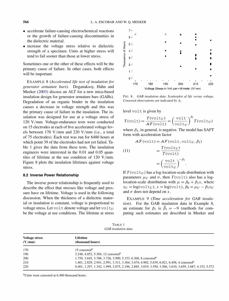
Escobar, 1998, Chapter 19). Recall that the designvoltage stress is voltU = 120 V/mm and considertesting at volt = 170 V/mm. Thus, using β1 = β̂1,AF (170) = (170/120)9 ≈ 23. Thus by increasingvoltage stress from 120 V/mm to 170 V/mm, oneestimates that lifetime is shortened by a factor of1/AF (170) ≈ 1/23 = 0.04. Figure 9 plots AF ver-sus volt for β1 = −7,−9,−11. Using direct compu-tations or from the plot, one obtains AF (170) ≈ 11for β1 = −7 and AF (170) ≈ 46 for β1 = −11.
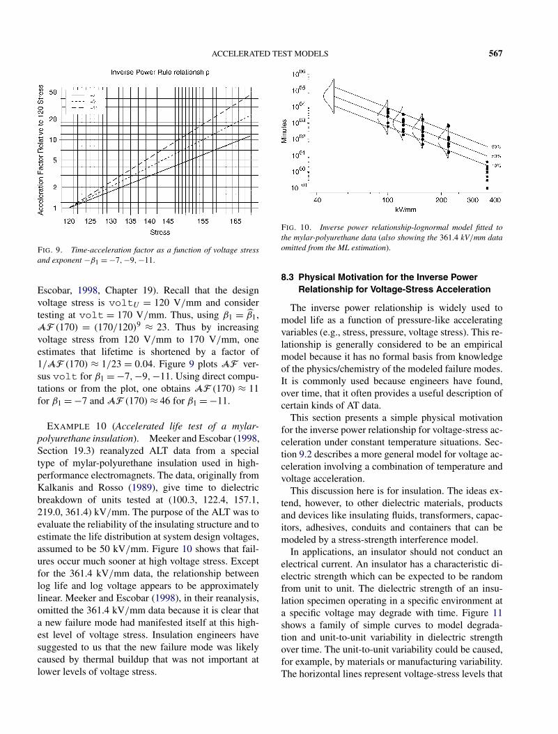
EXAMPLE 10 (Accelerated life test of a mylar-polyurethane insulation). Meeker and Escobar (1998,Section 19.3) reanalyzed ALT data from a specialtype of mylar-polyurethane insulation used in high-performance electromagnets. The data, originally fromKalkanis and Rosso (1989), give time to dielectricbreakdown of units tested at (100.3, 122.4, 157.1,219.0, 361.4) kV/mm. The purpose of the ALT was toevaluate the reliability of the insulating structure and toestimate the life distribution at system design voltages,assumed to be 50 kV/mm. Figure 10 shows that fail-ures occur much sooner at high voltage stress. Exceptfor the 361.4 kV/mm data, the relationship betweenlog life and log voltage appears to be approximatelylinear. Meeker and Escobar (1998), in their reanalysis,omitted the 361.4 kV/mm data because it is clear thata new failure mode had manifested itself at this high-est level of voltage stress. Insulation engineers havesuggested to us that the new failure mode was likelycaused by thermal buildup that was not important atlower levels of voltage stress.
FIG. 10. Inverse power relationship-lognormal model fitted tothe mylar-polyurethane data (also showing the 361.4 kV/mm dataomitted from the ML estimation).
8.3 Physical Motivation for the Inverse PowerRelationship for Voltage-Stress Acceleration
The inverse power relationship is widely used tomodel life as a function of pressure-like acceleratingvariables (e.g., stress, pressure, voltage stress). This re-lationship is generally considered to be an empiricalmodel because it has no formal basis from knowledgeof the physics/chemistry of the modeled failure modes.It is commonly used because engineers have found,over time, that it often provides a useful description ofcertain kinds of AT data.
This section presents a simple physical motivationfor the inverse power relationship for voltage-stress ac-celeration under constant temperature situations. Sec-tion 9.2 describes a more general model for voltage ac-celeration involving a combination of temperature andvoltage acceleration.
This discussion here is for insulation. The ideas ex-tend, however, to other dielectric materials, productsand devices like insulating fluids, transformers, capac-itors, adhesives, conduits and containers that can bemodeled by a stress-strength interference model.
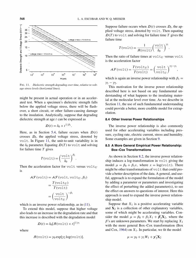
In applications, an insulator should not conduct anelectrical current. An insulator has a characteristic di-electric strength which can be expected to be randomfrom unit to unit. The dielectric strength of an insu-lation specimen operating in a specific environment ata specific voltage may degrade with time. Figure 11shows a family of simple curves to model degrada-tion and unit-to-unit variability in dielectric strengthover time. The unit-to-unit variability could be caused,for example, by materials or manufacturing variability.The horizontal lines represent voltage-stress levels that
568 L. A. ESCOBAR AND W. Q. MEEKER
FIG. 11. Dielectric strength degrading over time, relative to volt-age-stress levels (horizontal lines).
might be present in actual operation or in an acceler-ated test. When a specimen’s dielectric strength fallsbelow the applied voltage stress, there will be flash-over, a short circuit, or other failure-causing damageto the insulation. Analytically, suppose that degradingdielectric strength at age t can be expressed as
D(t) = δ0 × t1/β1 .
Here, as in Section 5.4, failure occurs when D(t)
crosses Df, the applied voltage stress, denoted byvolt. In Figure 11, the unit-to-unit variability is inthe δ0 parameter. Equating D(T ) to volt and solvingfor failure time T gives
T (volt) =(volt
δ0
)β1
.
Then the acceleration factor for volt versus voltU
is
AF (volt) = AF (volt,voltU,β1)
= T (voltU)
T (volt)
=(volt
voltU
)−β1
which is an inverse power relationship, as in (11).To extend this model, suppose that higher voltage
also leads to an increase in the degradation rate and thatthis increase is described with the degradation model
D(t) = δ0[R(volt) × t]1/γ1
where
R(volt) = γ0 exp[γ2 log(volt)].
Suppose failure occurs when D(t) crosses Df, the ap-plied voltage stress, denoted by volt. Then equatingD(T ) to volt and solving for failure time T gives thefailure time
T (volt) = 1
R(volt)
(volt
δ0
)γ1
.
Then the ratio of failure times at voltU versus voltis the acceleration factor
AF (volt) = T (voltU)
T (volt)=
(volt
voltU
)γ2−γ1
,
which is again an inverse power relationship with β1 =γ1 − γ2.
This motivation for the inverse power relationshipdescribed here is not based on any fundamental un-derstanding of what happens to the insulating mater-ial at the molecular level over time. As we describe inSection 11, the use of such fundamental understandingcould provide a better, more credible model for extrap-olation.
8.4 Other Inverse Power Relationships
The inverse power relationship is also commonlyused for other accelerating variables including pres-sure, cycling rate, electric current, stress and humidity.Some examples are given in Section 9.
8.5 A More General Empirical Power Relationship:Box–Cox Transformations
As shown in Section 8.2, the inverse power relation-ship induces a log-transformation in volt giving themodel µ = β0 + β1x, where x = log(volt). Theremight be other transformations of volt that could pro-vide a better description of the data. A general, and use-ful, approach is to expand the formulation of the modelby adding a parameter or parameters and investigatingthe effect of perturbing the added parameter(s), to seethe effect on answers to questions of interest. Here thisapproach is used to expand the inverse power relation-ship model.
Suppose that X1 is a positive accelerating variableand X2 is a collection of other explanatory variables,some of which might be accelerating variables. Con-sider the model µ = β0 + β1X1 + β ′
2X2, where theβ’s are unknown parameters. We start by replacing X1with the more general Box–Cox transformation (Boxand Cox, 1964) on X1. In particular, we fit the model
µ = γ0 + γ1W1 + γ ′2X2
ACCELERATED TEST MODELS 569
where the γ ’s are unknown parameters and
W1 =
Xλ1 − 1
λ, λ �= 0,
log(X1), λ = 0.(12)
The Box–Cox transformation (Box and Cox, 1964)was originally proposed as a simplifying transforma-tion for a response variable. Transformation of accel-erating and explanatory variables, however, providesa convenient extension of the accelerating modelingchoices. The Box–Cox transformation includes all thepower transformations and because W1 is a continuousfunction of λ, (12) provides a continuum of transfor-mations for possible evaluation and model assessment.The Box–Cox transformation parameter λ can be var-ied over some range of values (e.g., −1 to 2) to see theeffect of different voltage-life relationships on the fit-ted model and inferences of interest. The results fromthe analysis can be displayed in a number of differentways.
For fixed X2, the Box–Cox transformation model ac-celeration factor is
AF BC(X1) =
[exp
(Xλ
1U − Xλ1
λ
)]γ1
, if λ �= 0,(X1U
X1
)γ1
, if λ = 0,
where X1U are use conditions for the X1 acceleratingvariable. AF BC(X1) is monotone increasing in X1 ifγ1 < 0 and monotone decreasing in X1 if γ1 > 0.
EXAMPLE 11 (Spring life test data). Meeker, Es-cobar and Zayac (2003) analyze spring acceleratedlife test data. Time is in units of kilocycles to failure.The explanatory variables are processing temperature(Temp) in degrees Fahrenheit, spring compression dis-placement (Stroke) in mils, and the categorical variableMethod which takes the values New or Old. Springsthat had not failed after 5000 kilocycles were codedas “Suspended.” At the condition 50 mils, 500 °F andthe New processing method, there were no failures be-fore 5000 kilocycles. All of the other conditions had atleast some failures, and at five of the twelve conditionsall of the springs failed. At some of the conditions, oneor more of the springs had not failed after 5000 kilocy-cles.
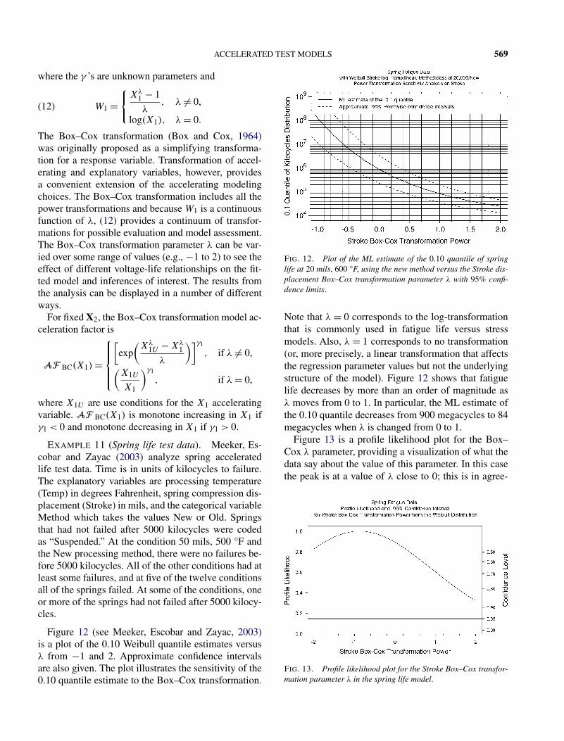
Figure 12 (see Meeker, Escobar and Zayac, 2003)is a plot of the 0.10 Weibull quantile estimates versusλ from −1 and 2. Approximate confidence intervalsare also given. The plot illustrates the sensitivity of the0.10 quantile estimate to the Box–Cox transformation.
FIG. 12. Plot of the ML estimate of the 0.10 quantile of springlife at 20 mils, 600 °F, using the new method versus the Stroke dis-placement Box–Cox transformation parameter λ with 95% confi-dence limits.
Note that λ = 0 corresponds to the log-transformationthat is commonly used in fatigue life versus stressmodels. Also, λ = 1 corresponds to no transformation(or, more precisely, a linear transformation that affectsthe regression parameter values but not the underlyingstructure of the model). Figure 12 shows that fatiguelife decreases by more than an order of magnitude asλ moves from 0 to 1. In particular, the ML estimate ofthe 0.10 quantile decreases from 900 megacycles to 84megacycles when λ is changed from 0 to 1.
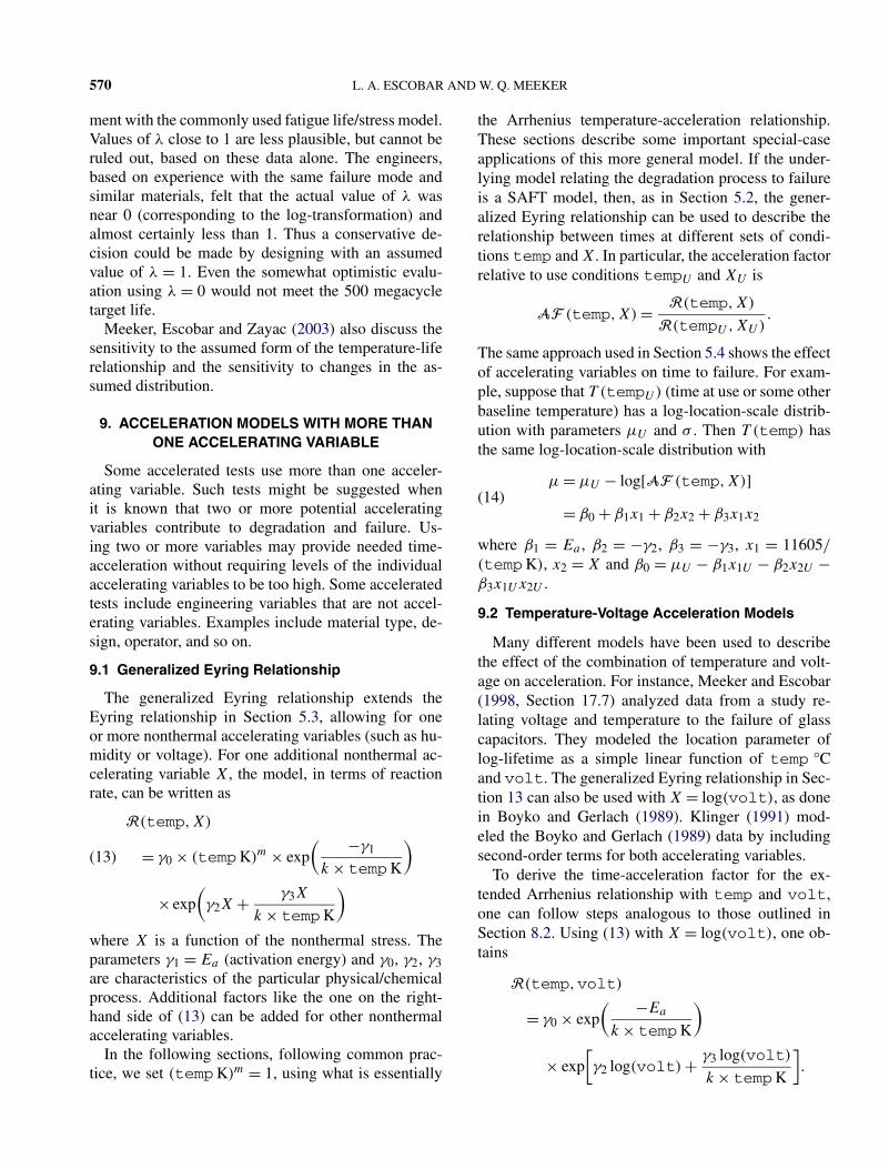
Figure 13 is a profile likelihood plot for the Box–Cox λ parameter, providing a visualization of what thedata say about the value of this parameter. In this casethe peak is at a value of λ close to 0; this is in agree-
FIG. 13. Profile likelihood plot for the Stroke Box–Cox transfor-mation parameter λ in the spring life model.
570 L. A. ESCOBAR AND W. Q. MEEKER
ment with the commonly used fatigue life/stress model.Values of λ close to 1 are less plausible, but cannot beruled out, based on these data alone. The engineers,based on experience with the same failure mode andsimilar materials, felt that the actual value of λ wasnear 0 (corresponding to the log-transformation) andalmost certainly less than 1. Thus a conservative de-cision could be made by designing with an assumedvalue of λ = 1. Even the somewhat optimistic evalu-ation using λ = 0 would not meet the 500 megacycletarget life.
Meeker, Escobar and Zayac (2003) also discuss thesensitivity to the assumed form of the temperature-liferelationship and the sensitivity to changes in the as-sumed distribution.
9. ACCELERATION MODELS WITH MORE THANONE ACCELERATING VARIABLE
Some accelerated tests use more than one acceler-ating variable. Such tests might be suggested whenit is known that two or more potential acceleratingvariables contribute to degradation and failure. Us-ing two or more variables may provide needed time-acceleration without requiring levels of the individualaccelerating variables to be too high. Some acceleratedtests include engineering variables that are not accel-erating variables. Examples include material type, de-sign, operator, and so on.
9.1 Generalized Eyring Relationship
The generalized Eyring relationship extends theEyring relationship in Section 5.3, allowing for oneor more nonthermal accelerating variables (such as hu-midity or voltage). For one additional nonthermal ac-celerating variable X, the model, in terms of reactionrate, can be written as
R(temp,X)
= γ0 × (tempK)m × exp( −γ1
k × tempK
)(13)
× exp(γ2X + γ3X
k × tempK
)
where X is a function of the nonthermal stress. Theparameters γ1 = Ea (activation energy) and γ0, γ2, γ3are characteristics of the particular physical/chemicalprocess. Additional factors like the one on the right-hand side of (13) can be added for other nonthermalaccelerating variables.
In the following sections, following common prac-tice, we set (tempK)m = 1, using what is essentially
the Arrhenius temperature-acceleration relationship.These sections describe some important special-caseapplications of this more general model. If the under-lying model relating the degradation process to failureis a SAFT model, then, as in Section 5.2, the gener-alized Eyring relationship can be used to describe therelationship between times at different sets of condi-tions temp and X. In particular, the acceleration factorrelative to use conditions tempU and XU is
AF (temp,X) = R(temp,X)
R(tempU,XU).
The same approach used in Section 5.4 shows the effectof accelerating variables on time to failure. For exam-ple, suppose that T (tempU) (time at use or some otherbaseline temperature) has a log-location-scale distrib-ution with parameters µU and σ . Then T (temp) hasthe same log-location-scale distribution with
µ = µU − log[AF (temp,X)](14)
= β0 + β1x1 + β2x2 + β3x1x2
where β1 = Ea , β2 = −γ2, β3 = −γ3, x1 = 11605/
(tempK), x2 = X and β0 = µU − β1x1U − β2x2U −β3x1Ux2U .
9.2 Temperature-Voltage Acceleration Models
Many different models have been used to describethe effect of the combination of temperature and volt-age on acceleration. For instance, Meeker and Escobar(1998, Section 17.7) analyzed data from a study re-lating voltage and temperature to the failure of glasscapacitors. They modeled the location parameter oflog-lifetime as a simple linear function of temp °Cand volt. The generalized Eyring relationship in Sec-tion 13 can also be used with X = log(volt), as donein Boyko and Gerlach (1989). Klinger (1991) mod-eled the Boyko and Gerlach (1989) data by includingsecond-order terms for both accelerating variables.
To derive the time-acceleration factor for the ex-tended Arrhenius relationship with temp and volt,one can follow steps analogous to those outlined inSection 8.2. Using (13) with X = log(volt), one ob-tains
R(temp,volt)
= γ0 × exp( −Ea
k × tempK
)
× exp[γ2 log(volt) + γ3 log(volt)
k × tempK
].
ACCELERATED TEST MODELS 571
Again, failure occurs when the dielectric strengthcrosses the applied voltage stress, that is, D(t) =volt. This occurs at time
T (temp,volt) = 1
R(temp,volt)
(volt
δ0
)γ1
.
From this, one computes
AF (temp,volt)
= T (tempU,voltU)
T (temp,volt)
= exp[Ea(x1U − x1)] ×(volt
voltU
)γ2−γ1
× {exp[x1 log(volt) − x1U log(voltU)]}γ3,
where x1U = 11605/(tempU K) and x1 = 11605/
(tempK). When γ3 = 0, there is no interaction be-tween temperature and voltage. In this case,AF (temp,volt) can be factored into two terms, onethat involves temperature only and another term that in-volves voltage only. Thus, if there is no interaction, thecontribution of temperature (voltage) to acceleration isthe same at all levels of voltage (levels of temperature).
9.3 Temperature-Current DensityAcceleration Models
d’Heurle and Ho (1978) and Ghate (1982) studiedthe effect of increased current density (A/cm2) on
electromigration in microelectronic aluminum conduc-tors. High current densities cause atoms to move morerapidly, eventually causing extrusion or voids that leadto component failure. ATs for electromigration oftenuse increased current density and temperature to ac-celerate the test. An extended Arrhenius relationshipcould be appropriate for such data. In particular, whenT has a log-location-scale distribution, then (13) ap-plies with x1 = 11605/tempK, x2 = log(current).The model with β3 = 0 (without interaction) is knownas “Black’s equation” (Black, 1969).
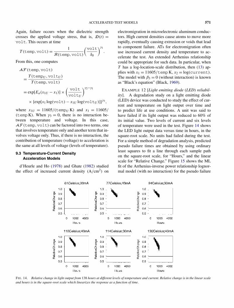
EXAMPLE 12 [Light emitting diode (LED) reliabil-ity]. A degradation study on a light emitting diode(LED) device was conducted to study the effect of cur-rent and temperature on light output over time andto predict life at use conditions. A unit was said tohave failed if its light output was reduced to 60% ofits initial value. Two levels of current and six levelsof temperature were used in the test. Figure 14 showsthe LED light output data versus time in hours, in thesquare-root scale. No units had failed during the test.For a simple method of degradation analysis, predictedpseudo failure times are obtained by using ordinaryleast squares to fit a line through each sample pathon the square-root scale, for “Hours,” and the linearscale for “Relative Change.” Figure 15 shows the MLfit of the Arrhenius-inverse power relationship lognor-mal model (with no interaction) for the pseudo failure
FIG. 14. Relative change in light output from 138 hours at different levels of temperature and current. Relative change is in the linear scaleand hours is in the square-root scale which linearizes the response as a function of time.
572 L. A. ESCOBAR AND W. Q. MEEKER
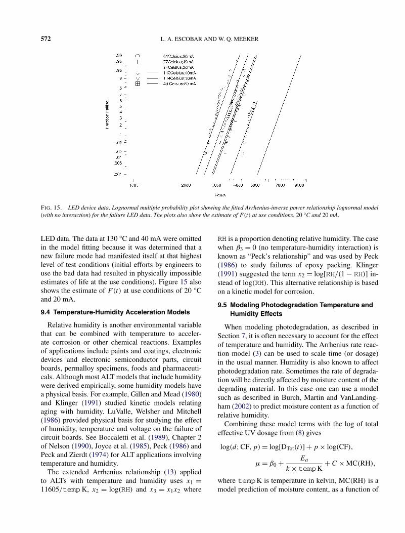
FIG. 15. LED device data. Lognormal multiple probability plot showing the fitted Arrhenius-inverse power relationship lognormal model(with no interaction) for the failure LED data. The plots also show the estimate of F(t) at use conditions, 20 °C and 20 mA.
LED data. The data at 130 °C and 40 mA were omittedin the model fitting because it was determined that anew failure mode had manifested itself at that highestlevel of test conditions (initial efforts by engineers touse the bad data had resulted in physically impossibleestimates of life at the use conditions). Figure 15 alsoshows the estimate of F(t) at use conditions of 20 °Cand 20 mA.
9.4 Temperature-Humidity Acceleration Models
Relative humidity is another environmental variablethat can be combined with temperature to acceler-ate corrosion or other chemical reactions. Examplesof applications include paints and coatings, electronicdevices and electronic semiconductor parts, circuitboards, permalloy specimens, foods and pharmaceuti-cals. Although most ALT models that include humiditywere derived empirically, some humidity models havea physical basis. For example, Gillen and Mead (1980)and Klinger (1991) studied kinetic models relatingaging with humidity. LuValle, Welsher and Mitchell(1986) provided physical basis for studying the effectof humidity, temperature and voltage on the failure ofcircuit boards. See Boccaletti et al. (1989), Chapter 2of Nelson (1990), Joyce et al. (1985), Peck (1986) andPeck and Zierdt (1974) for ALT applications involvingtemperature and humidity.
The extended Arrhenius relationship (13) appliedto ALTs with temperature and humidity uses x1 =11605/tempK, x2 = log(RH) and x3 = x1x2 where
RH is a proportion denoting relative humidity. The casewhen β3 = 0 (no temperature-humidity interaction) isknown as “Peck’s relationship” and was used by Peck(1986) to study failures of epoxy packing. Klinger(1991) suggested the term x2 = log[RH/(1 − RH)] in-stead of log(RH). This alternative relationship is basedon a kinetic model for corrosion.
9.5 Modeling Photodegradation Temperature andHumidity Effects
When modeling photodegradation, as described inSection 7, it is often necessary to account for the effectof temperature and humidity. The Arrhenius rate reac-tion model (3) can be used to scale time (or dosage)in the usual manner. Humidity is also known to affectphotodegradation rate. Sometimes the rate of degrada-tion will be directly affected by moisture content of thedegrading material. In this case one can use a modelsuch as described in Burch, Martin and VanLanding-ham (2002) to predict moisture content as a function ofrelative humidity.
Combining these model terms with the log of totaleffective UV dosage from (8) gives
log(d;CF,p) = log[DTot(t)] + p × log(CF),
µ = β0 + Ea
k × tempK+ C × MC(RH),
where tempK is temperature in kelvin, MC(RH) is amodel prediction of moisture content, as a function of
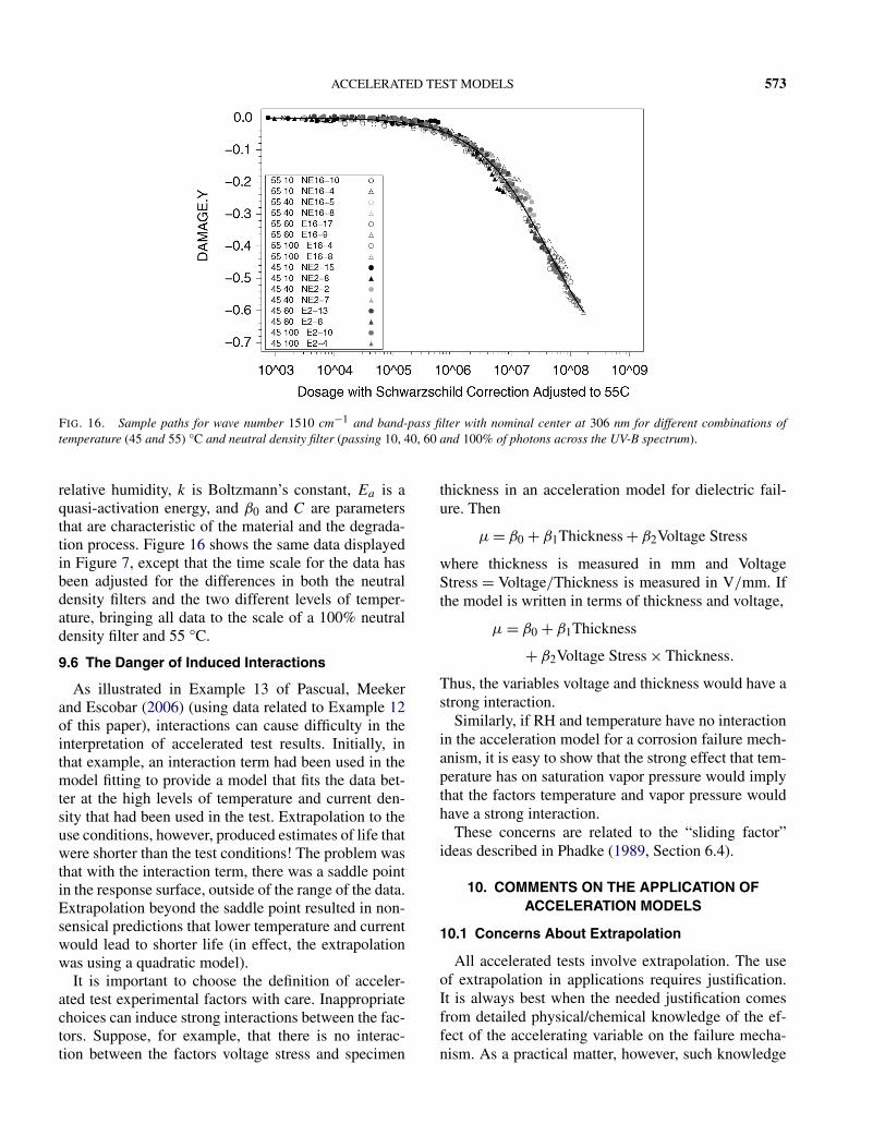
ACCELERATED TEST MODELS 573
FIG. 16. Sample paths for wave number 1510 cm−1 and band-pass filter with nominal center at 306 nm for different combinations oftemperature (45 and 55) °C and neutral density filter (passing 10, 40, 60 and 100% of photons across the UV-B spectrum).
relative humidity, k is Boltzmann’s constant, Ea is aquasi-activation energy, and β0 and C are parametersthat are characteristic of the material and the degrada-tion process. Figure 16 shows the same data displayedin Figure 7, except that the time scale for the data hasbeen adjusted for the differences in both the neutraldensity filters and the two different levels of temper-ature, bringing all data to the scale of a 100% neutraldensity filter and 55 °C.
9.6 The Danger of Induced Interactions
As illustrated in Example 13 of Pascual, Meekerand Escobar (2006) (using data related to Example 12of this paper), interactions can cause difficulty in theinterpretation of accelerated test results. Initially, inthat example, an interaction term had been used in themodel fitting to provide a model that fits the data bet-ter at the high levels of temperature and current den-sity that had been used in the test. Extrapolation to theuse conditions, however, produced estimates of life thatwere shorter than the test conditions! The problem wasthat with the interaction term, there was a saddle pointin the response surface, outside of the range of the data.Extrapolation beyond the saddle point resulted in non-sensical predictions that lower temperature and currentwould lead to shorter life (in effect, the extrapolationwas using a quadratic model).
It is important to choose the definition of acceler-ated test experimental factors with care. Inappropriatechoices can induce strong interactions between the fac-tors. Suppose, for example, that there is no interac-tion between the factors voltage stress and specimen
thickness in an acceleration model for dielectric fail-ure. Then
µ = β0 + β1Thickness + β2Voltage Stress
where thickness is measured in mm and VoltageStress = Voltage/Thickness is measured in V/mm. Ifthe model is written in terms of thickness and voltage,
µ = β0 + β1Thickness
+ β2Voltage Stress × Thickness.
Thus, the variables voltage and thickness would have astrong interaction.
Similarly, if RH and temperature have no interactionin the acceleration model for a corrosion failure mech-anism, it is easy to show that the strong effect that tem-perature has on saturation vapor pressure would implythat the factors temperature and vapor pressure wouldhave a strong interaction.
These concerns are related to the “sliding factor”ideas described in Phadke (1989, Section 6.4).
10. COMMENTS ON THE APPLICATION OFACCELERATION MODELS
10.1 Concerns About Extrapolation
All accelerated tests involve extrapolation. The useof extrapolation in applications requires justification.It is always best when the needed justification comesfrom detailed physical/chemical knowledge of the ef-fect of the accelerating variable on the failure mecha-nism. As a practical matter, however, such knowledge
574 L. A. ESCOBAR AND W. Q. MEEKER
is often lacking, as are time and resources for acquiringthe needed knowledge. Empirical relationships are of-ten used as justification, but rarely are data available tocheck the relationship over the entire range of interestfor the accelerating variable(s).
Evans (1977) makes the important point that theneed to make rapid reliability assessments and the factthat accelerated tests may be “the only game in town”are not sufficient to justify the use of the method. Jus-tification must be based on physical models or empiri-cal evidence. Evans (1991) describes difficulties withaccelerated testing and suggests the use of sensitiv-ity analysis, such as that described in Meeker, Escobarand Zayac (2003). He also comments that accelerationfactors of 10 “are not unreasonable” but that “factorsmuch larger than that tend to be figments of the imagi-nation and lots of correct but irrelevant arithmetic.”
10.2 Some Basic Guidelines
Some guidelines for the use of acceleration modelsinclude:
• ATs must generate the same failure mode occurringin the field.
Generally, accelerated tests are used to obtaininformation about one particular, relatively simplefailure mechanism (or corresponding degradationmeasure). If there is more than one failure mode, it ispossible that the different failure mechanisms will beaccelerated at different rates. Then, unless this is ac-counted for in the modeling and analysis, estimatescould be seriously incorrect when extrapolating tolower use levels of the accelerating variables.
• Accelerating variables should be chosen to corre-spond with variables that cause actual failures.
• It is useful to investigate previous attempts to accel-erate failure mechanisms similar to the ones of in-terest. There are many research reports and papersthat have been published in the physics of failureliterature. The annual Proceedings of the Interna-tional Reliability Physics Symposium, sponsored bythe IEEE Electron Devices Society and the IEEE Re-liability Society, contain numerous articles describ-ing physical models for acceleration and failure.
• Accelerated tests should be designed, as much aspossible, to minimize the amount of extrapolationrequired, as described in Chapters 20 and 21 ofMeeker and Escobar (1998). High levels of accel-erating variables can cause extraneous failure modesthat would never occur at use levels of the acceler-ating variables. If extraneous failures are not recog-nized and properly handled, they can lead to seri-ously incorrect conclusions. Also, the relationship
may not be accurate enough over a wide range ofacceleration.
• In practice, it is difficult or impractical to verify ac-celeration relationships over the entire range of in-terest. Of course, accelerated test data should beused to look for departures from the assumed ac-celeration model. It is important to recognize, how-ever, that the available data will generally providevery little power to detect anything but the most seri-ous model inadequacies. Typically there is no usefuldiagnostic information about possible model inade-quacies at accelerating variable levels close to useconditions.
• Simple models with the right shape have generallyproven to be more useful than elaborate multipara-meter models.
• Sensitivity analyses should be used to assess the ef-fect of perturbing uncertain inputs (e.g., inputs re-lated to model assumptions).
• Accelerated test programs should be planned andconducted by teams including individuals knowl-edgeable about the product and its use environ-ment, the physical/chemical/mechanical aspects ofthe failure mode, and the statistical aspects of thedesign and analysis of reliability experiments.
11. FUTURE RESEARCH IN THE DEVELOPMENTOF ACCELERATED TEST MODELS
Research in the development of accelerated testmodels is a multidisciplinary activity. Statisticianshave an important role to play on the teams of scientiststhat develop and use accelerated test models. On such ateam engineers and scientists are primarily responsiblefor:
• Identifying and enumerating possible failure modesand, for new products, predicting all possible life-limiting failure modes.
• Understanding the physical/chemical failure mecha-nisms that lead to a product’s failure modes and foridentifying accelerating variables that can be used toaccelerate the failure mechanism.
• Suggesting deterministic physical/chemical mathe-matical relationships between the rate of the failuremechanisms and the accelerating variable(s). Whensuch a relationship is not available, they may be ableto provide guidance from standard practice or previ-ous experience with similar products and materials.
Statisticians are important for:
ACCELERATED TEST MODELS 575
• Planning appropriate experiments. Accelerated testprograms often start with simple experiments to un-derstand the failure modes that can occur and the be-havior of mechanisms that can cause failures. Use oftraditional methods for designed experiments is im-portant for these tests. In addition, there may be spe-cial features of accelerated tests (e.g., censoring) thatrequire special test planning methods (see Chapter 6of Nelson, 1990, and Chapter 20 of Meeker and Es-cobar, 1998, for discussion of accelerated test plan-ning).
• Providing expertise in the analysis of data aris-ing from preliminary studies and the acceleratedtests themselves. Features such as censoring, mul-tiple failure modes and models that are nonlinearin the parameters are common. Methods for de-tecting model departures are particularly important.Model departures may suggest problems with thedata, sources of experimental variability that mightbe eliminated or problems with the suggested modelthat may suggest changes to the proposed model.
• Identifying sources of variability in experimentaldata (either degradation data or life data) that reflectactual variability in the failure mechanism. For thispurpose it is generally useful to compare field data.In most applications there will be additional variabil-ity in field data and it is important to understand thedifferences in order to design appropriate laboratoryexperiments and to be able to draw useful conclu-sions and predictions from laboratory data.
• Working within cross-disciplinary teams to developstatistical models of failure and acceleration basedon fundamental understanding of failure mecha-nisms. With fundamental understanding of failuremechanisms and knowledge of sources of vari-ability, it is possible to develop, from first prin-ciples, failure-time distributions and accelerationmodels. Better, more credible, models for extrapola-tion should result from such modeling efforts if theassumptions and other inputs are accurate. Some ex-amples of where such models have been developedinclude– Fisher and Tippett (1928) derived the asymptotic
distributions of extreme values and these resultsprovide fundamental motivation for use of distri-butions such as the Weibull distribution (one ofthe three distributions of minima) in reliability ap-plications in which failure is caused by the firstof many similar possible events (e.g., the failureof a large system with many similar possible fail-ure points, none of which dominates in the failureprocess).
– Tweedie (1956), in modeling electrophoretic mea-surements, used the distribution of first passagetime of a Brownian motion with drift to derive theinverse Gaussian distribution.
– Birnbaum and Saunders (1969), in modeling timeto fracture from a fatigue crack growth process,derived a distribution that is today known as theBirnbaum–Saunders distribution. This distribu-tion can be thought of as a discrete-time analogof the inverse Gaussian distribution.
– Meeker and LuValle (1995), using a kinetic modelfor the growth of conducting filaments, developeda probability distribution, dependent on the levelof relative humidity, to predict the failure time ofprinted circuit boards.
– Meeker, Escobar and Lu (1998), using a kineticmodel for chemical degradation inside an elec-tronic amplifying device, developed a probabilitydistribution which, when combined with the Ar-rhenius model, could be used to predict the failuretime of the devices.
– LuValle et al. (1998) and LuValle, Lefevre andKannan (2004, pages 200–206) used physics-based models to describe degradation processes.
ACKNOWLEDGMENTS
We want to thank two anonymous referees who pro-vided valuable comments on an earlier version of thispaper. These comments led to important improvementsin the paper. Charles Annis and Michael LuValle pro-vided us, respectively, helpful descriptions of methodsfor fatigue testing and modeling chemical processes re-lated to ATs.
Figures 4 and 11 originally appeared in Meeker andEscobar (1998) and Figures 12 and 13 originally ap-peared in Meeker, Escobar and Zayac (2003) and ap-pear in this paper with permission of the copyrightowner, John Wiley and Sons, Inc.
REFERENCES
BIRNBAUM, Z. W. and SAUNDERS, S. C. (1969). A new familyof life distributions. J. Appl. Probab. 6 319–327 MR0253493
BLACK, J. R. (1969). Electromigration—a brief survey and somerecent results. IEEE Transactions on Electron Devices 16 338–347.
BLUM, H. F. (1959). Carcinogenesis by Ultraviolet Light. Prince-ton Univ. Press.
BOCCALETTI, G., BORRI, F. R., D’ESPONOSA, F. and GHIO, E.(1989). Accelerated tests. In Microelectronic Reliability 2. In-tegrity Assessment and Assurance (E. Pollino, ed.) Chapter 11.Artech House, Norwood, MA.
576 L. A. ESCOBAR AND W. Q. MEEKER
BOX, G. E. P. and COX, D. R. (1964). An analysis of transforma-tions (with discussion). J. Roy. Statist. Soc. Ser. B 26 211–252.MR0192611
BOYKO, K. C. and GERLACH, D. L. (1989). Time dependent di-electric breakdown of 210 Å oxides. In Proc. 27th Annual Inter-national Reliability Physics Symposium 1–8. IEEE Press, NewYork.
BURCH, D., MARTIN, J. W. and VANLANDINGHAM, M. R.(2002). Computer analysis of a polymer coating exposed to fieldweather conditions. J. Coatings Technology 74 75–86.
D’HEURLE, F. M. and HO, P. S. (1978). Electromigration in thinfilms. In Thin Films: Interdiffusion and Reactions (J. M. Poate,K. N. Tu and J. W. Mayer, eds.) 243–303. Wiley, New York.
DOWLING, N. E. (1993). Mechanical Behavior of Materials. Pren-tice Hall, Englewood Cliffs, NJ.
ESCOBAR, L. A., MEEKER, W. Q., KUGLER, D. L. andKRAMER, L. L. (2003). Accelerated destructive degradationtests: Data, models and analysis. In Mathematical and Statisti-cal Methods in Reliability (B. H. Lindqvist and K. A. Doksum,eds.) 319–337. World Scientific, River Edge, NJ. MR2031082
EVANS, R. A. (1977). Accelerated testing: The only game in town.IEEE Transactions on Reliability 26 241.
EVANS, R. A. (1991). Accelerated testing. IEEE Transactions onReliability 40 497.
EYRING, H. (1980). Basic Chemical Kinetics. Wiley, New York.FISHER, R. and TIPPETT, L. H. (1928). Limiting forms of the fre-
quency distribution of the largest and smallest member of a sam-ple. Proc. Cambridge Philos. Soc. 24 180–190.
GHATE, P. B. (1982). Electromigration-induced failures in VLSIinterconnects. In Proc. 20th Annual International ReliabilityPhysics Symposium 292–299. IEEE Press, New York.
GILLEN, K. T. and MEAD, K. E. (1980). Predicting life ex-pectancy and simulating age of complex equipment using accel-erated aging techniques. Available from the National TechnicalInformation Service, U.S. Department of Commerce, 5285 PortRoyal Road, Springfield, VA 22151.
GLASSTONE, S., LAIDLER, K. J. and EYRING, H. (1941). Theoryof Rate Processes. McGraw-Hill, New York.
HAHN, G. J., MEEKER, W. Q. and DOGANAKSOY, N. (2003).Accelerated testing for speedier reliability analysis. QualityProgress 36(6) 58–63.
HOOPER, J. H. and AMSTER, S. J. (1990). Analysis and presenta-tion of reliability data. In Handbook of Statistical Methods forEngineers and Scientists (H. M. Wadsworth, ed.). McGraw Hill,New York.
JAMES, T. H., ed. (1977). The Theory of the Photographic Process,4th ed. Macmillan, New York.
JENSEN, F. (1995). Electronic Component Reliability: Fundamen-tals, Modelling, Evaluation and Assurance. Wiley, New York.
JOHNSTON, D. R., LAFORTE, J. T., PODHOREZ, P. E. andGALPERN, H. N. (1979). Frequency acceleration of volt-age endurance. IEEE Transactions on Electrical Insulation 14121–126.
JOYCE, W. B., LIOU, K.-Y., NASH, F. R., BOSSARD, P. R. andHARTMAN, R. L. (1985). Methodology of accelerated aging.AT&T Technical J. 64 717–764.
KALKANIS, G. and ROSSO, E. (1989). The inverse power lawmodel for the lifetime of a mylar–polyurethane laminated dchv insulating structure. Nuclear Instruments and Methods inPhysics Research A281 489–496.
KLINGER, D. J. (1991). On the notion of activation energy inreliability: Arrhenius, Eyring and thermodynamics. In AnnualReliability and Maintainability Symposium 295–300. IEEE,New York.
KLINGER, D. J. (1991). Humidity acceleration factor for plasticpackaged electronic devices. Quality and Reliability Engineer-ing International 7 365–370.
KLINGER, D. J. (1992). Failure time and rate constant of degrada-tion: An argument for the inverse relationship. MicroelectronicsReliability 32 987–994.
KLINGER, D. J., NAKADA, Y. and MENENDEZ, M. A., eds.(1990). AT&T Reliability Manual. Van Nostrand Reinhold,New York.
LAWLESS, J. F. (1986). A note on lifetime regression models. Bio-metrika 73 509–512. MR0855912
LUVALLE, M. J., COPELAND, L. R., KANNAN, S., JUDKINS, J.and LEMAIRE, P. (1998). A strategy for extrapolation in accel-erated testing. Bell Labs Technical J. 3(3) 139–147.
LUVALLE, M. J., LEFEVRE, B. and KANNAN, S. (2004). Designand Analysis of Accelerated Tests for Mission Critical Reliabil-ity. Chapman and Hall/CRC, Boca Raton, FL.
LUVALLE, M. J., WELSHER, T. L. and MITCHELL, J. P. (1986).A new approach to the extrapolation of accelerated life testdata. In Proc. Fifth International Conference on Reliability andMaintainability 620–635. Biarritz, France.
LUVALLE, M. J., WELSHER, T. L. and SVOBODA, K. (1988).Acceleration transforms and statistical kinetic models. J. Statist.Phys. 52 311–330. MR0968588
MANN, N. R., SCHAFER, R. E. and SINGPURWALLA, N. D.(1974). Methods for Statistical Analysis of Reliability and LifeData. Wiley, New York.
MARTIN, J. W. (1982). Time transformation functions commonlyused in life testing analysis. Durability of Building Materials 1175–194.
MARTIN, J. W., SAUNDERS, S. C., FLOYD, F. L. and WINE-BURG, J. P. (1996). Methodologies for Predicting the ServiceLives of Coating Systems. Federation of Societies for CoatingsTechnology, Blue Bell, PA.
MEEKER, W. Q. and ESCOBAR, L. A. (1998). Statistical Methodsfor Reliability Data. Wiley, New York.
MEEKER, W. Q. and ESCOBAR, L. A. (2004). Reliability: Theother dimension of quality. Quality Technology and Quantita-tive Management 1 1–25.
MEEKER, W. Q., ESCOBAR, L. A. and LU, C. J. (1998). Accel-erated degradation tests: Modeling and analysis. Technometrics40 89–99.
MEEKER, W. Q., ESCOBAR, L. A. and ZAYAC, S. (2003). Useof sensitivity analysis to assess the effect of model uncertaintyin analyzing accelerated life test data. In Case Studies in Reli-ability and Maintenance (W. R. Blischke and D. N. PrabhakarMurthy, eds.) 135–162. Wiley, New York.
MEEKER, W. Q. and HAHN, G. J. (1977). Asymptotically opti-mum over-stress tests to estimate the survival probability at acondition with a low expected failure probability (with discus-sion). Technometrics 19 381–404.
MEEKER, W. Q. and HAHN, G. J. (1985). How to Plan an Accel-erated Life Test: Some Practical Guidelines. American Societyfor Quality Control, Milwaukee, WI.
MEEKER, W. Q. and HAMADA, M. (1995). Statistical tools for therapid development and evaluation of high-reliability products.IEEE Transactions on Reliability 44 187–198.
ACCELERATED TEST MODELS 577
MEEKER, W. Q. and LUVALLE, M. J. (1995). An acceleratedlife test model based on reliability kinetics. Technometrics 37133–146.
NELSON, W. (1984). Fitting of fatigue curves with nonconstantstandard deviation to data with runouts. J. Testing and Evalua-tion 12 69–77.
NELSON, W. (1990). Accelerated Testing: Statistical Models, TestPlans and Data Analyses. Wiley, New York.
PASCUAL, F. G., MEEKER, W. Q. and ESCOBAR, L. A. (2006).Accelerated life test models and data analysis. In Handbookof Engineering Statistics (H. Pham, ed.) Chapter 22. Springer,New York.
PECK, D. S. (1986). Comprehensive model for humidity testingcorrelation. In Proc. International Reliability Physics Sympo-sium 44–50. IEEE Press, New York.
PECK, D. S. and ZIERDT, C. H., JR. (1974). The reliability ofsemiconductor devices in the Bell System. In Proc. IEEE 62185–211.
PHADKE, M. S. (1989). Quality Engineering Using Robust De-sign. Prentice Hall, Englewood Cliffs, NJ.
SMITH, J. S. (1996). Physics of failure. In Handbook of Reli-ability Engineering and Management, 2nd ed. (W. G. Ireson,C. F. Coombs and R. Y. Moss, eds.) Chapter 14. McGraw Hill,New York.
TOBIAS, P. A. and TRINDADE, D. C. (1995). Applied Reliability,2nd ed. Van Nostrand Reinhold, New York.
TWEEDIE, M. C. K. (1956). Some statistical properties of inverseGaussian distributions. Virginia J. Sci. 7 160–165.
WESTON, R. and SCHWARZ, H. A. (1972). Chemical Kinetics.Prentice Hall, Englewood Cliffs, NJ.