Embed Size (px)
Citation preview

A retrospective look at mountain lion populations in California (1906-2018)
JUSTIN A. DELLINGER* AND STEVEN G. TORRES†
California Department of Fish and Wildlife, Wildlife Investigations Lab, 1701 Nimbus Rd, Suite
D, Rancho Cordova, CA 95670, USA
†Retired
*Corresponding Author: [email protected]
Mountain lion (Puma concolor) population management in California has varied widely
over the past 100 plus years, ranging from a bounty system (1906-1963) to specially-
protected status (1972-present). To elucidate how these different management approaches
have influenced California’s mountain lion populations, we estimated historical
population trends by combining purposeful (i.e., bounty and depredation) and incidental
(i.e., vehicle strike) mortality statistics with estimates of annual growth and mortality
rates derived from the literature. We used a backwards population projection method to
estimate annual abundance and population trends, starting with population sizes drawn
randomly from a uniform distribution ranging from 1,000-5,000. These back-calculations
suggest that the bounty was effective at reducing mountain lion populations, as all
simulations indicated a statewide population decline during this period. Specially-
protected status was also likely effective, as mountain lion populations appear to have
increased statewide following cessation of the bounty period. These analyses
demonstrate the effectiveness of various management approaches to influence mountain
lion population trends for the intended results, and provide context for understanding
historical aspects of mountain lion populations in California, which is unique from other
areas given the species’ specially-protected status here.
Key words: bounty, depredation, mortality, Puma concolor, vehicle strike

________________________________________________________________________
Mountain lion (Puma concolor) population management in California has gone through
many changes (Table 1), resulting from changing attitudes of public stakeholders, policy makers,
and elected officials (Bruskotter and Shelby 2010; Davenport et al. 2010). Mountain lions were
subject to a bounty system in California from 1906-1963 (Mansfield and Weaver 1989), with the
amount paid per mountain lion varying over time and with sex (Table 1). In 1919, the California
Department of Fish and Game (Department) employed the first full-time statewide lion hunter
(McLean 1954), and the number of individuals employed for this purpose grew to a maximum of
five in 1948. The Department employed at least one individual through 1959, prior to
terminating the bounty program in 1963 (Nowak 1974). Records show that bounty hunters took
224 mountain lions on average each year, totaling 12,580 over the duration of the bounty system
(Mansfield and Weaver 1989). After the bounty system ended in 1963, hunters could take
mountain lions year-round without a bag limit or hunting license. In 1970 the Fish and Game
Commission designated mountain lions as a game species, wherein a hunting license and tag
were required for the 1970 and 1971 hunting seasons. In 1972, the state legislature enacted a
moratorium on the hunting of mountain lions due to growing public concern over the status of
the species in California (Fitzhugh and Gorenzel 1986). The moratorium expired in 1986 and
ungulate conservation groups successfully lobbied to re-designate mountain lions as a game
species. As a result, the Department began to develop regulations for harvest quotas and
management zones, and to assess environmental impacts in compliance with the California
Endangered Species Act (Mansfield and Weaver 1989). However, a majority vote by the citizens
of California passed Proposition 117 (Fish & Game Code §4800-4809) in 1990, which classified

mountain lions as a specially-protected mammal species. This unique status was a political
designation, and not based on biological information regarding population abundance or trend.
Thus, from 1990 to present, human-caused mountain lion mortalities have been limited to
vehicle strikes, targeted removal under the authority of a depredation permit, poaching, public
safety concerns, and take of mountain lions negatively impacting California bighorn sheep
(Torres et al. 1996; Fish & G. Code §4801).
Mountain lions’ specially-protected status has resulted in a spectrum of concerns from
interested parties. On one end of the spectrum are ungulate conservation groups who have
expressed concern that the mountain lion population may be increasing and thus negatively
impacting deer (Odocoileus hemionus) herds due to high rates of predation (Proposition 197
[1996]; Walgamuth 2017). Conversely, predator conservation groups have suggested that a
combination of mortality factors (e.g., habitat loss, degradation, and fragmentation; vehicle
strikes; depredation take; disease; etc.) may be causing the state’s mountain lion population to
decline in numbers and genetic diversity to a level that may threaten the species’ viability
(Proposition 117 [1990]; Walter 2015). To address these concerns, wildlife managers and
biologists must gain insight into historical trends and the contemporary abundance of mountain
lion populations to make effective management decisions.
In light of the controversies regarding mountain lion status in California, the Department
seeks to clarify the effects of historical management on mountain lion populations. For this
purpose, we proposed the following hypotheses: 1) the statewide mountain lion population in
California declined during the bounty period (1906-1963); and 2) the statewide mountain lion
population in California increased during the period of increasing legal protections (1972-2018).
We tested these hypotheses by analyzing historical statewide data on mountain lion mortalities
within a discrete growth equation to estimate historical population trends. Our objectives were to
estimate statewide population trends during and after the bounty period, and to elucidate how
historical and current management policies have affected the statewide mountain lion population.
METHODS
Study area
We collected mortality data from California county courthouses; California Departments
of Fish and Wildlife (Department), and Transportation (Caltrans); California Highway Patrol
(CHP); and United States Department of Agriculture, Wildlife Services (USDA Wildlife
Services). County courthouse and Department records supplied data on mountain lions removed
during the bounty period, and included data from all counties except Imperial, Sacramento, San
Francisco, Solano, and Sutter, from which no bounty records were available. CHP and Caltrans
supplied statewide data on mountain lions killed due to vehicle strikes. Department and USDA
Wildlife Services supplied statewide data on mountain lions removed due to depredation.
Data collection
We collected statewide data on mountain lions purposefully killed due to bounties,
hunting, and depredations from 1906-2018 (McLean 1954; Fitzhugh and Gorenzel 1986;
Mansfield and Weaver 1989), and on mountain lions incidentally killed due to vehicle strikes
from 2009-2018 (Table 2). There were no data available on purposeful removals between the
conclusion of the bounty system in 1963 and establishment of a hunting season in 1970, nor were
accurate data available on sex and age of individuals for any animals (bountied, hunted,
depredated, vehicle-killed) but the most recent depredations (2015-2017).
For all these data, we made a number of assumptions described here, which may
variously have contributed to over- or under-estimates of the number of lions removed from the

population. Throughout the time period of interest, mountain lions undoubtedly died due to
additional human-related incidents (e.g., poaching). Because of a scarcity of accurate data on
such incidents, we assumed that our bounty, hunting, depredation, and vehicle strike data
represented the majority of human-caused mountain lion mortalities. This assumption may
underestimate the number of individuals removed. In addition, bounty systems encourage
inflated reporting (i.e., submitting animals for bounty in California while they were actually
taken in a neighboring state), so bounty data may overestimate the number of individuals
removed (Fitzhugh and Gorenzel 1986). However, it should be noted that the majority (>50%) of
the bounty records submitted were by agency employees. Further, none of the border counties
had high numbers of bounties paid relative to interior counties. As such, we assumed that these
records are accurately reported and represent animals taken within California. There is also a
likelihood that vehicle strike data are underreported. We assumed that the proportion of missing
records is similar from year-to-year and does not account for a significant number of records in a
given year. To account for potentially missing depredation reports, we compared Department
records and USDA Wildlife Services records for 1998-2018. Discrepancies between the two sets
of records were generally within ±10 individuals statewide, and occurred for a variety of reasons
(e.g., lost paperwork, position vacancies, etc.). Where discrepancies existed between the two
datasets, we used the higher of the two reported numbers to represent number of animals
removed via depredation in the given year.
Population simulations
Using a back-calculation method to estimate the historical population of mountain lions
in California, we began with a discrete growth equation, modified to include rates of human-
caused mortality:

Nt+1 = Ntλt – dt – Ntλtmt , (1)
where λ is the annual intrinsic growth rate, d is the combined number of individuals taken
purposefully and incidentally per year, and m is the coefficient of additional mortality (e.g.,
intraspecific strife, poaching, and disease) per year (Mykra and Pohja-Mykra 2015). Estimating
the trend of a population from one year to the next requires an estimate of potential annual
growth and mortality. Based on results reported by Beausoleil et al. (2013), we established the
mean intrinsic growth (λ) at 1.14 (14% annual increase) with a standard deviation of 0.03 to
allow for annual stochasticity (Robinson et al. 2008; Cooley et al. 2009; Robinson and
DeSimone 2011; Beausoleil et al. 2013). We estimated the number of mountain lions killed
annually by vehicle strike from 2000-2014 (prior to available data) by using the mean number
killed annually by vehicle strike from 2015-2018, with a standard deviation of ±10% to account
for annual stochasticity. For every decade prior to this (e.g., 1990-1999, 1980-1989), we
decreased the mean by 10% from the next most recent timespan (i.e., mean for 1990-1999 was
10% less than mean for 2000-2014), but held standard deviation at ±10%. We decreased the
mean from current to past to simulate decreased vehicle traffic in the past, and thus decreasing
likelihood of vehicle strike. We established the coefficient of additional mortality per year (m) at
a mean of 0.10 with a standard deviation of 0.03 to allow for annual stochasticity in additional
mortality factors (Robinson et al. 2008; Cooley et al. 2009; Robinson and DeSimone 2011;
Beausoleil et al. 2013). For the years in which there were no take data (1964-1969), d is the
average removal rate during the two hunting seasons (59 mountain lions/year), and we allowed
annual population parameters to vary stochastically as with all other iterations. Thus, for each
year that we simulated population abundance, we randomly drew values for λ and m from a
normal distribution with a mean of 0.14 and 0.10, respectively, and a standard deviation of 0.03.

To assess impacts of missing data on population trends, we estimated sensitivity of population
simulations to changes in mean values of λ and m (see Supplementary Material).
For estimating population sizes via back-calculation, we transformed Equation 1:
Nt–1 = (Nt + dt)/[(1 – mt)λt]. (2)
We considered Nt–1 to be the population size at the end of the year after accounting for annual
growth, additional mortality, and individuals taken that year. We iterated the backwards equation
annually starting with 2018 and ending with 1906. We randomly drew the initial population
abundance at 2018 from a uniform distribution ranging from 1,000-5,000 individuals. We
selected the upper limit of the uniform distribution from potential mountain lion densities
previously identified within high, medium, and low suitability habitats across California (Torres
et al. 1996; Table 3). These upper threshold values are within reported confidence intervals
derived in other areas of the western United States (Cougar Management Guidelines Working
Group 2005). We selected the lower limit of the uniform distribution from recently published
results on effective population size (Ne) in regional mountain lion populations (Gustafson et al.
2018) and ratios between Ne/N (Frankham 1995). Together, the upper and lower thresholds likely
contain the actual statewide abundance of mountain lions in California, particularly considering
the estimated average adult mountain lion density across the western United States (1.6/100 km2;
Quigley and Hornocker 2010; Beausoleil et al. 2013), and the amount of mountain lion habitat in
California (186,000 km2; Torres et al. 1996). We also assessed sensitivity of population
simulations to changes in starting values (see Supplementary Material).
After deriving initial abundance, we iterated back-calculations according to Equation 2
for 112 years (timespan from 1906-2018) with 1,000 replications, and values of λ and m varying
stochastically according to mean and standard deviation values detailed above. We also

generated minimum and maximum population trajectories with our simulations to illustrate the
extreme limits within which California mountain lion populations may grow or decline. For the
minimum population trajectory, we kept the annual growth rate constant at one standard
deviation above the mean λ for a value of 1.17, and the additional annual mortality rate constant
at one standard deviation below the mean of m for a value of 0.07. For the maximum population
trajectory, we kept the annual growth rate constant at one standard deviation below the mean of λ
for a value of 1.11, and the additional annual mortality rate constant at one standard deviation
above the mean of m for a value of 0.13.
Sensitivity testing
Because each replicate began with a randomly drawn value, we estimated the sensitivity
of population trend estimates to variation in input values. We thus derived the upper and lower
10% population values for each decade (beginning in 1910 and concluding in 2010) for all 1,000
replicates. Next, we estimated slopes of values between decades (e.g., 1910 to 1920) for those
upper and lower 10% values, and tested for significant differences between them. For example,
we estimated the slope between the upper 10% values for 1910 and 1920 to represent population
trend between the two periods. We did the same for the lower 10% values in the same timeframe,
and then statistically compared the two slopes using a Student’s t-test (Mykra and Pohja-Mykra
2015). We elected to use conservatively high and low initial values, to maximize the possibility
that the actual mountain lion population would be represented within these estimates. All non-
significant (α > 0.05) p-values thus provided increased confidence in the given range for
mountain lion abundance for the given time period. We used Program R, version 3.1.2 (R Core
Team 2014) for all statistical analyses.
Hypothesis testing
To test our two hypotheses, we determined the proportion of years among all simulations
in which removal was above or below 14% of Nt. Removals from the simulated populations
above this level would lead to a decline that presumably corresponds with a removal threshold
for mountain lions in California above which populations would have declined (Cougar
Management Guidelines Working Group 2005, Beausoleil et al. 2013). Removals from the
simulated populations below 14% would lead to an increase that presumably corresponds with a
removal threshold for mountain lions in California below which populations would have
increased.
RESULTS
Results of 1,000 replicates of back-calculations on mountain lion removal data
consistently suggest a steady decline occurred in mountain lion populations from 1906 to the
mid-1960s, followed by an increase until the mid-1990s, after which the population appears to
have stabilized until about 2000. However, after 2000, our results diverged (Figure 1). Replicates
with starting values in the low 1,000s exhibited a second population decline occurring in the
early 2000s that continues until present. Replicates with starting values ranging from
approximately 1,500 to 5,000 exhibited a slowing or stabilizing population growth rate from the
late 1990s to mid-2000s, and a stable or increasing population growth rate, with population
values comparable to the input values.
We found no significant differences between the slopes of the upper and lower 10-year
population trends (the sensitivity analysis) from 1910 to 1980 (Table 4). However, after 1980 we
detected significant differences in those slopes in the simulated data. This divergence began
several decades after the conclusion of the bounty period, and was likely a result of the large

range in starting values which itself was due to uncertainty about the current status of the
mountain lion population across California. The closer the date a given annual population
simulation was to the initial starting value, the greater influence that initial starting value had on
the associated numeric value of that simulation. Thus, all simulations support that the statewide
mountain lion population experienced a decline during the bounty period and a subsequent
increase (Table 4) after the bounty was ended.
DISCUSSION
The type of modeling we report here is not inherently tied to mountain lion populations,
nor are such analyses new (Elton and Nicholson 1942; Jedrzejewski et al. 1996; Kojola 2005;
Mykra and Pohja-Mykra 2015). This simple approach to using purposeful and incidental
mortality data to infer historical population trends is an important tool for managers who lack
adequate population information. However, the approach does have limitations, and its results
cannot be assumed to represent precise population figures. In addition to the assumptions
described previously, the data and our population modeling approach present limitations which
preclude such precision. Neither the size and ecological diversity of California, nor the
magnitude of anthropogenic changes to habitat that have occurred therein during the period of
interest (Torres et al. 1996) are accounted for in our results. For example, although we did adjust
for decreasing vehicle density going back in time, our estimates were limited by lack of accurate
data. Nor did our estimates account for changes in road densities and other developments that
may have affected lion densities and removal rates. Further, our model did not account for
density dependent factors, including prey abundance, that may have affected our results. Our
model treated all mountain lion removals as additive, which was likely not the case with the
actual removals, at least not for all lion subpopulations (Lambert et al. 2006; Robinson et al.

2008; Cooley et al. 2009). Consequently, the actual rates of decline and subsequent increase
were likely somewhat different than those we detected with our model. We suspect that density
dependence was likely marginally important under intense removal during the bounty period but
became more so as carrying capacity changed due to human-caused habitat conversion (Cougar
Management Guidelines Working Group 2005). Finally, our model did not account for the
disproportionate impact that mortalities of different sex and age classes have on population
dynamics. However, detecting these fine-scale population effects were beyond the scope of this
study, and despite the limitations discussed herein, our model provides important insight into the
overall effects of historical policies and laws on the statewide mountain lion population in
California.
To our knowledge, no population estimates were conducted on mountain lions in
California during most of the bounty period. The first known estimate by McLean (1954) of 600
mountain lions in California was made 10 years prior to the end of the bounty period. The next
estimate of approximately 2,400 was published nearly 10 years after the bounty period ended
(Sitton et al. 1976). We were unable to determine how these two estimates were derived.
Subsequent researchers reported the number of mountain lions in California at 4,100 - 5,700
individuals (California Department of Fish and Game 1984), in which Department staff averaged
adult densities from various studies across suitable mountain lion habitat statewide. The
minimum population estimate (5,100) reported in Mansfield and Weaver (1989) did not
distinguish between high, medium, and low habitat suitability, and thus identified almost 25%
more highly suitable habitat for mountain lions than Torres et al. (1996), and used a density
estimate 1.8 times greater than our highest estimate (Table 3). Given the differences in how these

various estimates were derived, we were unable to use our findings to support or dispute any of
these previous estimates.
A simple calculation of average adult mountain lion density (1.6/100 km2; Quigley and
Hornocker 2010; Beausoleil et al. 2013) in the western United States, and a recent estimate of
mountain lion habitat in California (165,350-170,085 km2; Dellinger et al. in press) suggests that
the statewide mountain lion population in California occurs within the 1,500-5,000 range. Recent
work estimating the effective population size (that portion of the total population likely to
contribute to the next generation – essentially the breeding individuals in a population) of
mountain lions in California is approximately 400 (Gustafson et al. 2018) also suggests that
California’s statewide mountain lion population is most likely in the 1,500-5,000 range
(Frankham 1995). However, none of the population estimates discussed here are based on
systematic assessments of mountain lions. In the absence of such robust data, we present our
simulations based on the data available to us.
The general agreement among the results of our simulations with respect to mountain lion
population trends during the bounty period regardless of input value (Figure 1), and low
variation in trend slopes (see Supplementary Material), suggests that our model is a reasonable
estimation of mountain lion population trends for that period. Some researchers have suggested
that the bounty had little to no impact on the statewide mountain lion population (Fitzhugh and
Gorenzel 1986), likely because previous research suggested it could sustain 25-30% removal
rates. However, our analyses suggest that removal rates in many years during the bounty period
regularly exceeded the removal threshold of 14% from our simulated populations (Figure 2). A
plot of the take data for which removals exceeded the estimated removal threshold of 14%

suggests that during the bounty period the number of mountain lions taken exceeded the
population’s ability to replace itself (Figure 2).
Our simulations also suggest that mountain lion populations increased following the
bounty period (Figure 1), and that removal was below the replacement threshold of 14% (Figure
2), allowing the population to recover. Though our trend estimates began to diverge in the 1980s,
the upward trend remained consistent until the 1990s (Table 4), after which our results were
inconsistent, again likely due to the range in initial starting values. Further support for a rapid
increase in the mountain lion population in the few decades following the end of the bounty
period was an increase in distribution and number of mountain lions taken via depredation permit
in California over the same time period (Torres et al. 1996). For example, mountain lions may
have been extirpated from or severely reduced in the Santa Cruz Mountains based on the fact that
only five animals were bountied in the Santa Cruz Mountains, with the last one taken in 1923
(McLean 1954). Then it appears mountain lions subsequently recolonized the area following the
bounty period based on the fact that there have been ≥12 mountain lion depredation events per
year in the Santa Cruz Mountains in the last 10 years (CDFW 2019). This example demonstrates
the ability of mountain lion populations to recover quickly following intense removal (Cougar
Management Guidelines Working Group 2005; Quigley and Hornocker 2010). Release from
incentivized and widespread intensive removal likely decreased overall anthropogenic mortality
of mountain lions, increased their survival rates, and allowed the population to grow. This
increase in number of mountain lions taken via depredation permit could have arisen in part due
to increased human density, land-use changes, and an increase in development; however,
increased human-carnivore conflict has been shown to increase with increasing carnivore
population size (Torres et al. 1996; Thompson 2009; Vickers et al. 2015; Poudyal et al. 2016;

Teichman et al. 2016). Further, Torres et al. (1996) demonstrated that most mountain lion
depredations in California from 1972-1995 were not in counties with high human densities or
development. This suggests that increases in mountain lion depredations could be the result of an
overall increase in mountain lion populations. Additional research into how local mountain lion
abundance relates to local depredation incidents and human density and development is needed
to tease apart how these factors interact in California.
A logical explanation of our results is that California’s mountain lion population was
unable to withstand the high rates of removal under the bounty, causing their numbers to decline
significantly from the early 1900s until well into the 1960s; after which they were released into
an overabundant prey base, allowing their numbers to increase rapidly into the 1990s. During the
1960s, as the bounty on mountain lions ended, deer populations in California had peaked
(Longhurst et al. 1976). During the decades following the 1960s, deer were declining due to a
number of factors (Chapel and Rempel 1981; Neal et al. 1987; Loft and Bleich 2014), while the
mountain lion population initially increased rapidly, and eventually came into equilibrium with
its much-declined prey base after 2000.
We attribute the variability in our results for the most recent period (e.g., 2000-2018) to
the broad range of input values (Tables 3, 4). Efforts to effectively assess mountain lion
populations are lacking (Sitton et al. 1976; Weaver 1982; CDFG 1984; Fitzhugh and Gorenzel
1986; Mansfield and Weaver 1989), and that lack of effort is especially notable since the 1970s.
Wildlife policies and laws are most effective when based on scientifically rigorous data. Given
the diversity of stakeholder interests and agency issues related to managing and conserving
mountain lions in California (Bruskotter and Shelby 2010; Davenport et al. 2010), our results
highlight the need to remedy the knowledge deficit by significantly increasing our assessment

efforts. This would give the Department the information they need to accurately assess the
implications of the specially-protected status of mountain lions in California.
ACKNOWLEDGMENTS
This work was supported by the California Department of Fish and Wildlife. We
recognize and appreciate the efforts of past employees who carefully compiled and maintained
the important historical and current databases used to carry out these analyses. We thank M.
Kenyon Jr., D. Weaver, L. Sitton, C. Del Signore, H. Keough.
LITERATURE CITED
Beausoleil, R. A., G. M. Koehler, B. T. Maletzke, B. N. Kertson, and R. B. Wielgus. 2013.
Research to regulation: cougar social behavior as a guide for management. Wildlife
Society Bulletin 37:680–688.
Bruskotter, J. T., and L. B. Shelby. 2010. Human dimensions of large carnivore conservation and
management: Introduction to the special issue. Human Dimensions of Wildlife 15:311–
314.
California Department of Fish and Game (CDFG). 1984. Computer simulation model for
mountain lions. California Department of Fish and Game, Sacramento, CA, USA.
California Department of Fish and Wildlife (CDFW). 2019. Table of mountain lion depredation
permits issued by CDFW and number of mountain lions reported taken by permittees in
California by county (2001–2018). Available from: http://nrm.dfg.ca.gov/
FileHandler.ashx?DocumentID=171192&inline
Chapel, M., and R. Rempel. 1981. Management plan for the North Kings deer herd. U.S. Forest
Service, Fresno, CA, USA.

Cooley, H. S., R. B. Wielgus, G. M. Koehler, H. S. Robinson, and B. T. Maletzke. 2009. Does
hunting regulate cougar populations? A test of the compensatory mortality hypothesis.
Ecology 90:2913–2921.
Cougar Management Guidelines Working Group. 2005. Cougar management guidelines. Opal
Creek Press, Salem, OR, USA.
Davenport, M. A., C. K. Nielsen, and J. C. Mangun. 2010. Attitudes toward mountain lion
management in the Midwest: implications for a potentially recolonizing large predator.
Human Dimensions of Wildlife 15:373–388.
Dellinger, J. A., B. Cristescu, J. Ewanyk, D. J. Gammons, D. Garcelon, P. Johnston, Q. Martins,
C. Thompson, T. W. Vickers, C. C. Wilmers, H. U. Wittmer, and S. G. Torres. in press.
Using mountain lion habitat selection in management. Journal of Wildlife Management.
Elton, C., and M. Nicholson. 1942. The ten-year cycle in numbers of the lynx in Canada. The
Journal of Animal Ecology 11:215–244.
Fitzhugh, E. L., and W. P. Gorenzel. 1986. The biological status of the California mountain lion.
Vertebrate Pest Conference 12:336–346.
Frankham, R. 1995. Effective population size/adult population size ratios in wildlife: a review.
Genetic Research 66:95–107.
Gustafson, K. D., R. B. Gagne, T. W. Vickers, S. P. Riley, C. C. Wilmers, V. C. Bleich, B. M.
Pierce, M. Kenyon, T. L. Drazenovich, J.A. Sikich, and W. M. Boyce. 2019. Genetic
source-sink dynamics among naturally structured and anthropogenically fragmented
puma populations. Conservation Genetics 20: 215–227.
Jedrzejewski, W., B. Jedrzejewska, H. Okarma, K. Schmidt, A. N. Bunevich, and L. Milkowski.
1996. Population dynamics (1869–1994), demography, and home ranges of the lynx in
Bialowieza Primeval Forest (Poland and Belarus). Ecography 19:122–138.
Kojola, I. 2005. The biology of the wolf and the viability of the wolf population. Pages 8–5 in
Management Plan for the Wolf Population in Finland. Ministry of Agriculture and
Forestry, Helsinki, Finland.
Lambert, C. M. S., R. B. Wielgus, H. S. Robinson, D. D. Katnik, H. S. Cruickshank, R. Clarke,
and J. Almack. 2006. Cougar population dynamics and viability in the Pacific Northwest.
Journal of Wildlife Management 70:246–254.
Loft, E. R., and V. C. Bleich. 2014. History of the conservation of critical deer ranges in
California: concepts and terminology. California Fish and Game 100:451–472.
Longhurst, W. M., E. O. Garton, N. F. Heady, and G. E. Connolly. 1976. The California deer
decline and possibilities for restoration. Transactions of the Western Section of the
Wildlife Society 16:74–101.
Mansfield, T., and R. Weaver. 1989. The status of mountain lions in California. Transactions of
the Western Section of the Wildlife Society 25:72–76.
McLean, D. D. 1954. Mountain lions in California. California Fish and Game 40:147–166.
Mykra, S., and M. Pohja-Mykra. 2015. Back-calculation of large carnivore populations in
Finland in 1865–1915. Annales Zoologici Fennici 52:285–300.
Neal, D. L., G. N. Stegar, and R. C. Bertram. 1987. Mountain lions: preliminary findings on
home-range use and density in the central Sierra Nevada. Pacific Southwest Forest and
Range Experimental Station, Research Note PSW-392, CA, USA.

Nowak. R. M. 1974. The cougar in the United States and Canada. United States Fish and
Wildlife Service, Office of Endangered Species, Washington D.C., USA.
Poudyal, N., N. Baral, and S. T. Asah. 2016. Wolf lethal control and livestock depredations:
counter-evidence from respecified models. PLOS ONE 11:e0148743.
Quigley, H., and M. Hornocker. 2010. Cougar population dynamics. Pages 59–75 in M.G.
Hornockerand, and S. Negri, editors. Cougar ecology and conservation. University of
Chicago Press, Chicago, IL, USA.
R Core Team. 2014. R: a language and environment for statistical computing. R Foundation for
Statistical Computing, Vienna, Austria. Available from: https://www.R-project.org
Robinson, H. S., and R. M. DeSimone. 2011. The Garnet Range mountain lion study:
characteristics of a hunted population in West-central Montana. Final report, Montana
Department of Fish, Wildlife, and Parks, Wildlife Bureau, Helena, MT, USA.
Robinson, H. S., R. B. Wielgus, H. S. Cooley, and S. W. Cooley. 2008. Sink populations in
carnivore management: cougar demography and immigration in a hunted population.
Ecological Applications 18:1028–1037.
Sitton, L. W., S. Wallen, R. A. Weaver, and W. G. MacGregor. 1976. California mountain lion
study. California Department of Fish and Game, Sacramento, CA, USA.
Teichman, K. J., B. Critescu, and C. T. Darimont. 2016. Hunting as a management tool? Cougar-
human conflict is positively related to trophy hunting. BMC Ecology 16:44.
Thompson, D. J. 2009. Population demographics of cougars in the black hills: survival, dispersal,
morphometry, genetic structure, and associated interactions with density dependence.
Dissertation. South Dakota State University, Brookings, SD, USA.

Torres, S. G., T. M. Mansfield, J. E. Foley, T. Lupo, and A. Brinkhaus. 1996. Mountain lion and
human activity in California: testing speculations. Wildlife Society Bulletin 24:451–460.
Vickers, T. W., J. N. Sanchez, C. K. Johnson, S. A. Morrison, R. Botta, T. Smith, B. S. Cohen, P.
R. Huber, H. B. Ernest, and W. M. Boyce. 2015. Survival and mortality of pumas (Puma
concolor) in a fragmented, urbanizing landscape. PLOS ONE 9:e0131490.
Walgamuth, D. 2017. California Deer Summer 2017: deer first. California Deer Association.
Sacramento, CA, USA.
Walter, R. 2015. Cats in a cage. Sierra: the national magazine of the Sierra Club. Sierra Club,
Oakland, CA, USA.
Weaver, R. A. 1982. Status of the mountain lion in California with recommendations for
management. California Department of Fish and Game, Sacramento, CA, USA.
Submitted 10 July 2019
Accepted 27 August 2019
Associate Editor was K. Converse
Figure 1. Mountain lion (Puma concolor) population simulation results for California from
1906-2018. Simulation results were yielded by running 1,000 iterations wherein a random
number between 1,000-5,000 was selected as a starting population estimate. Back calculation of
yearly population size to 1906 was then done using mountain lion demographic estimates
derived from literature searches and mountain lion removal data from California. Previous
mountain lion population abundance estimates reported by California Department of Fish and
Game are represented by asterisks (*) symbols. Individual simulations are represented by gray
lines. The mean for all simulations is represented by the bold black line. The maximum and

minimum population simulations are represented by the dotted black lines. The upper dotted line
was created by holding annual population growth constant at 1.17 (one standard deviation above
the mean of 1.14) and additional annual mortality constant at 0.07 (one standard deviation below
the mean of 0.10). The lower dotted line was created by holding annual population growth
constant at 1.11 (one standard deviation below the mean of 1.14) and additional annual mortality
constant at 0.13 (one standard deviation above the mean of 0.10).
Figure 2. Mountain lion (Puma concolor) removal in California from 1906-2018 in relation to
population simulation removal thresholds. Removal thresholds were determined from literature
searches and set at 0.14 or 14% of the population. Likelihood of whether number of mountain
lions removed in a given year (solid line) surpassed the removal threshold of 14% of the
population was done by assessing proportion of all 1,000 simulations where removal > 0.14 x Nt
(dotted line). The greater the proportion of instances where actual removal was greater than
simulations for a given year, the greater the support for mountain lion populations having
decreased during that given year (e.g., 1950-1970 in the figure).
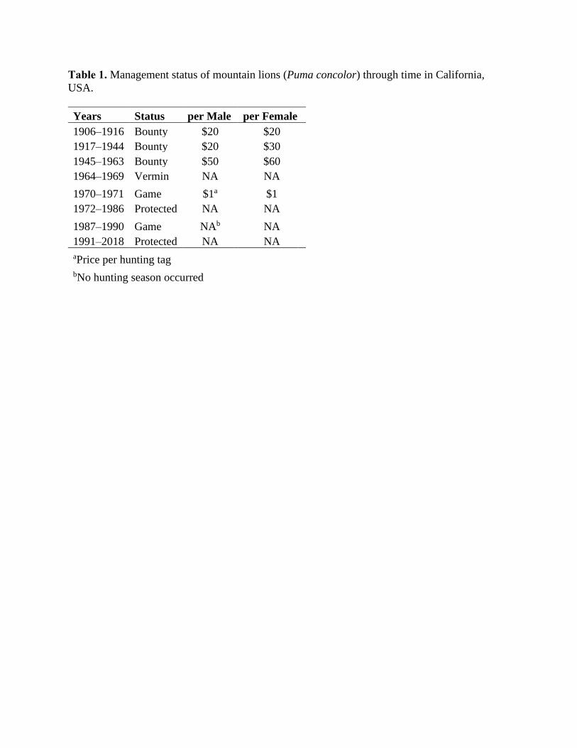
Table 1. Management status of mountain lions (Puma concolor) through time in California,
USA.
Years Status per Male per Female
1906–1916 Bounty $20 $20
1917–1944 Bounty $20 $30
1945–1963 Bounty $50 $60
1964–1969 Vermin NA NA
1970–1971 Game $1a $1
1972–1986 Protected NA NA
1987–1990 Game NAb NA
1991–2018 Protected NA NA
aPrice per hunting tag
bNo hunting season occurred
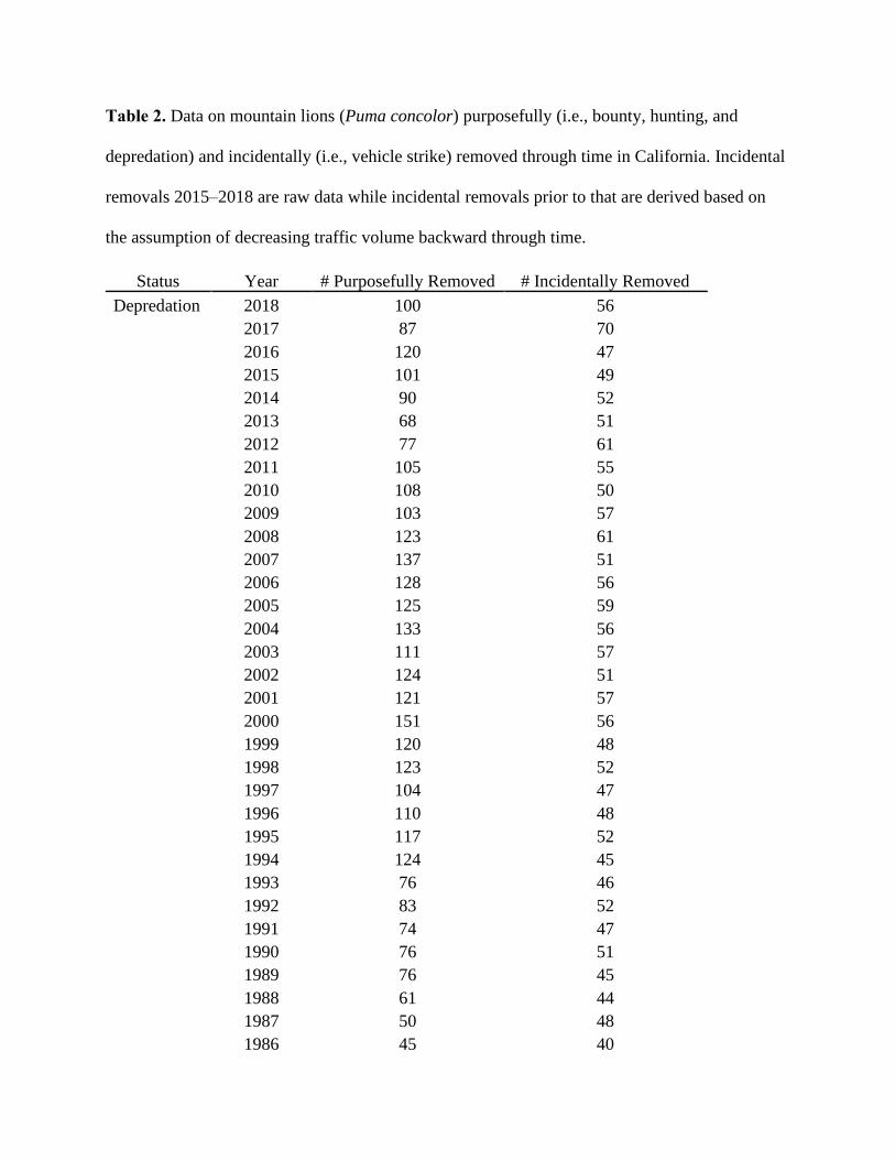
Table 2. Data on mountain lions (Puma concolor) purposefully (i.e., bounty, hunting, and
depredation) and incidentally (i.e., vehicle strike) removed through time in California. Incidental
removals 2015–2018 are raw data while incidental removals prior to that are derived based on
the assumption of decreasing traffic volume backward through time.
Status Year # Purposefully Removed # Incidentally Removed
Depredation 2018 100 56
2017 87 70
2016 120 47
2015 101 49
2014 90 52
2013 68 51
2012 77 61
2011 105 55
2010 108 50
2009 103 57
2008 123 61
2007 137 51
2006 128 56
2005 125 59
2004 133 56
2003 111 57
2002 124 51
2001 121 57
2000 151 56
1999 120 48
1998 123 52
1997 104 47
1996 110 48
1995 117 52
1994 124 45
1993 76 46
1992 83 52
1991 74 47
1990 76 51
1989 76 45
1988 61 44
1987 50 48
1986 45 40

Status Year # Purposefully Removed # Incidentally Removed
1985 58 47
1984 37 44
1983 26 42
1982 18 48
1981 12 46
1980 12 48
1979 21 40
1978 8 36
1977 7 36
1976 6 44
1975 2 44
1974 3 37
1973 4 40
1972 6 42
Hunting 1971 35 41
1970 83 36
Bounty 1963 99 33
1962 115 38
1961 144 36
1960 127 39
1959 112 37
1958 136 35
1957 157 39
1956 165 33
1955 188 34
1954 155 36
1953 188 35
1952 167 31
1951 140 33
1950 202 35
1949 228 29
1948 188 35
1947 199 35
1946 213 34
1945 152 34
1944 177 29
1943 155 29
1942 159 30
1941 236 29

Status Year # Purposefully Removed # Incidentally Removed
1940 224 28
1939 291 28
1938 252 27
1937 221 29
1936 185 31
1935 249 27
1934 225 32
1933 268 23
1932 313 27
1931 292 26
1930 293 24
1929 297 23
1928 339 26
1927 247 24
1926 253 26
1925 240 27
1924 279 28
1923 230 23
1922 302 21
1921 252 25
1920 238 22
1919 263 22
1918 192 23
1917 171 24
1916 181 25
1915 170 23
1914 196 23
1913 232 22
1912 253 21
1911 270 21
1910 322 20
1909 360 22
1908 443 20
1907 117 23
1906 118 23

Table 3. Demonstration of systematically adjusted density values for each habitat suitability
class and derived range of initial mountain lion population values for back calculation of
mountain lion (Puma concolor) population projections.
Suitability
Habitat Suitability
Scorea Size
Mountain Lion Density
(animals/100km2)b
High >0.60 170,486 km2 2.20
Medium 0.41–0.60 63,085 km2 1.60
Low 0.20–0.40 24,641 km2 1.00
None <0.20 165,759 km2 0.00
aHabitat suitability thresholds were on a scale of 0–1
bDensities of mountain lions (animals/100km2) for each habitat suitability.

Table 4. Statistical comparisons of slopes of simulated population trends over 10-year periods
for the lower and upper 10% starting population values, respectively, using a Student’s t-test.
The first mean lower 10% value represents the mean of the lowest 10% of the simulated
population estimates for the first year in the comparison. For example, the value 2,898 represents
the mean value of the lower 10% of simulated population estimates for 1910, while the value
3,094 represents the mean value of the lower 10% of simulated population estimates for 1920.
The same associations apply for the upper 10% column.
Years compared Mean lower 10% Mean upper 10% t-scorea p-value
1910 & 1920 2,898; 3,094 3,816; 3,996 -0.34 0.74
1920 & 1930 3,094; 2,749 3,996; 3,527 -1.69 0.09
1930 & 1940 2,749; 2,139 3,527; 2,749 1.48 0.14
1940 & 1950 2,139; 1,729 2,749; 2,210 1.64 0.10
1950 & 1960 1,729; 1,177 2,210; 1,549 1.11 0.27
1960 & 1970 1,177; 927 1,549; 1,364 -1.68 0.09
1970 & 1980 927; 1,389 1,364; 1,984 -176 0.08
1980 & 1990 1,389; 1,840 1,984; 2,676 -2.48 0.01
1990 & 2000 1,840; 1,897 2,676; 3,103 -6.15 <0.01
2000 & 2010 1,897; 1,524 3,103; 3,685 -10.75 <0.01
aDegrees of Freedom = 3,996

SUPPLEMENTARY MATERIAL
We estimated the sensitivity of population simulations to changes in annual population
growth (λ) and additional annual mortality (m) rates. We allowed the input value to vary in a
uniform distribution between 500 and 5,000 while changing the mean λ and m values. We set the
mean value of λ variously at 1.11, 1.14 (used in main analyses), and 1.17, and that of m at 0.08,
0.10 (used in the main analyses), and 0.12. We conducted 1,000 simulations for each λ and m
value, which resulted in 9 different groupings of 1,000 simulations. For example, one set of
1,000 simulations had a mean λ value of 1.11 and a mean m value of 0.08. Visual examination of
the results demonstrated that changes to mean λ and m values, respectively, did change the
results of our population simulations, but the population trends (i.e., overall decreasing during
the bounty period and overall increasing post-bounty) were unchanged (Supplementary Figure
1).
We also estimated the sensitivity of our simulations to input population values. We used
the parameterizations described in the manuscript but held the input value constant for 1,000
simulations. We did this for different input population values in intervals of 500. For example,
we conducted 1,000 simulations wherein we held the input population value constant at 500. We
then conducted another 1,000 simulations wherein we held the input population constant at
1,000. We did this at intervals of 500 up to a starting population value of 5,000. Visual
examination of the results demonstrated that influence of starting value on simulated population
trends decreased around the year 2000 (Supplementary Figure 2). Furthermore, starting
population value did not change the overall trends of simulated populations during the bounty
(i.e., decreasing mountain lion population size) or post-bounty up to the mid-1990s (i.e.,
increasing mountain lion population size).
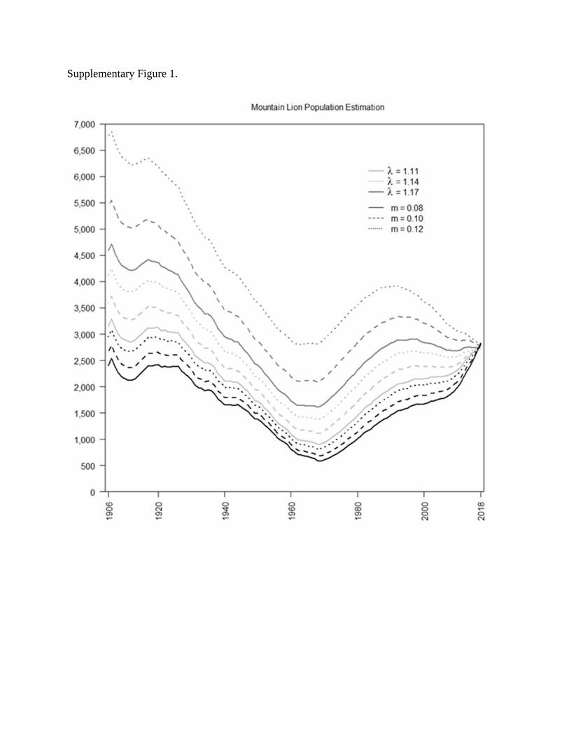
Supplementary Figure 1.

Supplementary Figure 2.