Embed Size (px)
Citation preview

A Red Ryder Christmas
\
A Bean Counter’s Journey Through
The World of Seasonal Barometers
Wayne Whaley
Witter & Lester, Inc.
February 28, 2013

Table of Contents
Page
1. Abstract ….….…..……………………………………………………………………… i-vi
2. The January Barometer…….…………………………………………………….. 1
3. The Month to Year Directional Comparison…….……………………… 2
4. The Month to Year Normalized Hit or Miss Comparison….……… 4
5. The Month to Year Correlation Coefficient Comparison…………. 7
6. The Month to Year Correlation Study Summary …………………….. 9
7. Introducing the TOY Barometer……………………………….…………….. 10
8. Bear Market TOYs…………………………………………………………………… 14
9. The January vs TOY Barometer Comparison…………………………… 16
10. A Red Ryder Christmas…………………………………………………….…….. 18
11. Wayne’s Intermediate Time Frame Seasonal Model…………........ 20
12. The Seasonal Model’s Trading Performance ……..……………..……. 22
13. Summary…………………………..………………………………………………….... 25
Addendum 1 – The January Barometer – The Detailed Breakdown
Addendum 2 – Wayne’s Version of the ‘Sell in May and Go Away Story
Addendum 3 – The Election Cycle Story
Addendum 4 – The Wayne Whaley Story
A Red Ryder Christmas – Abstract
Owing tremendously to previous students of seasonal tendencies, such
as Yale Hirsch and Arthur Merrill, astute traders have, for several
decades, been cognizant of the intermediate implications arising from
the market’s observed disposition at the turn of each calendar year. For
the last half century, indicators such as the ‘January Barometer’, the
‘First Five Days of January’, and various ‘End of the Year’ holiday studies
have served to document these tendencies.
My initial objective was to determine if January’s predictive reputation
was statistically warranted, and if any other month could provide a
possible midyear update and/or validation of any insight imparted upon
the markets future direction by January’s behavior. This curiosity into
the nature of seasonal barometers, eventually led me to discoveries far
beyond the original intended objective of simply evaluating the
predictive abilities of each of the twelve months.
As a study benchmark, a full review of the January barometer’s track
record was documented. It was noted that January did indeed exhibit
i

statistically significant forecasting accuracy when focused on positive
Januarys, but could only manufacture coin toss odds when dealt with
negative Januarys.
The month/year comparison analysis, for each of the twelve months,
began with an evaluation of each month’s ability to forecast the direction
of the next twelve month’s S&P performance, that is, what percent of the
years did the sign of each month’s move, match the sign of the next
twelve months direction. Based on this ‘same sign’, evaluation criteria,
January was, indeed, the best 12 month forecasting tool, with a 70.97%
probability of forecasting the next year’s direction, as compared to
66.13% for April, which was finished a distant second.
Noting that this was not an extremely scientific approach, I then
embarked upon converting all the monthly and yearly moves to
normalized measures and examined each month’s ability to post a move
that fell within one standard deviation of the next twelve month’s
normalized move. Based on this evaluation approach, January and June
finished tied for first with a 62.90% probability of a successful one
standard deviation match of the next 12 months S&P move.
ii
Thirdly, I thought it prudent to calculate the Pearson Correlation
Coefficient (-1 to +1) between each of the twelve months and their
corresponding following year. Again, the month of January finished first
(+0.246) in this correlation measurement followed by April (+0.166). I
concluded, if you were forced to hitch your wagon to one of the 12
calendar months, January was the horse to follow. However,
disappointed that none of the 12 months produced more reliable
correlation statistics than were observed in this study, I pondered if
better seasonal barometers were not available.
In an effort to resolve, which time period of the year was the King Pin of
seasonal barometers, I implored my computer to exhaustively scan S&P
performance over every time period of the year and determine which
time frame’s behavior was proprietor of the highest correlation
measures, relative to the following year’s performance. This involved an
analysis of 30,295 different time frames throughout the year, ranging
from 7 to 90 days.
I found that if one does not constrain his seasonal barometer selection
solely to the twelve calendar months, the time period from November
iii
19 through January 19 has a superior 12 month forecasting record than
both the traditional January Barometer, and any other 7 to 90 day time
period you care to consider. This time period, which I have labeled the
TOY (Turn of Year) Barometer, accurately predicted the next year’s
market direction in 80.65% of the post 1949 database cases as
compared to 70.97% for the month of January, with a measurably higher
correlation coefficient (+0.39). Thirty one of the thirty two +3% TOYs
were followed by positive years and nine of the 13 negative TOYs were
followed by negative years, with 11 of those 13 negative TOY periods
experiencing at least a 12.5% Drawdown at some point over the
following 12 months.
In a very special Red Ryder TOY setup case; if a negative TOY Year
(January 19 – January 19), concludes with a positive TOY period
(November 19 – January 19), the following TOY year has been up at least
10% in all ten occasions this setup has developed with a remarkable ten
signal average/median annual return of 27.25/28.71%, catching five of
the six +30% years over this post 1949 sample set.
iv
Unfortunately, I was not able to identify any mid-year periods which
provided comparable forecasting accuracy to that identified by several
periods residing between November and February.
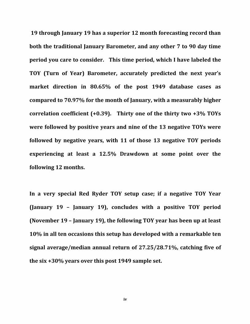
I combined the Toy Barometer and Red Ryder Signals with my versions
of two traditional seasonal stalwarts, the ‘Sell In May and Go Away’
thesis, and the Election Cycle Phenomenon, to produce the following five
signal rating results.
SEASONAL MODEL PERFORMANCE SEASONAL NUMBER AVERAGE RATING OF YEARS ANNUAL%CHG -1 6.29 -19.85 0 11.62 2.98
1 15.58 7.10
2 17.20 12.14
3 9.55 28.09
4 2.90 37.04
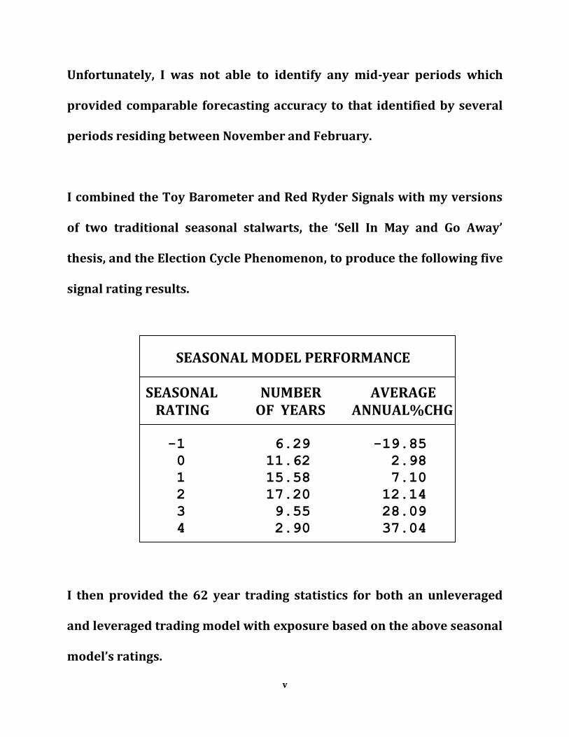
I then provided the 62 year trading statistics for both an unleveraged
and leveraged trading model with exposure based on the above seasonal
model’s ratings.
v
MARKET EXPOSURE VS SSNL RATING SEASONAL EQUITY EXPOSURE
RATING UNLEVERAGED LEVERAGED -1 0.00 -0.50
0 0.25 0.00
1 0.50 0.50
2 0.75 1.00
3 1.00 1.50
4 1.00 2.00
EXPOSURE MODEL STATISTICS COMPARISON B&H UNLEV- LEVER- STATISTIC S&P ERAGED ERAGED PCT OF UP YEARS = 73.02 87.30 90.48
AVG YRLY % CHG = 8.71 11.09 16.49
MAX DRAWDOWN = -56.78 -26.34 -35.12
AVG DAILY VOLAT = 0.659 0.358 0.492
BETA TO S&P = 1.00 0.543 0.747
RISK ADJ ALPHA = 0.00 11.69 13.38
B&H = Buy & Hold
A well researched exposure model should arguably consist of some mix
of seasonal, tape, interest rate influences, sentiment, economic and
valuation systems. The intermediate seasonal model, which I have
introduced, is an excellent foundation for such an endeavor.
vi


The January Barometer
The table below shows the S&P performance for the post 1949 time
period as a function of three different levels of January performance.
FORWARD S&P PERFORMANCE VS JANUARY PERFORMANCE
CATEGORY WEEK MONTH QTR 6MTS 12MTS
AFTER A #UP-DN = 13- 5 12- 6 17- 1 17- 1 17- 1
+4% AVG%CHG= 0.65 1.01 4.69 9.38 15.44
JANUARY MED%CHG= 0.78 0.62 4.78 7.32 13.82
AFTER A #UP-DN = 13- 7 12- 8 15- 5 14- 6 16- 4
0 TO 4% AVG%CHG= 0.41 0.30 2.87 3.91 10.21
JANUARY MED%CHG= 0.79 0.52 2.96 2.73 10.70
AFTER A #UP-DN = 13-11 9-15 13-11 12-12 13-11
NEGATIVE AVG%CHG= -0.19 -1.36 0.49 -0.76 1.25
JANUARY MED%CHG= 0.50 -1.92 0.52 0.44 3.28
HIST AVG= 0.17 0.72 2.17 4.36 8.69
The detailed annual performance breakdown for the January Barometer
is included in Addendum 1. The primary criticism of the January
Barometer is that it doesn’t provide a lot of guidance for Bearish setups
as the annual performance after a negative January is close to a coin toss.
Let us begin our journey of alternatives with an examination of January
stacks up against the remaining eleven calendar months in terms of 12
month forecasting ability.
1
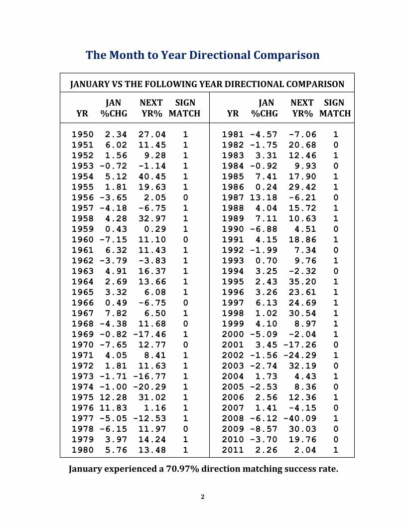
The Month to Year Directional Comparison
JANUARY VS THE FOLLOWING YEAR DIRECTIONAL COMPARISON
JAN NEXT SIGN JAN NEXT SIGN YR %CHG YR% MATCH YR %CHG YR% MATCH
1950 2.34 27.04 1 1981 -4.57 -7.06 1
1951 6.02 11.45 1 1982 -1.75 20.68 0
1952 1.56 9.28 1 1983 3.31 12.46 1
1953 -0.72 -1.14 1 1984 -0.92 9.93 0
1954 5.12 40.45 1 1985 7.41 17.90 1
1955 1.81 19.63 1 1986 0.24 29.42 1
1956 -3.65 2.05 0 1987 13.18 -6.21 0
1957 -4.18 -6.75 1 1988 4.04 15.72 1
1958 4.28 32.97 1 1989 7.11 10.63 1
1959 0.43 0.29 1 1990 -6.88 4.51 0
1960 -7.15 11.10 0 1991 4.15 18.86 1
1961 6.32 11.43 1 1992 -1.99 7.34 0
1962 -3.79 -3.83 1 1993 0.70 9.76 1
1963 4.91 16.37 1 1994 3.25 -2.32 0
1964 2.69 13.66 1 1995 2.43 35.20 1
1965 3.32 6.08 1 1996 3.26 23.61 1
1966 0.49 -6.75 0 1997 6.13 24.69 1
1967 7.82 6.50 1 1998 1.02 30.54 1
1968 -4.38 11.68 0 1999 4.10 8.97 1
1969 -0.82 -17.46 1 2000 -5.09 -2.04 1
1970 -7.65 12.77 0 2001 3.45 -17.26 0
1971 4.05 8.41 1 2002 -1.56 -24.29 1
1972 1.81 11.63 1 2003 -2.74 32.19 0
1973 -1.71 -16.77 1 2004 1.73 4.43 1
1974 -1.00 -20.29 1 2005 -2.53 8.36 0
1975 12.28 31.02 1 2006 2.56 12.36 1
1976 11.83 1.16 1 2007 1.41 -4.15 0
1977 -5.05 -12.53 1 2008 -6.12 -40.09 1
1978 -6.15 11.97 0 2009 -8.57 30.03 0
1979 3.97 14.24 1 2010 -3.70 19.76 0
1980 5.76 13.48 1 2011 2.26 2.04 1
January experienced a 70.97% direction matching success rate.
2
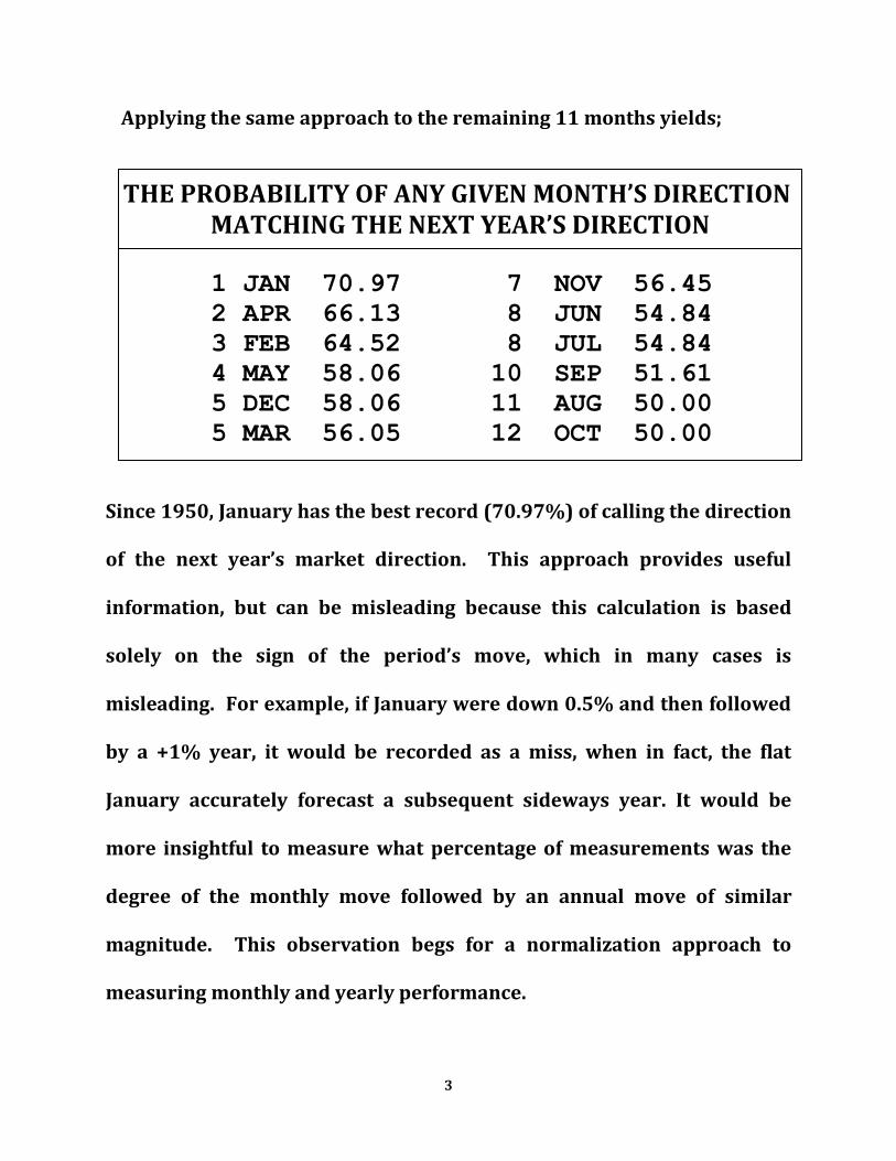
Applying the same approach to the remaining 11 months yields;
THE PROBABILITY OF ANY GIVEN MONTH’S DIRECTION MATCHING THE NEXT YEAR’S DIRECTION
1 JAN 70.97 7 NOV 56.45
2 APR 66.13 8 JUN 54.84
3 FEB 64.52 8 JUL 54.84
4 MAY 58.06 10 SEP 51.61
5 DEC 58.06 11 AUG 50.00
5 MAR 56.05 12 OCT 50.00
Since 1950, January has the best record (70.97%) of calling the direction
of the next year’s market direction. This approach provides useful
information, but can be misleading because this calculation is based
solely on the sign of the period’s move, which in many cases is
misleading. For example, if January were down 0.5% and then followed
by a +1% year, it would be recorded as a miss, when in fact, the flat
January accurately forecast a subsequent sideways year. It would be
more insightful to measure what percentage of measurements was the
degree of the monthly move followed by an annual move of similar
magnitude. This observation begs for a normalization approach to
measuring monthly and yearly performance.
3
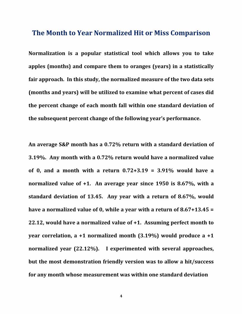
The Month to Year Normalized Hit or Miss Comparison
Normalization is a popular statistical tool which allows you to take
apples (months) and compare them to oranges (years) in a statistically
fair approach. In this study, the normalized measure of the two data sets
(months and years) will be utilized to examine what percent of cases did
the percent change of each month fall within one standard deviation of
the subsequent percent change of the following year’s performance.
An average S&P month has a 0.72% return with a standard deviation of
3.19%. Any month with a 0.72% return would have a normalized value
of 0, and a month with a return 0.72+3.19 = 3.91% would have a
normalized value of +1. An average year since 1950 is 8.67%, with a
standard deviation of 13.45. Any year with a return of 8.67%, would
have a normalized value of 0, while a year with a return of 8.67+13.45 =
22.12, would have a normalized value of +1. Assuming perfect month to
year correlation, a +1 normalized month (3.19%) would produce a +1
normalized year (22.12%). I experimented with several approaches,
but the most demonstration friendly version was to allow a hit/success
for any month whose measurement was within one standard deviation
4
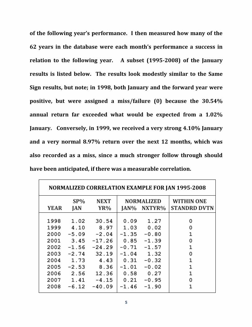
of the following year’s performance. I then measured how many of the
62 years in the database were each month’s performance a success in
relation to the following year. A subset (1995-2008) of the January
results is listed below. The results look modestly similar to the Same
Sign results, but note; in 1998, both January and the forward year were
positive, but were assigned a miss/failure (0) because the 30.54%
annual return far exceeded what would be expected from a 1.02%
January. Conversely, in 1999, we received a very strong 4.10% January
and a very normal 8.97% return over the next 12 months, which was
also recorded as a miss, since a much stronger follow through should
have been anticipated, if there was a measurable correlation.
NORMALIZED CORRELATION EXAMPLE FOR JAN 1995-2008 SP% NEXT NORMALIZED WITHIN ONE YEAR JAN YR% JAN% NXTYR% STANDRD DVTN 1998 1.02 30.54 0.09 1.27 0 1999 4.10 8.97 1.03 0.02 0 2000 -5.09 -2.04 -1.35 -0.80 1 2001 3.45 -17.26 0.85 -1.39 0 2002 -1.56 -24.29 -0.71 -1.57 1 2003 -2.74 32.19 -1.04 1.32 0 2004 1.73 4.43 0.31 -0.32 1 2005 -2.53 8.36 -1.01 -0.02 1 2006 2.56 12.36 0.58 0.27 1 2007 1.41 -4.15 0.21 -0.95 0 2008 -6.12 -40.09 -1.46 -1.90 1
5
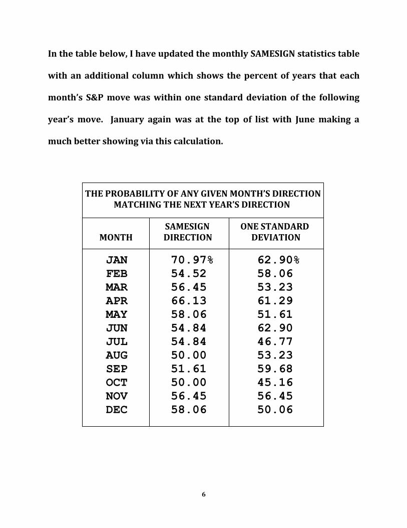
In the table below, I have updated the monthly SAMESIGN statistics table
with an additional column which shows the percent of years that each
month’s S&P move was within one standard deviation of the following
year’s move. January again was at the top of list with June making a
much better showing via this calculation.
THE PROBABILITY OF ANY GIVEN MONTH’S DIRECTION MATCHING THE NEXT YEAR’S DIRECTION SAMESIGN ONE STANDARD MONTH DIRECTION DEVIATION
JAN 70.97% 62.90% FEB 54.52 58.06 MAR 56.45 53.23 APR 66.13 61.29 MAY 58.06 51.61 JUN 54.84 62.90 JUL 54.84 46.77 AUG 50.00 53.23 SEP 51.61 59.68 OCT 50.00 45.16 NOV 56.45 56.45 DEC 58.06 50.06
6

The Month to Year Correlation Coefficient Comparison
A third measure of interest is each of the twelve month’s correlation
coefficient to the following year’s performance. Recall from Statistics
101, that a correlation coefficient represents the quality of the linear
relation between two sets of data. A value of +1 represents a perfect fit,
while a value of -1 represents a perfect negative correlation. If there is
no correlation, the coefficient should hover close to zero. If there was a
strong correlation between a particular month’s performance and the
following year’s move, we would expect to see the correlation coefficient
gravitate toward a value of +1.
Since I desire that you stick around for the rest of the movie, I will pass
on the temptation to use the unused bottom half of this page to provide
you with the mathematical equation used to calculate the Pearson
Correlation Coefficient. You know how to google, and besides most
modern day graphing calculators will provide the correlation coefficient
between any two sets of data.
7

Utilizing the Pearson Correlation Coefficient equation, January and April
again come in first and second although, admittedly, reflecting much less
correlation than most barometer enthusiast would care to acknowledge.
I have added a third column to our previous table of correlation results
with each month’s Pearson Correlation Coefficient added. The AVERAGE
column is the average of the three correlation measures in the first three
columns. You may have noticed that averaging the three measurements
required converting the standard Pearson Correlation Coefficient
measure from ‘–1 to +1’ to ‘0 to 100’. Green = First, Blue = Second
SUMMARY OF MONTH TO YEAR CORRELATION MEASURES MT SAMESIGN NORMALIZED PEARSONCC AVERAGE RANK
JAN 70.97 62.90 0.246 65.39 1
FEB 64.52 58.06 0.078 58.83 3
MAR 56.45 53.23 -.133 51.01 9
APR 66.13 61.29 0.166 61.85 2
MAY 58.06 51.61 -.003 53.17 6
JUN 54.84 62.90 0.062 56.94 4
JUL 54.84 46.77 -.013 50.32 10
AUG 50.00 53.23 -.144 49.18 12
SEP 51.61 59.68 -.059 52.78 7
OCT 50.00 45.16 0.062 49.43 11
NOV 56.45 56.45 0.119 56.28 5
DEC 58.06 50.00 -0.041 52.00 8
8
Month to Year Correlation Study Summary
Based on the above analysis, there is substantial evidence supporting
the explanation for January’s popularity as the calendar month
Barometer of choice, as it ranked first in each of the three measures we
have examined.
I was disappointed to discover that none of the twelve calendar months
carried more than a 0.21% correlation coefficient vs the corresponding
12 month move, nor was able to predict the direction of the following
year with more than 70% accuracy.
This desire for higher accuracy brings us to the crux of this seasonal
analysis study. Could we find a better barometer, if we were not
constrained to calendar ‘month’ analysis? For example, what about
midmonth periods such as December 15 through January 15? And if we
are going to burden the computer with the task of scanning all 365
potential months in a year, why not take an extra second and search for
all time periods of all time lengths?
9
Introducing the TOY Barometer
I set up a scan to look at every time period in the 365 day calendar, in
time intervals of from seven to 90 days (week to quarter). This resulted
in a scan of 30,295 different time periods in an effort to determine which
one had the best record of forecasting the nature of the next twelve
months move. I chose as my measure of effectiveness (MOE), the
average of the Samesign, Normalized Hits, and Pearson Correlation
Coefficient approaches, which I have introduced above. The time period,
which this exercise determined to have the highest correlation to the
following year, was the two month period from November 19 to January
19. Since this two month time period (Nov19-Jan19) extends across the
Turn of the Year (TOY) and encompasses the gift giving season, I have
coined it the ‘TOY Barometer’. Below is a comparison of the one year
forecasting record of the month of January versus the TOY period via the
three correlation measures, I have previously introduced. The TOY
Barometer showed improvement in all three measurements and
accurately forecast the direction of the following year’s S&P move in
80.65% of the 62 years evaluated from 1950 through 2011, a marked
improvement over the January Barometer’s 71% success rate.
10
THE JANUARY AND TOY BAROMETER COMPARISON BAROMETER SAMESIGN NORMALIZED PEARSONCC AVERAGE
JANUARY 70.97 62.90 0.246 65.39
TOY 80.65 67.74 0.391 72.65
The TOY Barometer’s predictive ability benefits from the fact it’s setup
period includes several subset time frames which have, in their own
right, shown predictive capability; such as the Thanksgiving Holiday
week, the Christmas Holiday week, the last week of the year and the first
week of the year. Also, many an investment methodology involves turn
of the year contributions which may tip the market’s hand as to levels of
money flow which may potentially ensue over the course of the year and
contribute to both the TOY and January Barometer’s successful track
record.
11
Since 1950, the S&P has finished positive in the following TOY year
(Jan19-Jan19) in 31 of those 32 years in which TOY performance
(Nov19-Jan19) exceeded 3%. In the 1987 exception, the S&P was up
24% from January 19 through August 13, before succumbing to an
assault on double digit interest rates during the fall of that, the year of
our beloved Black Monday. The 32 previous +3% TOY cases are listed
below.
ONE YEAR (JAN19-JAN19) S&P PERFORMANCE AFTER A +3% TOY
# YEAR TOY% NEXTYR% # YEAR TOY% NEXTYR% 1 1950 4.26 27.89 17 1980 6.56 20.98
2 1951 7.55 13.08 18 1983 6.02 14.99
3 1952 6.69 10.17 19 1985 5.50 21.66
4 1954 5.25 44.51 20 1986 4.91 29.22
5 1955 4.51 33.36 21 1987 13.33 -7.43
6 1958 3.24 35.79 22 1988 3.86 15.08
7 1959 4.66 8.78 23 1989 7.67 18.21
8 1961 7.08 21.72 24 1991 4.04 26.08
9 1963 8.96 17.67 25 1992 10.39 3.88
10 1964 6.48 12.98 26 1997 4.58 23.88
11 1967 5.61 13.75 27 1999 8.53 16.39
12 1971 13.09 12.16 28 2004 9.34 3.93
13 1972 13.39 15.56 29 2009 5.40 35.30
14 1975 4.05 38.56 30 2010 5.05 11.45
15 1976 9.27 5.62 31 2011 6.85 2.54
16 1979 5.64 11.35 32 2012 8.13 13.05
33 2013 7.19 ?
NEXT YEAR #UP-DN= 31-1 AVG%CHG=16.67 MED%CHG=15.01
12
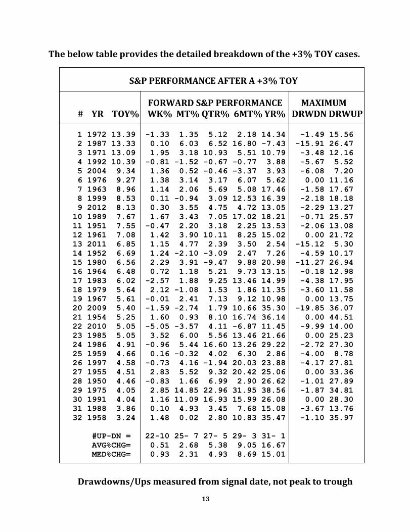
The below table provides the detailed breakdown of the +3% TOY cases.
S&P PERFORMANCE AFTER A +3% TOY FORWARD S&P PERFORMANCE MAXIMUM # YR TOY% WK% MT% QTR% 6MT% YR% DRWDN DRWUP
1 1972 13.39 -1.33 1.35 5.12 2.18 14.34 -1.49 15.56
2 1987 13.33 0.10 6.03 6.52 16.80 -7.43 -15.91 26.47
3 1971 13.09 1.95 3.18 10.93 5.51 10.79 -3.48 12.16
4 1992 10.39 -0.81 -1.52 -0.67 -0.77 3.88 -5.67 5.52
5 2004 9.34 1.36 0.52 -0.46 -3.37 3.93 -6.08 7.20
6 1976 9.27 1.38 3.14 3.17 6.07 5.62 0.00 11.16
7 1963 8.96 1.14 2.06 5.69 5.08 17.46 -1.58 17.67
8 1999 8.53 0.11 -0.94 3.09 12.53 16.39 -2.18 18.18
9 2012 8.13 0.30 3.55 4.75 4.72 13.05 -2.29 13.27
10 1989 7.67 1.67 3.43 7.05 17.02 18.21 -0.71 25.57
11 1951 7.55 -0.47 2.20 3.18 2.25 13.53 -2.06 13.08
12 1961 7.08 1.42 3.90 10.11 8.25 15.02 0.00 21.72
13 2011 6.85 1.15 4.77 2.39 3.50 2.54 -15.12 5.30
14 1952 6.69 1.24 -2.10 -3.09 2.47 7.26 -4.59 10.17
15 1980 6.56 2.29 3.91 -9.47 9.88 20.98 -11.27 26.94
16 1964 6.48 0.72 1.18 5.21 9.73 13.15 -0.18 12.98
17 1983 6.02 -2.57 1.88 9.25 13.46 14.99 -4.38 17.95
18 1979 5.64 2.12 -1.08 1.53 1.86 11.35 -3.60 11.58
19 1967 5.61 -0.01 2.41 7.13 9.12 10.98 0.00 13.75
20 2009 5.40 -1.59 -2.74 1.79 10.66 35.30 -19.85 36.07
21 1954 5.25 1.60 0.93 8.10 16.74 36.14 0.00 44.51
22 2010 5.05 -5.05 -3.57 4.11 -6.87 11.45 -9.99 14.00
23 1985 5.05 3.52 6.00 5.56 13.46 21.66 0.00 25.23
24 1986 4.91 -0.96 5.44 16.60 13.26 29.22 -2.72 27.30
25 1959 4.66 0.16 -0.32 4.02 6.30 2.86 -4.00 8.78
26 1997 4.58 -0.73 4.16 -1.94 20.03 23.88 -4.17 27.81
27 1955 4.51 2.83 5.52 9.32 20.42 25.06 0.00 33.36
28 1950 4.46 -0.83 1.66 6.99 2.90 26.62 -1.01 27.89
29 1975 4.05 2.85 14.85 22.96 31.95 38.56 -1.87 34.81
30 1991 4.04 1.16 11.09 16.93 15.99 26.08 0.00 28.30
31 1988 3.86 0.10 4.93 3.45 7.68 15.08 -3.67 13.76
32 1958 3.24 1.48 0.02 2.80 10.83 35.47 -1.10 35.97
#UP-DN = 22-10 25- 7 27- 5 29- 3 31- 1
AVG%CHG= 0.51 2.68 5.38 9.05 16.67
MED%CHG= 0.93 2.31 4.93 8.69 15.01
Drawdowns/Ups measured from signal date, not peak to trough
13
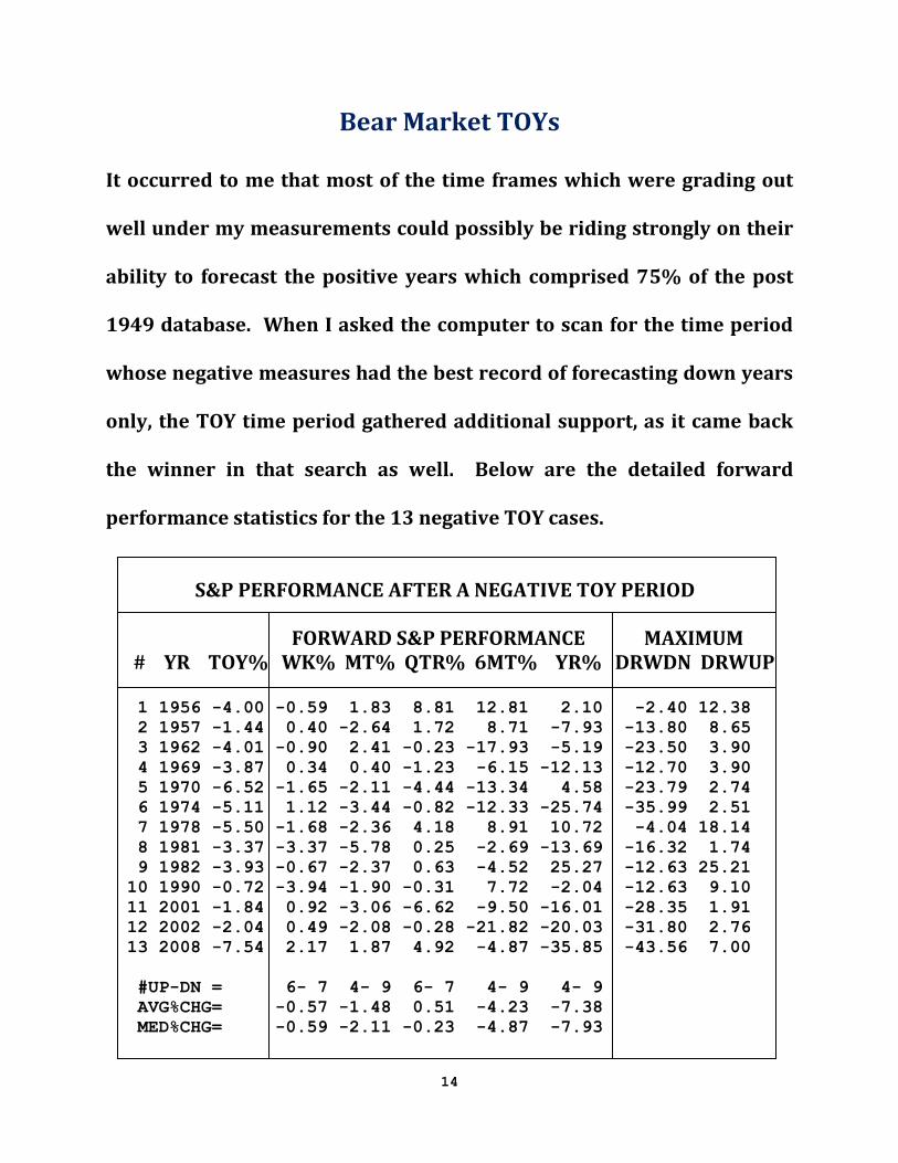
Bear Market TOYs
It occurred to me that most of the time frames which were grading out
well under my measurements could possibly be riding strongly on their
ability to forecast the positive years which comprised 75% of the post
1949 database. When I asked the computer to scan for the time period
whose negative measures had the best record of forecasting down years
only, the TOY time period gathered additional support, as it came back
the winner in that search as well. Below are the detailed forward
performance statistics for the 13 negative TOY cases.
S&P PERFORMANCE AFTER A NEGATIVE TOY PERIOD FORWARD S&P PERFORMANCE MAXIMUM # YR TOY% WK% MT% QTR% 6MT% YR% DRWDN DRWUP 1 1956 -4.00 -0.59 1.83 8.81 12.81 2.10 -2.40 12.38
2 1957 -1.44 0.40 -2.64 1.72 8.71 -7.93 -13.80 8.65
3 1962 -4.01 -0.90 2.41 -0.23 -17.93 -5.19 -23.50 3.90
4 1969 -3.87 0.34 0.40 -1.23 -6.15 -12.13 -12.70 3.90
5 1970 -6.52 -1.65 -2.11 -4.44 -13.34 4.58 -23.79 2.74
6 1974 -5.11 1.12 -3.44 -0.82 -12.33 -25.74 -35.99 2.51
7 1978 -5.50 -1.68 -2.36 4.18 8.91 10.72 -4.04 18.14
8 1981 -3.37 -3.37 -5.78 0.25 -2.69 -13.69 -16.32 1.74
9 1982 -3.93 -0.67 -2.37 0.63 -4.52 25.27 -12.63 25.21
10 1990 -0.72 -3.94 -1.90 -0.31 7.72 -2.04 -12.63 9.10
11 2001 -1.84 0.92 -3.06 -6.62 -9.50 -16.01 -28.35 1.91
12 2002 -2.04 0.49 -2.08 -0.28 -21.82 -20.03 -31.80 2.76
13 2008 -7.54 2.17 1.87 4.92 -4.87 -35.85 -43.56 7.00
#UP-DN = 6- 7 4- 9 6- 7 4- 9 4- 9
AVG%CHG= -0.57 -1.48 0.51 -4.23 -7.38
MED%CHG= -0.59 -2.11 -0.23 -4.87 -7.93
14
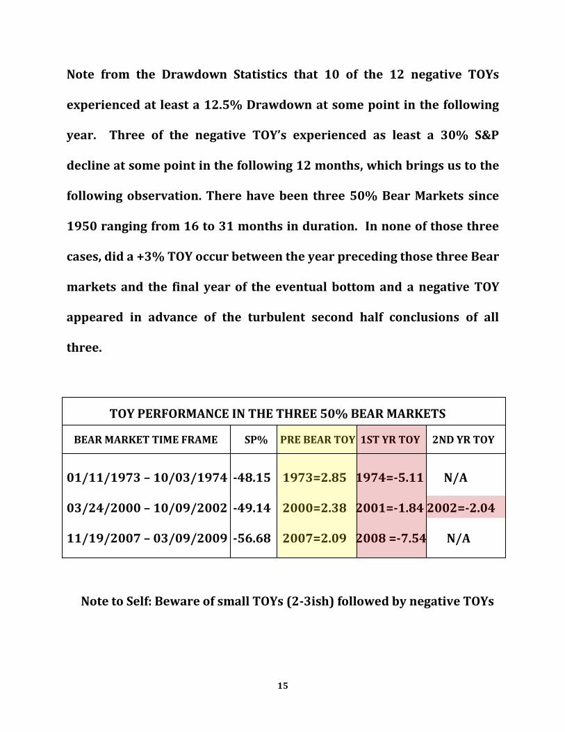
Note from the Drawdown Statistics that 10 of the 12 negative TOYs
experienced at least a 12.5% Drawdown at some point in the following
year. Three of the negative TOY’s experienced as least a 30% S&P
decline at some point in the following 12 months, which brings us to the
following observation. There have been three 50% Bear Markets since
1950 ranging from 16 to 31 months in duration. In none of those three
cases, did a +3% TOY occur between the year preceding those three Bear
markets and the final year of the eventual bottom and a negative TOY
appeared in advance of the turbulent second half conclusions of all
three.
TOY PERFORMANCE IN THE THREE 50% BEAR MARKETS BEAR MARKET TIME FRAME SP% PRE BEAR TOY 1ST YR TOY 2ND YR TOY
01/11/1973 – 10/03/1974 -48.15 1973=2.85 1974=-5.11 N/A 03/24/2000 – 10/09/2002 -49.14 2000=2.38 2001=-1.84 2002=-2.04 11/19/2007 – 03/09/2009 -56.68 2007=2.09 2008 =-7.54 N/A
Note to Self: Beware of small TOYs (2-3ish) followed by negative TOYs
15
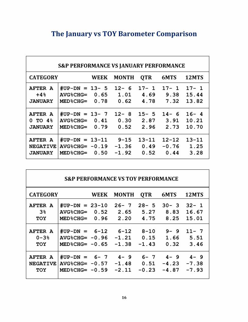
The January vs TOY Barometer Comparison
S&P PERFORMANCE VS JANUARY PERFORMANCE
CATEGORY WEEK MONTH QTR 6MTS 12MTS
AFTER A #UP-DN = 13- 5 12- 6 17- 1 17- 1 17- 1
+4% AVG%CHG= 0.65 1.01 4.69 9.38 15.44
JANUARY MED%CHG= 0.78 0.62 4.78 7.32 13.82
AFTER A #UP-DN = 13- 7 12- 8 15- 5 14- 6 16- 4
0 TO 4% AVG%CHG= 0.41 0.30 2.87 3.91 10.21
JANUARY MED%CHG= 0.79 0.52 2.96 2.73 10.70
AFTER A #UP-DN = 13-11 9-15 13-11 12-12 13-11
NEGATIVE AVG%CHG= -0.19 -1.36 0.49 -0.76 1.25
JANUARY MED%CHG= 0.50 -1.92 0.52 0.44 3.28
S&P PERFORMANCE VS TOY PERFORMANCE
CATEGORY WEEK MONTH QTR 6MTS 12MTS
AFTER A #UP-DN = 23-10 26- 7 28- 5 30- 3 32- 1
3% AVG%CHG= 0.52 2.65 5.27 8.83 16.67
TOY MED%CHG= 0.96 2.20 4.75 8.25 15.01
AFTER A #UP-DN = 6-12 6-12 8-10 9- 9 11- 7
0-3% AVG%CHG= -0.96 -1.21 0.15 1.66 5.51
TOY MED%CHG= -0.65 -1.38 -1.43 0.32 3.46
AFTER A #UP-DN = 6- 7 4- 9 6- 7 4- 9 4- 9
NEGATIVE AVG%CHG= -0.57 -1.48 0.51 -4.23 -7.38
TOY MED%CHG= -0.59 -2.11 -0.23 -4.87 -7.93
16
The significant differences in the January and TOY Barometer are
1. The TOY Barometer’s production of 33 signals in the superior
(90% accurate) category vs 18 for the January Barometer and,
2. TOY’s ability to give guidance in avoiding Bear Market years. The
S&P was down the following year after nine of the 13 negative
Toys. From the January 19 signal date, the S&P experienced at
least a 12.5% one year drawdown after 11 of the 13 Negative TOY
periods. The January Barometer was followed by positive years
after 13 of the 24 negative January Barometer signals.
With the conclusion of the TOY Story, this study presentation of 21st
century style seasonal barometers could appropriately come to a
conclusion. But given I have titled this paper ‘A Red Ryder Christmas’, I
feel obligated and compelled to provide you with at least one more
seasonal barometer statistic, one which I feel confident you will find a
definite stocking stuffer.
17
A Red Ryder Christmas
The holiday classic ‘The Christmas Story’ chronicles a year in the life of
Ralphie, a young eight year old boy, who is having a tough go of it. He is
struggling in school, bullied by the neighborhood boys, and subjected to
periodic soap cleansings of the mouth by his mother. But the story
concludes with Ralphie’s receipt of his childhood dream for Christmas, a
Red Ryder BB gun. The Red Ryder Christmas Signal parallels Ralphie’s
journey to Nirvana as the market must also first experience a poor year,
but conclude with the appearance of a once in a childhood Holiday setup
scenario. Define:
The TOY Period = S&P 500 Percent Change from Nov 19 to January 19
A TOY Year = S&P 500 Percent Change from Jan 19 to January 19
Note the TOY period is the last two months of the TOY year.
A Red Ryder TOY Signal occurs when a Negative TOY year (Jan19-Jan19)
concludes with a positive TOY Period (Nov19-Jan19).
18
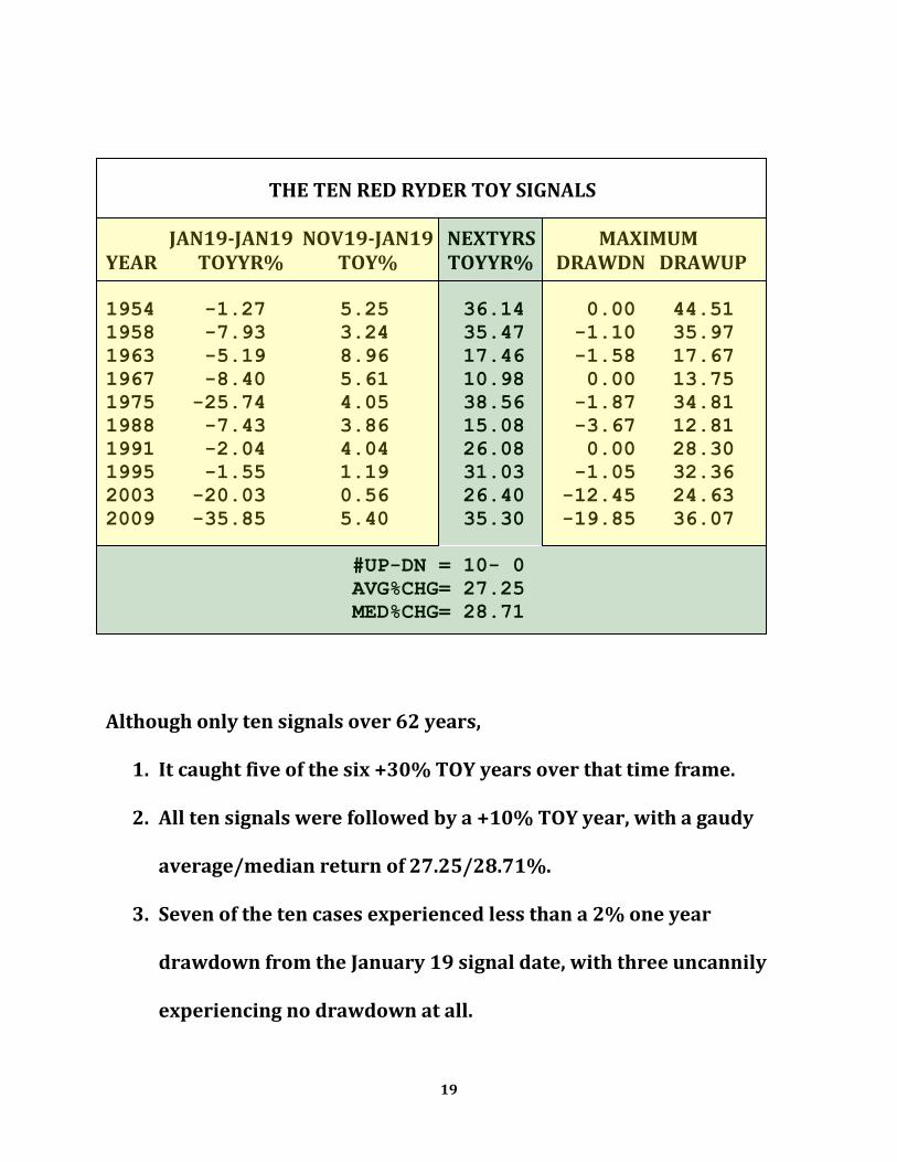
THE TEN RED RYDER TOY SIGNALS JAN19-JAN19 NOV19-JAN19 NEXTYRS MAXIMUM YEAR TOYYR% TOY% TOYYR% DRAWDN DRAWUP 1954 -1.27 5.25 36.14 0.00 44.51
1958 -7.93 3.24 35.47 -1.10 35.97
1963 -5.19 8.96 17.46 -1.58 17.67
1967 -8.40 5.61 10.98 0.00 13.75
1975 -25.74 4.05 38.56 -1.87 34.81
1988 -7.43 3.86 15.08 -3.67 12.81
1991 -2.04 4.04 26.08 0.00 28.30
1995 -1.55 1.19 31.03 -1.05 32.36
2003 -20.03 0.56 26.40 -12.45 24.63
2009 -35.85 5.40 35.30 -19.85 36.07
#UP-DN = 10- 0
AVG%CHG= 27.25
MED%CHG= 28.71
Although only ten signals over 62 years,
1. It caught five of the six +30% TOY years over that time frame.
2. All ten signals were followed by a +10% TOY year, with a gaudy
average/median return of 27.25/28.71%.
3. Seven of the ten cases experienced less than a 2% one year
drawdown from the January 19 signal date, with three uncannily
experiencing no drawdown at all.
19
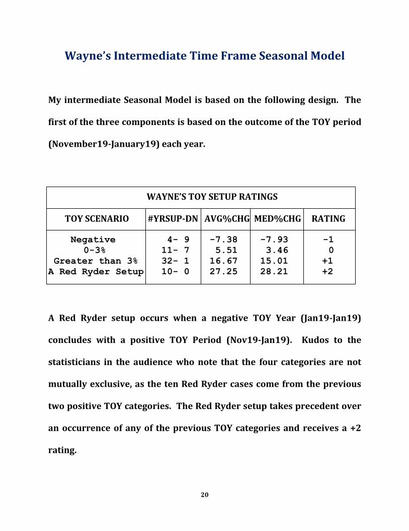
Wayne’s Intermediate Time Frame Seasonal Model
My intermediate Seasonal Model is based on the following design. The
first of the three components is based on the outcome of the TOY period
(November19-January19) each year.
WAYNE’S TOY SETUP RATINGS TOY SCENARIO #YRSUP-DN AVG%CHG MED%CHG RATING
Negative 4- 9 -7.38 -7.93 -1 0-3% 11- 7 5.51 3.46 0
Greater than 3% 32- 1 16.67 15.01 +1 A Red Ryder Setup 10- 0 27.25 28.21 +2
A Red Ryder setup occurs when a negative TOY Year (Jan19-Jan19)
concludes with a positive TOY Period (Nov19-Jan19). Kudos to the
statisticians in the audience who note that the four categories are not
mutually exclusive, as the ten Red Ryder cases come from the previous
two positive TOY categories. The Red Ryder setup takes precedent over
an occurrence of any of the previous TOY categories and receives a +2
rating.
20
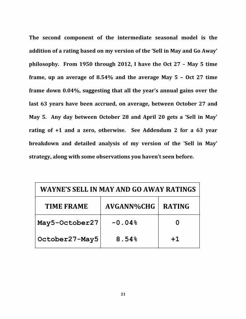
The second component of the intermediate seasonal model is the
addition of a rating based on my version of the ‘Sell in May and Go Away’
philosophy. From 1950 through 2012, I have the Oct 27 – May 5 time
frame, up an average of 8.54% and the average May 5 – Oct 27 time
frame down 0.04%, suggesting that all the year’s annual gains over the
last 63 years have been accrued, on average, between October 27 and
May 5. Any day between October 28 and April 20 gets a ‘Sell in May’
rating of +1 and a zero, otherwise. See Addendum 2 for a 63 year
breakdown and detailed analysis of my version of the ‘Sell in May’
strategy, along with some observations you haven’t seen before.
WAYNE’S SELL IN MAY AND GO AWAY RATINGS TIME FRAME AVGANN%CHG RATING May5-October27 -0.04% 0
October27-May5 8.54% +1
21
Thirdly, the average annual return in PreElection Years is 13.44% and
4.96%, in the remaining three years of the four year election cycle. The
model gives each day an Election Cycle Rating of +1, if it occurs in a
PreElection Year and a 0 otherwise. The PreElection Story details are
included in Addendum 3.
WAYNE’S ELECTION CYCLE RATINGS YEAR AVGANN%CHG RATING NonPreElection 4.96 0
PreElection 13.44 +1
Combining the ‘Sell in May’ and ‘Election Cycle’ ratings with the ‘Toy
Scenario’ ratings yields an Intermediate Seasonal Model which varies in
rating from -1 to +4 and has produced the below post 1949 annualized
S&P returns as a function of those five levels.
WAYNE’S SEASONAL MODEL PERFORMANCE SUMMARY SEASONAL NUMBER AVERAGE RATING OF YEARS ANNUAL%CHG -1 6.29 -19.85 0 11.62 2.98
1 15.58 7.10
2 17.20 12.14
3 9.55 28.09
4 2.90 37.04
22
Wayne’s Seasonal Model Trading Performance
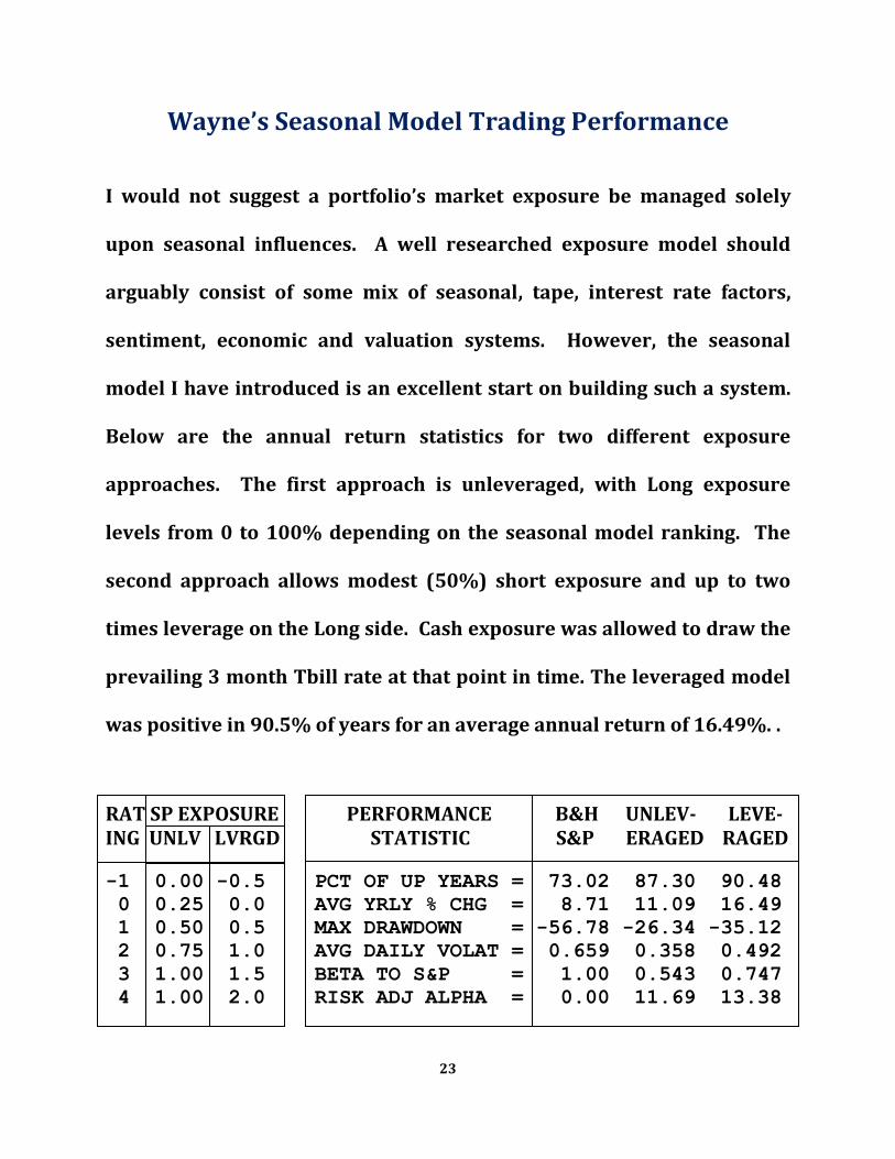
I would not suggest a portfolio’s market exposure be managed solely
upon seasonal influences. A well researched exposure model should
arguably consist of some mix of seasonal, tape, interest rate factors,
sentiment, economic and valuation systems. However, the seasonal
model I have introduced is an excellent start on building such a system.
Below are the annual return statistics for two different exposure
approaches. The first approach is unleveraged, with Long exposure
levels from 0 to 100% depending on the seasonal model ranking. The
second approach allows modest (50%) short exposure and up to two
times leverage on the Long side. Cash exposure was allowed to draw the
prevailing 3 month Tbill rate at that point in time. The leveraged model
was positive in 90.5% of years for an average annual return of 16.49%. .
RAT SP EXPOSURE PERFORMANCE B&H UNLEV- LEVE- ING UNLV LVRGD STATISTIC S&P ERAGED RAGED -1 0.00 -0.5 PCT OF UP YEARS = 73.02 87.30 90.48
0 0.25 0.0 AVG YRLY % CHG = 8.71 11.09 16.49
1 0.50 0.5 MAX DRAWDOWN = -56.78 -26.34 -35.12
2 0.75 1.0 AVG DAILY VOLAT = 0.659 0.358 0.492
3 1.00 1.5 BETA TO S&P = 1.00 0.543 0.747
4 1.00 2.0 RISK ADJ ALPHA = 0.00 11.69 13.38
23
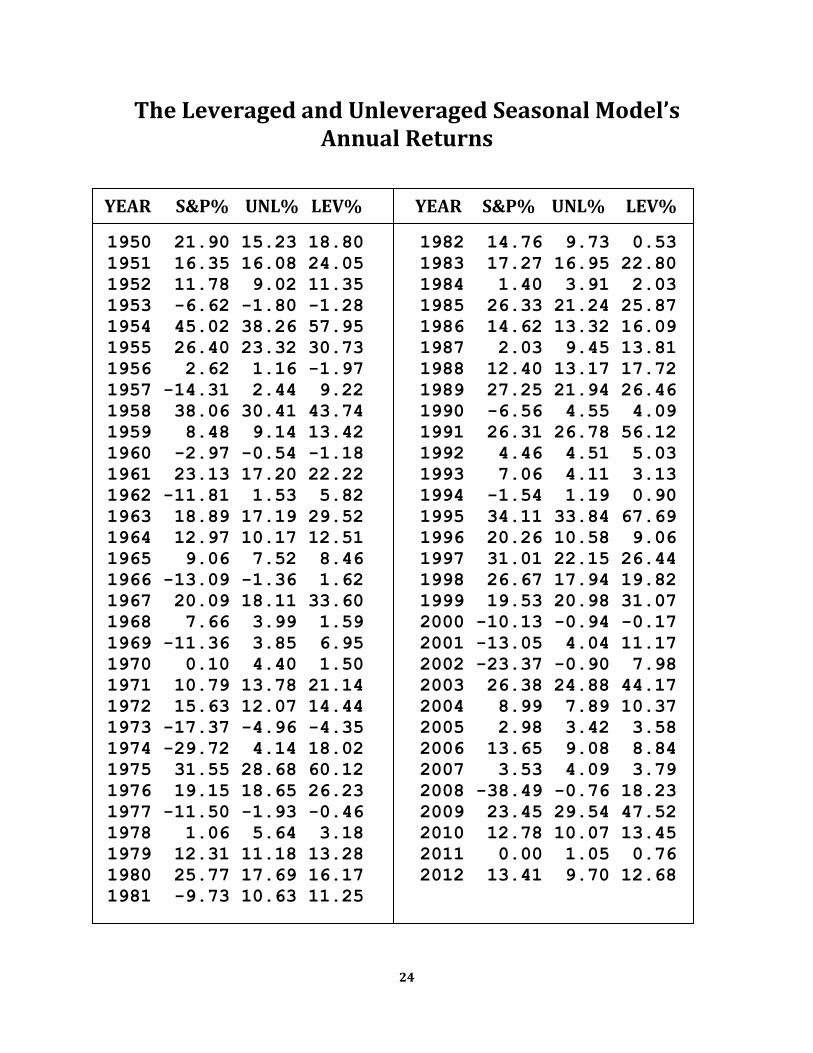
The Leveraged and Unleveraged Seasonal Model’s Annual Returns
YEAR S&P% UNL% LEV% YEAR S&P% UNL% LEV%
1950 21.90 15.23 18.80 1982 14.76 9.73 0.53
1951 16.35 16.08 24.05 1983 17.27 16.95 22.80
1952 11.78 9.02 11.35 1984 1.40 3.91 2.03
1953 -6.62 -1.80 -1.28 1985 26.33 21.24 25.87
1954 45.02 38.26 57.95 1986 14.62 13.32 16.09
1955 26.40 23.32 30.73 1987 2.03 9.45 13.81
1956 2.62 1.16 -1.97 1988 12.40 13.17 17.72
1957 -14.31 2.44 9.22 1989 27.25 21.94 26.46
1958 38.06 30.41 43.74 1990 -6.56 4.55 4.09
1959 8.48 9.14 13.42 1991 26.31 26.78 56.12
1960 -2.97 -0.54 -1.18 1992 4.46 4.51 5.03
1961 23.13 17.20 22.22 1993 7.06 4.11 3.13
1962 -11.81 1.53 5.82 1994 -1.54 1.19 0.90
1963 18.89 17.19 29.52 1995 34.11 33.84 67.69
1964 12.97 10.17 12.51 1996 20.26 10.58 9.06
1965 9.06 7.52 8.46 1997 31.01 22.15 26.44
1966 -13.09 -1.36 1.62 1998 26.67 17.94 19.82
1967 20.09 18.11 33.60 1999 19.53 20.98 31.07
1968 7.66 3.99 1.59 2000 -10.13 -0.94 -0.17
1969 -11.36 3.85 6.95 2001 -13.05 4.04 11.17
1970 0.10 4.40 1.50 2002 -23.37 -0.90 7.98
1971 10.79 13.78 21.14 2003 26.38 24.88 44.17
1972 15.63 12.07 14.44 2004 8.99 7.89 10.37
1973 -17.37 -4.96 -4.35 2005 2.98 3.42 3.58
1974 -29.72 4.14 18.02 2006 13.65 9.08 8.84
1975 31.55 28.68 60.12 2007 3.53 4.09 3.79
1976 19.15 18.65 26.23 2008 -38.49 -0.76 18.23
1977 -11.50 -1.93 -0.46 2009 23.45 29.54 47.52
1978 1.06 5.64 3.18 2010 12.78 10.07 13.45
1979 12.31 11.18 13.28 2011 0.00 1.05 0.76
1980 25.77 17.69 16.17 2012 13.41 9.70 12.68
1981 -9.73 10.63 11.25
24
Summary
1. Based on three different statistical measures examined, January is
the most reliable of the twelve calendar months in forecasting the
direction of the subsequent twelve months, but its ability to
provide guidance in sidestepping negative years is negligible.
2. If one does not constrain one’s seasonal barometer selection solely
to the twelve calendar months, or for that matter, monthly time
periods at all, the time period from November 19 through January
19 has a superior record to the traditional January Barometer in
forecasting the prospects for the S&P’s next twelve months. This
time period, which I have labeled the TOY (Turn of Year) period,
yields measurably better results predicting negative years, than
does the January Barometer with the 13 observed negative TOY
periods being followed by negative years in nine of those 13 cases.
Eleven of those 13 negative TOYs experienced a 12.5% drawdown
from the signal date at some point during the following year.
25
3. In a special Red Ryder TOY setup case, if a negative TOY Year
(January 19 – January 19), concludes with a positive TOY period
(November 19 – January 19), the following TOY year has been up at
least 10% in all ten occasions this setup has developed since 1950
and has caught five of the six +30% years, with an impressive ten
signal average/median annual return of 27.25/28.71.
4. Although not mentioned in this paper, the top dozen time frames
identified in the scan for the top seasonal barometer period of the
year all came from the mid November through mid February time
frame. For example, November 19 – February 5, was a close second
place. I did not find any other time periods outside of this three
month turn of year period which produced similar results.
5. The seasonal model, which I have introduced, has a very appealing
track record, but there are time frames, such as the fall of 87,
where one would also be well served to draw from other market
influences such as tape, interest rate influences, sentiment,
economic and valuation systems. A subject we will address in
more detail, tomorrow.
26
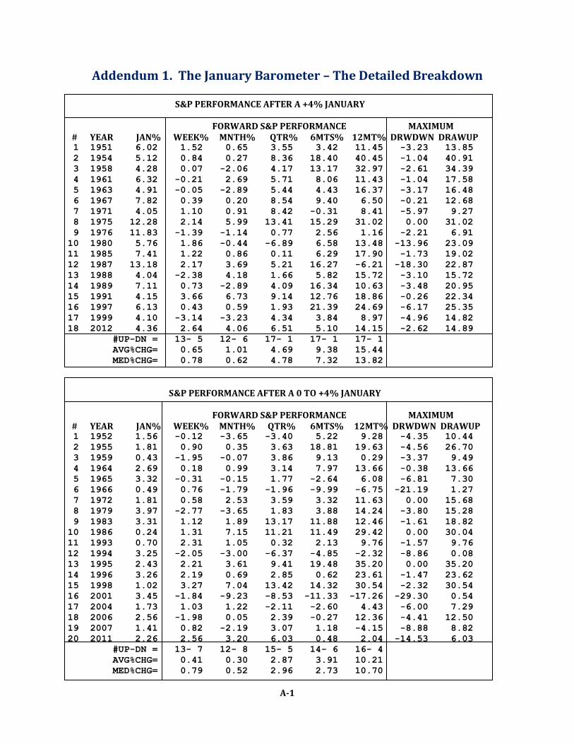
Addendum 1. The January Barometer – The Detailed Breakdown
S&P PERFORMANCE AFTER A +4% JANUARY FORWARD S&P PERFORMANCE MAXIMUM # YEAR JAN% WEEK% MNTH% QTR% 6MTS% 12MT% DRWDWN DRAWUP 1 1951 6.02 1.52 0.65 3.55 3.42 11.45 -3.23 13.85
2 1954 5.12 0.84 0.27 8.36 18.40 40.45 -1.04 40.91
3 1958 4.28 0.07 -2.06 4.17 13.17 32.97 -2.61 34.39
4 1961 6.32 -0.21 2.69 5.71 8.06 11.43 -1.04 17.58
5 1963 4.91 -0.05 -2.89 5.44 4.43 16.37 -3.17 16.48
6 1967 7.82 0.39 0.20 8.54 9.40 6.50 -0.21 12.68
7 1971 4.05 1.10 0.91 8.42 -0.31 8.41 -5.97 9.27
8 1975 12.28 2.14 5.99 13.41 15.29 31.02 0.00 31.02
9 1976 11.83 -1.39 -1.14 0.77 2.56 1.16 -2.21 6.91
10 1980 5.76 1.86 -0.44 -6.89 6.58 13.48 -13.96 23.09
11 1985 7.41 1.22 0.86 0.11 6.29 17.90 -1.73 19.02
12 1987 13.18 2.17 3.69 5.21 16.27 -6.21 -18.30 22.87
13 1988 4.04 -2.38 4.18 1.66 5.82 15.72 -3.10 15.72
14 1989 7.11 0.73 -2.89 4.09 16.34 10.63 -3.48 20.95
15 1991 4.15 3.66 6.73 9.14 12.76 18.86 -0.26 22.34
16 1997 6.13 0.43 0.59 1.93 21.39 24.69 -6.17 25.35
17 1999 4.10 -3.14 -3.23 4.34 3.84 8.97 -4.96 14.82
18 2012 4.36 2.64 4.06 6.51 5.10 14.15 -2.62 14.89
#UP-DN = 13- 5 12- 6 17- 1 17- 1 17- 1
AVG%CHG= 0.65 1.01 4.69 9.38 15.44
MED%CHG= 0.78 0.62 4.78 7.32 13.82
S&P PERFORMANCE AFTER A 0 TO +4% JANUARY FORWARD S&P PERFORMANCE MAXIMUM # YEAR JAN% WEEK% MNTH% QTR% 6MTS% 12MT% DRWDWN DRAWUP 1 1952 1.56 -0.12 -3.65 -3.40 5.22 9.28 -4.35 10.44
2 1955 1.81 0.90 0.35 3.63 18.81 19.63 -4.56 26.70
3 1959 0.43 -1.95 -0.07 3.86 9.13 0.29 -3.37 9.49
4 1964 2.69 0.18 0.99 3.14 7.97 13.66 -0.38 13.66
5 1965 3.32 -0.31 -0.15 1.77 -2.64 6.08 -6.81 7.30
6 1966 0.49 0.76 -1.79 -1.96 -9.99 -6.75 -21.19 1.27
7 1972 1.81 0.58 2.53 3.59 3.32 11.63 0.00 15.68
8 1979 3.97 -2.77 -3.65 1.83 3.88 14.24 -3.80 15.28
9 1983 3.31 1.12 1.89 13.17 11.88 12.46 -1.61 18.82
10 1986 0.24 1.31 7.15 11.21 11.49 29.42 0.00 30.04
11 1993 0.70 2.31 1.05 0.32 2.13 9.76 -1.57 9.76
12 1994 3.25 -2.05 -3.00 -6.37 -4.85 -2.32 -8.86 0.08
13 1995 2.43 2.21 3.61 9.41 19.48 35.20 0.00 35.20
14 1996 3.26 2.19 0.69 2.85 0.62 23.61 -1.47 23.62
15 1998 1.02 3.27 7.04 13.42 14.32 30.54 -2.32 30.54
16 2001 3.45 -1.84 -9.23 -8.53 -11.33 -17.26 -29.30 0.54
17 2004 1.73 1.03 1.22 -2.11 -2.60 4.43 -6.00 7.29
18 2006 2.56 -1.98 0.05 2.39 -0.27 12.36 -4.41 12.50
19 2007 1.41 0.82 -2.19 3.07 1.18 -4.15 -8.88 8.82
20 2011 2.26 2.56 3.20 6.03 0.48 2.04 -14.53 6.03
#UP-DN = 13- 7 12- 8 15- 5 14- 6 16- 4
AVG%CHG= 0.41 0.30 2.87 3.91 10.21
MED%CHG= 0.79 0.52 2.96 2.73 10.70
A-1
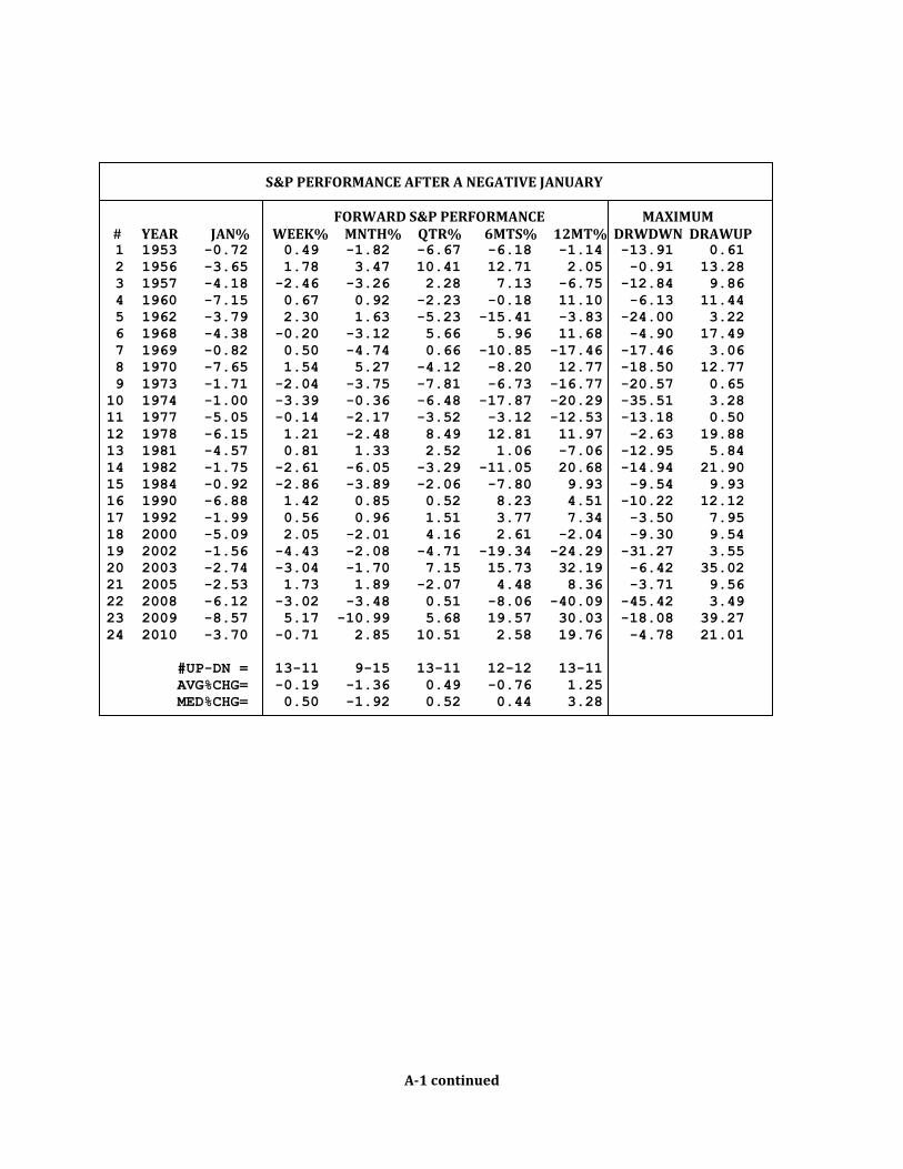
S&P PERFORMANCE AFTER A NEGATIVE JANUARY FORWARD S&P PERFORMANCE MAXIMUM # YEAR JAN% WEEK% MNTH% QTR% 6MTS% 12MT% DRWDWN DRAWUP 1 1953 -0.72 0.49 -1.82 -6.67 -6.18 -1.14 -13.91 0.61
2 1956 -3.65 1.78 3.47 10.41 12.71 2.05 -0.91 13.28
3 1957 -4.18 -2.46 -3.26 2.28 7.13 -6.75 -12.84 9.86
4 1960 -7.15 0.67 0.92 -2.23 -0.18 11.10 -6.13 11.44
5 1962 -3.79 2.30 1.63 -5.23 -15.41 -3.83 -24.00 3.22
6 1968 -4.38 -0.20 -3.12 5.66 5.96 11.68 -4.90 17.49
7 1969 -0.82 0.50 -4.74 0.66 -10.85 -17.46 -17.46 3.06
8 1970 -7.65 1.54 5.27 -4.12 -8.20 12.77 -18.50 12.77
9 1973 -1.71 -2.04 -3.75 -7.81 -6.73 -16.77 -20.57 0.65
10 1974 -1.00 -3.39 -0.36 -6.48 -17.87 -20.29 -35.51 3.28
11 1977 -5.05 -0.14 -2.17 -3.52 -3.12 -12.53 -13.18 0.50
12 1978 -6.15 1.21 -2.48 8.49 12.81 11.97 -2.63 19.88
13 1981 -4.57 0.81 1.33 2.52 1.06 -7.06 -12.95 5.84
14 1982 -1.75 -2.61 -6.05 -3.29 -11.05 20.68 -14.94 21.90
15 1984 -0.92 -2.86 -3.89 -2.06 -7.80 9.93 -9.54 9.93
16 1990 -6.88 1.42 0.85 0.52 8.23 4.51 -10.22 12.12
17 1992 -1.99 0.56 0.96 1.51 3.77 7.34 -3.50 7.95
18 2000 -5.09 2.05 -2.01 4.16 2.61 -2.04 -9.30 9.54
19 2002 -1.56 -4.43 -2.08 -4.71 -19.34 -24.29 -31.27 3.55
20 2003 -2.74 -3.04 -1.70 7.15 15.73 32.19 -6.42 35.02
21 2005 -2.53 1.73 1.89 -2.07 4.48 8.36 -3.71 9.56
22 2008 -6.12 -3.02 -3.48 0.51 -8.06 -40.09 -45.42 3.49
23 2009 -8.57 5.17 -10.99 5.68 19.57 30.03 -18.08 39.27
24 2010 -3.70 -0.71 2.85 10.51 2.58 19.76 -4.78 21.01
#UP-DN = 13-11 9-15 13-11 12-12 13-11
AVG%CHG= -0.19 -1.36 0.49 -0.76 1.25
MED%CHG= 0.50 -1.92 0.52 0.44 3.28
A-1 continued
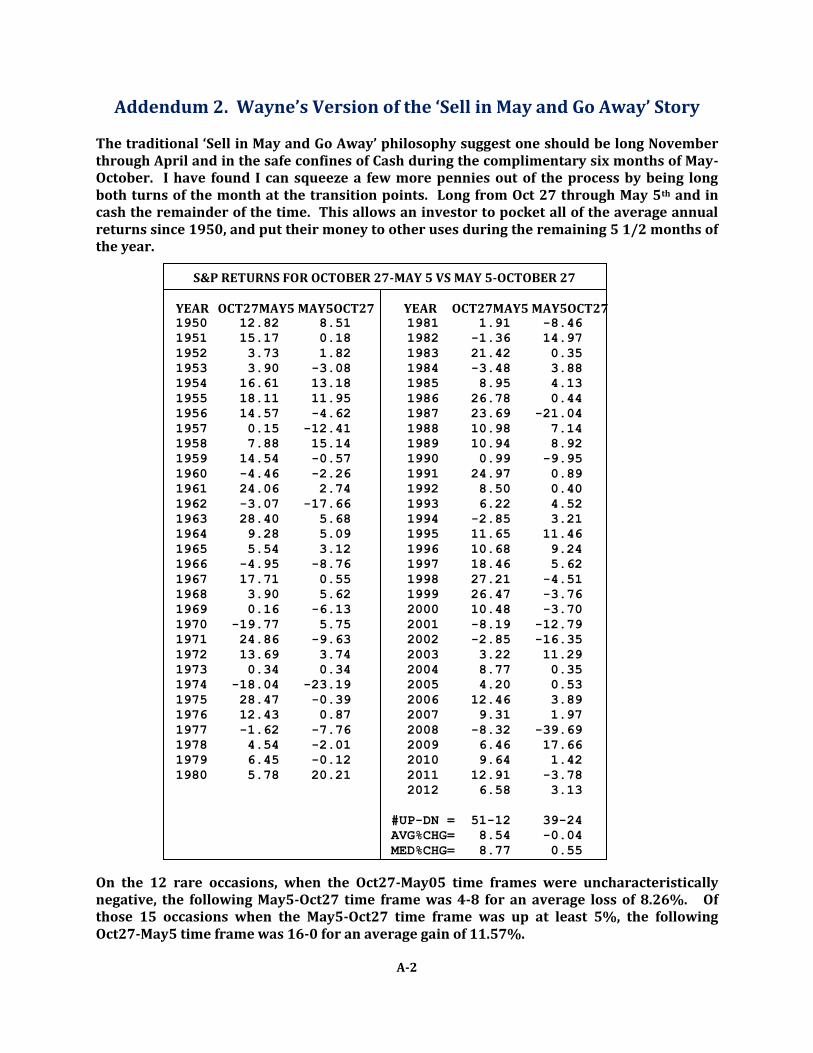
Addendum 2. Wayne’s Version of the ‘Sell in May and Go Away’ Story The traditional ‘Sell in May and Go Away’ philosophy suggest one should be long November through April and in the safe confines of Cash during the complimentary six months of May- October. I have found I can squeeze a few more pennies out of the process by being long both turns of the month at the transition points. Long from Oct 27 through May 5th and in cash the remainder of the time. This allows an investor to pocket all of the average annual returns since 1950, and put their money to other uses during the remaining 5 1/2 months of the year.
S&P RETURNS FOR OCTOBER 27-MAY 5 VS MAY 5-OCTOBER 27
YEAR OCT27MAY5 MAY5OCT27 YEAR OCT27MAY5 MAY5OCT27 1950 12.82 8.51 1981 1.91 -8.46
1951 15.17 0.18 1982 -1.36 14.97
1952 3.73 1.82 1983 21.42 0.35
1953 3.90 -3.08 1984 -3.48 3.88
1954 16.61 13.18 1985 8.95 4.13
1955 18.11 11.95 1986 26.78 0.44
1956 14.57 -4.62 1987 23.69 -21.04
1957 0.15 -12.41 1988 10.98 7.14
1958 7.88 15.14 1989 10.94 8.92
1959 14.54 -0.57 1990 0.99 -9.95
1960 -4.46 -2.26 1991 24.97 0.89
1961 24.06 2.74 1992 8.50 0.40
1962 -3.07 -17.66 1993 6.22 4.52
1963 28.40 5.68 1994 -2.85 3.21
1964 9.28 5.09 1995 11.65 11.46
1965 5.54 3.12 1996 10.68 9.24
1966 -4.95 -8.76 1997 18.46 5.62
1967 17.71 0.55 1998 27.21 -4.51
1968 3.90 5.62 1999 26.47 -3.76
1969 0.16 -6.13 2000 10.48 -3.70
1970 -19.77 5.75 2001 -8.19 -12.79
1971 24.86 -9.63 2002 -2.85 -16.35
1972 13.69 3.74 2003 3.22 11.29
1973 0.34 0.34 2004 8.77 0.35
1974 -18.04 -23.19 2005 4.20 0.53
1975 28.47 -0.39 2006 12.46 3.89
1976 12.43 0.87 2007 9.31 1.97
1977 -1.62 -7.76 2008 -8.32 -39.69
1978 4.54 -2.01 2009 6.46 17.66
1979 6.45 -0.12 2010 9.64 1.42
1980 5.78 20.21 2011 12.91 -3.78
2012 6.58 3.13
#UP-DN = 51-12 39-24
AVG%CHG= 8.54 -0.04
MED%CHG= 8.77 0.55
On the 12 rare occasions, when the Oct27-May05 time frames were uncharacteristically negative, the following May5-Oct27 time frame was 4-8 for an average loss of 8.26%. Of those 15 occasions when the May5-Oct27 time frame was up at least 5%, the following Oct27-May5 time frame was 16-0 for an average gain of 11.57%.
A-2

Addendum 3. 2013 Election Cycle Analysis
It is a well documented phenomenon that equities tend to perform better in the second half of the four year election cycle than in the first two years, particularly the PreElection Year, which has shown a profit in 18 of those 21 years since 1930, for an average/median gain of 13.44/17.27%. Some have been brave enough to venture that there are political shenanigans contributing to such peculiarities. Since we only get one data point each four years, I extended this study back to the extent of my S&P database (1930). ELECTION CYCLE RESULTS 1930-2012 POST ELECTION MID ELECTION PRE ELECTION ELECTION YEAR YEAR PCTCH YEAR PCTCH YEAR PCTCH YEAR PCTCH 1930 -27.57 1931 -47.07 1932 -15.15
1933 46.59 1934 -5.94 1935 41.37 1936 27.92
1937 -38.59 1938 25.21 1939 -5.45 1940 -15.29
1941 -17.86 1942 12.43 1943 19.45 1944 13.80
1945 30.72 1946 -11.87 1947 0.00 1948 -0.65
1949 10.26 1950 21.90 1951 16.35 1952 11.78
1953 -6.62 1954 45.02 1955 26.40 1956 2.62
1957 -14.31 1958 38.06 1959 8.48 1960 -2.97
1961 23.13 1962 -11.81 1963 18.89 1964 12.97
1965 9.06 1966 -13.09 1967 20.09 1968 7.66
1969 -11.36 1970 0.10 1971 10.79 1972 15.63
1973 -17.37 1974 -29.72 1975 31.55 1976 19.15
1977 -11.50 1978 1.06 1979 12.31 1980 25.77
1981 -9.73 1982 14.76 1983 17.27 1984 1.40
1985 26.33 1986 14.62 1987 2.03 1988 12.40
1989 27.25 1990 -6.56 1991 26.31 1992 4.46
1993 7.06 1994 -1.54 1995 34.11 1996 20.26
1997 31.01 1998 26.67 1999 19.53 2000 -10.13
2001 -13.05 2002 -23.37 2003 26.38 2004 8.99
2005 2.98 2006 13.64 2007 3.53 2008 -38.49
2009 23.45 2010 12.78 2011 0.00 2012 13.41
#UP-DN = 11- 9 #UP-DN = 12- 9 #UP-DN =18- 3 #UP-DN = 15- 6
AVG%CHG= 4.87 AVG%CHG= 4.51 AVG%CHG=13.44 AVG%CHG= 5.50
AVG%CHG= 5.02 MED%CHG= 1.06 MED%CHG=17.27 MED%CHG= 8.99
And although, it is the general perception that Republican administrations are more business friendly than Democratic, for whatever reasons you care to postulate, post 1929 equity prices have prospered better under Democratic Administrations. S&P ANNUAL PEFORMANCE VS PRESEDENTIAL PARTY
PARTY #UP-DN %UP AVG% MED% DEMOCRATIC 31-13 70.5 10.30 12.61
REPUBLICAN 25-14 64.1 3.51 3.53
A-3

Addendum 4. The Wayne Whaley Story
Wayne Whaley, CTA, received a Masters Degree in Operations
Research in 1981 from the Georgia Institute of Technology,
where he received his first exposure to the mathematical
modeling of probabilistic models. His education also focused
on Optimization Theory, Time Series Analysis, Simulation
Techniques and Game Theory. Wayne had little idea at the time
where his applied mathematics background would lead him,
but even as a student, he had a special fondness for his Engineering Economics classes.
After college, Wayne migrated to Huntsville, AL, where he was employed from 1981-1993 as
a system analyst for Teledyne Brown Engineering and Sparta Inc. Wayne honed his
programming and analytical skills during the 80’s ‘Strategic Defense Initiative ’ exercise by
leading efforts to develop software that simulated the outcome of two sided nuclear force
exchanges between the Soviet Union and the United States. Wayne’s hobby during this time
was the mathematical modeling of the stock market and he eventually joined Witter &
Lester, a Huntsville, Alabama, based Commodity Trading Advisor (CTA), in 1993 as a
research analyst with the intention of turning his hobby into a career.
Wayne became a partner at Witter & Lester in 1999. Although, he now trades the company’s
assets, he still considers himself to be the research department, with trading merely serving
as the eventual report card for his research efforts. Mr. Whaley’s forte is the
implementation of his engineering background in the development of pattern recognition
techniques, along with the ability to backtest multitudes of combinations of candidate
market strategies. He currently utilizes a 20,000 line computer code that he has been
developing over the last 15 years to aid him in his market decisions. The model relies
predominantly on its ability to take an electronic snapshot each day of an indicator’s
characteristics, identifying all similar instances in the past, and summarizing the statistical
results for the user.
Wayne has a fondness for spinning a tale and was the recipient of the 2010 Charles Dow
Award from the Market Technicians Association for his research paper, ‘Planes, Trains, &
Automobiles, a Survey or Momentum Thrust Signals’, which is posted online. Wayne writes
weekly market commentary and has been published in ‘Technical Analysis of Stocks and
Commodities’, ‘Futures Magazine’, and referenced in Barron’s. A Google of his name will
produce many of his daily studies which have found their way into circulation on
cyberspace.
Wayne Whaley, Witter& Lester Inc., 3330E L&N Dr., Huntsville, AL. 35801,
A-4