Embed Size (px)
Citation preview
A RE-EXAMINATION OF THE DEMAND FOR
MONEY IN FIJI
Resina Katafono
Working Paper2001/03
May 2001
Economics Department
Reserve Bank of Fiji
Suva
Fiji
The views expressed herein are those of the author and do not necessarilyreflect those of the Reserve Bank of Fiji. The author expresses her thanksto Steven Morling, Caroline Waqabaca, Sylvia Sivo and Barry Whiteside ofthe Reserve Bank for their valuable comments.

Abstract
The failure of conventional money demand functions in a number
of countries has resulted in the downgrading of monetary aggregates in the
conduct of monetary policy. Although prior studies have been conducted
on the demand for money in Fiji, the results have been mixed. This paper
seeks to use contemporary empirical methods to model the demand for
money based on sound theoretical principles. The paper reviews some
basic concepts of money demand theory, reviews model specification
issues, and summarises the results of developed and developing countries’
studies that have used cointegration and/or error correction techniques. In
addition, the study tests for the existence of cointegration between a
number of monetary aggregates, economic activity and interest rates. The
error correction method is also used to support the cointegration findings.
The empirical findings conclude that the demand for money in Fiji is
unstable.

2
1.0 Introduction
The demand for money is at the heart of how policy should be
conducted effectively. Money demand serves as a conduit in the
transmission mechanism for monetary policy so the stability of the money
demand function is critical if monetary policy is to have predictable effects
on inflation and real output. In most developed and developing countries,
policymakers have frequently questioned whether the demand for money is
stable. Generally, the majority of studies find that the demand for money is
unstable and monetary aggregates have lost their influence in the conduct
of monetary policy.
In Fiji, for sometime, the role of monetary aggregates as
intermediate targets has been downplayed. However, there has been
renewed interest in the stability of the demand for money in Fiji and so this
paper's objective is to re-examine this topical issue. Because of ongoing
financial sector reforms1, the determinants of money demand in Fiji will be
difficult to establish. Nevertheless, this paper aims to provide a sound
theoretical and empirical basis for modelling the demand for money. This
paper employs cointegration analysis to examine the stability of the
demand for money. Additionally, the error correction technique is also
used to confirm the findings of the cointegration analysis.
The paper is divided into three parts. In the first part of the paper,
the empirical survey covers the theories of money demand, selection of
variables and model specifications. In addition, this part also outlines
recent findings from both developed and developing countries as well as
1 See Waqabaca (2000) for a detailed account of the financial sector reforms implemented so far.

3
studies done on the demand for money in Fiji. The second part of the paper
outlines the model used in the study and discusses the results obtained from
this model. The third part concludes the study.
2.0 Empirical Survey
The theory of money demand is one of the most enduring issues in
economics and as such, the empirical literature and research available is
very large. It is beyond the scope of this paper to address all the issues
related to the demand for money. However, this section will briefly cover
four areas – (1) theories of money demand, (2) selection of variables, (3)
specification issues and lastly, (4) the latest empirical findings2.
2.1 Theories of Money Demand
2.1.1 Classical Theories
According to classical economists, money acts as a numéraire. In
other words, it is a commodity whose unit is used in order to express prices
and values, but whose own value remains unaffected by this role (Sriram,
1999). However, money is deemed neutral with no real economic
consequences since its role as a store of value, is limited under the classical
assumption of perfect information and negligible transaction costs (Sriram,
1999).
The roots of modern theory of money demand began from the early
contributions of Mill (1848), Walras (1900) and Wicksell (1906). The
2 Majority of the works quoted in these sections was cited in Sriram (1999).

4
concept of money demand took formal shape through the quantity theory
developed in the classical equilibrium framework by two different but
equivalent expressions.
Fisher (1911) provided the famous equation of exchange (MsVt =
PtT, where Ms is quantity of money, Vt is the transactions velocity of
circulation, Pt is prices and T the volume of transactions) where money is
held simply to facilitate transactions and has no intrinsic value. The
alternative paradigm, the so-called Cambridge approach, was primarily
associated with the neo-classical economists Pigou (1917) and Marshall
(1923). This approach stressed the demand for money as public demand
for money holdings, especially the demand for real balances, which was an
important factor in determining the equilibrium price level consistent with a
given quantity of money (Sriram, 1999).
2.1.2 Keynesian Theory
Keynes (1930, 1936) built upon the Cambridge approach to provide
a more rigorous analysis of money demand, focussing on the motives of
holding money. Keynes postulated three motives for holding money:
transactions, precautionary and speculative purposes. He also formally
introduced the interest rate as another explanatory variable in influencing
the demand for real balances.
The money demand function was then represented as ),( iyfmd =
where the demand for real balances (md) is a function of real income (y)
and nominal interest rates (i). The main proposition of the Keynesian
analysis is that when interest rates are low, economic agents will expect a
future increase in interest rates; thus, preferring to hold whatever amount of

5
money is supplied. Therefore, the aggregate demand for money becomes
perfectly elastic with respect to the interest rate (liquidity trap).
2.1.3 Post-Keynes
Following Keynes, a number of models were developed to confirm
the relationship between the demand for real money and, income and
interest rates. These models can be classified into three separate
frameworks, namely transactions, asset and consumer demand theories of
money.
Under the transactions theory of money demand framework, the
inventory-theoretic approach (see Baumol, 1952 and Tobin, 1956) and the
precautionary demand for money (see inter alia Cuthbertson and Barlow,
1991) models were introduced. These models were derived from the
medium-of-exchange function of money.
The asset function of money led to the asset or portfolio approach
where major emphasis is placed on risk and expected returns of assets (see
Tobin, 1958). Alternatively, the consumer demand theory approach (see
Friedman, 1956 and Barnett, 1980) considers the demand for money as a
direct extension of the traditional theory of demand for any durable good
(see Feige and Pearce, 1977).
The resulting implication of all the models discussed in the
previous sections is that the optimal stock of real money balances is
positively related to real income and inversely related to the nominal rate of
return. Ultimately, the difference lies in the selection of variables that will
enter the model.

6
2.2 Selection of Variables
2.2.1 Money Stock
Money stocks are mainly classified into two groups – narrow and
broad money. As the name suggests, narrow money consists of those assets
readily available for transactions while broad money encompasses a wider
range of assets. Laidler (1993) states that the correct definition of money is
an empirical matter. As such, several definitions of money have been used
in various studies. The measures of money have been selected based on the
objectives of the researchers (Sriram, 1999). For the purposes of this paper,
the three widely used measures of money in Fiji (namely, narrow money,
quasi money and broad money) are used to discover if there is a stable
demand function for either of the measures.
2.2.2 Scale Variable
The scale variable is used as a gauge of transactions relating to
economic activity. The most commonly used variables are gross national
product (GNP) and other related variables such as gross domestic product
(GDP) and net national product (NNP). Recent research have focussed on
other scale variables involving more comprehensive measures of
transactions and the segregation of transactions into various components
under the idea that all transactions are not equally ‘money intensive’ (see
Goldfeld and Sichel, 1990). However, Goldfeld and Sichel (1990)
concluded that there is no firm evidence that the categorisation of GNP into
components yields an improvement in the behaviour of money demand.
Wealth has also been used as a scale variable but usage has been

7
constrained to only a few countries such as the United Kingdom and the
United States where data is available. This paper uses real GDP as a proxy
for the scale variable as the data is readily available and it satisfies both the
income and wealth criteria that the scale variable should represent.
2.2.3 Opportunity Cost Variables
Typically, the opportunity cost of holding money involves two
components, the own rate of return of money and the rate of return on
alternative assets. Ericsson (1998) states that it is important to include both
interest rates to avoid the collapse of the estimated money demand
function. Considering portfolio choices, agents also consider money as part
of real and foreign assets (Sriram, 1999).
The return on real assets is usually represented by the expected rate
of inflation (Sriram, 1999). Theoretically, Friedman (1956, 1969)
pioneered the inclusion of the expected rate of inflation, and the
relationship between demand for money and expected inflation is well
documented by Arestis (1988). Arestis postulated that the real value of
money falls with inflation whilst the value of real assets is maintained.
Therefore, there is a strong incentive for persons to switch out of money
and into real assets when there are strong inflationary expectations. In
developing countries where the financial sector is not well developed, the
expected rate of inflation is usually the only variable used as the
opportunity cost of holding money3.
3 There are two major reasons (relevant in Fiji’s case) for including expected inflation. (1) There isnarrow substitution between money and other financial assets as the financial sector is under-developedand (2) interest rates may show insufficient variation due to regulation (see inter alia Wong, 1977).

8
Foreign interest rates and the expected rate of depreciation usually
represent the returns on foreign assets (Sriram, 1999). The currency
substitution literature provides the necessary support in choosing the
appropriate variables that account for foreign influence. Direct currency
substitution concentrates on the exchange rate variable while the capital
mobility or indirect currency substitution literature focuses on foreign
interest rates (see inter alia Giovannini and Turtelboom, 1993 and
Leventakis, 1993).
For the purposes of this paper, both the own rate of return of money
and the rate of return of the alternative asset is included. The nominal rate
is used since there are two costs associated with holding money balances –
the real interest rate reflects the opportunity cost of holding deposits, while
the expected rate of inflation is to compensate depositors for the expected
depreciation in the real value of money because of inflation. Following
Bahmani-Oskooee (1991), the real effective exchange rate is used as a
proxy for expected depreciation. The foreign interest rate was disregarded
as it is assumed that most economic agents in Fiji do not consider foreign
securities as a relevant investment alternative, mainly due to the existence
of exchange controls.
2.3 Specifications
2.3.1 Partial Adjustment Models (PAM)
The PAM, a log-linear specification extensively used for estimating
money demand, was originally introduced by Chow (1966) and later
popularised by Goldfeld (1973). This model augments the traditional
formulation of money demand by introducing the following two concepts:

9
(i) distinction between desired and actual money holdings and (ii) the
system by which the actual money holdings adjust to the desired levels
(Sriram, 1999).
This model faired well when the post-war to 1973 data was used
but it was unable to explain the instability in the demand for money
experienced since the early 1970s (Sriram, 1999). The problems associated
with this model were both theoretical4 and empirical 5 in nature. The PAM
soon lost favour to the buffer stock models (BSM) and error correction
models (ECM). Boughton and Tavlas (1991) found that estimates obtained
by the BSM and ECM for money demand significantly outperformed those
of the PAM.
2.3.2 Buffer Stock Models
The BSM were predominant in the 1980s as an alternative
paradigm for money demand estimation to overcome the two common
problems with the PAM, namely the short-run interest overshooting and
long implausible lags of adjustment (Sriram, 1999). Proponents of BSM
postulated that the reason the PAM did poorly was that they failed to
consider the short-run impact of monetary shocks (Sriram, 1999). The two
main changes in the BSM over the PAM were that money shocks are
explicitly modelled as part of the determination of money demand and the
lag structure is much more complex (Sriram, 1999).
Despite the improvement made over the PAM, there have been
4 See Goodfriend (1985).
5 See inter alia Yoshida (1990) and Hendry and Doornik (1996).

10
mixed results in the empirical application of this approach (see Boughton
and Tavlas, 1991 and Cuthbertson and Taylor, 1987). Milbourne (1988)
concluded from his extensive survey that BSM had theoretical and
empirical shortcomings. Consequently, as criticisms grew, the BSM lost
their appeal while ECM moved to the forefront in estimating the demand
for money.
2.3.3 Error Correction Models
The ECM has proved to be a successful tool in applied money
demand research (Sriram, 1999). It is a dynamic error-correction
representation where the long-run equilibrium is embedded in an equation
that captures short-run variation and dynamics (see Kole and Meade, 1995).
Granger (1983, 1986) showed that the concept of stable long-term
equilibrium is the statistical equivalence of cointegration. Engle and
Granger (1987) state that cointegration implies the existence of a dynamic
error-correction form.
In regards to the estimation techniques, the two widely used
approaches are Engle and Granger (1987); and Johansen (1988) and
Johansen and Juselius (1990). The latter approach is more prominent as it
provides an opportunity to evaluate the presence of multiple cointegrating
vectors and has shown that it is more efficient than the former (Sriram,
1999).
Since the necessary precondition for the existence of a long-run
relationship is the presence of a cointegrating vector, the empirical section
begins with the cointegration analysis. When the cointegration
relationships are found, weak exogeneity tests are done to explore whether
11
the models can be reduced from a system to a single equation to analyse the
short-run dynamics. However, before proceeding to the empirical section,
the next section briefly summarises recent research results. The next
section will also discuss the results of the studies done on the demand for
money in Fiji.
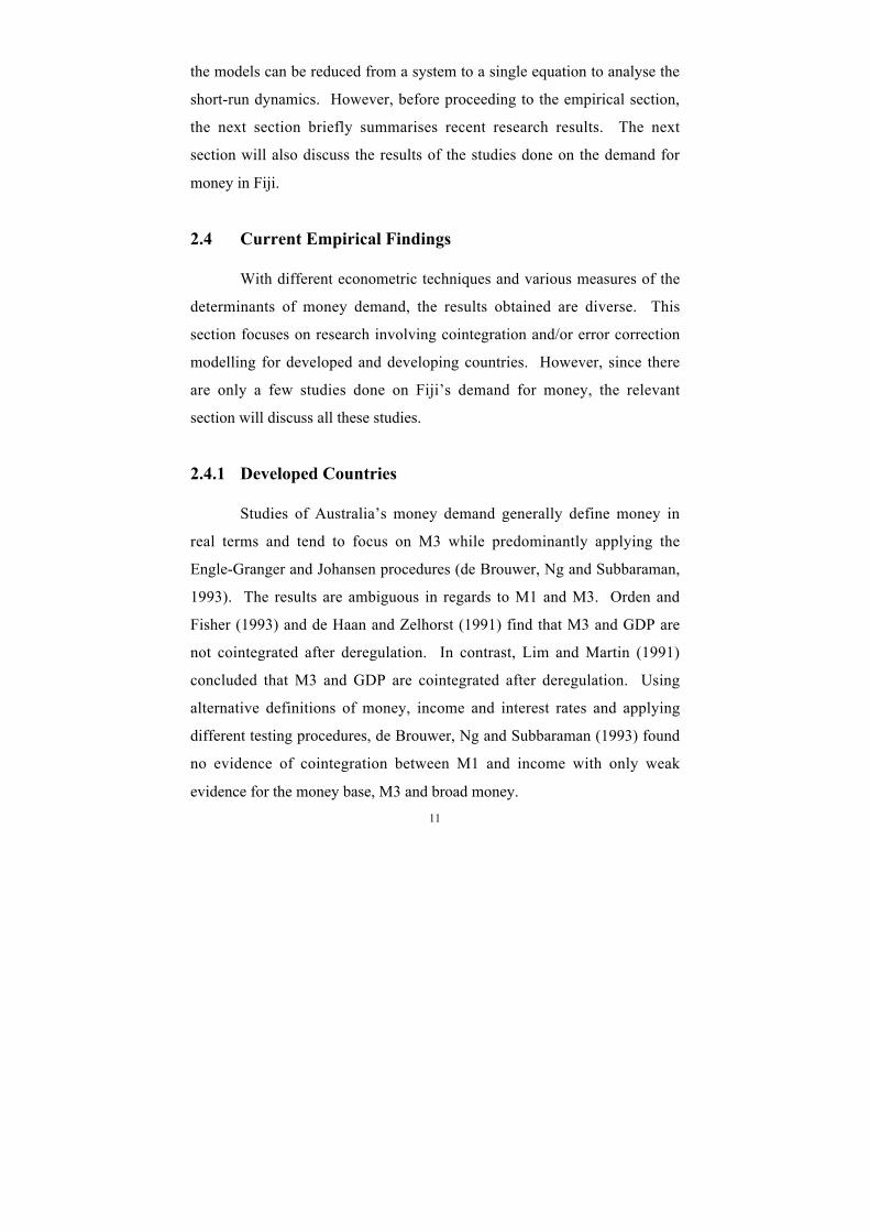
2.4 Current Empirical Findings
With different econometric techniques and various measures of the
determinants of money demand, the results obtained are diverse. This
section focuses on research involving cointegration and/or error correction
modelling for developed and developing countries. However, since there
are only a few studies done on Fiji’s demand for money, the relevant
section will discuss all these studies.
2.4.1 Developed Countries
Studies of Australia’s money demand generally define money in
real terms and tend to focus on M3 while predominantly applying the
Engle-Granger and Johansen procedures (de Brouwer, Ng and Subbaraman,
1993). The results are ambiguous in regards to M1 and M3. Orden and
Fisher (1993) and de Haan and Zelhorst (1991) find that M3 and GDP are
not cointegrated after deregulation. In contrast, Lim and Martin (1991)
concluded that M3 and GDP are cointegrated after deregulation. Using
alternative definitions of money, income and interest rates and applying
different testing procedures, de Brouwer, Ng and Subbaraman (1993) found
no evidence of cointegration between M1 and income with only weak
evidence for the money base, M3 and broad money.

12
For New Zealand, Orden and Fisher (1993) found no cointegrating
relationship for the full sample (quarterly data between 1965 and 1984).
Similarly, applying Canadian data from 1968 to 1999, Tkacz (2000) found
that money, output, prices and interest rates are only fractionally
cointegrated.
However, in the United Kingdom, Drake and Chrystal (1994) found
that a cointegrating relationship existed for all the monetary aggregates
examined and the ECM indicated a rapid speed of adjustment. The latter
results were mirrored in Miller’s (1991) study in the US where he found a
cointegration relationship for M2 and the ECM for M2 suggested a
significant error-correction term. Hayo (1998) found a stable money
demand for 11 European Monetary Union (EMU) countries. Factoring
financial innovation, Scharnagl (1998) still found a stable long-run money
demand relationship for Germany.
From these few studies, it is evident that the results vary. Much of
the variation is dependent on the cointegration tests selected and the
combination of money and interest rates (Haug and Lucas, 1996).
Nevertheless, existence of cointegration between money and income would
not, in itself, necessarily establish a paramount role for monetary
aggregates in policy making (de Brouwer, Ng and Subbaraman, 1993).
Presently, central banks generally agree that conventional monetary
aggregates are of little use as targets or indicators for monetary policy
(Woodford, 1997). Woodford (1997) also contends that it is possible to
analyse equilibrium inflation determination without reference to money
supply or demand, “as long as one specifies policy in terms of a
‘Wicksellian’ interest-rate feedback rule”.
The next section investigates the results for money demand in

13
developing countries. Since the financial markets are less developed and
prone to regulation, the findings could be different.
2.4.2 Developing Countries
A money demand function was estimated for ten developing
countries (including India, Mexico and Nigeria) and cointegration was only
established in a minority of cases (Arrau et al, 1991). The instability of the
money demand function in the latter study was probably a result of the
failure to account for financial innovation (Arrau et al, 1991). However,
including proxies for financial innovation in the study did not improve the
stability of the demand for money in those developing countries. The
findings in this study suggest that while it is difficult to forecast the path of
financial innovation, it would be beneficial to model the process in some
way so as to recover better estimates of the money demand function (Arrau
et al, 1991).
In contrast, a stable relationship for narrow money was found for
the West African Economic and Monetary Union (WAEMU6) even amidst
financial liberalisation (Rother, 1998). However, Rother (1998) contends
that the stability of the demand for money would only continue in
WAEMU as long as the economic agents have confidence in the stability of
the financial system.
On the other hand, for the Association of South East Asian Nations
(ASEAN) countries, Dekle and Pradhan (1997) found continuing instability
in the demand for money as financial liberalisation intensified. The results
6 Countries included: Bénin, Burkina Faso, Côte d’Ivoire, Mali, Niger, Senegal, and Togo.

14
indicated that money growth rates were poor predictors of future inflation
and output trends, so policy decisions needed to be based on a wider set of
monetary and real sector indicators of inflationary pressures (Dekle and
Pradhan, 1997).
These studies and many others not covered in this paper indicate
that financial liberalisation is an important determinant of the stability of
money demand. However, as to its effect on the demand for money, the
results differ across countries. In addition, financial innovation is difficult
to measure and a reliable proxy is quite difficult to find.
This paper does not examine the effects of financial innovation on
money demand in Fiji as the financial markets are still at an embryonic
stage. However, as Fiji’s financial market develops, financial innovation
will play an important role in the demand for money and will need to be
included in future studies of money demand. Previous studies on the
demand for money in Fiji are outlined in the next section.
2.4.3 Money Demand in Fiji
There have only been a few studies done on the demand for money
in Fiji. The International Monetary Fund (IMF) conducted a study on the
demand for money in Fiji in 1982. The IMF model of the demand for
money was as follows:
)](,,[ ed
rYcfP
MP-=
where c is the constant, Y is income and ( er P- ) is the expected real rate
of return on time deposits. The results signal unitary income elasticity for
income whereas the interest rate elasticity was not statistically significant.

15
However, the results from this study are dubious in that it suffers from a
serious theoretical shortcoming. This study uses the real interest rate as a
determinant of the demand for real money balances. However, it is widely
recognised that the nominal interest rate is the appropriate determinant of
the demand for real money balances (Sachs and Larrain, 1993).
In 1987, Luckett (1987) also modelled the demand for money. This
time, the interest rate and expected inflation was separated:
],,,[ ed
rYcfP
MP=
Due to unavailability of data, Luckett (1987) used proxies for the interest
rate, r, such as the interbank rate, adjusted liquid assets margin ratio and the
loans and advances ratio. However, this study also suffered from
theoretical as well as empirical difficulties. As r is the nominal rate, it
already has expected inflation in it, so the coefficient on the expected
inflation term ( eP ) is not expected to pick up anything meaningful. The
interest rate proxy was also constrained to only six years of unregulated
data.
In addition, although the use of the adjusted liquid assets margin
and the loans and advances ratio is representative of the interest rates of
money, these proxies are themselves dependent on money balances.
Therefore, the latter has the effect of possibly introducing endogeneity in
the model. These concerns cast doubt on the results of Luckett's (1987)
findings that no substantial conclusion could be made on the demand for
money in Fiji.
In contrast, a recent study by Joynson (1997), applying the error
correction technique and the Johansen methodology, found weak results for
the demand for money. Joynson (1997) modelled the demand for real

16
money balances as a function of income (real GDP) and the interest rate
(proxies used were the one year weighted average savings deposit rate, the
treasury bill rate and the lending rate).
However, the latest study on the demand for money by Jayaraman
and Ward (2000) point towards a stable money demand function. In
Jayaraman and Ward's (2000) study, the money demand function was
expressed as:
LRM2t=b1+b2LRGDPt+b3RRt+b4LREERt+b5INFt+et
where LRM2 is the logarithm of real broad money, LRGDP is the
logarithm of real GDP, RR is the real interest rate, INF is the rate of
inflation and LREER is the logarithm of the real effective exchange rate.
The authors applied a quarterly series to the model although GDP
data is only available annually. To combat this problem, Jayaraman and
Ward (2000) have interpolated the quarterly data from the annual series
using a cubic spline function. However, basing a stable money demand
function on a quarterly series, where the GDP data is statistically
manipulated, biases the findings and interpretations and it will also provide
problems when trying to forecast the monetary aggregates. For
policymakers, a stable money demand function is only useful when it is
used for forecasting purposes and this will be difficult as it will be hard to
forecast GDP on a quarterly basis.
Considering the shortcomings of some of the previous studies, this
paper will serve to provide a stronger theoretical basis on which a model
for money demand is based. In addition, all empirical considerations will
be addressed, to ensure the robustness of the results.

17
3.0 Model
The money demand function is estimated in log-linear form. All
the variables, except the savings and treasury bill rate, enter the model in
logarithms. The basic framework of the model is as follows:
LRM=a1+a2LRGDP+a3SVR+a4TBR+a5LREER+e
where LRM is the ln (measure of money/CPI)
LRGDP is the ln (real gross domestic product)
SVR is the savings deposit rate
TBR is the treasury bill rate
LREER is the ln (real effective exchange rate)
Real gross domestic product is used as a proxy for the scale
variable. It is expected to be positively related to the real demand for
money. An increase in economic or transactions activity would necessitate
a greater demand for money. The coefficient of the savings rate is also
expected to be positive since it represents the interest rate of money. With
higher savings rates, the incentive to hold alternative assets will be lower.
Consequently, higher rates on the alternative asset will lead to a
disincentive for holding money. Therefore, the coefficient of the treasury
bill rate is expected to be negative. The real effective exchange rate (proxy
for the expected rate of depreciation) will also have a negative relationship
with money. An increase in expected depreciation would lead individuals
to substitute domestic currency for foreign currency under the implication
that expected returns from holding foreign currency will increase.

18
3.1 Data
Most data series are available from 1966 except for the savings and
treasury bill rate, which are only available from 1975. Therefore, the paper
applies annual data from 1975 to 19997. Before proceeding to the
cointegration analysis, the unit root characteristics of the data are
examined.
Augmented Dickey-Fuller (ADF) and Phillips-Perron (PP)8 unit
root tests are carried out on the series. The results suggest that all
variables, except for prices, appear to be integrated of order one. The
estimated roots for DPrices is numerically much less than unity9 so all the
variables are treated as I(1).
Table 1: Unit Root Tests
Dickey-Fuller Test Phillips-Perron TestVariables
I (1) I (2) I (1) I (2)
Real Broad Money -1.075 -3.627** -1.084 -5.167**
Real M1 0.585 -4.102** 0.773 -5.892**
Real Quasi Money -1.751 -3.268** -1.905 -4.686**
Real GDP 0.313 -5.378** 0.448 -7.866**
Prices -2.364 -2.400 -4.041** -2.506
Savings Rate -0.087 -2.178 0.081 -2.981*
Treasury Bill Rate -1.595 -4.853** -2.445 -7.639**
REER -0.882 -2.960* -0.714 -3.791**
An **(*) indicates rejection of hypothesis of a unit root at the five (ten) percent level.
7 See Appendix A for a detailed description of the data.
8 See Dickey & Fuller (1979) and Phillips & Perron (1988).
9 Using ADF tests, the estimated coefficient on the lagged price variable pt-1 is –0.41. Therefore, theestimated root is 0.59 (1-0.41). The PP results similarly conclude that the estimated root is numericallyless than unity.

19
The time series for the variables were examined graphically10 in
order to observe any drifts or structural breaks that may bias the unit root
tests. It is evident from the graphs that there are no noticeable breaks,
which supports the unit root test results.
3.2 Cointegration Analysis
Since the variables are considered to be I(1), the cointegration method is
appropriate to estimate the long-run demand for money. The cointegration
technique helps to clarify the long-run relationships between integrated
variables. The methods developed by Johansen (1988, 1991) and Johansen
and Juselius (1990) are applied to the data.
The Johansen procedure, as it is known, obtains maximum
likelihood estimates of the cointegrating vectors and adjustment parameters
directly (as opposed to the two-step Engle-Granger procedure). This
procedure can also test for the presence of multiple cointegrating vectors.
Moreover, this method allows for tests on restricted versions of the
cointegrating vector(s) and speed of adjustment parameters11. Variables
LRBM (or LRM1 or LRQM), LRGDP, SVR, TBR and LREER are entered as
endogenous variables in that order. A constant is also included. The lag
order of the VAR is not known a priori so tests of the lag order are needed
to ensure sufficient power of the Johansen procedure.
Therefore, to attain a model with the appropriate lag length, the
cointegration test is repeated by sequentially reducing one lag at a time
10 See Appendix B.
11 See Appendix C for further details.

20
(beginning with a third order VAR) until the lag length reaches one.
Multivariate tests12 are undertaken for each run and the results suggest that
it is statistically acceptable to simplify the model to a first order VAR.
The cointegration tests are applied to this first order VAR and the
results are reported in Tables 2, 3 and 6. The following sections discuss the
different models containing the three separate measures of money.
3.3 Real Broad Money
Cointegration results for the model with real broad money are
reported in Table 2. The maximal eigenvalue and trace eigenvalue
statistics (lmax and ltrace) reject the null hypothesis of no cointegration in
favour of at least one cointegrating relationship. The eigenvalue associated
with the first vector is indeed dominant over those corresponding to other
vectors, thus confirming that there exists a unique cointegrating vector in
the model.
The table also reports the standardised eigenvectors and adjustment
coefficients, denoted b¢ and a. In order to discover whether the unique
cointegrating vector represents the demand for real broad money,
examination of the b¢ matrix containing the parameters of cointegration is
necessary. In Table 2, the rows of the b¢ matrix correspond to the
standardised coefficients of the variables entering the respective
cointegrating vector. The coefficients are normalised with a value of one
along the principal diagonal of the matrix.
12 The multivariate Ljung-Box test based on the estimated auto- and cross-correlations of the first (T/4)lags (see Ljung & Box (1978) and Hosking (1980)) and LM-type tests for first and fourth orderautocorrelation (see inter alia Godfrey (1988)).

21
Table 2: Cointegration Analysis of the Variables (with Real Broad Money)
Cointegration Test1
Eigenvalue 0.793 0.544 0.313 0.203 0.110Null Hypothesis2 r=0 r=1 r=2 r=3 r=4lmax
3 37.76 18.82 9.01 5.45 2.7995% Critical Value 33.32 27.14 21.07 14.90 8.18ltrace
3 73.83 36.07 17.25 8.25 2.7995% Critical Value 70.60 48.28 31.52 17.95 8.18
Standardised Eigenvectors b¢
Variable LRBM LRGDP SVR TBR LREER Constant
1.000 -0.512 2.098 -2.439 2.745 -9.284-1.953 1.000 -4.096 4.764 -5.360 18.1290.477 -0.244 1.000 -1.163 1.309 -4.426
-0.410 0.210 -0.860 1.000 -1.125 3.8060.364 -0.187 0.764 -0.889 1.000 -3.382
-0.108 0.055 -0.226 0.263 -0.296 1.000
Standardised Adjustment Coefficients a
LRBM LRGDP SVR TBR LREERDLRBM -0.002 0.001 -0.005 0.006 -0.006DLRGDP 0.005 -0.002 0.010 -0.012 0.013DSVR -0.020 0.010 -0.043 0.049 -0.056DTBR 0.434 -0.222 0.910 -1.058 1.191DLREER 0.006 -0.003 0.013 -0.016 0.018
Weak Exogeneity Tests4
Variable LRBM LRGDP SVR TBR LREERc2(1) 0.15 1.36 0.24 10.32** 1.80p-value 0.70 0.24 0.63 0.00 0.18
Statistics for Testing the Significance of a Variable
Variable LRGDP SVR TBR LREER Constantc2(1) 0.01 12.40** 18.24** 0.21 0.04p-value 0.94 0.00 0.00 0.65 0.85
1. The system includes 1 lag for each variable and a constant. The estimated period is 1975 to 1999.2. r stands for the number of ranks.3. The statistics lmax and ltrace are Johansen’s maximal and trace eigenvalue statistics for testing
cointegration. The null hypothesis is in terms of the cointegration rank r and rejection of r=0 isevidence in favour of at least one cointegrating vector. The critical values are taken fromOsterwald-Lenum (1992). See Appendix C for details.
4. The weak exogeneity test statistics are examined under the assumption that r=1 and so areasymptotically distributed as c2(1) if weak exogeneity of the specified variable for thecointegrating vector is valid.

22
Therefore, the first row of b¢ is the estimated cointegrating vector
where LRBM is normalised as one. It can be written in an equation such as:
LRBM=0.512*LRGDP-2.098*SVR+2.439*TBR-2.745*LREER+9.284*C
It is evident from the above equation and the table that the coefficient on
LRGDP is well below unity and is statistically insignificant in explaining
real broad money. Although the SVR and TBR coefficients are statistically
significant, they have the wrong signs (the interplay between the interest
rate variables might be causing these counter-intuitive signs). The
examination of the standardised adjustment coefficients also concludes that
significant corrections do not take place in most of the equations.
From Table 2, the coefficients in the first column of a measure the
feedback effect of the lagged disequilibrium in the cointegrating relation
onto the variables in the VAR. Specifically, -0.002 is the estimated
feedback coefficient for the money equation. The negative coefficient
signifies that lagged excess money induces smaller holdings of current
money. However, its numerical value indicates that significant correction
does not take place in the equation for LRBM (and all others except the
equation for TBR).
The weak exogeneity tests also confirm the latter findings in that
adjustments are primarily carried out via the treasury bill rate. In other
words, the weak exogeneity results imply that the cointegrating vector and
the feedback coefficients enter only the TBR equation
These results suggest that the behavioural relations of the dependent
variables are poor and point towards the instability of the real broad money
demand function. Given the weak exogeneity results, it is also not valid to

23
model the short-run dynamics. Joynson (1997) adopted an error correction
framework to model the demand for broad money and found that there was
weak evidence of a short-run relationship. Although that model did not
account for expected depreciation of the Fiji dollar, modelling the short-run
dynamics in this paper will provide similar results to Joynson’s (1997).
3.4 Real M1
The cointegration tests and analysis are performed on the model
with real M1. Table 3 provides the results of the various tests imposed on
the model. The lmax and l trace statistics reject the null hypothesis of no
cointegration relationship in favour of one cointegration vector.
Examination of the eigenvalues also confirms that there is a distinctive
cointegrating relationship.
The first row of the standardised eigenvectors in Table 3 can be
interpreted as the long run demand for real M1 and the equation is as
follows:
LRM1=0.610*LRGDP-0.190*SVR+0.104*TBR-0.048*LREER-2.964*C
The coefficients for LRGDP, SVR and the TBR are statistically significant.
However, the coefficient for LRGDP is below unity and SVR and T B R
coefficients have the wrong signs. This is evidence of the weak
relationship within the model.
The results presented in Table 3 show that weak exogeneity is
rejected for LRM1, SVR and TBR. This means that a short run model can
be designed with a system of three equations, one with LRM1, one with

24
Table 3: Cointegration Analysis of the Variables (with Real M1)
Cointegration Test1
Eigenvalue 0.822 0.610 0.377 0.319 0.149Null Hypothesis2 r=0 r=1 r=2 r=3 r=4lmax
3 41.42 22.62 11.35 9.22 3.8895% Critical Value 33.32 27.14 21.07 14.90 8.18ltrace
3 88.50 47.08 24.45 13.11 3.8895% Critical Value 70.60 48.28 31.52 17.95 8.18
Standardised Eigenvectors b¢
Variable LRM1 LRGDP SVR TBR LREER Constant
1.000 -0.610 0.190 -0.104 0.048 2.964-1.640 1.000 -0.312 0.171 -0.079 -4.8595.254 -3.204 1.000 -0.547 0.253 15.570
-9.613 5.862 -1.830 1.000 -0.462 -28.48820.806 -12.689 3.960 -2.164 1.000 61.660
0.337 -0.206 0.064 -0.035 0.016 1.000
Standardised Adjustment Coefficients a
LRM1 LRGDP SVR TBR LREERDLRM1 -0.298 0.182 -0.057 0.031 -0.014DLRGDP 0.093 -0.057 0.018 -0.010 0.004DSVR -1.091 0.665 -0.208 0.114 -0.052DTBR -0.104 -2.786 0.869 -0.475 0.220DLREER 0.048 -0.020 0.006 -0.003 0.002
Weak Exogeneity Tests4
Variable LRM1 LRGDP SVR TBR LREERc2(1) 3.71** 2.36 2.68* 3.64** 0.18p-value 0.05 0.12 0.10 0.06 0.68
Statistics for Testing the Significance of a Variable
Variable LRGDP SVR TBR LREER Constantc2(1) 4.53** 16.28** 7.45** 0.04 1.37p-value 0.03 0.00 0.01 0.84 0.24
1. The system includes 1 lag for each variable and a constant. The estimated period is 1975 to 1999.2. r stands for the number of ranks.3. The statistics lmax and ltrace are Johansen’s maximal and trace eigenvalue statistics for testing
cointegration. The null hypothesis is in terms of the cointegration rank r and rejection of r=0 isevidence in favour of at least one cointegrating vector. The critical values are taken fromOsterwald-Lenum (1992). See Appendix C for details.
4. The weak exogeneity test statistics are examined under the assumption that r=1 and so areasymptotically distributed as c2(1) if weak exogeneity of the specified variable for thecointegrating vector is valid.

25
SVR and another with TBR by considering LRGDP and LREER as weakly
exogenous.
As this paper focuses on the demand for real M1, an unrestricted
and parsimonious ECM is used to model the short run dynamics of the
demand for real M1 while ensuring that the long run relationship is
satisfied. Modelling the short run dynamics will provide information
concerning how adjustments are taking place among the various variables,
to restore long run equilibrium, in response to short term disturbances in
the demand for real M1. Consequently, the unrestricted ECM is as follows:
ttt
tttt
n
iit
n
i
it
n
iit
n
iit
n
it
LREERTBR
SVRLRGDPLRMLREERTBR
SVRLRGDPLRMLRM
eaa
aaabb
bbbb
+++
+++D+D+
D+D+D+=D
--
---=
-=
-=
-=
-=
ÂÂ
ÂÂÂ
1514
1312110
50
4
03
02
110
1
11
The long run equilibrium solution is:
LREERTBRSVRLRGDPP
M˜̃¯
ˆÁÁË
Ê-˜̃
¯
ˆÁÁË
Ê-˜̃
¯
ˆÁÁË
Ê-˜̃
¯
ˆÁÁË
Ê-˜̃
¯
ˆÁÁË
Ê-=
1
5
1
4
1
3
1
2
1
0
a
a
a
a
a
a
a
a
a
b
The coefficients of LRGDP, SVR , TBR and LREER are the long run
elasticities of money demand with respect to the variables. This
specification permits interpretation of the speed of adjustment of real M1
demand to a shock in the variables. The results are presented in Table 4.
The results indicate that in the short run, none of the variables are
significant in explaining short run variations in the demand for money.
This is probably because as the financial system is under-developed in Fiji,
economic agents are less responsive. For the long run relationship, all the

26
Table 4: Real M1 Demand Estimation Results (Unrestricted ECM)
Explanatory Variables: Short Run (1) (2)
Constant -2.481(-1.097)
DReal M1t-1 0.506(1.603)
DReal GDPt 0.794(1.630)
DSavings Ratet -0.081(-1.226)
DTreasury Bill Ratet -0.026(-1.269)
DReal Effective Exchange Ratet -0.612(-1.710)
Explanatory Variables: Long Run
Real M1t-1 -1.516**(-3.142)
Real GDPt-1 0.774** 0.391**(3.163) (4.331)
Savings Ratet-1 -0.158** -0.087**(-3.603) (-5.151)
Treasury Bill Ratet-1 0.006 -0.014(0.181) (-1.044)
Real Effective Exchange Ratet-1 -0.227 -0.163*(-1.003) (-1.779)
Summary StatisticsAdjusted R2 0.625s 0.084
Diagnostic Tests Probability
NormalityJarque-Bera statistic c2-statistic 0.848 0.655
Serial CorrelationBreusch-Godfrey serial correlation F-statistic 0.289 0.601LM test c2-statistic 0.565 0.452
AR Conditional. HeteroskedasticityARCH LM test F-statistic 0.567 0.460
c2-statistic 0.605 0.437Heteroskedasticity
White heteroskedasticity test F-statistic 4.201 0.131c2-statistic 23.173 0.280
StabilityChow breakpoint test F-statistic 0.238 0.956(mid-sample) LR statistic 20.077 0.044*Chow forecast test F-statistic 6.455 0.076(1990-1999) LR statistic 74.743 0.000**
Specification ErrorRamsey RESET test F-statistic 2.838 0.118
LR statistic 5.096 0.024*1. **(*) denotes significance at the one (five) per cent levels.2. t-values are in parenthesis.3. For the long run explanatory variables, the implied long run coefficients (Column 2) were calculated as the ratio
of the relevant long run ECM coefficients to the long run coefficient on the lagged dependent variable; theBewley transformation was applied to obtain interpretable t-statistics. s is the standard error of the equation.

27
variables except for the treasury bill rate and the real effective exchange
rate, are significant. However, the savings and treasury bill rate have the
wrong signs, the same results found in the cointegration analysis. A reason
for this could be that these rates do not truly reflect the own rate and
alternative rate for real M1, but data limitations make it impossible to
include an alternative measure. Also, as mentioned earlier, the interplay
between the interest rate variables might be causing these counter-intuitive
signs.
Although the model appears to fit the data reasonably well there is
still a wide margin of error (approximately, two thirds of the time, the
predicted value is within about 8 percentage points of the actual value).
Furthermore, standard diagnostic tests reveal that the model is not stable.
Despite the latter findings, the unrestricted ECM is reduced into a
parsimonious one by following the general-to-specific principles. This
approach entails the sequential removal of those variables exerting no
influence in the model. The results of the parsimonious ECM are shown in
Table 5.
The results from the restricted model provide more significant
coefficients than the unrestricted ECM. Real GDP has a strong and
significant relationship with money. The LRGDP coefficient is also close
to unity. Although the savings and treasury bill rate are significant, they
have the wrong signs. The reasons for this have been discussed previously.
Nevertheless, the model does not fit the data well enough to be used for
forecasting purposes, especially with a wide margin of error.
Although most of the diagnostic tests did not present any flaws for
the model, the test for stability was rejected. The results of the
parsimonious model reinforce the results of the unrestricted ECM in that

28
Table 5: Real M1 Demand Estimation Results (Parsimonious ECM)
Explanatory Variables: Short Run (1) (2)
Constant -4.306**(-3.209)
DReal M1t-1 0.344(1.153)
DReal GDPt 0.927**(2.247)
DSavings Ratet -0.120*(-1.987)
DTreasury Bill Ratet -0.029**(-2.243)
Explanatory Variables: Long Run
Real M1t -1.362**(-3.229)
Savings Ratet 0.843** 0.504**(3.616) (7.063)
Treasury Bill Ratet -0.132** -0.103**(-2.653) (-10.677)
Summary StatisticsAdjusted R2 0.600s 0.087
Diagnostic Tests Probability
NormalityJarque-Bera statistic c2-statistic 0.796 0.672
Serial CorrelationBreusch-Godfrey serial correlation F-statistic 0.126 0.727LM test c2-statistic 0.200 0.654
AR Conditional. HeteroskedasticityARCH LM test F-statistic 0.806 0.379
c2-statistic 0.850 0.356Heteroskedasticity
White heteroskedasticity test F-statistic 0.864 0.611c2-statistic 13.758 0.468
StabilityChow breakpoint test F-statistic 1.231 0.388(mid-sample) LR statistic 19.260 0.014**Chow forecast test F-statistic 0.550 0.808(1990-1999) LR statistic 15.604 0.112
Specification ErrorRamsey RESET test F-statistic 8.255 0.012**
LR statistic 10.523 0.001**1. **(*) denotes significance at the one (five) per cent levels.2. t-values are in parenthesis.3. For the long run explanatory variables, the implied long run coefficients (Column 2) were calculated as the ratio of the
relevant long run ECM coefficients to the long run coefficient on the lagged dependent variable; the Bewley transformationwas applied to obtain interpretable t-statistics. s is the standard error of the equation.
29
the demand for real M1 is not stable. The cointegration and ECM results
also complement the results found by Joynson (1997).
3.5 Real Quasi Money
The cointegration test outlined in Table 6 accepts the alternative
hypothesis of at least one cointegrating vector and the eigenvalue
associated with the first vector is dominant enough to conclude that there is
a unique cointegrating vector. On examination of the b¢ coefficients, the
long run equation for real quasi money is as follows:
LRQM=1.543*LRGDP+0.928*SVR-0.944*TBR-0.902*LREER-4.754*C
All the coefficients have the expected signs. Unlike the models for real
broad money and real M1, the long run demand for real quasi money is
positively affected by the own rate of return (SVR) and negatively related to
the alternative return for money (TBR). The coefficients of SVR and TBR
also carry the expected magnitudes. However, the coefficient for LRGDP
is much greater than unity. This could be a result of the exclusion of other
opportunity cost variables such as expected inflation13.
In terms of the real demand for quasi money, the excluded expected
inflation variable could be highly correlated with money, and consequently,
the scale variable is picking up its effects causing the income elasticity to
significantly exceed one. However, including the inflation variable (instead
13 The nominal interest rate probably does not move with expected inflation in Fiji due to theunderdeveloped financial market. Therefore, inclusion of expected inflation in the model is warranted.

30
Table 6: Cointegration Analysis of the Variables (with Real Quasi Money)
Cointegration Test1
Eigenvalue 0.777 0.531 0.393 0.225 0.128Null Hypothesis2 r=0 r=1 r=2 r=3 r=4lmax
3 36.06 18.15 11.98 6.11 3.2795% Critical Value 33.32 27.14 21.07 14.90 8.18ltrace
3 75.57 39.51 21.36 9.38 3.2795% Critical Value 70.60 48.28 31.52 17.95 8.18
Standardised Eigenvectors b¢
Variable LRQM LRGDP SVR TBR LREER Constant
1.000 -1.543 -0.928 0.944 0.902 4.754-0.648 1.000 0.601 -0.612 -0.585 -3.081-1.078 1.663 1.000 -1.018 -0.973 -5.1241.059 -1.634 -0.983 1.000 0.956 5.0351.108 -1.710 -1.028 1.046 1.000 5.269
1.000
Standardised Adjustment Coefficients a
LRQM LRGDP SVR TBR LREERDLRQM -0.018 0.028 0.017 -0.017 -0.016DLRGDP -0.012 0.019 0.012 -0.012 -0.011DSVR 0.094 -0.145 -0.087 0.089 0.085DTBR -0.954 1.472 0.885 -0.901 -0.861DLREER -0.013 0.020 0.012 -0.013 -0.012
Weak Exogeneity Tests4
Variable LRQM LRGDP SVR TBR LREERc2(1) 082 1.53 0.86 7.74** 1.30p-value 0.36 0.22 0.35 0.01 0.25
Statistics for Testing the Significance of a Variable
Variable LRGDP SVR TBR LREER Constantc2(1) 0.28 11.72** 16.12** 0.14 0.04p-value 0.59 0.00 0.00 0.71 0.84
1. The system includes 1 lag for each variable and a constant. The estimated period is 1975 to 1999.2. r stands for the number of ranks.3. The statistics lmax and ltrace are Johansen’s maximal and trace eigenvalue statistics for testing
cointegration. The null hypothesis is in terms of the cointegration rank r and rejection of r=0 isevidence in favour of at least one cointegrating vector. The critical values are taken fromOsterwald-Lenum (1992). See Appendix C for details.
4. The weak exogeneity test statistics are examined under the assumption that r=1 and so areasymptotically distributed as c2(1) if weak exogeneity of the specified variable for thecointegrating vector is valid.

31
of SVR and TBR) in the model did not improve the cointegration results. In
any case, LRGDP and LREER are statistically insignificant and most of the
adjustments (on examination of the a coefficients) occur in the equations
for TBR and SVR.
Furthermore, the weak exogeneity tests reveal that weak exogeneity
is rejected only for the treasury bill rate. Therefore, it would be implausible
to model a short run model for the demand for real quasi money. Overall,
the results indicate instability in the demand for real quasi money.
3.6 Discussion of Results
The previous sections reveal that the long run demand for money
(LRBM, LRM1 and LRQM) is not stable. Furthermore, the cointegration
analysis invalidated the need to estimate the short run dynamics for real
broad money and real quasi money. In the case of real M1, based on the
weak exogeneity tests, the short run dynamics were specified through an
ECM. However, the results for both the unrestricted and parsimonious
models point towards an unstable demand for real M1.
Nevertheless, to confirm the results of the cointegration analysis for
real broad money and real quasi money, an unrestricted ECM was modelled
for both monetary aggregates. The results are outlined in Appendix D. In
order to test the existence of cointegration within the ECM, the significance
of the coefficients of LRBMt-1 and LRQMt-1 (long run explanatory variables)
need to be examined. The respective tables show that these variables are
insignificant and this suggests that cointegration does not exist for the
equations explaining real broad money and real quasi money. In other
words, there is no evidence of a long run relationship.

32
In terms of the short run dynamics of real broad money and real
quasi money, the majority of the variables in both cases are insignificant
and certain variables have the wrong signs. The results from the ECM
confirm those of the cointegration analysis.
4.0 Conclusion
The results of the empirical study point to an unstable demand for
money in Fiji. This finding has an important consequence on the viability
of framing monetary policy around monetary aggregates as it implies that
money growth rates are poor predictors of future inflation and real output14.
However, as the Reserve Bank of Fiji has moved away from a monetary
targeting framework, the question of whether there is an alternative
measure by which monetary conditions can be assessed is raised.
Therefore, lacking an explicit intermediate target, the challenge for
policymakers is to ensure that credibility of the central bank's resolve to
maintain low inflation is sustained. Currently, the assessment of monetary
conditions by the Reserve Bank is based on a range of indicators and
although the ensuing policies may be consistent, transparency of the
monetary policy decision-making process is also important. Transparency
would require that more information be provided to market participants
about the rationale for policy actions.
Nevertheless, some central banks have taken other avenues. Firstly,
some argue that the operation of monetary policy could be simplified by
14 Katafono (2000) also found similar results when utilising VARs to investigate the information contentand predictive power of monetary aggregates.

33
adopting an exchange rate target. On the other hand, the alternative
approach is to target inflation directly. Indeed, inflation targeting has
become a popular issue amongst central bankers although only a few
central banks have adopted an explicit inflation targeting system.
The Reserve Bank of Fiji will need to thoroughly weigh the pros
and cons of any direction that it intends to follow. Even so, future policies
that the Bank administers must be credible and transparent.

34
Appendix A Data Sources and Construction
Series Construction and Sources
M1 The sum of currency in circulation plus demand deposits held with
commercial banks by the rest of the domestic economy other than the
central government.
IMF International Financial Statistics Yearbook (1999).
Quasi money Liabilities of the monetary system (i.e. the central bank and the commercial
banks); time deposits with central bank plus savings and time deposits with
commercial banks.
IMF International Financial Statistics Yearbook (1999).
Broad money M1 plus quasi money.
IMF International Financial Statistics Yearbook (1999).
Savings Rate Weighted average rate on savings deposits of all commercial banks.
IMF International Financial Statistics Yearbook (1999).
Treasury Bill Rate Yield on the 91-day maturity treasury bill.
IMF International Financial Statistics Yearbook (1999).
Real effective
exchange rate
Real effective exchange rate as calculated by the Reserve Bank of Fiji. For
the period prior to 1979 an index was constructed using the trade-weighted
consumer prices indices and bilateral exchange rates of Fiji’s five major
trading partners.
IMF International Financial Statistics Yearbook (1999).
Bureau of Statistics, Current Economic Statistics, various issues.
Reserve Bank of Fiji, Quarterly Review (1999).