Embed Size (px)
Citation preview
A rapid, object-oriented approach to mapping and
classifying wetlands at a regional scale in the central
Congo River basin
Gregory William Bunker
Degree of Master of Science
Department of Geography
McGill University
Montreal, Quebec, Canada
January 25, 2010
A thesis submitted to McGill University in partial fulfillment of the
requirements of the degree of Master of Science.
© Copyright 2010, Gregory William Bunker. All rights reserved.
ii
Acknowledgements
I would like to thank the Natural Sciences and Engineering Research
Council (NSERC) of Canada, the Department of Geography at McGill
University, the Global Environmental and Climate Change Centre (GEC3),
and my supervisor, Bernhard Lehner, for their financial support for this
project. I would also like to thank Craig von Hagen for supplying the FAO
Africover data, and my supervisor for supplying the JERS-1/SAR GRFM
Africa and SWBD Lakes datasets. Also, many thanks to Raja Sengupta
and Karina Benessaiah for lending the image analysis software. I would
like to thank the members of my thesis advisory committee, Nigel Roulet
and Margaret Kalacska, for their consultations, and Günther Grill and
Elizabeth Heller for their technical support. Lastly, I am indebted to my
supervisor for his patience, understanding and encouragement while I
pursued this research. Completing this degree has presented many
challenges and opportunities, and I was fortunate enough to benefit from a
supervisor who made it all seem possible. For his ceaseless optimism
and support, I am grateful.
iii
Table of Contents
Table of Contents ................................................................................................................ iii
List of Tables ....................................................................................................................... v
List of Figures ..................................................................................................................... vi
1. Rationale, Objective, Research Questions and Literature Review ................................. 1
1.1 Rationale ................................................................................................................... 1
1.2 Objective and Research Questions .......................................................................... 3
1.3 Literature Review: Remote Sensing of Tropical Floodplain Wetlands ..................... 4
1.3.1 Optical Data ....................................................................................................... 7
1.3.2 Radar Data ........................................................................................................ 8
1.3.3 Ancillary Data .................................................................................................. 12
1.3.4 Image Analysis ................................................................................................ 14
1.3.5 Tropical Floodplain Wetland Classification ...................................................... 15
1.3.6 Accuracy Assessment ..................................................................................... 17
1.3.7 Case Studies: the Central Congo and Amazon River Basin Floodplains ....... 21
2. Approach, Study Area and Methods ............................................................................. 28
2.1 Approach ................................................................................................................ 28
2.2 Study Area .............................................................................................................. 30
2.2.1 Physical Setting ............................................................................................... 30
2.2.2 Central Congo Floodplain Wetlands ................................................................ 34
2.3 Methods .................................................................................................................. 35
2.3.1 Data Collection and Preparation ..................................................................... 37
2.3.2 Data Analysis ................................................................................................... 51
2.3.3 Accuracy Assessment ..................................................................................... 61
3. Results and Interpretation ............................................................................................. 63
3.1 Full Equateur Wetlands Map .................................................................................. 63
3.1.1 Floodplain Forest and Woodland Misclassifications ....................................... 66
3.1.2 Upland ............................................................................................................. 67
3.1.3 Lake ................................................................................................................. 70
3.1.4 River ................................................................................................................ 70
3.1.5 Floodplain Shrub ............................................................................................. 71
3.1.6 Floodplain Herbaceous Vegetation ................................................................. 73
3.2 Simplified Wetlands Map ........................................................................................ 74
3.2.1 Tall Floodplain Vegetation ............................................................................... 74
3.2.2 Short Floodplain Vegetation ............................................................................ 75
3.3 Basic Floodplain Map ............................................................................................. 78
iv
3.3.1 Open Water ..................................................................................................... 78
3.3.2 Floodplain ........................................................................................................ 80
4. General Discussion and Conclusions ........................................................................... 82
4.1 Simplified Wetlands and Basic Floodplain Maps: Comparison to Africover ........... 82
4.2 Simplified Wetlands and Basic Floodplain Maps: Comparison to other maps ....... 83
4.3 Full Equateur Wetlands Map .................................................................................. 88
4.4 New Insights ........................................................................................................... 90
4.5 Limitations and Future Work ................................................................................... 93
4.6 Conclusions ............................................................................................................ 96
References ...................................................................................................................... 100
v
List of Tables
Table 2.1: Definitions of Equateur wetlands map and Africover.............................. 53
Table 2.2: LCCS labels used for reclassification of the Africover dataset............... 54
Table 3.1: Error matrix of the full Equateur wetlands map....................................... 64
Table 3.2: Comparison of quantity for the full Equateur wetland classes................ 64
Table 3.3: Error matrix of the simplified wetlands map............................................ 76
Table 3.4: Comparison of quantity for the simplified wetland classes..................... 76
Table 3.5: Error matrix of the basic floodplain map................................................. 79
Table 3.6: Comparison of quantity for the basic floodplain classes......................... 79
vi
List of Figures
Figure 1.1: How different wavelengths interact with typical floodplain conditions.........9
Figure 1.2: Aerial videography snapshots of two different forest types.......................24
Figure 2.1: Selected political and physical features of the Congo River basin............31
Figure 2.2: Rivers, lakes and settlements of Equateur Province, D. R. Congo...........32
Figure 2.3: A visual overview of each dataset used....................................................36
Figure 2.4: Landcover classification key according to the UN LCCS..........................46
Figure 2.5: LANDSAT scene acquisition dates...........................................................48
Figure 2.6: Reclassification rules of Africover mixed mapping units...........................50
Figure 2.7: The three polygons reclassified from upland to floodplain forest..............52
Figure 2.8: The adapted parallel-piped classifier of Hess et al. (2003).......................55
Figure 2.9: Flowchart of the segmentation and classification rules.............................58
Figure 3.1: A visual comparison of the full Equateur wetland map to Africover...........65
Figure 3.2: A visual comparison of the simplified wetlands map to Africover.......... ....77
Figure 3.3: A visual comparison of the basic floodplain map to Africover....................81
Figure 4.1: Accuracy obtained for the three levels of wetland class aggregation.........83
Figure 4.2: The leading wetland map of the central Congo River basin.......................86
Figure 4.3: The leading wetland map of the Equateur region.......................................87
Figure 4.4: A comparison of probability density functions for two important classes....90
vii
Abstract
Tropical floodplain wetlands are important from various perspectives,
including hydrology, biogeochemistry and conservation, while facing
imminent threats aggravated by insufficient baseline information. Recent
advances in remote sensing and image analysis can address this problem.
The integration of radar imagery (L-HH) with topographic datasets
(elevation, slope and waterbodies) in an object-oriented analysis was
tested as a method of rapid wetland mapping in the Equateur Province,
Democratic Republic of Congo. Three classification schemes at different
aggregation levels were produced to test thematic detail against accuracy.
The highest level classifications include upland, lake, river, flooded forest,
nonflooded forest, shrub and herbaceous vegetation. The maps range
from 47% accuracy for the 7-class wetland map to 78% accuracy for the 3-
class floodplain map compared to a reference map (FAO Africover). The
method shows promise for developing inventories and monitoring
programs to support wetland management in the central Congo River
basin and other tropical riverine environments.
viii
Abrégé
Les marécages tropicaux de zone inondable sont importants de diverses
perspectives, incluant l'hydrologie, la biogéochimie et la conservation, tout
en faisant face à des menaces imminentes aggravées par l'information
insuffisante de ligne de base. Les avances récentes dans la télédétection
et l'analyse d'image peuvent aborder ce problème. L'intégration des
mosaïques de radar (L-HH) avec des ensembles de données
topographiques (altitude, pente et cours d’eau) dans une analyse “object-
oriented” a été examinée comme méthode de cartographie rapide pour les
marécages dans la province d'Equateur, République Démocratique du
Congo. Trois arrangements de classification à différents niveaux
d'agrégation ont été produits pour examiner le détail thématique contre
l'exactitude. Les classifications les plus detaillées incluent le terrain haute,
le lac, le fleuve, la forêt inondée, la forêt non-inondée, l'arbuste et la
végétation herbacée. Les cartes s'étendent de l'exactitude de 47% pour la
carte de 7 classes à l'exactitude de 78% pour la carte de 3 classes
comparée à une carte de référence (FAO Africover). La méthode se
montre bien pour des inventaires et des programmes de surveillance qui
soutiennent la gestion de marécage dans le bassin fluvial central du
Congo et d'autres environnements riverains tropicaux.
1
1. Rationale, Objective, Research Questions and Literature Review
1.1 Rationale
The organic soils and proximity of wetland ecosystems to navigable water
has led to their widespread conversion to agriculture and settlement. This
traditional view of wetlands has caused between 26% and 50% of wetlands to be
lost worldwide (Dugan 1993, Sterling and Ducharne 2008). Within the past 20
years, however, the global profile of wetlands has changed considerably because
of their significance as modulators of climate and flooding and as habitat for
many species and life stages of birds and fishes. Wetlands are now considered
among the most valuable ecosystem types on Earth (Costanza et al. 1997).
However, population and development pressures coupled with a lack of scientific
information to ground policy virtually guarantees continued wetland loss
(Davidson and Finlayson 2007).
Tropical floodplain wetlands face many imminent threats and challenges
for management due to rapid population growth in combination with
deforestation, agricultural expansion, and new hydropower projects (Junk 2002).
Establishing policy to mitigate this loss is difficult because current wetland
inventories and monitoring are not sufficient (Davidson and Finlayson 2007).
Regional-scale tropical wetland inventories are absent or incomplete due to the
lack of resources, indifferent political attitudes, and the difficult wetland terrain
2
generally found in tropical countries (Junk 2002). Inventories are the first step
towards developing effective wetland policy and are essential for hydrology and
biogeochemistry modeling, in addition to conservation planning. Although these
motivations have led to wetland inventories of several Amazonian floodplain
areas, these areas are in less danger of immediate loss or degradation than most
other large tropical wetland areas (Junk 2002).
The Congo River basin is second only to the Amazon River basin in
tropical wetland area, but will experience far greater demographic and
development pressures than the Amazon by 2025 (Junk 2002). Although it is
assumed that the majority of Congo wetlands remains intact (Campbell 2005),
the population of the D. R. Congo (which comprises 60% of the basin area and
the majority of Congo River wetlands) will more than double from 51 million
people in 2000 to 115 million people in 2025 (United Nations 2000). At the same
time, the vast natural resources of the country are being developed, which has
motivated the planning of a massive hydropower project on the Congo River now
undergoing a feasibility study (International Rivers 2008). These developments
will affect the people who depend on the food (e.g., fish, rice) and building
materials (e.g., reeds, clay) of the Congo wetlands, which cannot be readily
substituted by the poor national or household economies of most countries in the
basin (Coughanowr 1998). The physical functions of these wetlands (i.e., water
3
and carbon regulation, habitat structure) will also be affected but it is unclear
how.
Although inventories have traditionally been collated from local knowledge,
maps, reports, and aerial photography, these methods are time consuming and
take years for large regions such as the Congo (e.g., White 1983). Recent
advances in satellite remote sensing technology, image analysis and the growing
availability of global and near-global, wetland-relevant, digital datasets provide
standardized data that can be automatically classified, and show promise for
developing rapid and repeatable large-scale wetland mapping methods
(Houhoulis and Michener 2000, Mertes 2002).
1.2 Objective and Research Questions
The objective of this research is to develop a rapid, regional-scale method
of tropical floodplain wetland classification without the use of field-based
information based on the wetland-rich, 100,000 km2 Equateur Province of the D.
R. Congo in the central Congo River basin. The classification scheme is to be
tailored to hydrologists, biogeochemists, and conservationists. Three important
research questions follow from the trade-off between a “useful” and “rapid”
classification method:
1. What tropical floodplain wetland classes are useful for hydrologists,
biogeochemists, and conservationists?
4
2. What classes are achievable with reasonable effort and quality?
3. What is the best compromise between rapid analysis, thematic
detail, and accuracy?
To familiarize the reader with this topic, previous work related to the
satellite remote sensing of tropical floodplain wetlands at regional scales is
described below.
1.3 Literature Review: Remote Sensing of Tropical Floodplain Wetlands
Floodplains are areas periodically inundated by the lateral overflow of
rivers or lakes, and are extensive in the tropics because of the strong seasonal
flooding of the low-gradient, well-weathered basins found there (Junk et al.
1989). These seasonal hydrologic pulses affect the development of floodplain
geomorphology, soil, and vegetation depending on the amplitude, duration, and
extent of flooding, and can be expressed as a gradient of physical and chemical
conditions from the river proper to the surrounding uplands (Junk et al. 1989).
This concept is known as the Aquatic-Terrestrial Transition Zone, or ATTZ, and it
is the essential feature that maintains the diverse functions of tropical floodplain
wetlands (Junk et al. 1989). The term “wetland” can be defined in many ways,
but a common definition includes areas over which the water table is at or near
the soil surface for a specified period of time during the year while also being
vegetated (Sahagian and Melack 1998).
5
Tropical floodplain wetlands are interesting areas from several points of
view. They are important as reserves for agriculture and settlement
(Coughanowr 1998), as regulators of water and carbon and climate, (Chen and
Prinn 2006, Lehner and Döll 2004), and as habitat for maintaining fisheries and
biodiversity (Welcomme 1979, Hamilton et al. 2007). Mapping the seasonal
extent of flooding and the distribution of wetland types is important for
parameterizing hydrological and climate models (Lehner and Döll 2004);
improving current and future carbon dioxide and methane emission estimates,
processes and feedbacks (Richey et al. 2002, Melack et al. 2004); and for
establishing and monitoring change of non-substitutable ecosystem services to
humans and habitat to birds, fishes, and mammals (Coughanowr 1998, Thieme
et al. 2007, Keddy et al. 2009). However, the large size, remoteness and
dynamic nature of tropical floodplain wetlands have made them difficult to
characterize with traditional methods of wetland classification.
Regional-scale vegetation maps exist for most of the tropics; however,
they are based on traditional methods of landcover classification, which most
often involves local knowledge, reports, and aerial photography (e.g., White
1983, Hughes et al. 1992). These methods are extremely time consuming and
take years to compile for large regions (Ausseil et al. 2007). In most cases,
tropical floodplain wetlands are not the focus of such landcover mapping efforts
6
and are reduced to a single class (e.g., White 1983). As these methods are not
readily repeatable, they are not appropriate for monitoring the distribution,
condition, and extent of tropical floodplain wetlands. Additionally, the many
different sources of data used and the subjective nature of their interpretation
cause wetland terminology to be ill-defined and inconsistent with classifications
elsewhere (Lehner and Döll 2004). Regularly collected, standardized data and
their objective analysis are required to inform policy development and large-scale
questions of hydrology, biogeochemistry and conservation.
Satellite remote sensors are ideally suited to address this problem
because they are able to make synoptic, regular observations for any given
location on Earth. The convenience and consistency of applying satellite remote
sensing to wetland mapping has led to nearly every type and size of wetland
being studied this way (Ozesmi and Bauer 2002), especially large and remote
floodplain environments (Mertes 2002). However, wetlands remain notoriously
difficult to delineate and classify. Unlike other ecosystem types, wetlands are
defined by water depth, seasonal extent, and water quality in addition to
vegetation and soil types (Semeniuk and Semeniuk 1997). Characterizing
wetland features has traditionally been constrained by limitations of information
extraction from remotely sensed data (Mertes 2002), but the growing availability
of global and near-global digital datasets and improvements in image
7
classification techniques show great potential to address these shortcomings
(e.g., Hamilton et al. 2007, Durieux et al. 2007).
1.3.1 Optical Data
Most remote sensing approaches to wetland mapping involve one or two
types of data: optical and (or) radar data. Optical sensors detect the relatively
short wavelengths of solar radiation reflected from the Earth’s surface, and are
passive sensors because they rely on reflected solar radiation as the signal
source. Optical data are most useful for detecting differences in leaf pigment
concentrations between plant species (i.e., wavelengths in the visible spectrum),
and detecting differences in leaf morphology and water content (i.e., wavelengths
in the infrared spectrum). While spaceborne optical satellite systems (e.g.,
MODIS, LANDSAT, SPOT, IKONOS) are usually incapable of discriminating
vegetation at the species level, their data are useful for mapping wetland
vegetation communities, both emergent and submerged (Silva et al. 2008). The
spectral signatures of emergent aquatic vegetation often overlap with terrestrial
vegetation, water, and occasionally soil as well, which can affect visual
interpretation of optical imagery (Ozesmi and Bauer 2002, Silva et al. 2008), but
the use of a decision-tree classifier has been shown to improve wetland
discrimination and accuracy (Baker et al. 2006). The reflectance of submerged
aquatic vegetation is often very low and makes isolating the signal from water—
8
which absorbs most visible and infrared radiation—the primary challenge of
identifying submerged vegetation (Silva et al. 2008). This step usually requires
more sensitive techniques of atmospheric haze correction than the traditional
Dark Object Subtraction method, which simply subtracts the value of open water
(assuming it reflects zero radiation) from the spectral response of areas of
interest elsewhere in the imagery (Silva et al. 2008). Although extensive
vegetation information can be obtained from optical data, the inability to
penetrate clouds and dense vegetation—a common phenomenon over wetlands,
especially tropical ones—prevents optical data from becoming a reliable source
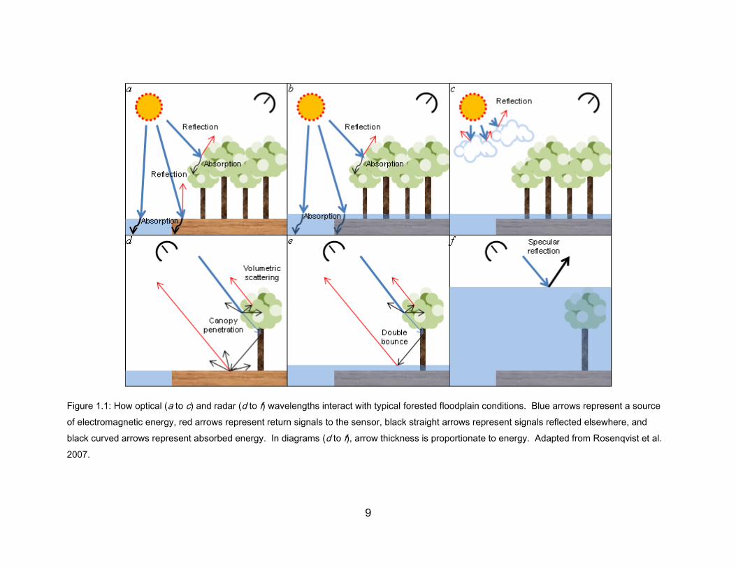
of vegetation and flood extent data for large-scale inventory methods (Figure 1.1,
De Grandi et al. 2000a, Hess et al. 2003, Rosenqvist et al. 2007).
1.3.2 Radar Data
Unlike the passive nature of optical sensors which depend on reflected
solar energy, radar sensors are active, sending a pulse of radiation from the
satellite to the target and then recording the amount reflected (Figure 1.1). The
active nature and comparatively long (microwave) wavelength of radar signals
mean that data can be collected independent of time of day or cloud cover. The
most common radar bands used for tropical wetland mapping are C-band (5.6
cm) and L-band (23.5 cm) (De Grandi et al. 2000a, Costa et al. 2002, Mayaux et
al. 2002, Hess et al. 2003, Hamilton et al. 2007, Durieux et al. 2007). Longer
9
Figure 1.1: How optical (a to c) and radar (d to f) wavelengths interact with typical forested floodplain conditions. Blue arrows represent a source
of electromagnetic energy, red arrows represent return signals to the sensor, black straight arrows represent signals reflected elsewhere, and
black curved arrows represent absorbed energy. In diagrams (d to f), arrow thickness is proportionate to energy. Adapted from Rosenqvist et al.
2007.
10
wavelengths penetrate deeper into vegetation canopies, but lose sensitivity to
smaller biophysical vegetation characteristics such as leaf distribution, density,
orientation, canopy structure, and plant biomass (Silva et al. 2008). It is
important to note that radar systems are side-looking, the inclination of which
also affects the amount of energy that is returned as well as specularly reflected
(Figure 1.1). Radar pulses can be returned to the sensor via the volumetric
backscattering characteristic of vegetation canopies, and via the corner or di-
hedral reflection characteristic of urban areas and flooded vegetation, where
many surfaces occur at perpendicular angles (Figure 1.1). The longer
wavelengths of radar data, compared to optical data, cannot penetrate water, so
they are not sensitive to submerged vegetation, but can be sensitive to flooded
vegetation stands.
C-band radar provides information about forest canopy structure via
volume backscattering since it is often completely attenuated there (De Grandi et
al. 2000, Mayaux et al. 2002), but also shows strong di-hedral reflectance from
flooded herbaceous vegetation (Costa et al. 2002, Mayaux et al. 2002). The
longer wavelength of L-band radar almost completely penetrates forest canopy
vegetation and reflects a portion back to the sensor via corner-bouncing between
the flooded surface and tree trunks (Silva et al. 2008). For this reason, L-band
radar has long been used to reliably estimate the flood extent of flooded forest,
11
but is less successful at mapping wetland vegetation with less biomass such as
shrub and herbaceous classes (e.g., Hess et al. 1995, Hess et al. 2003).
However, radar data are increasingly considered a critical component of tropical
wetland classifications due to their ability to penetrate cloud cover and their
sensitivity to the presence of standing water beneath vegetation (Rosenqvist et
al. 2007).
The latest generation of radar platforms provides an additional dimension
of information with the ability to send and receive radar signals in different
polarizations (e.g., RADARSAT-2, ALOS/PALSAR). Polarized electromagnetic
radiation vibrates linearly. Traditionally, radar sensors have only recorded signals
in same- or co-polarized wavelengths such as HH (sending and receiving a
horizontally polarized wavelength, e.g., JERS-1/SAR) or VV (sending and
receiving a vertically polarized wavelength, e.g., RADARSAT-1). The most
advanced radar satellites now enable cross- (e.g., HV), dual- (e.g., HH+HV) and
quad-polarization (HH+HV+VV+VH) techniques for much more complex
vegetation structure analyses. Plant density, distribution, orientation, foliage
shape, dielectric constant, canopy height, and soil moisture are all characteristics
that radar still has the potential to capture in this way (Costa 2004). However,
unlike optical spectral signatures, polarization signatures can be the same for two
different scatterers (CCRS 2007).
12
1.3.3 Ancillary Data
Using only satellite imagery to classify tropical wetlands can be
problematic (Sader et al. 1995). Tropical floodplain wetlands cannot necessarily
be defined by their vegetation or flooding extent in a single satellite image, since
wetland vegetation and flood extent are seasonally variable. Comparing or
compositing multi-temporal imagery is one solution to this problem, but caveats
remain. Coarse-resolution datasets provide regularity and homogeneity of
acquisition dates at the expense of losing small features, which invariably
includes most wetlands (Mayaux et al. 2004, Vancutsem et al. 2009). Fine-
resolution datasets provide the necessary spatial and spectral detail to identify
and classify wetlands, but suffer from the heterogeneity of acquisition dates and
image availability (Vancutsem et al. 2009). Adding complimentary datasets can
be a logical solution to the problem of temporally inconsistent imagery and rapid
wetland mapping. Many wetlands are restricted to certain soils, slopes, and
topography as well as to relationships with other landscape features that are not
directly evident in satellite imagery (Sader et al. 1995). In this way, ancillary data
add to the convergence of evidence needed for accurate wetland detection and
classification (Sader et al. 1995).
Ancillary data are often added as a thematic layer in a Geographic
Information System (GIS) for analysis, and typically improve wetland
13
classification provided that the data are co-registered accurately (Ozesmi and
Bauer 2002). Common themes include soil types, elevation and other wetland
maps (Ozesmi and Bauer 2002). In two of the earliest examples of multiple
dataset analysis in a GIS, Bolstad and Lillesand (1992) and Sader et al. (1995)
both found soil and elevation data aided in accurately classifying wetlands.
Overall accuracy improved from 69% to 83% when soil texture and topographic
position were considered. For floodplain wetland classification, Digital Elevation
Models (DEMs) are particularly useful because they can readily highlight the low
slope and elevation characteristics of floodplain geomorphology (Mertes 2002).
Hamilton et al. (2006) combined the imagery from LANDSAT-7/ETM+ and JERS-
1/SAR over a reach of the Madre de Dios River in the Peruvian Amazon with a
DEM. The DEM was used in the initial step of their analysis to distinguish
floodplain from nonfloodplain areas (Hamilton et al. 2007). This study employed
a rule-based approach similar to Bolstad and Lillesand (1992) and Sader et al.
(1995) which, being a knowledge-based method of analysis, is served well by
ancillary data (Daniels 2006). Although ancillary data are useful for improving the
accuracy and detail of wetland classification, ultimately it is the responsibility of
the analyst to interpret and classify such data for practical use.
14
1.3.4 Image Analysis
Conceptually, pixel-based classification methods lack an intrinsic
relationship to the boundaries of ecosystems since the boundaries of pixels are
imposed during data processing (Hess et al. 2003). Pixel-based classification
can also be problematic for ecological applications because the low statistical
separability of classes results in either low accuracy or the use of very general
classes (Lobo 1997). An object-oriented approach, in contrast, segments an
image into more or less homogeneous regions (objects) that are then classified
based on aggregate statistics of the pixels within the object.
Additionally, some software packages can semi-automatically, and thus
rapidly, integrate several datasets of varying spatial and spectral resolutions into
objects that can then be classified based on shape, texture, area, context, and
information from other hierarchical object layers (e.g., Hamilton et al. 2007,
Durieux et al. 2007). The object-oriented approach is proving to be an effective
tool for improving the accuracy of and discriminating between wetland classes
(Costa et al. 2002, Hess et al. 2003, Hamilton et al. 2007, Durieux et al. 2007). A
distinct advantage of the object-oriented approach is that both descriptive and
strategic information used for image segmentation and wetland classification are
explicitly represented and changeable in the decision tree (or process tree),
15
allowing incremental improvement and new datasets and techniques to be added
when applying or adapting a particular analysis elsewhere.
The concept of image segmentation as applied in an object-oriented
approach is also very useful when analyzing radar data in particular. Radar data
always include spurious data values known as speckle or noise. In a traditional
pixel-based classifier these values would be classified differently from their
neighbours despite the context of the situation (Oliver and Quegan 1998). An
object-oriented approach builds objects from a single pixel and then, based on
user-defined rules of homogeneity, grows and merges the single pixel with
neighbours in an iterative process (Oliver and Quegan 1998). This technique
alleviates the speckle issue of radar data and has been widely adopted for radar-
based tropical wetland classification (Costa et al. 2002, Hess et al. 2003, Costa
and Telmer 2007).
1.3.5 Tropical Floodplain Wetland Classification
For the purposes of large-scale hydrology and biogeochemistry research,
especially for methane emissions, satellite radar imagery is sufficient for mapping
functional wetland types. This is because hydrological models do not yet
incorporate wetland functional vegetation classes, and because methane
emissions from tropical wetlands are dependent on three basic floodplain
environments with distinct differences in canopy structure (open water, emergent
16
herbaceous vegetation, and flooded forest) (Devol et al. 1990). Each of these
environments involves different rates of water retention and evaporation, as well
as production, oxidation and pathways of methane to the atmosphere. There
remains considerable variability of methane release from each of these
environments, but greater uncertainty lies in estimating the changing extent of
these environments during the flooding cycles of tropical basins (Melack et al.
2004). The wetland classification scheme of Hess et al. (2003) successfully
followed this approach and has since been used to improve the estimates of
carbon dioxide degassing from the Amazon River (Richey et al. 2002) as well as
to estimate the regional methane emissions from the Amazon basin (Melack et
al. 2004).
Tropical floodplain wetland maps motivated by biodiversity and
conservation concerns also benefit from a physiognomic-hydrologic classification
scheme since such environments also provide information regarding fish habitat
and fisheries management (Hess et al. 2003). The Ramsar Convention on
Wetlands, an intergovernmental treaty meant to provide a framework for national
and international cooperation towards the wise use and conservation of wetlands,
also promotes remote sensing as a key tool for establishing national wetland
inventories and monitoring programs to measure and achieve its goals
(Rosenqvist et al. 2007). However, as radar data are generally incapable of
17
providing species-specific information, the addition of optical data provides more
vegetation-based classifications that are necessary to distinguish important
tropical wetland classes such as Raphia spp., for example (Hess et al. 2003,
Hamilton et al. 2007). Wetland classification, regardless of thematic detail, must
also include some measure of accuracy relative to ground conditions to be
useful.
1.3.6 Accuracy Assessment
Map accuracy is the degree of correspondence between classification and
reality on the ground (Congalton and Green 2009). It is determined by
comparing the map of interest against other maps, imagery or, traditionally,
observations in the field. The latter method is called ground-truthing, and it is the
only true method of accuracy assessment for maps based on remotely sensed
data. However, the time, finances and logistics of conducting field campaigns for
large scale map verification—especially maps with a temporal element—can
make it an impractical method of accuracy assessment (Mayaux et al. 2002). An
effective alternative adopted in large-scale landcover studies in both the Amazon
and Congo basins used videography combined with GPS during low-altitude
flights across the area of interest as validation (De Grandi et al. 2000, Hess et al.
2003). This approach remains out of the financial realm of most map producers,
however. Consequently, comparing one map to another map or type of imagery
18
is the most common method of large-scale assessments (De Grandi et al. 2000,
Mayaux et al. 2002, Durieux et al. 2007, Congalton and Green 2009).
There are several considerations with this approach: the timing of data collection
for producing each map; the spatial resolution of each map; the minimum
mapping areas of each class in each map; class definitions used in each map;
and lastly, the positional and thematic accuracy of the reference map (Congalton
and Green 2009). If these qualities do not match, or if the accuracy of the
reference map is not acceptable, a quantitative assessment between the maps
will not be useful, and a simpler qualitative, visual comparison between the maps
must suffice (Congalton and Green 2009).
If these qualities match and if the accuracy of the reference map is
acceptable, then a quantitative assessment can be performed. An error matrix
(also known as a confusion matrix or contingency table) is the most common and
useful method of comparing the level of correspondence between thematic maps
(Congalton and Green 2009). An error matrix displays not only the number of
mapping units (e.g., pixels, pixel groups, or polygons) from each class of the
producer’s map (in rows) correctly classified according to the classes of the
reference map (in columns), but also how misclassified mapping units were
classified instead (e.g., see Table 3.1). Therefore, an error matrix yields several
measures of accuracy as explained below.
19
Overall accuracy is the sum of all correctly classified mapping units,
regardless of class, divided by the total number of mapping units, and it is usually
expressed as a percentage. There are no established thresholds for acceptable
levels of overall accuracy: ultimately, what qualifies as acceptable is decided by
the user. Large-scale tropical wetland studies show overall accuracies from
approximately 75% with one to four classes to 95% with eight classes (see Case
Studies in section 1.3.7 below).
Producer's accuracy is a measure of the accuracy of a particular
classification scheme and shows what percentage of a particular reference class
was correctly classified (CCRS 2009). Put another way, producer’s accuracy is a
measure of omission, excluding a mapping unit (pixel or object) from the category
to which it truly belongs. Producer’s accuracy is calculated by dividing the
number of correct mapping units of a given class by the actual number of
mapping units of that class in the reference map (CCRS 2009). Since producer’s
accuracy reflects the success of the producer to replicate a given class of the
reference map, there could be an over-quantification error that could cause
producer’s accuracy to be high for a class. For example, in the field, it may be
found that the given class, while mapped correctly according to the reference
map, is overestimated at the expense of correct classifications elsewhere.
20
Providing user’s accuracy helps to alert this possibility to the map user. User's
accuracy is a measure of the reliability of an output map generated from a
classification scheme, telling the user of the map what percentage of a class
corresponds to the ground-truthed class (CCRS 2009). User’s accuracy is a
measure of classifying a mapping unit User's accuracy is calculated by dividing
the number of correct mapping units of a given class by the total number of
mapping units assigned to that class (CCRS 2009). It reflects the success of
properly quantifying and locating the mapping units of a given class.
Another statistic widely used to determine the robustness of a
classification is the Kappa Index of Agreement (KIA, also known as the Kappa or
Khat statistic) (Congalton and Green 2009). It is given by subtracting the
proportion of randomly, correctly classified mapping units (pr) from the proportion
of correctly classified mapping units (pc), divided by the difference between 1 (a
perfect classification) and the proportion of randomly, correctly classified
mapping units (pr) (i.e., [(pc) - (pr)] / [1 - (pr)]). It can be interpreted as the
proportion of correctly classified units beyond what could be explained by
randomly labeling mapping units. Despite its wide use, the KIA confounds
quantification and location error (Pontius Jr. 2000). It also does not penalize for
large quantification errors or reward for accurate quantification (Pontius Jr. 2000).
21
Therefore, the KIA is not a perfect statistical descriptor and its weaknesses must
be acknowledged in its interpretation.
Generally, it has been proposed that a KIA greater than 0.80 indicates
strong agreement; a KIA between 0.40 and 0.80 indicates moderate agreement;
and a KIA less than 0.40 indicates poor agreement (Landis and Koch 1977).
However, when referring to and interpreting these thresholds one must also
consider the quality of the reference data. Although no KIA has been reported in
regional studies of the central Congo and Amazon basins, other means of
accuracy have been employed to interpret the accuracy of these maps.
1.3.7 Case Studies: the Central Congo and Amazon River Basin Floodplains
The most studied wetlands of the Congo River basin lie in the cuvette
centrale congolaise, its vast, well-weathered central floodplain. The wetlands of
the central Congo basin were first mapped by White (1983) who took 15 years to
compile national vegetation maps, consult local experts, and produce his
continent-wide vegetation map based on physiognomy and floristics. White’s
swamp forest, the single wetland class of his exhaustive vegetation map of the
continent, is composed of herbaceous swamp, aquatic vegetation, edaphic
grassland, and riparian forest descriptions (White 1983). Although White’s map
is spatially simple, it contains considerable description of the swamp forest class.
22
However, this method is not appropriate for developing a consistent method of
wetland inventories and updates needed for this rapidly developing region.
The first satellite-produced vegetation maps of the region focused on establishing
a baseline for forest cover in the basin. The spatial (1 km) and spectral
resolution (4 bands visible, 2 bands infrared) of the optical composite imagery
(NOAA/AVHRR) used in these studies was only able to distinguish between
disturbed and undisturbed forest types, and overestimated forest cover by up to
20% due to the large spatial resolution (Laporte et al. 1995, Laporte et al. 1998,
Mayaux et al. 1999a). Separating swamp forest from the tropical forest class
with remotely sensed imagery was not possible until studies began to include
radar imagery.
A single C-band radar dataset (ERS-1/SAR) of 100 m spatial resolution
was used by De Grandi et al. (2000a) to distinguish lowland rain forest from
swamp forest across the entire central basin, and Mayaux et al. (2000)
incorporated the same dataset with optical datasets of larger resolution to make
the same distinction in addition to other nonwetland classes. The C-band dataset
enabled discrimination between lowland and swamp forest based on the texture,
or variability, of the backscatter response over each type of canopy (Figure 1.2,
De Grandi et al. 2000a, Mayaux et al. 2000). The difference in radar texture was
verified using aerial videography, which showed that the lowland rain forest
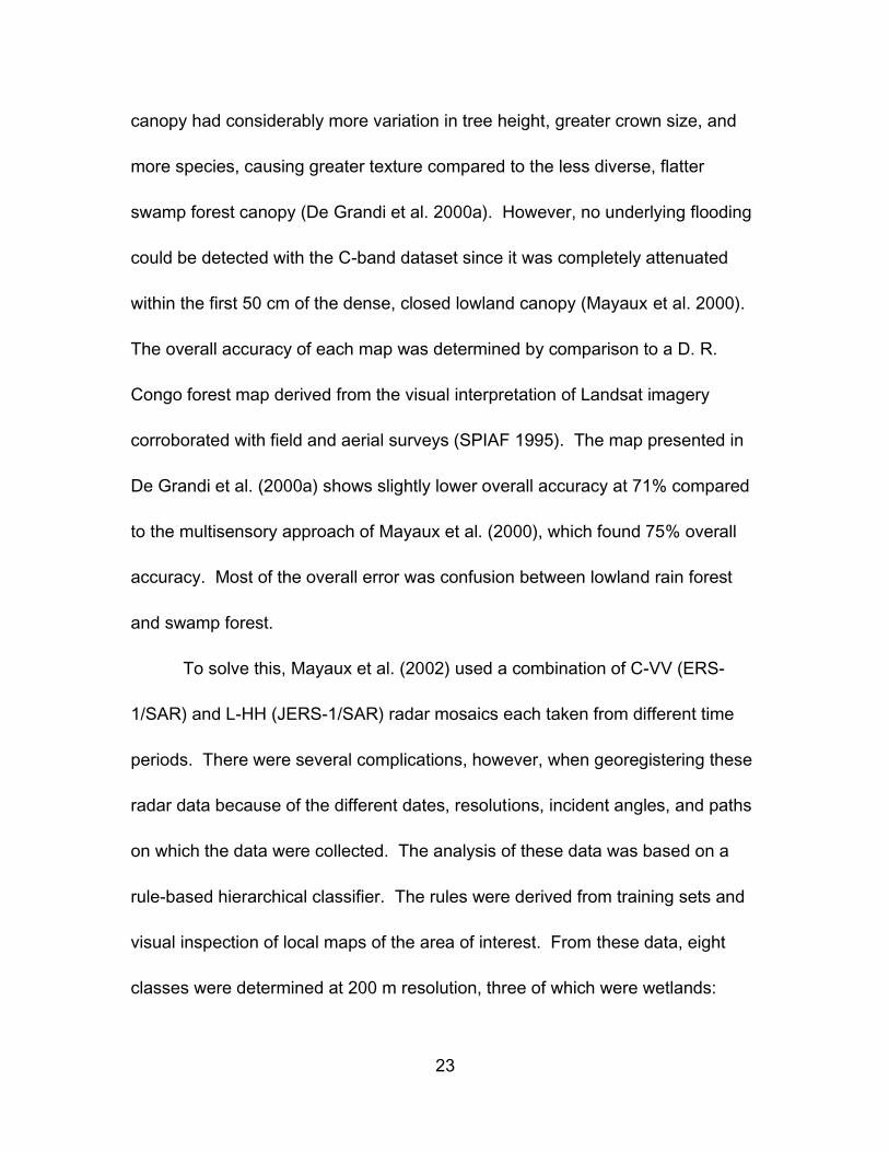
23
canopy had considerably more variation in tree height, greater crown size, and
more species, causing greater texture compared to the less diverse, flatter
swamp forest canopy (De Grandi et al. 2000a). However, no underlying flooding
could be detected with the C-band dataset since it was completely attenuated
within the first 50 cm of the dense, closed lowland canopy (Mayaux et al. 2000).
The overall accuracy of each map was determined by comparison to a D. R.
Congo forest map derived from the visual interpretation of Landsat imagery
corroborated with field and aerial surveys (SPIAF 1995). The map presented in
De Grandi et al. (2000a) shows slightly lower overall accuracy at 71% compared
to the multisensory approach of Mayaux et al. (2000), which found 75% overall
accuracy. Most of the overall error was confusion between lowland rain forest
and swamp forest.
To solve this, Mayaux et al. (2002) used a combination of C-VV (ERS-
1/SAR) and L-HH (JERS-1/SAR) radar mosaics each taken from different time
periods. There were several complications, however, when georegistering these
radar data because of the different dates, resolutions, incident angles, and paths
on which the data were collected. The analysis of these data was based on a
rule-based hierarchical classifier. The rules were derived from training sets and
visual inspection of local maps of the area of interest. From these data, eight
classes were determined at 200 m resolution, three of which were wetlands:
24
Figure 1.2: Aerial videography snapshots of swamp forest (above) and upland, or terra firme,
forest (below) in the central Congo basin. From De Grandi et al. 2000a.
25
permanently flooded forest, periodically flooded forest, and swamp grassland. In
addition to the added wetland class, the accuracy for this map was slightly higher
than that of De Grandi et al. (2000a) and Mayaux et al. (2000) at 76% when
compared to SPIAF (1995). Most of the error was the result of the enhanced
wetland sensitivity of radar in comparison to the optical data used to produce
SPIAF (1995), so 76% is likely an underestimate of the accuracy of the map.
However, both the C-VV and L-HH data were unable to identify strips of
secondary forest along river networks, whereas this forest type is easily
discernable using optical imagery (Mayaux et al. 2002).
The most recent remote sensing of Congo vegetation used daily optical
composites (SPOT/VGT) from the year 2000 at 1 km resolution to produce a new
vegetation map of the D. R. Congo (Vancutsem et al. 2009). Of the six classes
defined, two wetland classes were described: (1) edaphic forest and (2) aquatic
grassland and swamp grassland. These classes constitute the smallest area of
the landcover classes mapped. When experimenting with aggregated classes,
Vancutsem et al. (2009) found that aquatic vegetation was responsible for most
of the overall error with 56% underestimation compared to a reference map
based on 30 m optical (LANDSAT) data (further detail regarding this dataset--
Africover--is given in Methods below). Most of this inaccuracy was the result of
the large resolution of the composites compared to the high resolution of the
26
reference map, which was able to identify typically small and linear wetland
features (Vancutsem et al. 2009). This result of underestimating wetlands is
similar to that found in Mayaux et al. (2004), which also used 1 km optical
composites (NOAA/AVHRR). Finer spatial resolution than 1 km is necessary,
therefore, to accurately determine wetland quantities for regional tropical
floodplain wetlands. A study that addresses the issue of temporal and spatial
resolution with an explicit focus on tropical floodplain wetlands comes from a
study of the central Amazon.
Hess et al. (2003) provide an exemplary application of radar imagery for
classifying tropical floodplain wetlands at a regional scale. Hess et al. (2003)
were able to distinguish between wetland and nonwetland classes over the
central basin of the Amazon River with 95% accuracy using two L-HH mosaics at
100 m resolution taken at high- and low-water conditions in the basin. The
classification scheme was designed to improve regional hydrologic parameters
(Sahagian and Melack 1998), carbon dioxide and methane emission estimates
(Richey et al. 2002, Rosenqvist et al. 2002a), as well as fishery management,
since many fish species depend on the flooded forests for nutrition or organic
matter from floodplain algae (Forsberg et al. 1993). The eight wetland classes
mapped include water, nonflooded bare or herbaceous, flooded herbaceous,
nonflooded shrub, flooded shrub, flooded woodland, nonflooded forest, and
27
flooded forest. It was concluded that although L-HH is the best single-band
sensor for mapping wetlands in the central Amazon basin, the backscatter from
the most common nonwetland cover (nonflooded forest) overlaps with forest and
aquatic macrophyte cover and serves as a major source of confusion for
traditional, pixel-based classification methods.
These studies illustrate that coarse-resolution (> 1 km) though frequently
collected optical imagery alone is not capable of reliably determining flooded
vegetation classes, and suggest radar imagery as a primary source of flooded
vegetation extent in tropical floodplain environments.
28
2. Approach, Study Area and Methods
2.1 Approach
Previous work demonstrates that radar imagery is useful for mapping
several kinds of flooded vegetation in the tropics (De Grandi et al. 2000a,
Mayaux et al. 2002, Hess et al. 2003, Rosenqvist et al. 2007). Indeed, Hess et
al. (2003) was remarkably successful mapping the floodplain wetlands of the
central Amazon basin using only two L-HH radar mosaics.
Therefore, to achieve the objective of a rapid, regional-scale method of
tropical wetland classification, two L-HH radar datasets from the JERS-1/SAR
GRFM Africa project were selected as the primary source of wetland information.
Given the consistent confusion of non-floodplain forest with floodplain forest
classes in previous radar floodplain wetland studies of the central Congo and
Amazon basins (De Grandi et al. 2000a, Mayaux et al. 2002, Hess et al. 2003),
and given the improvement that topographic information provides (Ozesmi and
Bauer 2002, Hamilton et al. 2007), the addition of elevation data (HydroSHEDS
DEM) and elevation derivatives (slope, HydroSHEDS Rivers, SRTM Water
Bodies, for details see section 2.3.1) have also been selected as sources of
wetland information. The rapid and transparent integration and analysis of these
datasets is possible with an object-oriented approach (e.g., Hess et al. 2003,
Hamilton et al. 2007, Durieux et al. 2007).
29
To address the first research question, appropriate classes for
hydrologists, biogeochemists, and conservationists will be achieved by mapping
similar classes to Hess et al. (2003). To adapt the classifier of Hess et al. (2003)
to the varied hydrological conditions captured in the radar imagery of the Congo,
the flooded and nonflooded hydrologic states of the vegetation classes must be
eliminated, simplifying the classifier to 7 classes from 13. This simplification
removes the requirement of an area to transition from nonflooded to flooded from
the low-water to high-water mosaics, and instead indicates that an area was
flooded in one or the other or both (see Data Analysis and Figure 2.8 below for
more detail). The addition of topographic datasets also helps to distinguish
classes and improve accuracy.
To address the third research question of reaching the best compromise
between rapid analysis, thematic detail and accuracy, three maps of decreasing
thematic detail of 7, 5 and 3 wetland classes are compared to similarly
reclassified reference maps in order to determine the effect of a reduced number
of classes on different measures of accuracy.
The study area, datasets, dataset preparation, analysis, and accuracy
assessment are described in further detail below.
30
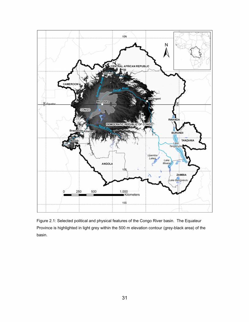
2.2 Study Area
The Equateur Province is an administrative area of the D. R. Congo
located in the centre of the 500 m elevation contour of the Congo River basin
(Figure 2.1). It is approximately 100,000 km2 in size and is representative of
many wetland types. As a part of the central basin, Equateur has been included
in previous wetland descriptions and remote sensing products (Hughes et al.
1992, De Grandi et al. 2000a, Mayaux et al. 2000, Mayaux et al. 2002). These
qualities make it an excellent test area for a method of wetland delineation,
classification, and validation in this otherwise little studied basin.
2.2.1 Physical Setting
As its name implies, Equateur straddles the equator and extends from
approximately 2°N to 2°S and from 16°E to 21°E. Equateur experiences 1800-
2400 mm of rainfall per year (Runge 2007) with mean annual temperatures of 25
to 27°C that change little seasonally (Bultot 1971).
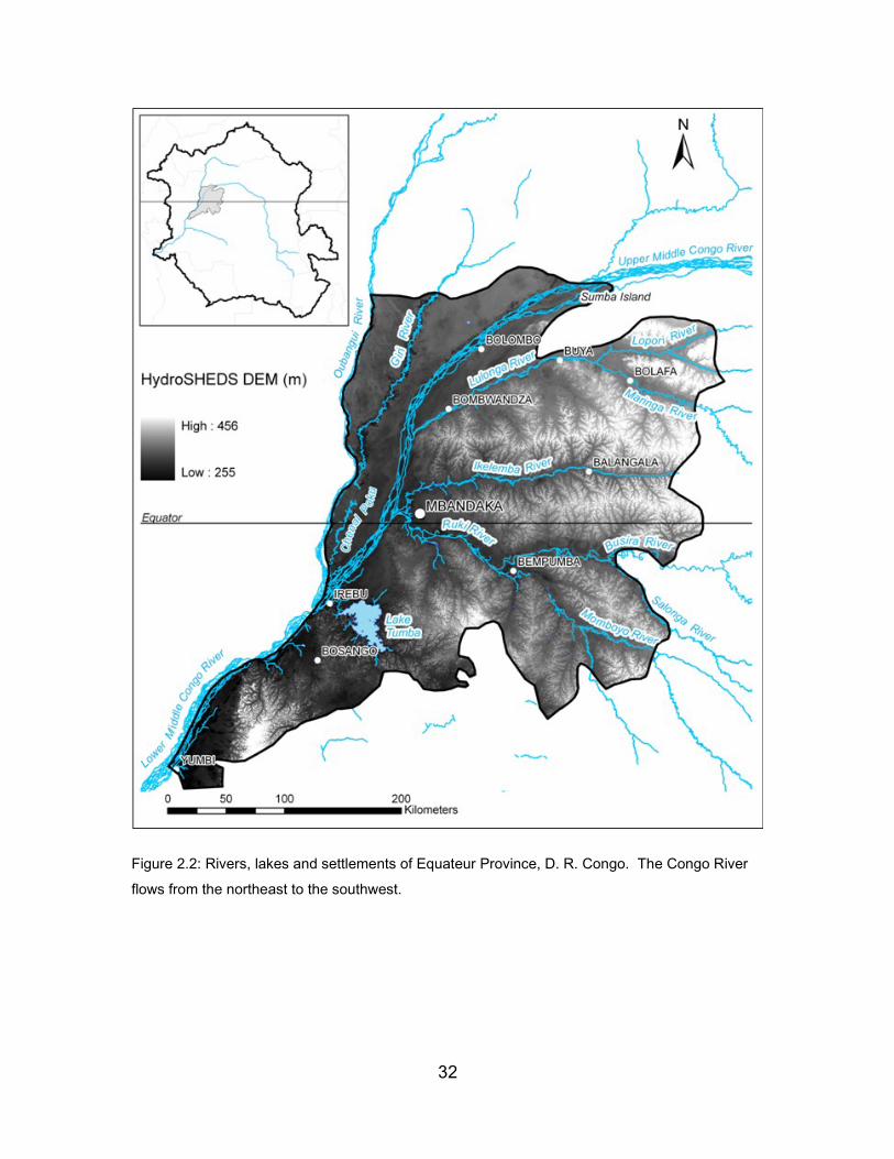
The portion of the Congo River that passes through this region is known
as the Middle Congo, and is characterized by very low slope (1/15,000) and slow
flow, with practically lacustrine conditions surrounding the islands of this
approximately 15 km-wide, anastomosing reach (Hughes et al. 1992, Figure 2.2).
The Congo River flows from Sumba Island in the northeast to a small town called
Yumbi in the southwest of Equateur (Figure 2.2). At Mbandaka, the Congo River
31
Figure 2.1: Selected political and physical features of the Congo River basin. The Equateur
Province is highlighted in light grey within the 500 m elevation contour (grey-black area) of the
basin.
32
Figure 2.2: Rivers, lakes and settlements of Equateur Province, D. R. Congo. The Congo River
flows from the northeast to the southwest.
33
has an average annual stage rise of 1.8 m, which is much less than the 15 m
found at Manaus on the Rio Negro of the Amazon (Campbell 2005).
The confluence of the largest tributary of the Congo River, the Oubangui,
as well as the Giri, Lulonga, Ikelemba, and Ruki Rivers occur in Equateur (Figure
2.2). Since the Congo River crosses the equator twice with large tributaries
flanking on either side, Equateur tributaries show both uni-modal and bi-modal
discharge patterns depending on their size and location relative to the equator.
The right-bank tributaries (the Oubangui and Giri Rivers) both show unimodal
hydrographs (Runge 2007). The Oubangui has the largest floodwave in the
basin, rising up to 8 m in October and November with a stage low in March and
April (Runge and Nguimalet 2005). The left-bank tributaries (Lulonga, Ikelemba
and Ruki Rivers) of this region share bimodal discharge patterns, with peaks
occurring from November to January and a lesser peak in March to May
(Rosenqvist and Birkett 2002). Lake Tumba, the second largest lake of the
central basin at approximately 500 km2, lies in the southern portion of Equateur.
The alluvial plains of the middle Congo, Oubangui and Giri are composed
of sands and clays high in organic matter (Campbell 2005). Sands dominate in
the alluvium of the southern tributaries, and in some backwater swamps peat
deposits occur up to 17 m deep (Campbell 2005). The waters of the central
Congo River are black with relatively high dissolved organic matter (5 mg/L)
34
comprising 86% of its total organic carbon load, comparable to the Rio Negro of
the Amazon (Coynel et al. 2005).
2.2.2 Central Congo Floodplain Wetlands
The Middle Congo exhibits extensive wetlands. On the right bank, where
the Oubangui River converges with the Congo, 231,000 ha of flooded forest and
perhaps another 100,000 ha in minor riparian swamps are estimated to occur
(Hughes et al. 1992). The wetlands associated with this river are similar to those
associated with the Congo mainstem, i.e., fringing flooded forest. Behind the
levees of the Oubangui are backwater swamps that are periodically flooded and
can extend up to 35 km from the river (Hughes et al. 1992).
The Giri River drains the area between the Oubangui and the Congo
Rivers, joining with the Oubangui shortly before its confluence with the Congo
River. The Giri is unique in this region for its extensive shrubs and herbaceous
vegetation in its floodplain, in addition to having several channels connecting it
with the Congo River as it meanders between the Oubangui and the Congo
(Hughes et al. 1992). There are approximately 3 million ha of waterlogged
flooded forest area between the Congo, Giri and Oubangui Rivers, forming a
triangle of flooded forest from the confluence of the Congo and Oubangui
approximately 375 km long and 165 km across (Hughes et al. 1992).
35
Of the left bank tributaries, the Ruki and Lulonga Rivers both exhibit
extensive flooded forest at their confluences with the Congo River, along their
lengths and beyond along the convergence of their tributaries: the Momboyo and
Busira of the Ruki River, and the Maringa and Lopori of the Lulonga River. The
largest continuous area of permanently and seasonally flooded forest occurs
along the left bank of the Congo River immediately south of the Ruki, covering
about 5 million ha and surrounding Lake Tumba (Hughes et al. 1992).
2.3 Methods
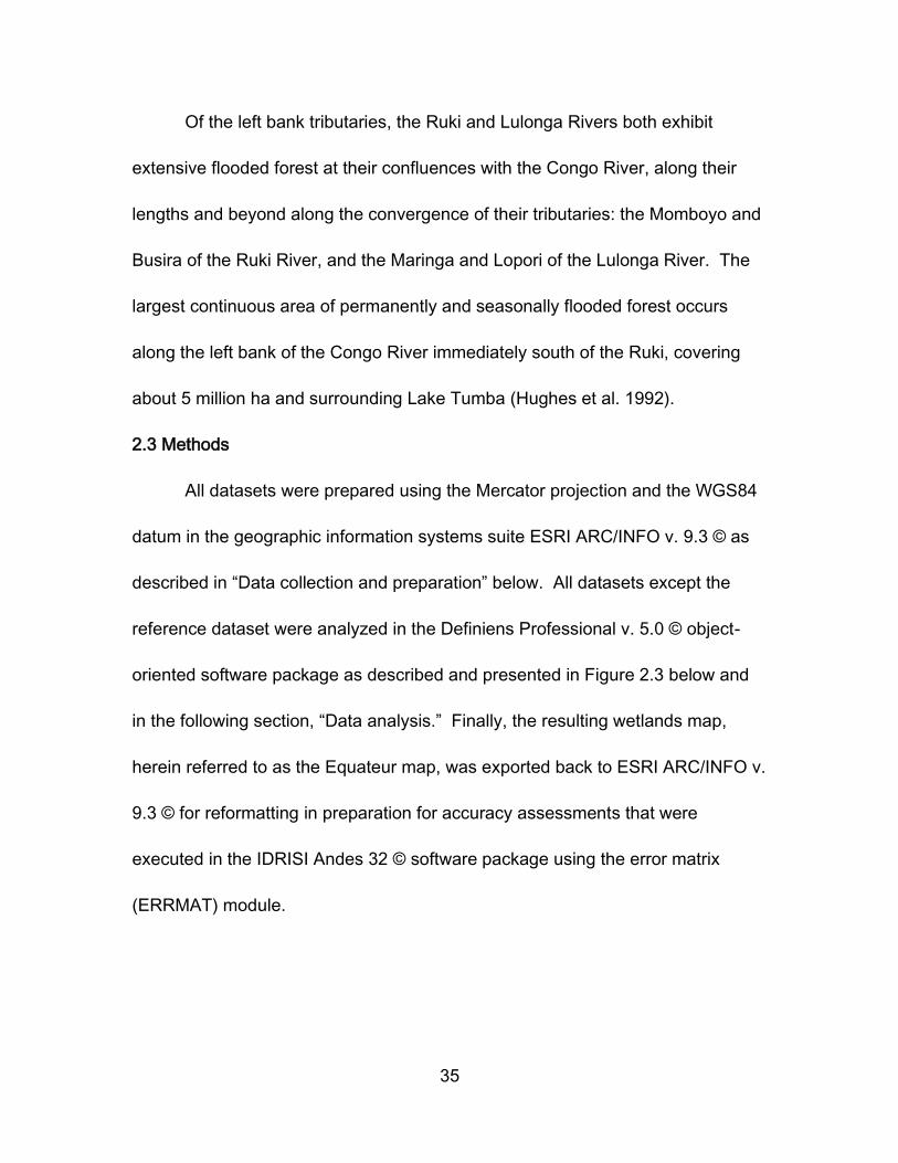
All datasets were prepared using the Mercator projection and the WGS84
datum in the geographic information systems suite ESRI ARC/INFO v. 9.3 © as
described in “Data collection and preparation” below. All datasets except the
reference dataset were analyzed in the Definiens Professional v. 5.0 © object-
oriented software package as described and presented in Figure 2.3 below and
in the following section, “Data analysis.” Finally, the resulting wetlands map,
herein referred to as the Equateur map, was exported back to ESRI ARC/INFO v.
9.3 © for reformatting in preparation for accuracy assessments that were
executed in the IDRISI Andes 32 © software package using the error matrix
(ERRMAT) module.
36
Figure 2.3: A visual overview of each dataset used for the Equateur floodplain wetland delineation and classification.
37
2.3.1 Data Collection and Preparation
2.3.1.1 JERS-1/SAR GRFM Africa Mosaics
Description
The main dataset used in this study for wetland information is from the
Japanese Earth Resources Satellite Synthetic Aperture Radar sensor (JERS-
1/SAR). One of its missions was to establish, for the first time, wall-to-wall
estimates of the world’s tropical forest using L-HH radar at high resolution (12.5
m). Known as the Global Rain Forest Mapping Project (GRFM), the mission
imaged most of the tropics over its lifespan from 1992 to 1998. Several research
centres were charged with developing custom algorithms to produce mosaics of
acceptable radiometric and geometric calibration for particular regions. The
European Commission Joint Research Centre (EC JRC) in Ispra, Italy, was
responsible for the GRFM Africa products, which include two 8-bit mosaics
downsampled to 100 m resolution over most of central Africa.
The two mosaics were compiled from over 3,900 scenes collected
between January and March 1996 and again between October and November
1996. The collection of these scenes was from north to south, east to west, and
it took approximately one month to image the whole basin once (Rosenqvist and
Birkett 2002). While these mosaics are not “snapshots” of the hydrological and
vegetation conditions across the basin, the timing of these collections was
38
designed to coincide with the low- and high-water conditions over the Congo
River basin (Figure 2.3). Using correlations between altimeter readings
(TOPEX/POSEIDON) and historical stage data, Rosenqvist and Birkett (2002)
found that the mosaics represent high-water conditions in the basin well, but the
“low-water” (January to March 1996) mosaic is not representative of actual low-
water conditions in most areas. In Equateur, the Oubangui, Giri and Lulonga
Rivers as well as the lower portion of the Congo River by Yumbi display good
stage separation, whereas the stage separation upstream on the Congo River
and the Ruki River is poor, and river stage separation is very poor (essentially
unchanged between the mosaics) for the Busira and Maringa tributaries
(Rosenqvist and Birkett 2002). Information does not exist on the stage
separation for the Ikelemba River. This prevents the use of these mosaics to
determine the full dynamics of flooding extent across Equateur (Hess et al.
2003). Ultimately, the complex hydrology of the basin makes bi-temporal
mapping insufficient for flood extent studies in the Congo (Rosenqvist and Birkett
2002). Despite these shortcomings, the JERS-1/SAR GRFM Africa mosaics
provide the most extensive and consistent source of radar data over the region,
and the successor to the JERS-1/SAR, the ALOS/PALSAR, is designed to
address this deficiency with new data products that can be incorporated into
future analyses (see Discussion in Chapter 4).
39
Another important property of these data is that the mosaics are not
orthorectified. This can cause geographic displacements in areas of high
elevation, especially over mountainous terrain where the off-nadir angle of radar
signals reflect off of steep slopes causing foreshortening and shadow effects.
With the exception of mountainous areas, Birkett and Rosenqvist (2002)
concluded that the geometric accuracy of the mosaics is still appropriate for
hydrological applications and for use with other datasets. The absolute
geolocation accuracy of the basin is 240 m, which is considered excellent for
such a large area (De Grandi et al. 2000b). The 8-bit, 100 m data are available
free for non-commercial purposes as a set of 15 tiles for each low and high-water
season by request from the EC JRC.
Preparation
The metadata of the JERS-1/SAR GRFM Africa mosaics included the
projection and coordinate information for each tile so that the entire mosaic could
be reconstructed; however, the provided coordinates were not precise enough to
do so. As suggested in the metadata, a manual “sliding” technique was needed
to ensure that there were no gaps between the tiles. The coordinates of each tile
were shifted to match seamlessly, without overlap, to the edges of the centre tile
for both mosaics. The centre tile was chosen as the reference tile because it is
most central to the basin and also happens to be where the majority of wetlands
40
occur. The cumulative error involved with sliding a set of tiles to a single
reference tile is also reduced this way, and maximizes the cumulative error at the
periphery of the basin where wetlands are least likely to occur. Ultimately the
largest shift required was 70 m, or less than a pixel’s distance.
The tiles were then merged to form a single mosaic for the low-water and
also for the high-water conditions. Each mosaic was converted to normalized
radar cross section (RCS) values, that is, from 8-bit digital numbers (DNs) to 32-
bit floating point decibel (dB) values following an equation given in the metadata.
The result is an improvement in scaling upon the 8-bit DNs, making them suitable
for map-making using automatic supervised image classification such as in an
object-oriented approach (De Grandi et al. 2000b).
The mosaics were then georectified to the SRTM Water Bodies dataset
using thirty-six ground control points (GCPs) with at least one point from each tile
(the characteristics of the SRTM Water Bodies dataset is given below). Areas of
high elevation and mountainous terrain were avoided in this step since the
mosaic tiles were not orthorectified and thus GCPs in these areas would affect
the resulting error and transformation significantly. The mosaics were rectified
using a cubic-convolution kernel and a third-order polynomial function. The
residual mean square error was 87 m.
41
To improve computational efficiency and the stability of the image analysis
program, the RCS-transformed data were subsequently converted to fit within an
8-bit range, while retaining the RCS values to one decimal place. The typical
range for L-band radar data is approximately from -20 dB for areas such as
water, to -3 dB for areas such as settlements and flooded forest. Therefore, a
value of 25 was added to the RCS values to convert to positive values, and then
the numbers were multiplied by 10 to preserve one decimal place, and finally the
numbers were truncated to whole numbers to produce unsigned 8-bit data. (e.g.,
using [ RCS + 25 ] * 10 with truncation, the RCS range of the low-water mosaic
was transformed from {(-21.9) – (-1.2)} to {31 – 238}). Finally, the mosaics were
clipped to Equateur’s coverage.
2.3.1.2 HydroSHEDS DEM and Derivatives
Description
The HydroSHEDS project (Hydrological data and maps based on shuttle
Elevation Derivatives at multiple Scales) (Lehner et al. 2006) provides several
types of hydrographic information for regional and global-scale studies based on
the Shuttle Radar Topography Mission (SRTM) Digital Elevation Model (DEM).
The SRTM was flown by the space shuttle Endeavor for eleven days in February
2000. A Shortwave Infrared (SIR) C-band (5.3 cm) sensor imaged the elevation
of the Earth between 60°N and S at 1-arc second (approximately 30 m)
42
resolution. It was a joint project between NASA (National Aeronautics and Space
Administration), NGA (National Geospatial-Intelligence Agency of the U.S.
department of defense), the German Aerospace Centre (DLR) and the Italian
Space Agency (ASI). The SRTM 3-arc second (approximately 90 m) DEM was
originally created by NASA’s Jet Propulsion Lab (JPL) and processed to Digital
Terrain Elevation Data (DTED) standards by NGA. More detail about the mission
is provided in Farr and Kobrick (2000). The HydroSHEDS datasets of interest
derived from the SRTM DEM are the HydroSHEDS DEM and HydroSHEDS
Rivers, which were downloaded free of charge from the USGS SRTM
HydroSHEDS server (http://hydrosheds.cr.usgs.gov/).
The HydroSHEDS DEM combines the advantages of the SRTM-3 and
DTED-1 data because the SRTM-3 data are averaged and reduce radar noise
while the DTED-1 was sampled and more clearly represents shorelines and
waterbodies (Lehner et al. 2006). However, an important artifact of the source
data is its inability to penetrate dense vegetation since the C-band wavelength
cannot penetrate dense canopies such as tropical forest. This causes error in
the height estimation, especially over areas such as the Congo floodplain forest
where canopies can reach or exceed 40 m in height. For technical reasons the
data were shifted 1.5 arc-seconds (approximately 45 m) to the north and east
and each tile’s overlapping right column and row were removed (Lehner et al.
43
2006). The HydroSHEDS Rivers dataset is based on a flow accumulation layer
derived from the DEM data at 15 arc-second (approximately 450 m) resolution
with a threshold of 100 upstream cells (Lehner et al. 2006) (Figure 2.3).
Preparation
Twenty-three tiles were required to cover the basin and were merged into
a single mosaic. The mosaic was then reprojected using cubic-convolution
resampling, shifted 45 m south and west to correct for the displacement in its
production, and, along with the basin’s HydroSHEDS Rivers dataset, clipped
using the Equateur theme (Figure 2.3).
With the HydroSHEDS DEM of Equateur, a slope layer (in degrees) was
produced. The 32-bit floating point dataset was transformed to 8-bit data by
multiplying the result by 10 to preserve a decimal place and by truncating the
number to provide a whole number, changing the range of slope from {0 –
13.9038} to {0 – 139} (Figure 2.3).
Since these datasets are based on the same elevation data as the SRTM
Water Bodies (Lakes) dataset—the georeference dataset—georectification was
not required or performed for the DEM or river network.
44
2.3.1.3 SRTM Water Bodies (Lakes)
Description
The SRTM Water Bodies Dataset (SWBD) was developed as a by-product
of NGA’s editing of the SRTM DEM. Ocean, lake and river shorelines were
identified and delineated from 1 arc-second (approximately 30 m) DTED-2 data
and saved as polygons. An important artifact of these data is the timing of the
acquisition: the world’s waterbodies are delineated as they appeared in February
2000. The accuracy of the dataset is within 20 m in the horizontal and 16 m in
the vertical direction (SWBD 2003). Only lakes greater than 600 m in length and
183 m in width are included. Islands with a medial length greater than 300 m are
included, as are smaller islands if more than 10% of the area exceeds 15 m
above the surrounding water. The dataset used in this study had all river
polygons, which are also part of SWBD, removed previously.
Preparation
The SWBD Lakes dataset was clipped to the Equateur region.
2.3.1.4 Reference Map dataset: FAO Africover
Description
The United Nations Food and Agriculture Organization (FAO) began a
landcover mapping initiative for Africa to improve the natural resource
management of this data-poor region. The FAO Africover project began with
45
countries in east and central Africa with the eventual goal of creating an Africa-
wide, exhaustive, multi-purpose landcover map (Di Gregorio and Jansen 2005).
The maps are derived separately for each country using optical, 30 m
(LANDSAT) imagery as the data source. The imagery is interpreted and digitized
into polygons by local experts according to the UN’s Land Cover Classification
System (LCCS) with the flexibility of custom classes where deemed appropriate.
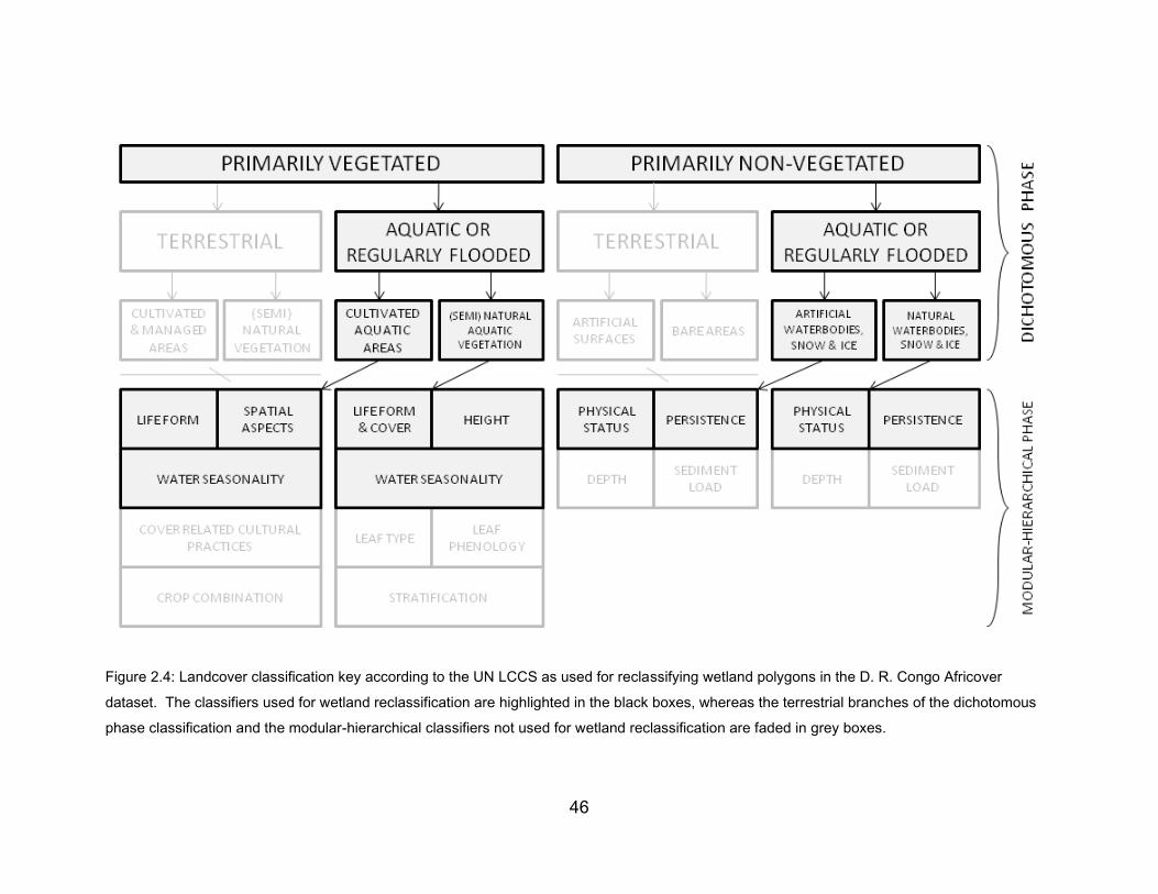
The LCCS proceeds in two phases. The first phase is strictly dichotomous
which sorts a polygon in three steps, producing eight basic classes (Figure 2.4).
The second phase of classification is also hierarchical but the classifiers are
specific to each of the eight basic classes (Figure 2.4). Many classifications are
possible; for the Africover data available for the D. R. Congo, for example, over
80 classes are used, approximately twenty of which could be considered wetland
(i.e., a vegetated area that is flooded for at least 2 months of the year). The
accuracy of the dataset is reported to exceed 60% for the eight primary classes
derived from the first phase of classification, but no accuracy assessment has
been conducted for the classes derived in the second phase of classification (Di
Gregorio and Jansen 2005).
Each polygon has at least one classification. It is possible to have more
than one classification in the case that a feature is too small to be mapped alone
according to the minimum mapping area used. The minimum mapping area
46
Figure 2.4: Landcover classification key according to the UN LCCS as used for reclassifying wetland polygons in the D. R. Congo Africover
dataset. The classifiers used for wetland reclassification are highlighted in the black boxes, whereas the terrestrial branches of the dichotomous
phase classification and the modular-hierarchical classifiers not used for wetland reclassification are faded in grey boxes.
47
(MMA) concept is applied by cartographers when addressing the smallest area
that can be shown on a map (Di Gregorio and Jansen 2005). In Equateur, the
MMA of wetland classes is 34 ha. In the case of two classifications given for a
polygon, one feature dominates the cover of the other within the polygon, and the
second cover still covers at least 20% of the polygon (Di Gregorio and Jansen
2005). In the case of three classifications, the dominant feature approximates
40% cover, while the remaining two features each approximate 30% cover (Di
Gregorio and Jansen 2005). However, no polygons were composed of three
features in the Equateur Province. This mixed mapping unit description allows
some degree of fuzziness or thematic uncertainty to be expressed in the polygon
classification (Di Gregorio and Jansen 2005).
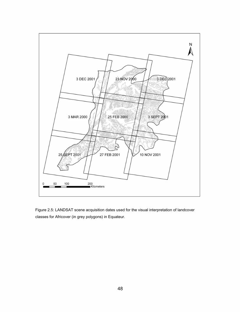
The imagery used for creating the D. R. Congo Africover portion of the
Equateur Province was collected from 2000 to 2001 (Figure 2.5). With no
seasonal or annual consistency between the scenes, interpreting the hydrology
classifier of potential wetland polygons bears a few caveats. Firstly, as the
scenes are not from a single season, the hydrological conditions across Equateur
are not consistent. Secondly, the hydrology classifier has three levels: inundation
for at least 2 months of the year; inundation between 2 and 4 months of the year;
and waterlogged conditions. Since the imagery is not multi-temporal, there is no
way to ascertain the length of time an area has been flooded for. This is in
48
Figure 2.5: LANDSAT scene acquisition dates used for the visual interpretation of landcover
classes for Africover (in grey polygons) in Equateur.
49
addition to the difficulty of determining the extent of flooding under vegetation
canopies using optical imagery. Therefore, it is assumed that the hydrology
classifier was based upon the expert knowledge and interpretation of wetland
vegetation as an expression of flooding characteristics.
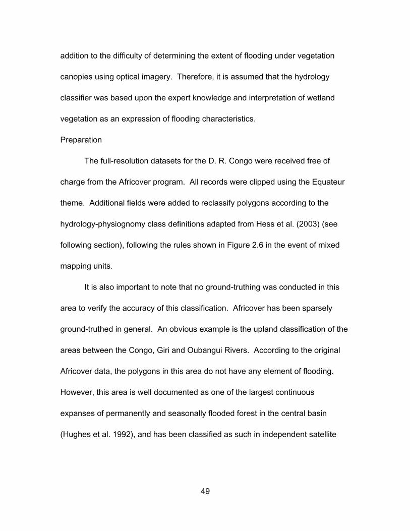
Preparation
The full-resolution datasets for the D. R. Congo were received free of
charge from the Africover program. All records were clipped using the Equateur
theme. Additional fields were added to reclassify polygons according to the
hydrology-physiognomy class definitions adapted from Hess et al. (2003) (see
following section), following the rules shown in Figure 2.6 in the event of mixed
mapping units.
It is also important to note that no ground-truthing was conducted in this
area to verify the accuracy of this classification. Africover has been sparsely
ground-truthed in general. An obvious example is the upland classification of the
areas between the Congo, Giri and Oubangui Rivers. According to the original
Africover data, the polygons in this area do not have any element of flooding.
However, this area is well documented as one of the largest continuous
expanses of permanently and seasonally flooded forest in the central basin
(Hughes et al. 1992), and has been classified as such in independent satellite
50
Figure 2.6: Reclassification rules of Africover mixed mapping units.
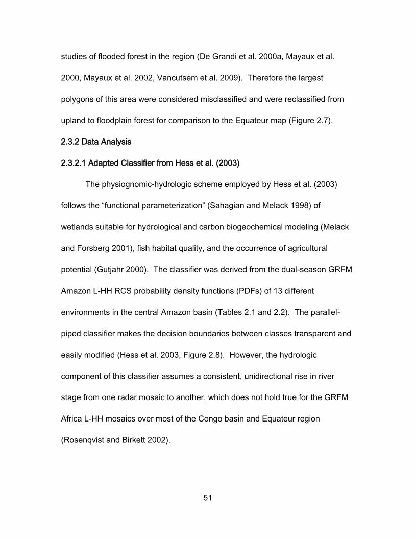
51
studies of flooded forest in the region (De Grandi et al. 2000a, Mayaux et al.
2000, Mayaux et al. 2002, Vancutsem et al. 2009). Therefore the largest
polygons of this area were considered misclassified and were reclassified from
upland to floodplain forest for comparison to the Equateur map (Figure 2.7).
2.3.2 Data Analysis
2.3.2.1 Adapted Classifier from Hess et al. (2003)
The physiognomic-hydrologic scheme employed by Hess et al. (2003)
follows the “functional parameterization” (Sahagian and Melack 1998) of
wetlands suitable for hydrological and carbon biogeochemical modeling (Melack
and Forsberg 2001), fish habitat quality, and the occurrence of agricultural
potential (Gutjahr 2000). The classifier was derived from the dual-season GRFM
Amazon L-HH RCS probability density functions (PDFs) of 13 different
environments in the central Amazon basin (Tables 2.1 and 2.2). The parallel-
piped classifier makes the decision boundaries between classes transparent and
easily modified (Hess et al. 2003, Figure 2.8). However, the hydrologic
component of this classifier assumes a consistent, unidirectional rise in river
stage from one radar mosaic to another, which does not hold true for the GRFM
Africa L-HH mosaics over most of the Congo basin and Equateur region
(Rosenqvist and Birkett 2002).
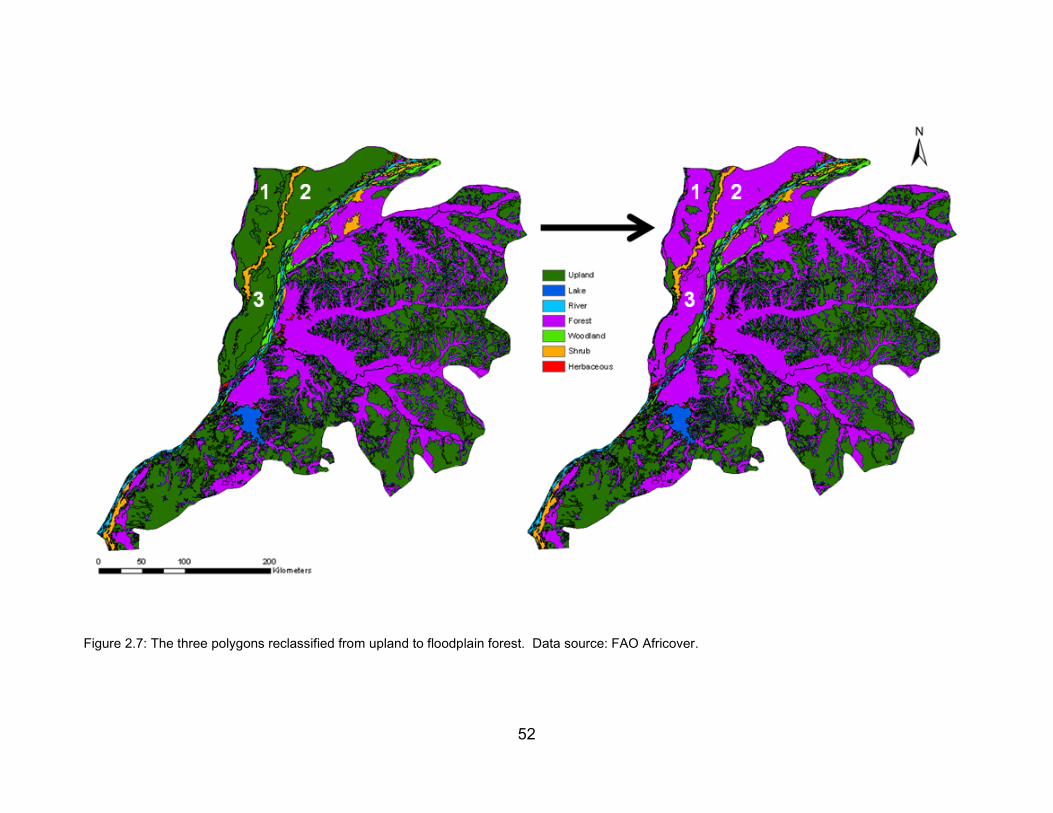
52
Figure 2.7: The three polygons reclassified from upland to floodplain forest. Data source: FAO Africover.
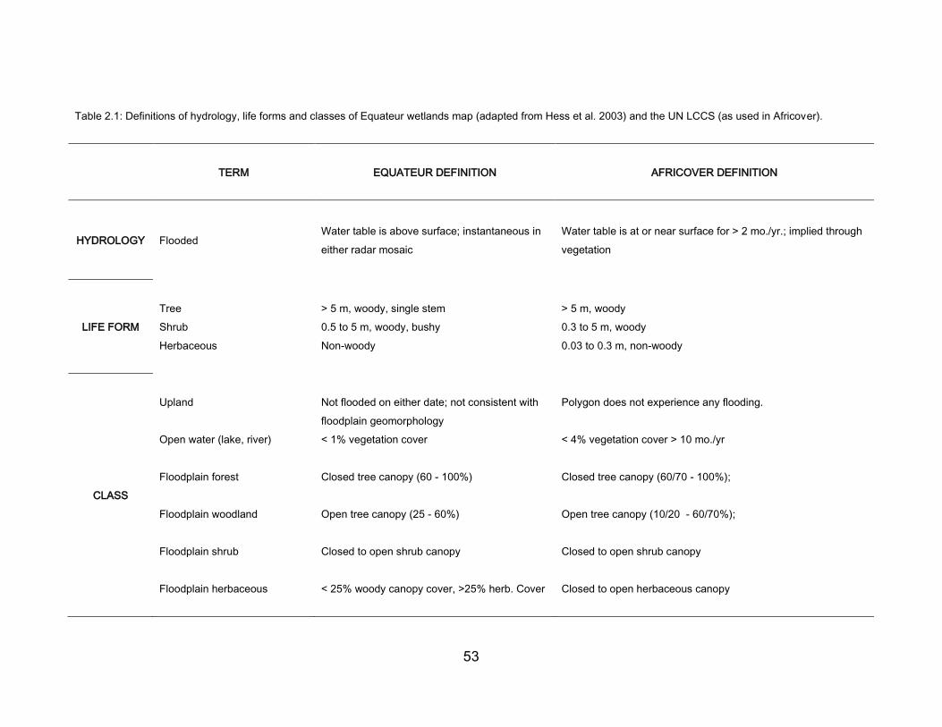
53
Table 2.1: Definitions of hydrology, life forms and classes of Equateur wetlands map (adapted from Hess et al. 2003) and the UN LCCS (as used in Africover).
TERM EQUATEUR DEFINITION AFRICOVER DEFINITION
HYDROLOGY Flooded Water table is above surface; instantaneous in
either radar mosaic
Water table is at or near surface for > 2 mo./yr.; implied through
vegetation
LIFE FORM
Tree > 5 m, woody, single stem > 5 m, woody
Shrub 0.5 to 5 m, woody, bushy 0.3 to 5 m, woody
Herbaceous Non-woody 0.03 to 0.3 m, non-woody
CLASS
Upland Not flooded on either date; not consistent with
floodplain geomorphology
Polygon does not experience any flooding.
Open water (lake, river) < 1% vegetation cover < 4% vegetation cover > 10 mo./yr
Floodplain forest Closed tree canopy (60 - 100%) Closed tree canopy (60/70 - 100%);
Floodplain woodland Open tree canopy (25 - 60%) Open tree canopy (10/20 - 60/70%);
Floodplain shrub Closed to open shrub canopy Closed to open shrub canopy
Floodplain herbaceous < 25% woody canopy cover, >25% herb. Cover Closed to open herbaceous canopy
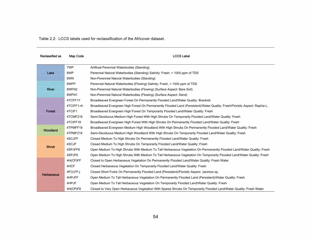
54
Table 2.2: LCCS labels used for reclassification of the Africover dataset.
Reclassified as Map Code LCCS Label
Lake
7WP Artificial Perennial Waterbodies (Standing)
8WP Perennial Natural Waterbodies (Standing) Salinity: Fresh, < 1000 ppm of TDS
8WN Non-Perennial Natural Waterbodies (Standing)
River
8WFP Perennial Natural Waterbodies (Flowing) Salinity: Fresh, < 1000 ppm of TDS
8WFN2 Non-Perennial Natural Waterbodies (Flowing) (Surface Aspect: Bare Soil)
8WFN1 Non-Perennial Natural Waterbodies (Flowing) (Surface Aspect: Sand)
Forest
4TCFF1Y Broadleaved Evergreen Forest On Permanently Flooded Land/Water Quality: Brackish
4TCIFF1-rh Broadleaved Evergreen High Forest On Permanently Flooded Land (Persistent)/Water Quality: Fresh/Floristic Aspect: Raphia L.
4TCIF1 Broadleaved Evergreen High Forest On Temporarily Flooded Land/Water Quality: Fresh
4TCMF218 Semi-Deciduous Medium High Forest With High Shrubs On Temporarily Flooded Land/Water Quality: Fresh
4TCIFF18 Broadleaved Evergreen High Forest With High Shrubs On Permanently Flooded Land/Water Quality: Fresh
Woodland 4TPMFF18 Broadleaved Evergreen Medium High Woodland With High Shrubs On Permanently Flooded Land/Water Quality: Fresh
4TPMF218 Semi-Deciduous Medium High Woodland With High Shrubs On Temporarily Flooded Land/Water Quality: Fresh
Shrub
4SCJFF Closed Medium To High Shrubs On Permanently Flooded Land/Water Quality: Fresh
4SCJF Closed Medium To High Shrubs On Temporarily Flooded Land/Water Quality: Fresh
4SPJFF6 Open Medium To High Shrubs With Medium To Tall Herbaceous Vegetation On Permanently Flooded Land/Water Quality: Fresh
4SPJF6 Open Medium To High Shrubs With Medium To Tall Herbaceous Vegetation On Temporarily Flooded Land/Water Quality: Fresh
Herbaceous
4H(CP)FF Closed to Open Herbaceous Vegetation On Permanently Flooded Land/Water Quality: Fresh Water
4HCF Closed Herbaceous Vegetation On Temporarily Flooded Land/Water Quality: Fresh
4FCLFF-j Closed Short Forbs On Permanently Flooded Land (Persistent)/Floristic Aspect: Jacintus sp.
4HPJFF Open Medium To Tall Herbaceous Vegetation On Permanently Flooded Land (Persistent)/Water Quality: Fresh
4HPJF Open Medium To Tall Herbaceous Vegetation On Temporarily Flooded Land/Water Quality: Fresh
4H(CP)F8 Closed to Very Open Herbaceous Vegetation With Sparse Shrubs On Temporarily Flooded Land/Water Quality: Fresh Water
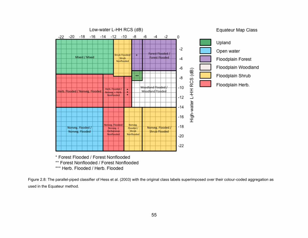
55
Figure 2.8: The parallel-piped classifier of Hess et al. (2003) with the original class labels superimposed over their colour-coded aggregation as
used in the Equateur method.
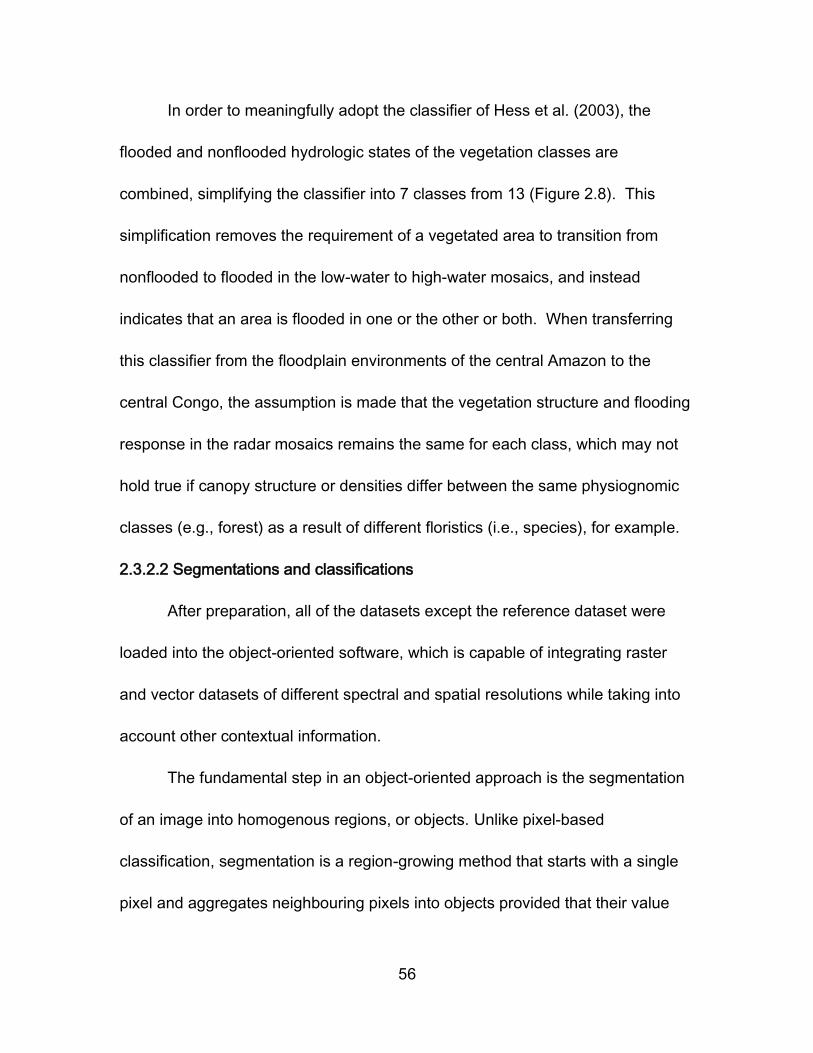
56
In order to meaningfully adopt the classifier of Hess et al. (2003), the
flooded and nonflooded hydrologic states of the vegetation classes are
combined, simplifying the classifier into 7 classes from 13 (Figure 2.8). This
simplification removes the requirement of a vegetated area to transition from
nonflooded to flooded in the low-water to high-water mosaics, and instead
indicates that an area is flooded in one or the other or both. When transferring
this classifier from the floodplain environments of the central Amazon to the
central Congo, the assumption is made that the vegetation structure and flooding
response in the radar mosaics remains the same for each class, which may not
hold true if canopy structure or densities differ between the same physiognomic
classes (e.g., forest) as a result of different floristics (i.e., species), for example.
2.3.2.2 Segmentations and classifications
After preparation, all of the datasets except the reference dataset were
loaded into the object-oriented software, which is capable of integrating raster
and vector datasets of different spectral and spatial resolutions while taking into
account other contextual information.
The fundamental step in an object-oriented approach is the segmentation
of an image into homogenous regions, or objects. Unlike pixel-based
classification, segmentation is a region-growing method that starts with a single
pixel and aggregates neighbouring pixels into objects provided that their value

57
meets the level of homogeneity with their neighbour as specified by the analyst.
It therefore asserts that images are made up of regions and separated by edges
within which a parameter such as the RCS is constant (Oliver and Quegan 1998).
Image segmentation is the most important step of an object-oriented approach
because it produces the fundamental units for classification.
Five segmentation levels were used in this study (consult Figure 2.9 for
details to the following explanations). The first segmentation reduced the number
of objects to a computationally manageable number, as well as distinguished
areas within Equateur from areas outside of Equateur. (The object-oriented
software still considered data imported as “no data” as real data.)
The second segmentation derived upland objects (Figure 2.9). Finding the
appropriate layers, scale and shape factors to segment an area into objects that
reflect landscape units is a process based on inference and trial and error. This
was the most experimental and crucial step of the segmentation processes
because the objects derived at this level were the objects on which the landcover
classifiers acted.
A third segmentation procedure was necessary to delineate open water
objects since radar data, not elevation data, are most sensitive to this feature.
Lake and river objects were further distinguished using the SWBD Lakes dataset
(Figure 2.9).
58
Figure 2.9: Flowchart of the segmentation and classification rules. A legend is highlighted in the
dark grey box.
59
A fourth, growing-region segmentation was applied based on the spectral
difference between unclassified objects (Figure 2.9). This effectively merged
objects with neighbouring objects that are most spectrally similar based on a
user-defined threshold. This extra grow-region segmentation produced a more
continuous and robust river classification based on the open water RCS ranges
in the parallel-piped classifier. Since the grow-region segmentation merged
objects to a level too large for appropriate wetland classification, a fifth and final
segmentation was required for floodplain wetland classification.
The fifth and final segmentation derived floodplain wetland objects. The
fifth segmentation procedure was exactly the same as the third, using only
information from the radar mosaics (Figure 2.9). Only radar information was
required at this level because floodplain wetland objects were classified
according to their mean RCS given by the classifier adapted from Hess et al.
(2003). Since the thresholds are crisp and do not overlap (i.e., not fuzzy), the
order of floodplain wetland object classification was not important, but for
purposes of clarity, were classified in the order of: forest, woodland, shrub, and
lastly, herbaceous vegetation.
After all segmentation and classification steps were completed, a minimum
mapping area of 50 ha for all classes was enforced, following Mayaux et al.
(2002) and Hess et al. (2003) (Figure 2.9).
60
Finally, as there remained considerable confusion between the river and
herbaceous classes at this stage, an additional rule reclassified all smaller,
thinner herbaceous objects as river objects (Figure 2.9).
2.3.2.3 Simplified Wetlands Map and Basic Floodplain Map
Two additional maps were produced from the full, seven-class Equateur
map described above, namely a “simplified” wetlands and a “basic” floodplains
map. Both contain fewer classes as the result of combining classes in strategic
ways.
The simplified wetlands map contains five classes and is based on the a
priori knowledge that dual-season L-HH mosaics are excellent for mapping
flooded trees but have difficulty distinguishing between shrub and herbaceous
vegetation (Hess et al. 2003). Therefore, this map combines the floodplain forest
with the floodplain woodland classes to effectively create a floodplain trees class,
termed “tall vegetation.” The floodplain shrub and herbaceous classes are also
combined to form the “short vegetation” class. The simplified wetlands map
maintains the upland, lake and river classes from the Equateur map without any
change.
The basic floodplain map reduces the number of classes to three to test
the ability of the Equateur method to distinguish the floodplain environment from
upland and open water. It could effectively serve as a wetland mask, for
61
example. A wetlands mask—or, in the case of the tropics, areas that are not a
part of the floodplain,—would include areas that are vegetated but are not
flooded in either radar mosaic nor are consistent with floodplain geomorphology
(upland), as well as areas that are flooded in both mosaics but are not vegetated
(open water). These two conditions translate into the two basic non-wetland
classes of upland and open water and bound the floodplain environment as a
result. This basic classification serves as a benchmark for maximum
correspondence between the Equateur method and the reclassified Africover
map.
2.3.3 Accuracy Assessment
The full Equateur map was exported from the object-oriented software as
a raster file in a Mercator projection with 92.5 m resolution into the GIS in
preparation for accuracy assessment. The Africover data were rasterized to 92.5
m pixels. The Equateur map was shifted east approximately 16.5 m and south
22.1 m to correspond areas of data and no data perfectly with the Africover map,
as required for error matrix generation by the accuracy assessment software. To
achieve this, both maps were masked so that only pixel locations that show data
in both maps are preserved, and those pixels that overlap with “No data” in either
map were eliminated. The class reductions to produce the simplified wetlands
map and basic floodplain map and corresponding reference maps were
62
performed in the GIS with a straightforward reclassification command. All maps
were imported into the accuracy assessment software, where three error
matrices were produced, including measures of overall, producer’s and user’s
accuracy as well as the Kappa Index of Agreement (KIA) between maps.
Quantification, or total area, of each class for each map was also tabulated. The
results for and interpretations of each map and each class are presented below.
63
3. Results and Interpretation
3.1 Full Equateur Wetlands Map
The full Equateur wetlands map includes seven classes: upland, lake,
river, floodplain forest, floodplain woodland, floodplain shrub and floodplain
herbaceous vegetation. It is the most thematically detailed map of the three
produced in this study and is the source of the simplified wetlands map and basic
floodplain map described further below. The Equateur wetlands map and
corresponding Africover map are shown in Figure 3.1. The floodplain woodland
class, however, was discovered to be a misnomer, and is more appropriately
labelled nonflooded forest in contrast with floodplain forest, which is itself more
appropriately labelled flooded forest, for reasons given further below.
The overall accuracy of the full Equateur wetlands map is 47% compared
to the Africover reference map, with a KIA of 28% (Table 3.1). The majority of
the overall map error is confusion between flooded forest and nonflooded forest
pixels. The majority of nonflooded forest commission error (user’s accuracy)
(75%) and omission error (producer’s accuracy) (73%) involves confusion with
Africover’s flooded forest class. Compared to Africover, the flooded forest class
is underestimated by approximately 4,100,000 pixels, whereas nonflooded forest
is overestimated by 4,400,000 pixels: nearly the same amount (Table 3.2).
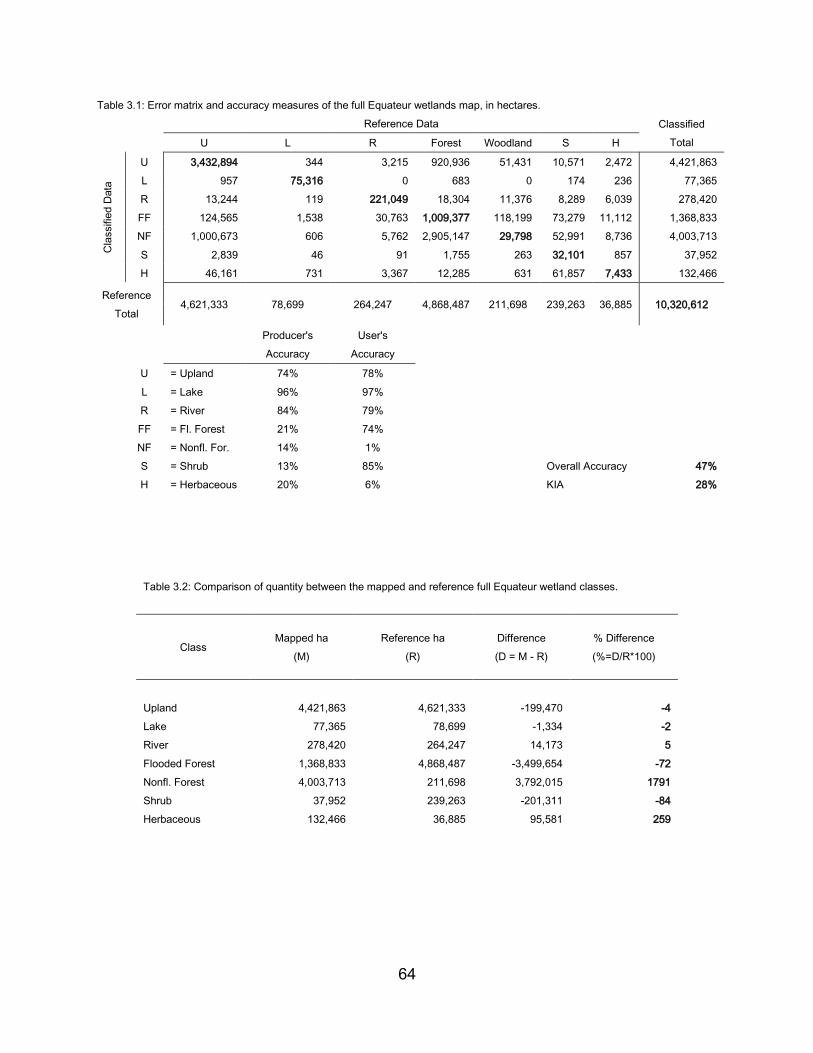
64
Table 3.1: Error matrix and accuracy measures of the full Equateur wetlands map, in hectares.
Reference Data Classified
Total U L R Forest Woodland S H
Cla
ssifie
d D
ata
U 3,432,894 344 3,215 920,936 51,431 10,571 2,472 4,421,863
L 957 75,316 0 683 0 174 236 77,365
R 13,244 119 221,049 18,304 11,376 8,289 6,039 278,420
FF 124,565 1,538 30,763 1,009,377 118,199 73,279 11,112 1,368,833
NF 1,000,673 606 5,762 2,905,147 29,798 52,991 8,736 4,003,713
S 2,839 46 91 1,755 263 32,101 857 37,952
H 46,161 731 3,367 12,285 631 61,857 7,433 132,466
Reference
Total 4,621,333 78,699 264,247 4,868,487 211,698 239,263 36,885 10,320,612
Producer's
Accuracy
User's
Accuracy
U = Upland 74% 78%
L = Lake 96% 97%
R = River 84% 79%
FF = Fl. Forest 21% 74%
NF = Nonfl. For. 14% 1%
S = Shrub 13% 85% Overall Accuracy 47%
H = Herbaceous 20% 6% KIA 28%
Table 3.2: Comparison of quantity between the mapped and reference full Equateur wetland classes.
Class Mapped ha
(M)
Reference ha
(R)
Difference
(D = M - R)
% Difference
(%=D/R*100)
Upland 4,421,863 4,621,333 -199,470 -4
Lake 77,365 78,699 -1,334 -2
River 278,420 264,247 14,173 5
Flooded Forest 1,368,833 4,868,487 -3,499,654 -72
Nonfl. Forest 4,003,713 211,698 3,792,015 1791
Shrub 37,952 239,263 -201,311 -84
Herbaceous 132,466 36,885 95,581 259
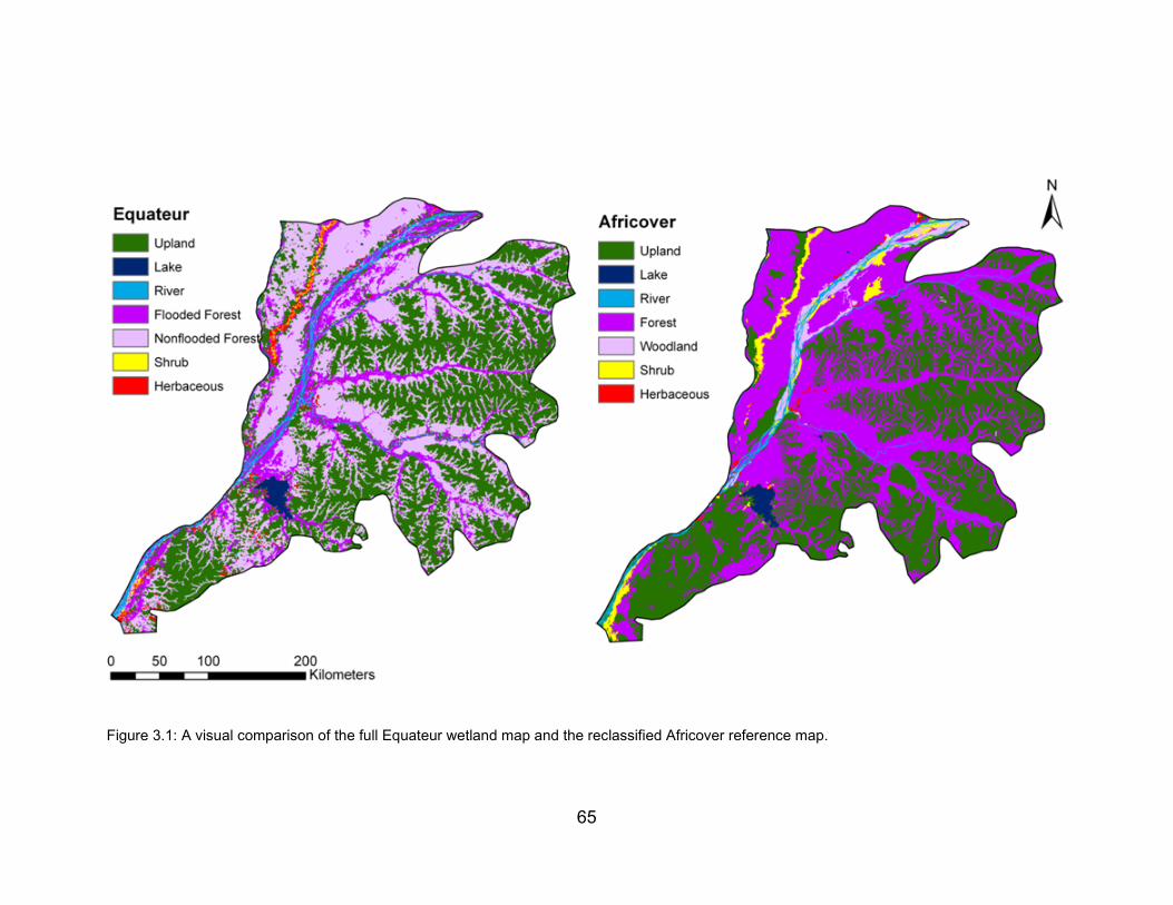
65
Figure 3.1: A visual comparison of the full Equateur wetland map and the reclassified Africover reference map.
66
3.1.1 Floodplain Forest and Woodland Misclassifications
Several sources indicate that almost the entire floodplain is covered by
closed forest canopy and is either permanently or intermittently flooded (Hughes
et al. 1992, De Grandi et al. 2000, Mayaux et al. 2002). This is in agreement with
Africover (Figure 3.1). According to the parallel-piped classifier adapted from
Hess et al. (2003), the majority of the floodplain environment is considered
floodplain woodland, or to have a tree canopy cover between 25% and 60% and
to be semi-permanently to permanently flooded. Because no ecological
distinction is made in descriptive (Hughes et al. 1992) or visual (De Grandi et al.
2000, Mayaux et al. 2002) accounts of the area that explain the pattern of
floodplain forest and woodland shown in the Equateur wetlands map, it is likely
that ecologically there is little or no difference between the vegetation type or
canopy closure of the forest and woodland classes.
While the vegetation classification is the same, the hydrological
classification is not. The hydrological definitions and indicators differ: for an
Equateur object to be classified as flooded, the area must show water above the
surface at the time of observation; for an Africover polygon to be classified as
flooded, its hydrology is inferred from vegetation that indicates the area has a
water table at or near the surface of the ground not necessarily at the time of
observation, but for at least two months of the year. Therefore, the hydrology
67
classifiers differ with respect to time: the Equateur classifier is based on two
instantaneous points in time, whereas the Africover classifier is not one of flood
extent but hydrophytic vegetation extent. This explanation is consistent with the
distribution of floodplain forest in the Equateur wetlands map, where the brightest
floodplain wetlands are next to rivers. This is expected when interpreting L-HH
radar response. Since floodplain woodland is likely the same or similar to
floodplain forest in vegetation structure and canopy closure, floodplain woodland
is a misnomer: in the Equateur wetlands map, it is likely also floodplain forest, but
nonflooded. Although the remaining misclassifications in other classes are
comparatively minor in relation to this error, the accuracies and their likely
explanations are provided below.
3.1.2 Upland
For the upland class, producer’s and user’s accuracies are approximately
equal at 74% and 78% respectively (Table 3.1). In both cases, the majority of the
error is the result of confusion with a single class. About 84% of the error
associated with producer’s accuracy (omission error) is confusion with
nonflooded floodplain forest (formerly floodplain woodland). Approximately 93%
of the error associated with user’s accuracy (commission error) is confusion with
Africover’s forest class. In terms of quantification, the Equateur upland class
68
approximates Africover’s upland class well with 4% fewer upland pixels (Table
3.2).
The source of greatest confusion is the difference between the
distributions of upland and floodplain areas (flooded and nonflooded floodplain
forest). While they generally approximate visually (Figure 3.1), there are
explanations for their small though consistent discrepancies.
The first is that the boundaries of the largest upland areas are scaled back
when compared to the Africover map (Figure 3.1). This is likely a result of the
different sensitivities of L-HH radar and optical imagery to forest canopies, as
well as a result of the subjective nature of delineating boundaries between
landcovers with a relatively fuzzy transition in optical imagery, as the transition
between forest types is extremely gradual in this region (Hughes et al. 1992). De
Grandi et al. (2000a) found this to be the most likely explanation for the
discrepancies between their C-VV radar-based swamp forest map and the optical
imagery based reference map of the region. This explains much of why the
quantity of upland is lower (by 4% or 233,350 pixels) and floodplain is higher (by
3% or 218,331 pixels) by nearly the equivalent amount in the Equateur wetlands
map (Table 3.2).
A second, though comparatively minor, explanation is that the Equateur
method does not allow floodplain to exist as an isolated area inside an upland
69
region. This is based on the reasoning that floodplain is an environment
continuous with running water bodies. It is for this reason that the upland rule
implies that no upland object may overlap with the HydroSHEDS River vector. In
the Africover map, however, there are several instances where secondary
floodplain appears to be cut off from the primary floodplain, which would also
cause the Equateur method to produce comparatively less upland and more
floodplain (Figure 3.1). These “cut offs” do not necessarily mean that there is no
hydrologic connectivity between the secondary and primary floodplains, but
rather that the floodplain was not discernible from the LANDSAT imagery (e.g., in
the case of a narrow gorge).
Finally, although the minimum mapping area is smaller for Africover (34 ha
vs. 50 ha), the Equateur map exhibits many small upland areas along all river
courses where Africover shows none (Figure 3.1). The heightened sensitivity to
upland of this method would slightly increase the quantity of upland compared to
the less-sensitive Africover method, which uses only optical data (and thus the
spectral reflectance of vegetation canopy) to derive landcover classes. As De
Grandi et al. (2000a) and Mayaux et al. (2000) note, the visual interpretation of
satellite imagery tends to eliminate small and narrow features, and this is likely
responsible for the difference.
70
3.1.3 Lake
Of all classifications, producer’s and user’s accuracies are highest for lake
at 96% and 97% respectively (Table 3.1). Most of the omission error is explained
by confusion with flooded forest (46%), herbaceous (22%) and nonflooded forest
(18%). Most of the commission error is explained by confusion with upland
(47%) and forest (33%). In terms of quantification, the Equateur lake class
closely matches the Africover lake class, underestimating it by 2% (Table 3.2).
The lake classification is both well quantified and located. This is not
surprising given the ease of identifying open water with both optical and radar
data and the accuracy of the SWBD ancillary dataset, whose overlap with open
water objects serves as the primary rule for this class. The extent of lake area is
slightly less in the Equateur wetlands map which may be a consequence of
greater flooding during the Africover imagery acquisition compared to the timing
of the SRTM data collection. Overall, the lake class is very well represented in
this method.
3.1.4 River
Producer’s and user’s accuracies are similar for the river class at 84% and
79% respectively (Table 3.1). The omission error is composed of confusion with
forest (71%) and nonflooded forest (13%). Commission errors are split among all
of the vegetated classes: forest (32%), upland (23%), woodland (20%), shrub
71
(14%), and herbaceous (11%). Compared to Africover, the quantity of the
Equateur river class approximates well, overestimating by 5% (Table 3.2).
This over-quantification may be the result of the greater sensitivity of radar
to rivers than optical sensors, particularly as L-HH radar is capable of penetrating
vegetation canopies that may otherwise hide shorelines in optical imagery. This
could also be explained by the tendency of eliminating small (or in this case,
narrow) features during the visual interpretation of Africover. River
overestimation may also be the consequence of differences in objectivity and
consistency between the methods of map making. The multi-resolution and
spectral segmentation procedures identify small, spectrally distinct objects
objectively. The Busira River, for example, terminates earlier in the Africover
dataset compared to the Equateur map. Compare this to the relatively early
termination of the Lopori and Maringa Rivers (Figure 3.1). This can explain the
commission errors of river with the flooded vegetation classes. Generally, the
river class is well classified without significant quantification or location error.
3.1.5 Floodplain Shrub
Of all classifications, producer’s accuracy is lowest for shrub at 13%, with
a user’s accuracy of 85% (Table 3.1). Most of the omission error is confusion
with flooded forest (35%), herbaceous (30%), and nonflooded forest (26%). Most
of the commission error is confusion with upland (49%), forest (30%), and
72
herbaceous (15%). In terms of quantification, 84% less shrub is quantified by the
Equateur method compared to Africover (Table 3.2).
The clearest example of shrub underestimation occurs on the left bank of
the Congo River as it enters the area in the north and along the left shoreline
further south (Figure 3.1). There is also considerable confusion with herbaceous
vegetation for shrub along the Giri River and on the left bank of the Congo River
where it exits the Equateur district (Figure 3.1). The Giri River is well known to
show complex mosaics of flooded herbaceous and shrub vegetation (Hughes et
al. 1992, Mayaux et al. 2002). It also is the most accurate in terms of the low-
and high-water mosaics representing true low- and high-water conditions
(Rosenqvist and Birkett 2002). Therefore, the unidirectional change in stage
assumed during the development of the Hess et al. (2003) parallel-piped
classifier holds truest for this river and, when corroborated with the Directory of
African Wetlands and a previous wetland map of the region (Mayaux et al. 2002),
is likely more representative of ground truth than Africover. The other areas of
shrub vegetation cannot be verified. Visually, the shrub class of Africover tends
to coincide with the shrub and herbaceous classes of the Equateur map, except
for the large patch near Bolombo (Figure 3.1).
73
3.1.6 Floodplain Herbaceous Vegetation
Producer’s accuracy is 20% and user’s accuracy is 6% for the herbaceous
class (Table 3.1). The error associated with the low producer’s accuracy comes
from confusion with flooded forest (38%), nonflooded forest (30%), and river
(21%). The commission error is explained mostly by confusion with shrub (49%)
and upland (37%). The Equateur method over-quantifies herbaceous cover by
259% or approximately 112,000 pixels; the largest quantification discrepancy
(Table 3.2).
The majority of the shrub confusion occurs along the Giri River, which is
known to contain mostly herbaceous vegetation, both rooted and floating
(Hughes et al. 1992, De Grandi et al. 2000a). Large sedges also occur along the
Giri, and it is well documented that emergent herbaceous vegetation greater than
1.5 m in height can be mistaken for shrub in L-band frequencies (Silva et al.
2008), and that interpretation of such vegetation from LANDSAT imagery is often
confused for shrub as well. It is possible that this can also explain the confusion
between flooded herbaceous and shrub on the southern left bank of the Congo
River, but no documentation exists to confirm this. It is important to note that
where Africover indicates flooded herbaceous (e.g., north of the confluence of the
Ruki River with the Congo River and along the right bank of the Congo in the
northern reach), the Equateur method also shows flooded herbaceous vegetation
74
(Figure 3.1). Therefore, it is reasonable to assume that the method presented
here better represents flooded herbaceous vegetation than Africover, especially
along the Giri River.
3.2 Simplified Wetlands Map
The simplified wetlands map includes five classes: upland, lake, river, tall
vegetation and short vegetation. The tall vegetation class is the combination of
the flooded floodplain forest and nonflooded floodplain forest classes. The short
vegetation class is the combination of the floodplain shrub and herbaceous
vegetation classes. The simplified wetlands map and corresponding Africover
map are shown in Figure 3.2.
Strategically collapsing the classes from seven to five increased the
overall accuracy from 47% to 76% and doubled the KIA from 28% to 57% (Table
3.3). All of the classes were well quantified except short vegetation, which was
underestimated by 38% (Table 3.4).
3.2.1 Tall Floodplain Vegetation
The tall vegetation class combines both the floodplain forest and woodland
classes to effectively become a flooded trees class. The producer’s and user’s
accuracies are 80% and 76% respectively (Table 3.3). Nearly all of the omission
and commission error is with upland at 96% and 86% respectively. Compared to
75
Africover, the tall vegetation class is well quantified with 6% difference (Table
3.4).
3.2.2 Short Floodplain Vegetation
The short vegetation class collapses the shrub and herbaceous classes of
the full wetland map into a single class. The producer’s and user’s accuracies
are 37% and 60% respectively (Table 3.3). Most of the producer’s error is
explained by confusion with tall vegetation (84%), and user’s error is associated
with confusion with upland (72%) and tall vegetation (22%). Quantification of
short vegetation by the Equateur method is 38% less than indicated by the
corresponding Africover class (Table. 3.4).
The shrub and herbaceous classes which make up the short vegetation
class remain difficult to correspond with Africover. L-HH is well known to be most
sensitive to flooded forest with decreasing sensitivity to shrub and herbaceous
vegetation (Hess et al. 2003). This may explain the confusion between the two
classes, but not its confusion with the tall vegetation class.
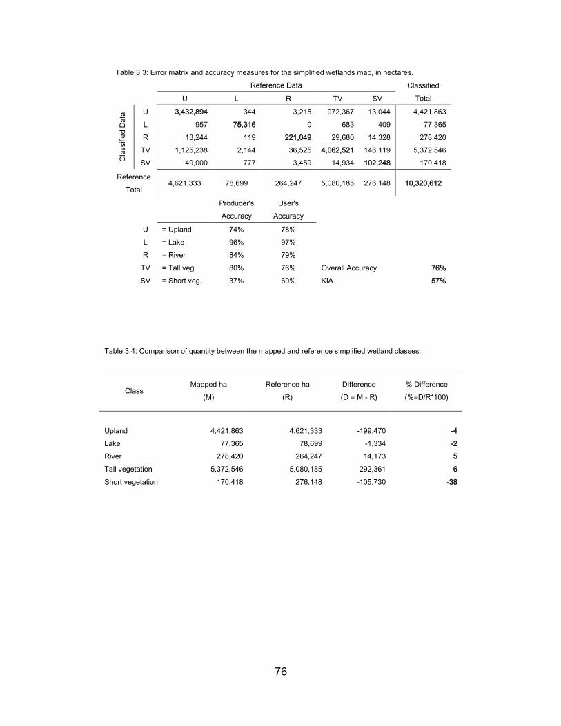
76
Table 3.3: Error matrix and accuracy measures for the simplified wetlands map, in hectares.
Reference Data Classified
Total U L R TV SV
Cla
ssifie
d D
ata
U 3,432,894 344 3,215 972,367 13,044 4,421,863
L 957 75,316 0 683 409 77,365
R 13,244 119 221,049 29,680 14,328 278,420
TV 1,125,238 2,144 36,525 4,062,521 146,119 5,372,546
SV 49,000 777 3,459 14,934 102,248 170,418
Reference
Total 4,621,333 78,699 264,247 5,080,185 276,148 10,320,612
Producer's
Accuracy
User's
Accuracy
U = Upland 74% 78%
L = Lake 96% 97%
R = River 84% 79%
TV = Tall veg. 80% 76% Overall Accuracy 76%
SV = Short veg. 37% 60% KIA 57%
Table 3.4: Comparison of quantity between the mapped and reference simplified wetland classes.
Class Mapped ha
(M)
Reference ha
(R)
Difference
(D = M - R)
% Difference
(%=D/R*100)
Upland 4,421,863 4,621,333 -199,470 -4
Lake 77,365 78,699 -1,334 -2
River 278,420 264,247 14,173 5
Tall vegetation 5,372,546 5,080,185 292,361 6
Short vegetation 170,418 276,148 -105,730 -38
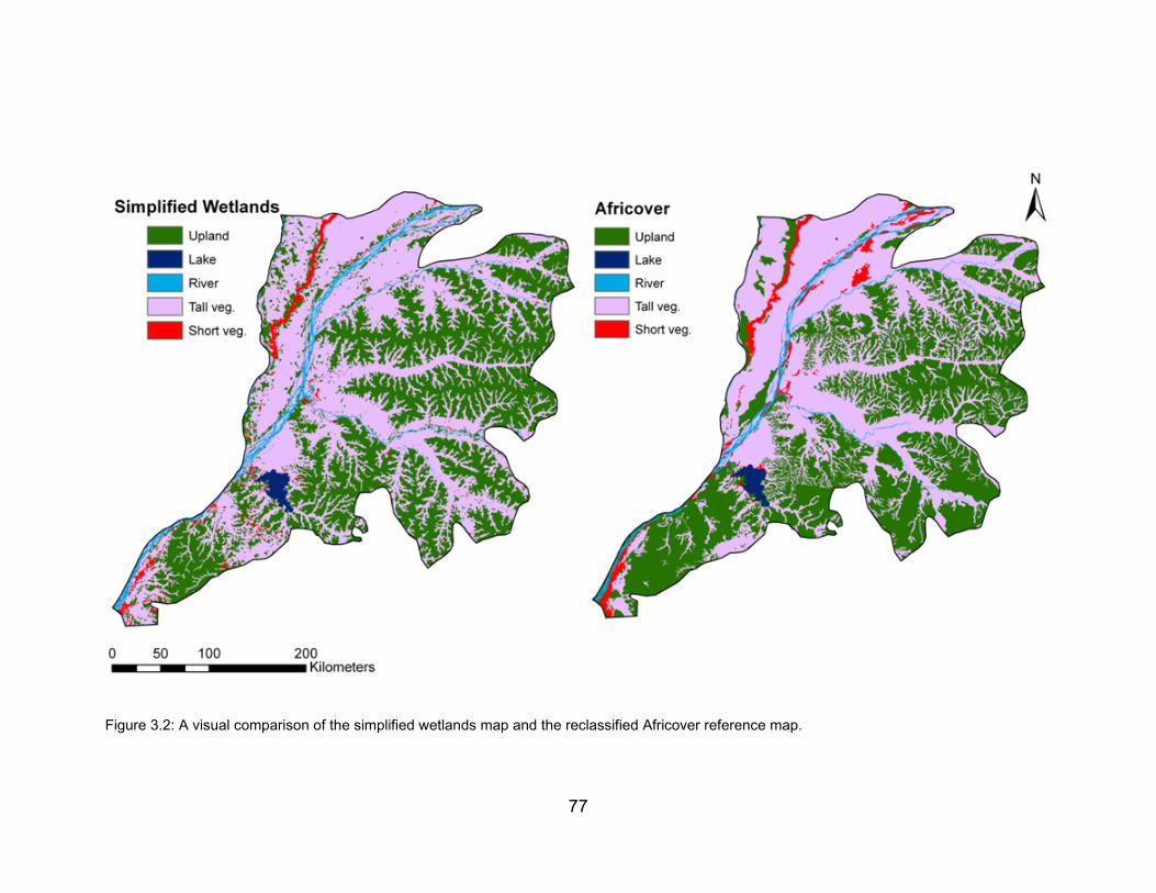
77
Figure 3.2: A visual comparison of the simplified wetlands map and the reclassified Africover reference map.
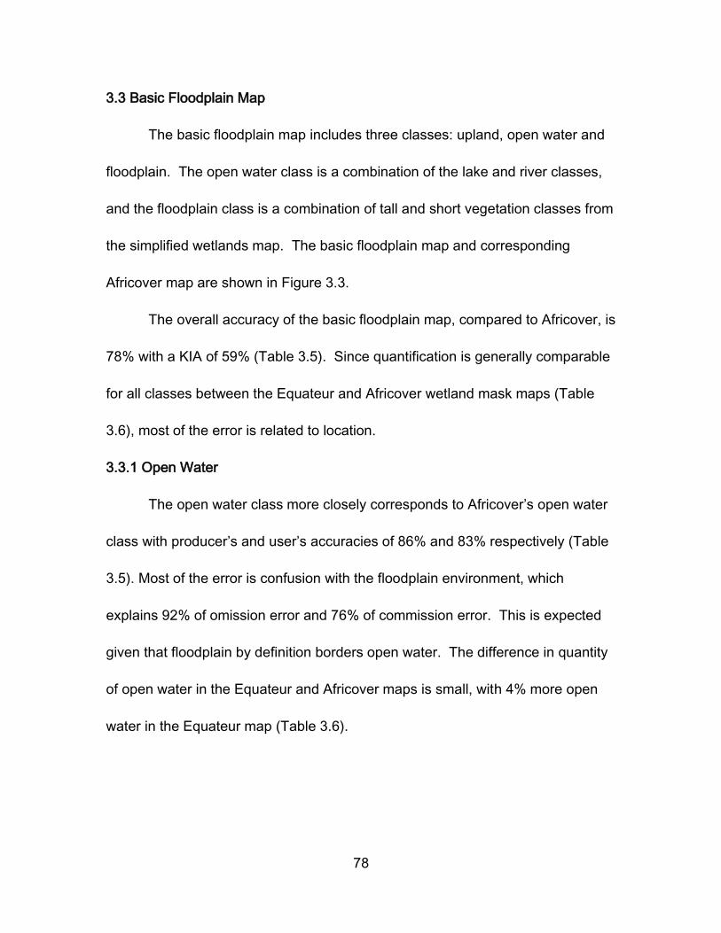
78
3.3 Basic Floodplain Map
The basic floodplain map includes three classes: upland, open water and
floodplain. The open water class is a combination of the lake and river classes,
and the floodplain class is a combination of tall and short vegetation classes from
the simplified wetlands map. The basic floodplain map and corresponding
Africover map are shown in Figure 3.3.
The overall accuracy of the basic floodplain map, compared to Africover, is
78% with a KIA of 59% (Table 3.5). Since quantification is generally comparable
for all classes between the Equateur and Africover wetland mask maps (Table
3.6), most of the error is related to location.
3.3.1 Open Water
The open water class more closely corresponds to Africover’s open water
class with producer’s and user’s accuracies of 86% and 83% respectively (Table
3.5). Most of the error is confusion with the floodplain environment, which
explains 92% of omission error and 76% of commission error. This is expected
given that floodplain by definition borders open water. The difference in quantity
of open water in the Equateur and Africover maps is small, with 4% more open
water in the Equateur map (Table 3.6).
79
Table 3.5: Error matrix and accuracy measures for the basic floodplain map, in hectares.
Reference Data Classified Total
U OW FP
Cla
ssifie
d
Data
U 3,432,894 3,559 985,411 4,421,863
OW 14,201 296,483 45,101 355,785
FP 1,174,238 42,905 4,325,822 5,542,965
Reference
Total 4,621,333 342,946 5,356,333 10,320,612
Producer's
Accuracy
User's
Accuracy
U = Upland 74% 78%
OW = Open water 86% 83% Overall Accuracy 78%
FP = Floodplain 81% 78% KIA 59%
Table 3.6 Comparison of quantity between the mapped and reference basic floodplain classes.
Class Mapped ha
(M)
Reference ha
(R)
Difference
(D = M - R)
% Difference
(%=D/R*100)
Upland 4,421,863 4,621,333 -199,470 -4
Open water 355,785 342,946 12,838 4
Floodplain 5,542,965 5,356,333 186,631 3
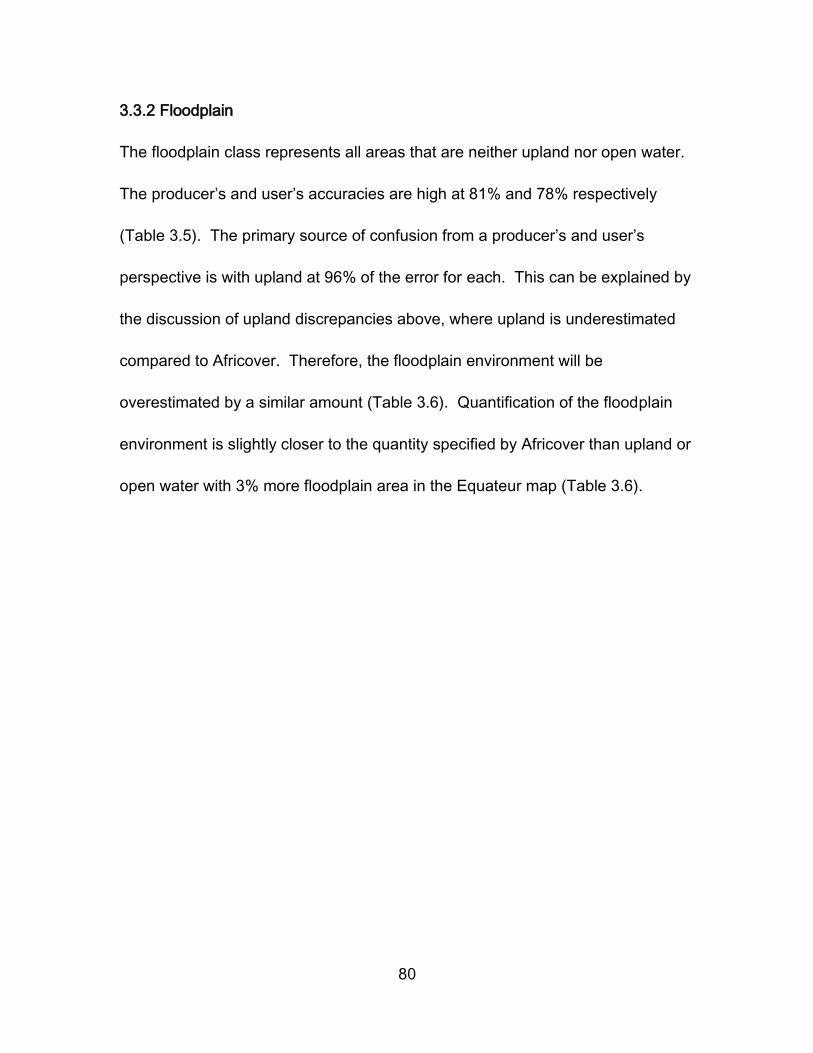
80
3.3.2 Floodplain
The floodplain class represents all areas that are neither upland nor open water.
The producer’s and user’s accuracies are high at 81% and 78% respectively
(Table 3.5). The primary source of confusion from a producer’s and user’s
perspective is with upland at 96% of the error for each. This can be explained by
the discussion of upland discrepancies above, where upland is underestimated
compared to Africover. Therefore, the floodplain environment will be
overestimated by a similar amount (Table 3.6). Quantification of the floodplain
environment is slightly closer to the quantity specified by Africover than upland or
open water with 3% more floodplain area in the Equateur map (Table 3.6).
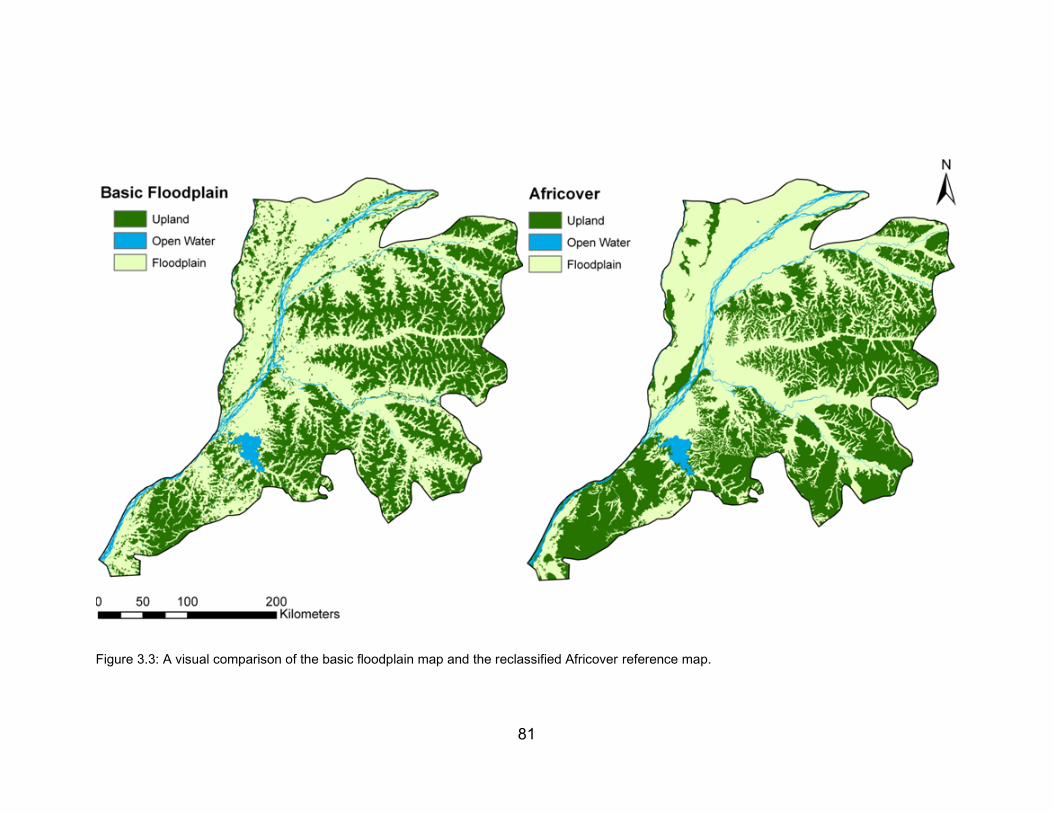
81
Figure 3.3: A visual comparison of the basic floodplain map and the reclassified Africover reference map.
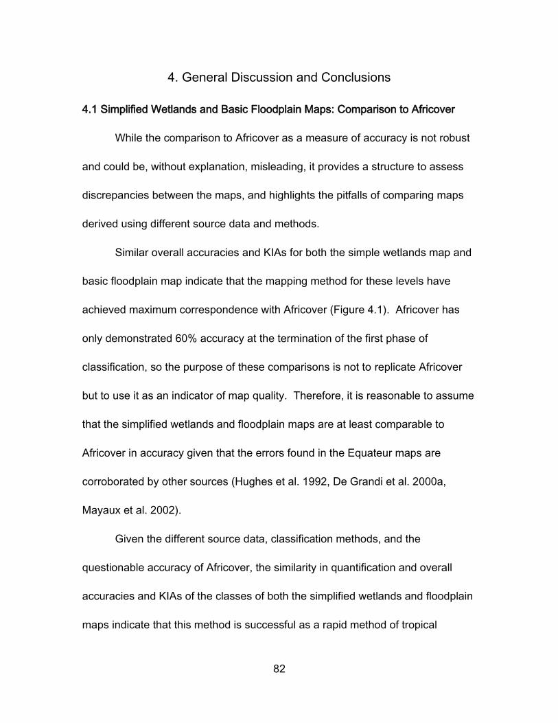
82
4. General Discussion and Conclusions
4.1 Simplified Wetlands and Basic Floodplain Maps: Comparison to Africover
While the comparison to Africover as a measure of accuracy is not robust
and could be, without explanation, misleading, it provides a structure to assess
discrepancies between the maps, and highlights the pitfalls of comparing maps
derived using different source data and methods.
Similar overall accuracies and KIAs for both the simple wetlands map and
basic floodplain map indicate that the mapping method for these levels have
achieved maximum correspondence with Africover (Figure 4.1). Africover has
only demonstrated 60% accuracy at the termination of the first phase of
classification, so the purpose of these comparisons is not to replicate Africover
but to use it as an indicator of map quality. Therefore, it is reasonable to assume
that the simplified wetlands and floodplain maps are at least comparable to
Africover in accuracy given that the errors found in the Equateur maps are
corroborated by other sources (Hughes et al. 1992, De Grandi et al. 2000a,
Mayaux et al. 2002).
Given the different source data, classification methods, and the
questionable accuracy of Africover, the similarity in quantification and overall
accuracies and KIAs of the classes of both the simplified wetlands and floodplain
maps indicate that this method is successful as a rapid method of tropical
83
floodplain wetland classification at these levels of classification. This is possible
because the L-HH radar and topography datasets are more sensitive to and
consistent with the physiognomic-hydrologic wetland classification scheme used,
and because the object-oriented segmentation and classification is a more
objective, semi-automated, and consistent approach to image analysis than
visual interpretation.
Figure 4.1: Accuracy obtained using Africover as reference data for the three levels of wetland
class aggregation.
4.2 Simplified Wetlands and Basic Floodplain Maps: Comparison to other maps
Further, though qualitative, insight to the quality of these maps is gained
from the visual comparisons of the simple wetlands and floodplain maps to
leading, similar maps of the region.
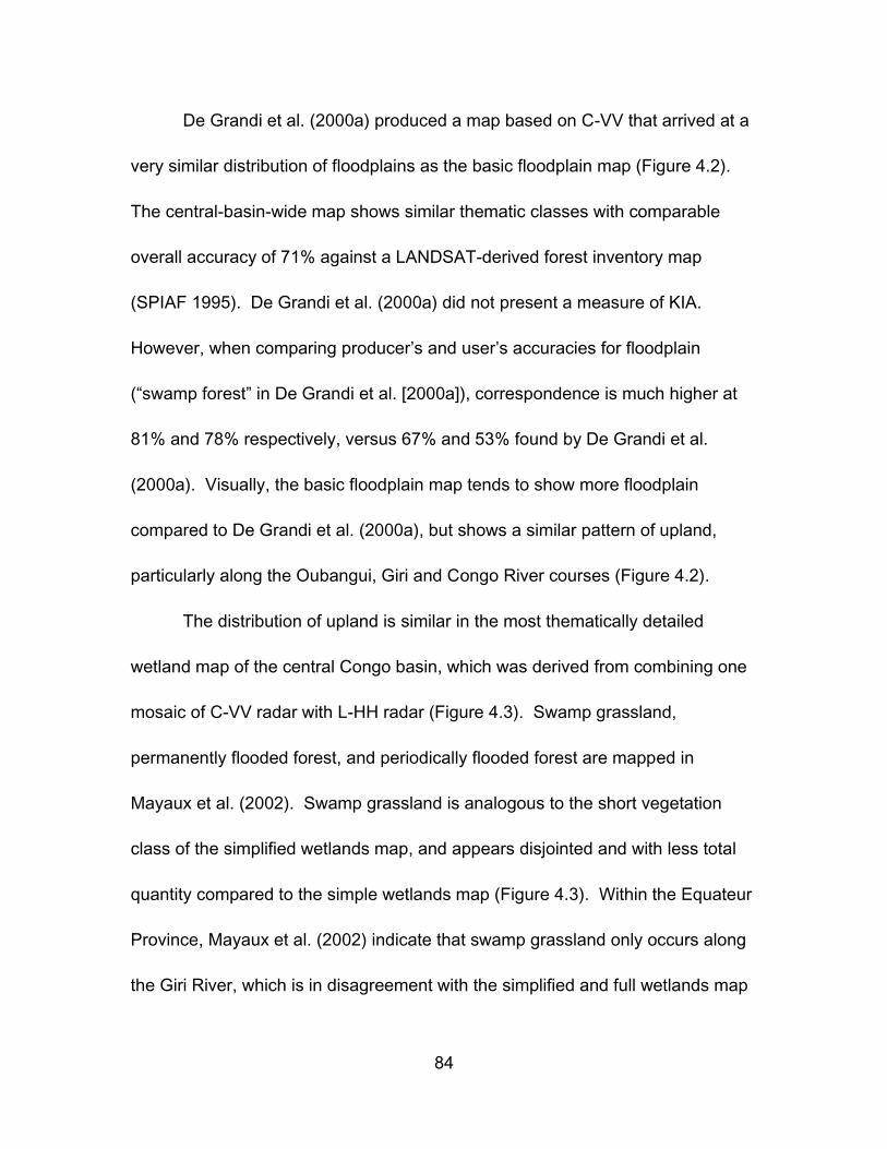
84
De Grandi et al. (2000a) produced a map based on C-VV that arrived at a
very similar distribution of floodplains as the basic floodplain map (Figure 4.2).
The central-basin-wide map shows similar thematic classes with comparable
overall accuracy of 71% against a LANDSAT-derived forest inventory map
(SPIAF 1995). De Grandi et al. (2000a) did not present a measure of KIA.
However, when comparing producer’s and user’s accuracies for floodplain
(“swamp forest” in De Grandi et al. [2000a]), correspondence is much higher at
81% and 78% respectively, versus 67% and 53% found by De Grandi et al.
(2000a). Visually, the basic floodplain map tends to show more floodplain
compared to De Grandi et al. (2000a), but shows a similar pattern of upland,
particularly along the Oubangui, Giri and Congo River courses (Figure 4.2).
The distribution of upland is similar in the most thematically detailed
wetland map of the central Congo basin, which was derived from combining one
mosaic of C-VV radar with L-HH radar (Figure 4.3). Swamp grassland,
permanently flooded forest, and periodically flooded forest are mapped in
Mayaux et al. (2002). Swamp grassland is analogous to the short vegetation
class of the simplified wetlands map, and appears disjointed and with less total
quantity compared to the simple wetlands map (Figure 4.3). Within the Equateur
Province, Mayaux et al. (2002) indicate that swamp grassland only occurs along
the Giri River, which is in disagreement with the simplified and full wetlands map
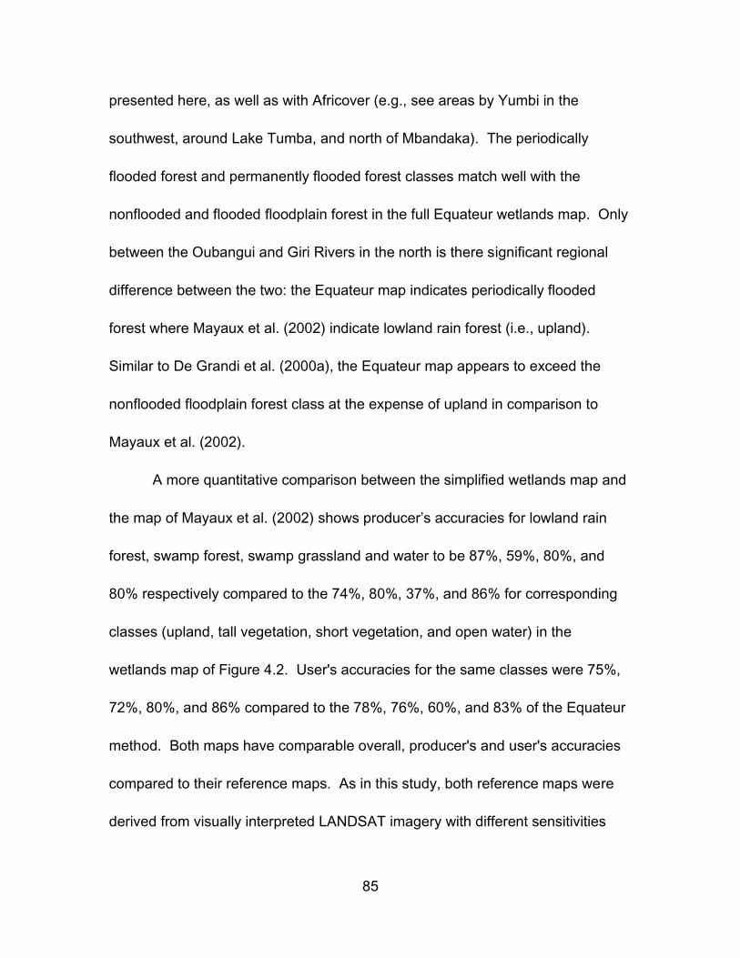
85
presented here, as well as with Africover (e.g., see areas by Yumbi in the
southwest, around Lake Tumba, and north of Mbandaka). The periodically
flooded forest and permanently flooded forest classes match well with the
nonflooded and flooded floodplain forest in the full Equateur wetlands map. Only
between the Oubangui and Giri Rivers in the north is there significant regional
difference between the two: the Equateur map indicates periodically flooded
forest where Mayaux et al. (2002) indicate lowland rain forest (i.e., upland).
Similar to De Grandi et al. (2000a), the Equateur map appears to exceed the
nonflooded floodplain forest class at the expense of upland in comparison to
Mayaux et al. (2002).
A more quantitative comparison between the simplified wetlands map and
the map of Mayaux et al. (2002) shows producer’s accuracies for lowland rain
forest, swamp forest, swamp grassland and water to be 87%, 59%, 80%, and
80% respectively compared to the 74%, 80%, 37%, and 86% for corresponding
classes (upland, tall vegetation, short vegetation, and open water) in the
wetlands map of Figure 4.2. User's accuracies for the same classes were 75%,
72%, 80%, and 86% compared to the 78%, 76%, 60%, and 83% of the Equateur
method. Both maps have comparable overall, producer's and user's accuracies
compared to their reference maps. As in this study, both reference maps were
derived from visually interpreted LANDSAT imagery with different sensitivities
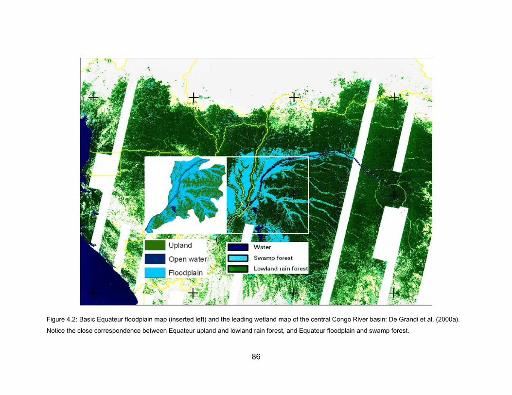
86
Figure 4.2: Basic Equateur floodplain map (inserted left) and the leading wetland map of the central Congo River basin: De Grandi et al. (2000a).
Notice the close correspondence between Equateur upland and lowland rain forest, and Equateur floodplain and swamp forest.
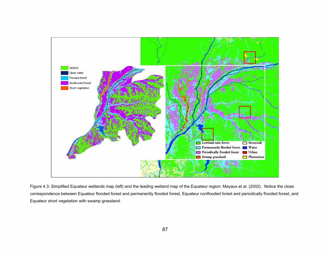
87
Figure 4.3: Simplified Equateur wetlands map (left) and the leading wetland map of the Equateur region: Mayaux et al. (2002). Notice the close
correspondence between Equateur flooded forest and permanently flooded forest, Equateur nonflooded forest and periodically flooded forest, and
Equateur short vegetation with swamp grassland.
88
that suggest that discrepancies are actually improvements over their respective
reference maps (Mayaux et al. 2002). With the exception of overestimating the
area of floodplain, the Equateur method appears to approximate the classes of
the leading wetland maps of the region well, and may produce a more accurate
short vegetation class.
4.3 Full Equateur Wetlands Map
The Equateur method is also useful for providing additional classes
previously unmapped in the region, distinguishing between shrub and
herbaceous vegetation. However, the accuracy of these classes can only
currently be verified by the single available high-resolution landcover map of the
region: Africover. As indicated in the results presented above, the distribution of
shrub and herbaceous vegetation between the Equateur and Africover maps is
similar. The Equateur map shows considerably more herbaceous vegetation
where Africover indicates shrub, particularly along the Giri River, but other
descriptive and mapping sources support the results of the Equateur map. This,
in addition to the visual comparison of the flooded floodplain forest, nonflooded
floodplain forest, and short vegetation classes to Mayaux et al. (2002) above,
indicates that the accuracy of the full Equateur wetlands map is higher than
indicated by its comparison to Africover, but it is unknown to what degree.
89
An interesting failure of the classification scheme was to correctly identify
floodplain woodland. This class was adapted directly from the parallel-piped
classifier derived in Hess et al. (2003) from the PDF of flooded woodland found
from training samples in the central Amazon. When comparing the distributions
of classes to the map of Mayaux et al. (2002), it is evident that the flooded
woodland classifier of Hess et al. (2003) represents nonflooded forest in the full
Equateur wetlands map. Since L-HH is sensitive to volumetric scattering in the
canopy (increasing backscatter with denser canopy) and to flooded, vegetated
surfaces via a double-bounce mechanism, it is possible that the dual-mosaic
response of the flooded woodland in the central Amazon (high double bounce
return, lower volumetric scattering) approximates that of nonflooded forest in the
central Congo (low double bounce return, higher volumetric scattering). This is
supported by a comparison of the PDFs illustrated in Hess et al. (2003), which
shows the flooded woodland class PDF entirely overlapping and peaking
similarly to the narrower nonflooded forest class PDF (Figure 4.4).
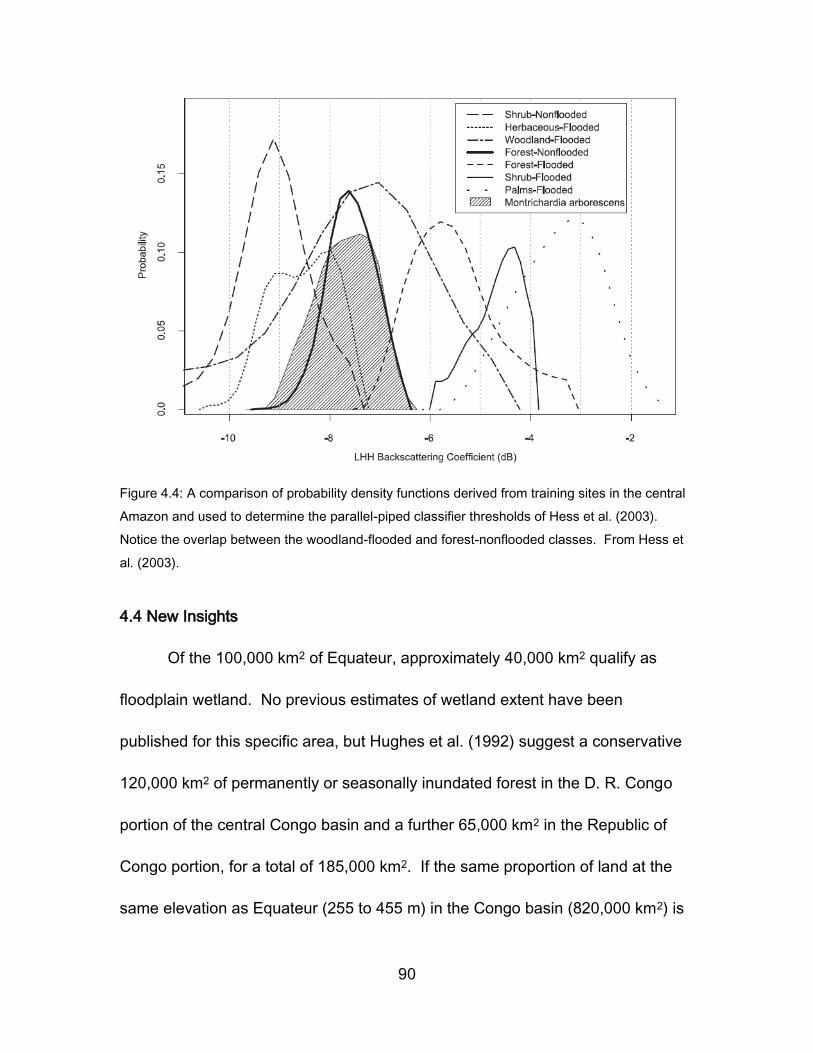
90
Figure 4.4: A comparison of probability density functions derived from training sites in the central
Amazon and used to determine the parallel-piped classifier thresholds of Hess et al. (2003).
Notice the overlap between the woodland-flooded and forest-nonflooded classes. From Hess et
al. (2003).
4.4 New Insights
Of the 100,000 km2 of Equateur, approximately 40,000 km2 qualify as
floodplain wetland. No previous estimates of wetland extent have been
published for this specific area, but Hughes et al. (1992) suggest a conservative
120,000 km2 of permanently or seasonally inundated forest in the D. R. Congo
portion of the central Congo basin and a further 65,000 km2 in the Republic of
Congo portion, for a total of 185,000 km2. If the same proportion of land at the
same elevation as Equateur (255 to 455 m) in the Congo basin (820,000 km2) is
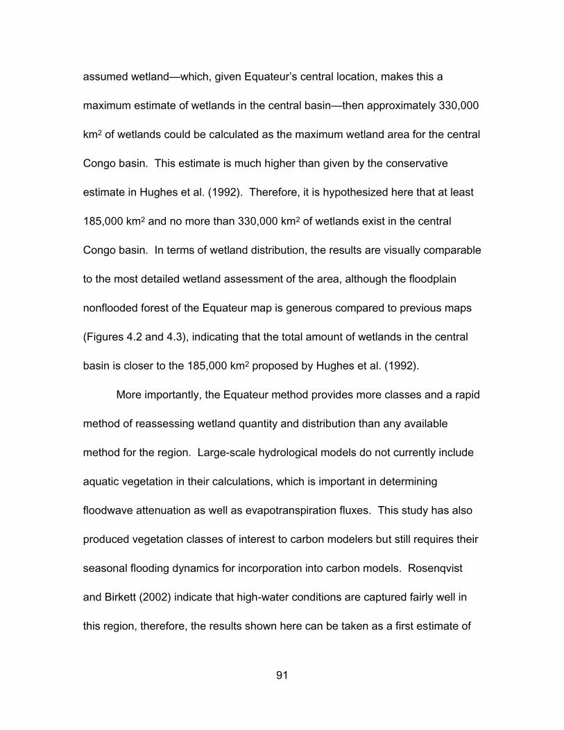
91
assumed wetland—which, given Equateur’s central location, makes this a
maximum estimate of wetlands in the central basin—then approximately 330,000
km2 of wetlands could be calculated as the maximum wetland area for the central
Congo basin. This estimate is much higher than given by the conservative
estimate in Hughes et al. (1992). Therefore, it is hypothesized here that at least
185,000 km2 and no more than 330,000 km2 of wetlands exist in the central
Congo basin. In terms of wetland distribution, the results are visually comparable
to the most detailed wetland assessment of the area, although the floodplain
nonflooded forest of the Equateur map is generous compared to previous maps
(Figures 4.2 and 4.3), indicating that the total amount of wetlands in the central
basin is closer to the 185,000 km2 proposed by Hughes et al. (1992).
More importantly, the Equateur method provides more classes and a rapid
method of reassessing wetland quantity and distribution than any available
method for the region. Large-scale hydrological models do not currently include
aquatic vegetation in their calculations, which is important in determining
floodwave attenuation as well as evapotranspiration fluxes. This study has also
produced vegetation classes of interest to carbon modelers but still requires their
seasonal flooding dynamics for incorporation into carbon models. Rosenqvist
and Birkett (2002) indicate that high-water conditions are captured fairly well in
this region, therefore, the results shown here can be taken as a first estimate of
92
maximum wetland extent for Equateur. Although flooding dynamics are not
captured in this study, it is not a limitation of the method but rather of the
datasets. Upon further releases of L-band datasets for the region, this method
could be expanded to include the full physiognomic-hydrologic classifications
used in Hess et al. (2003). The seasonal wetland distribution information that
would result can be used in conjunction with field measurements of methane
emissions, as calculated for the Amazon by Melack et al. (2004). The same
information on the type and distribution of wetlands illustrated in this study can be
used for fishery management, as fishing is a major source of protein and
economic activity in the region. However, one wetland class that these data
could not resolve that is important to ecological and cultural welfare is Raphia
palms. It is well documented that Raphia spp. (a cosmopolitan wetland palm) is
the primary habitat of the otherwise little studied and endemic lowland gorilla, in
addition to significant food and cultural value (grubs, wine) to the local Bantu and
Pygmy peoples (Hart and Hart 1986). Africover includes a custom Raphia spp.
class in the D. R. Congo dataset, and these polygon outlines were used for
training to identify other floodplain objects that qualified as Raphia spp. The
radar backscatter was not distinguishable from nonflooded floodplain forest, and
was left out of the classification. In this case, optical imagery would be of use in
capturing this special class, as was successfully done by Hamilton et al. (2007)
93
using LANDSAT imagery in conjunction with radar and elevation data over the
Madre de Dios subbasin of the Amazon River basin. It is also possible that the
multi-polarized radar imagery now made available by the ALOS/PALSAR satellite
could also distinguish this class, however, no study has yet determined this.
4.5 Limitations and Future Work
A clear limitation of this method is the availability of dual-season L-HH
datasets. The radar datasets used here exist—though only in dual-season form
for the Amazon and the Congo—for the rest of the tropics. Dual-season L-HH
mosaics were essential for distinguishing the flooded shrub and herbaceous
vegetation classes. With single-season L-HH data, only flooded and nonflooded
forest wetland classes could be reliably classified. The multipolarized
ALOS/PALSAR L-band sensor has since succeeded the JERS-1/SAR L-HH
sensor, and currently releases 500 m mosaics of the African continent every
cycle, or 46 days. In addition, a new radar dataset based on ALOS/PALSAR
consisting of 50 m resolution, orthorectified mosaics is soon to be released from
the EC JRC with the objective of capturing low- and high-water conditions over
the Congo basin.
However, even with well-timed L-band radar mosaics, Hess et al. (2003)
found that their classifier did not perform well in tidally inundated areas,
interfluvial white-sand wetlands with low biomass shrubs and sedges, and in
94
wetlands within large savannas where there is low-biomass and the herbaceous
vegetation is rooted and emergent rather than high-biomass and floating. The
Congo River has little tidally inundated area at its mouth but does exhibit
extensive savannas to the north and south of the central basin. Important, large
wetland systems lie in the southern portion of the basin such as in the
Kamolondo Depression, where the Upemba Lakes and approximately 800,000
ha of forested and herbaceous wetlands occur (Hughes et al. 1992). Therefore,
the data and classifier presented here—though simpler than that used in Hess et
al. (2003)—may require changes to adapt to the vegetation and geomorphology
of different regions and (or) to capture important classes not included in this
wetland scheme.
Perhaps the most beneficial additional information would be an optical
dataset, which could further distinguish forest types and include species-specific
classifications such as Raphia spp. palms, which were indistinguishable from
flooded forest in Hess et al. (2003) and from nonflooded floodplain forest in this
study. Hamilton et al. (2007), for example, were successful identifying a Raphia
spp. palm class in a sub-basin classification of the Amazon using
LANDSAT/ETM+ imagery. Although the problem of cloud cover precludes
optical imagery from being the principle source of rapid tropical floodplain
wetland mapping method, the recent availability of optical, 300 m resolution
95
global composites from the MERIS/Globcover initiative could serve as a
complimentary dataset in future, large-scale wetland mapping studies, especially
as the multipolarized C-band ENVISAT/ASAR sensor is also employed in this
initiative to delineate wetland from humid tropical forests.
C-band radar data would also provide complimentary information by
improving the distinction between the herbaceous and shrub classes, since these
vegetation covers are difficult to distinguish between in the L-band wavelength.
Simard et al. (2002), for example, found that merging L-HH and C-VV data could
effectively map woody and herbaceous wetlands along the coast of Gabon. The
recent release of 150 m resolution C-band mosaics from the ENVISAT/ASAR
program could be incorporated to improve the accuracy of the short vegetation
classes of this method and to potentially make further differentiations between
forest types based on canopy backscatter signatures or texture.
The TERRA/ASTER 30 m global DEM was recently released for public
use, and exceeds the HydroSHEDS DEM in spatial resolution with approximately
the same accuracy (ASTER 2009). With a higher resolution DEM, sinuous
meader scrolls and smaller channel bars common to the floodplain environment
of large rivers could be detected. These objects could then be distinguished from
upland based on proximity to river and length-to-width ratios, for example.
96
4.6 Conclusions
This study has achieved a rapid method of tropical floodplain classification
comparable in thematic detail to the leading wetland map of the central Congo
basin (Mayaux et al. 2002) and in accuracy to the only publicly available, high
resolution wetland map of the region: Africover. It also provides a limit of
maximum wetland area in the central Congo basin and a first estimate of
floodplain shrub and herbaceous vegetation classes in the Equateur
administrative region. The method demonstrates the power of integrating several
wetland-relevant, digital datasets, and indicates that the parallel-piped classifier
derived from Hess et al. (2003) is valid for use in the central Congo basin with
the exception of confusing nonflooded floodplain forest for flooded woodland.
The addition of elevation and slope datasets and the HydroSHEDS Rivers vector
layer reduced the reliance on L-HH radar for the upland class, since it was found
that backscatter of upland overlapped with forest and herbaceous cover in the
parallel-piped classifier of Hess et al. (2003). The addition of the SWBD Lakes
dataset enabled the distinction of lakes from rivers. In addition, the study
provides further evidence that image segmentation is both a practical and
effective method for large raster dataset analysis (Costa et al. 2002, Hess et al.
2003, Durieux et al. 2007).
97
There are several advantages to the object-oriented approach employed
in this study: the ability to incorporate other datasets in a transparent way (via the
process tree) without complex image fusion procedures involved with traditional
pixel classifications. This capability allows the method to be customized or
improved upon with the growing number of global and near-global digital
datasets relevant to wetland mapping. The object-oriented approach is also
unbiased compared to visual interpretation and manual delineation of satellite
imagery (e.g., Africover).
There are limitations, however, since classification rules will likely need to
be adapted to different geomorphological and ecological settings outside of the
central basin. Also, the scale parameters reported here do not refer to any
known algorithm, only to the scale factor unique to the image analysis software
used in this study. Therefore, it is unknown how the data are actually treated to
create image objects of the appropriate size and shape. Lastly, dual-season
radar data are necessary to determine shrub and herbaceous vegetation from L-
HH radar. However, adding C-band radar or potentially multi-polarized L-band
data may provide enough information to better distinguish these classes.
Greater availability of high-resolution, large scale optical composites may also
improve classification accuracy and would also provide more ecologically
important wetland classes such as Raphia spp. palm stands.
98
As no extensive fieldwork has been conducted to verify Africover, the
accuracy of this method cannot be ascertained, though it is comparable to
previous maps of the region. While computer classification of remote sensing
data should never supersede field observations and data, their outputs can be
used to improve hydrological and biogeochemical models, in addition to affecting
science-based conservation strategies that are urgently needed in many rapidly
developing tropical countries such as the D. R. Congo that depend upon many
floodplain wetland ecosystem services (Thieme et al. 2007).
A rapid method of tropical floodplain wetland mapping over a large area of
the central Congo floodplain has been produced with relevance to hydrologists,
biogeochemists, and conservationists that is comparable to the thematic detail
and accuracy of previous work in addition to providing two new classes of wide
interest: floodplain shrub and herbaceous vegetation. Africover is the only
dataset with comparable spatial and thematic detail; however, it suffers from a
dependency on cloud-free imagery that makes it difficult to acquire multi-
temporal imagery from different seasons, in addition to an inability to penetrate
dense tropical canopies to determine flood extent. Thematic detail is improved
with the Equateur method in comparison with Africover with better discrimination
between the shrub and herbaceous classes. The semi-automated nature of the
Equateur method also makes for a consistent and rapid method of monitoring
99
wetland classes in comparison to the interpretation of LANDSAT imagery used in
Africover. Finally, this study highlights the potential of wide area, high-resolution
L-HH radar and topography datasets for mapping tropical floodplain wetlands at
an appropriate scale for regional inventory and monitoring purposes, and can be
further improved by the growing availability of relevant, digital datasets and their
consistent, semi-automatic integration in an object-oriented analysis.
100
References
ASTER (2009). Features of ASTER DEM. Online at
http://www.ersdac.or.jp/GDEM/E/2.html
Ausseil, A., Dymond, J., & Shepherd, J. (2007). Rapid mapping and prioritisation
of wetland sites in the Manawatu–Wanganui region, New Zealand.
Environmental Management, 39, 316-325
Baker, C., Lawrence, R., Montague, C., & Patten, D. (2006). Mapping wetlands
and riparian areas using Landsat ETM+ imagery and decision-tree-based
models. Wetlands, 26, 465-474
Blake, S., Rogers, E., Fay, J., Ngangoue, M., & Ebeke, G. (1995). Swamp
gorillas in northern Congo. African Journal of Ecology, 33, 285-290
Bolstad, P. V. & Lillesand, T. M. (1992). Rule-based classification models –
flexible integration of satellite imagery and thematic spatial data.
Photogrammetric Engineering and Remote Sensing, 58, 965-971
Bultot, F. (1971). Atlas climatique du basin congolaise, vol. 3, température et
humidité de l’air, rosée, température du sol. Bruxelles, Belgium: Institut
National pour l’Etude Agronomique au Congo.
Campbell, D. (2005) The Congo River basin. In Fraser, L. H. & Keddy, P. A.
(Eds.),The world’s largest wetlands. (pp. 149–165). Cambridge, UK:
University Press.
101
CCRS (Canadian Centre for Remote Sensing) (2007). Resolution, polarization,
and imaging. Online at
http://www.space.gc.ca/asc/eng/satellites/radarsat2/inf_data.asp
CCRS (Canadian Centre for Remote Sensing) (2009). Glossary of remote
sensing terms. Online at
http://www.ccrs.nrcan.gc.ca/glossary/index_e.php?Id=2980
Chen, Y., & Prinn, R. (2006). Estimation of atmospheric methane emissions
between 1996 and 2001 using a three-dimensional global chemical
transport model. Journal of Geophysical Research-Atmospheres, 111,
D10307
Congalton, R. G., & Green, K. (2009). Assessing the accuracy of remotely
sensed data: Principles and practices. Second edition. Boca Raton: CRC
Press.
Costa, M. (2004). Use of SAR satellites for mapping zonation of vegetation
communities in the Amazon floodplain. International Journal of Remote
Sensing, 25, 1817-1835
Costa, M., Niemann, O., Novo, E., & Ahern, F. (2002). Biophysical properties and
mapping of aquatic vegetation during the hydrological cycle of the Amazon
floodplain using JERS-1 and RADARSAT. International Journal of Remote
Sensing, 23, 1401-1426
102
Costa, M., & Telmer, K. (2007). Mapping and monitoring lakes in the Brazilian
Pantanal wetland using synthetic aperture radar imagery. Aquatic
Conservation: Marine and Freshwater Ecosystems, 17
Constanza, R., Darge, R., Degroot, R., Farber, S., Grasso, M., Hannon, B.,
Limburg, K., Naeem, S., Oneill, R. V., Paruelo, J., Raskin, R. G., Sutton, P.
& Vandenbelt, M. (1997). The value of the world's ecosystem services and
natural capital. Nature, 387, 253-260
Coughanowr, C. (1998). Wetlands of the humid tropics. IHP humid tropics
programme series, 12
Coynel, A., Seyler, P., Etcheber, H., Meybeck, M., & Orange, D. (2005). Spatial
and seasonal dynamics of total suspended sediment and organic carbon
species in the Congo River. Global Biogeochemical Cycles, 19, 17
Daniels, A. (2006). Incorporating domain knowledge and spatial relationships into
land cover classifications: a rule-based approach. International Journal of
Remote Sensing, 27, 2949-2975
Davidson, N., & Finlayson, C. (2007). Earth Observation for wetland inventory,
assessment and monitoring. Aquatic Conservation: Marine and Freshwater
Ecosystems, 17
103
De Grandi, G., Mayaux, P., Malingreau, J., Rosenqvist, A., Saatchi, S., & Simard,
M. (2000a). New perspectives on global ecosystems from wide-area radar
mosaics: flooded forest mapping in the tropics. International Journal of
Remote Sensing, 21, 1235-1249
De Grandi, G., Mayaux, P., Rauste, Y., Rosenqvist, A., Simard, M., & Saatchi, S.
(2000b). The Global Rain Forest Mapping Project JERS-1 radar mosaic of
tropical Africa: development and product characterization aspects. IEEE
Transactions on Geoscience and Remote Sensing, 38, 2218-2233
Devol, A. H., Richey, J. E., Forsberg, B. R., & Martinelli, L. A. (1990). Seasonal
dynamics in methane emissions from the Amazon River floodplain to the
troposphere. Journal of Geophysical Research, 95(10), 16,417-16,426
Di Gregorio, A., & Jansen, L. (2005). Land Cover Classification System,
Classification Concepts and User Manual. Food and Agriculture
Organization of the United Nations, Viale delle Terme di Caracalla, Rome,
Italy.
Dugan, P. (1993). Wetlands in danger. London, UK: Reed International Books.
Durieux, L., Kropacek, J., de Grandi, G., & Achard, F. (2007). Object-oriented
and textural image classification of the Siberia GBFM radar mosaic
combined with MERIS imagery for continental scale land cover mapping.
International Journal of Remote Sensing, 28, 4175-4182
104
Farr, T.G., & Kobrick, M. (2000). Shuttle radar topography mission produces a
wealth of data. American Geophysical Union, Eos, 81, 583-585
Forsberg, B., Araujo-Lima, C., Martinelli, L., Victoria, R., & Bonassi, J. (1993).
Autotrophic carbon sources for fish of the central Amazon. Ecology, 74,
643-652
Gutjahr, E. (2000). Prospects for arable farming in the floodplains of the central
Amazon. In W. J. Junk, J. J. Ohly, M. T.F. Piedade, & M. G. M. Soares
(Eds.), The Central Amazon floodplain: Actual use and options for a
sustainable management (pp. 141-170). Leiden: Backhuys Publishers.
Hamilton, S., Kellndorfer, J., Lehner, B., & Tobler, M. (2007). Remote sensing of
floodplain geomorphology as a surrogate for biodiversity in a tropical river
system (Madre de Dios, Peru). Geomorphology, 89, 23-38
Hart, T., & Hart, J. (1986). The ecological basis of hunter-gatherer subsistence in
African rain forests: the Mbuti of eastern Zaire. Human Ecology, 14, 29-55
Hess, L., Melack, J., Filoso, S., & Wang, Y. (1995). Delineation of inundated area
and vegetation along the Amazonfloodplain with the SIR-C synthetic
aperture radar. IEEE Transactions on Geoscience and Remote Sensing,
33, 896-904
105
Hess, L., Melack, J., Novo, E., Barbosa, C., & Gastil, M. (2003). Dual-season
mapping of wetland inundation and vegetation for the central Amazon
basin. Remote Sensing of Environment, 87, 404-428
Houhoulis, P. F., & Michener, W. K. (2000). Detecting wetland change: a rule-
based approach using NWI and SPOT-XS data. Photogrammetric
Engineering and Remote Sensing, 66, 205-211
Hughes, R. H., Hughes, J. S., & Bernacsek, G. (Eds.) (1992). A directory of
African wetlands. Cambridge: IUCN/UNEP/WCMC.
International Rivers (2008). Grand Inga Dam, D.R. Congo. Online at:
http://internationalrivers.org/en/node/345
Junk, W. J. (Ed.) (1997). The Central Amazon Floodplain: Ecology of a Pulsing
System. Ecological Studies, Vol. 126. New York, NY: Springer-Verlag.
Junk, W., Bayley, P., & Sparks, R. (1989). The flood pulse concept in river–
floodplain systems. Proceedings of the International Large River
Symposium, Canadian Special Publication of Fisheries and Aquatic
Sciences, 106, 110-127.
Junk, W. (2002). Long-term environmental trends and the future of tropical
wetlands. Environmental Conservation, 29, 414-435
106
Keddy, P., Fraser, L., Solomeshch, A., Junk, W., Campbell, D., Arroyo, M., &
Alho, C. (2009). Wet and Wonderful: The World's Largest Wetlands Are
Conservation Priorities. BioScience, 59, 39-51
Landis, J., & Koch, G. (1977). The measurement of observer agreement for
categorical data. Biometrics, 33, 159-174
Laporte, N., Goetz, S., Justice, C., & Heinicke, M. (1998). A new land cover map
of central Africa derived from multi-resolution, multi-temporal AVHRR data.
International Journal of Remote Sensing, 19, 3537-3550
Lehner, B., & Döll, P. (2004). Development and validation of a global database of
lakes, reservoirs and wetlands. Journal of Hydrology, 296, 1-22
Lehner, B., Verdin, K., & Jarvis, A. (2006). HydroSHEDS Technical
Documentation. World Wildlife Fund US, Washington, DC.
Leroux, M. (1983). Le climat de l'Afrique tropicale. Editions Champion, Paris.
Lobo, A. (1997). Image segmentation and discriminant analysis for the
identification of land cover units in ecology. IEEE Transactions on
Geoscience and Remote Sensing, 35, 1136-1145
Mayaux, P., Richards, T., & Janodet, E. (1999). Special Paper: A Vegetation Map
of Central Africa Derived from Satellite Imagery. Journal of Biogeography,
353-366
107
Mayaux, P., De Grandi, G., & Malingreau, J. (2000). Central African forest cover
revisited - A multisatellite analysis. Remote Sensing of Environment, 71,
183-196
Mayaux, P., De Grandi, G., Rauste, Y., Simard, M., & Saatchi, S. (2002). Large-
scale vegetation maps derived from the combined L-band GRFM and C-
band CAMP wide area radar mosaics of Central Africa. International
Journal of Remote Sensing, 23, 1261-1282
Mayaux, P., Bartholomé, E., Fritz, S., & Belward, A. (2004). A new land-cover
map of Africa for the year 2000. Journal of Biogeography (J. Biogeogr.), 31,
861-877
Melack, J.M. & Forsberg, B.R. (2001) Biogeochemistry of Amazon floodplain
lakes and associated wetlands. In M. E. McClain, R. L. Victoria & J. E.
Richey (Eds.), The biogeochemistry of the Amazon basin and its role in a
changing world (pp. 235-274). Oxford, UK: Oxford University Press.
Melack, J. M., Hess, L. L., Gastil, M., Forsberg, B. R., Hamilton, S. K., Lima, I. B.
T., & Novo, E. M. L. M. (2004). Regionalization of methane emissions in the
Amazon Basin with microwave remote sensing. Global Change Biology, 10,
530-544
Mertes, L. (2002). Remote sensing of riverine landscapes. Freshwater Biology,
47, 799-816
108
Oliver, C., & Quegan, S. (1998). Understanding synthetic aperture radar images.
Raleigh, NC: Scitech Publishing.
Ozesmi, S., & Bauer, M. (2002). Satellite remote sensing of wetlands. Wetlands
Ecology and Management, 10, 381-402
Pontius, R. (2000). Quantification error versus location error in comparison of
categorical maps. Photogrammetric Engineering and Remote Sensing, 66,
1011-1016
Richey, J., Melack, J., Aufdenkampe, A., Ballester, V., & Hess, L. (2002).
Outgassing from Amazonian rivers and wetlands as a large tropical source
of atmospheric CO2. Nature, 416, 617-620
Rosenqvist, Å., & Birkett, C. (2002). Evaluation of JERS-1 SAR mosaics for
hydrological applications in the Congo river basin. International Journal of
Remote Sensing, 23, 1283-1302
Rosenqvist, Å., Forsberg, B., Pimentel, T., Rauste, Y., & Richey, J. (2002). The
use of spaceborne radar data to model inundation patterns and trace gas
emissions in the central Amazon floodplain. International Journal of Remote
Sensing, 23, 1303-1328
109
Rosenqvist, A., Finlayson, C., Lowry, J., & Taylor, D. (2007). The potential of
long-wavelength satellite-borne radar to support implementation of the
Ramsar Wetlands Convention. Aquatic Conservation: Marine and
Freshwater Ecosystems, 17
Runge, J., & Nguimalet, C. (2005). Physiogeographic features of the Oubangui
catchment and environmental trends reflected in discharge and floods at
Bangui 1911–1999, Central African Republic. Geomorphology, 70, 311-324
Runge, J. (2007). The Congo River, central Africa. In Gupta, A. (Ed.) Large
Rivers: Geomorphology and Management, (pp. 294-309). New York: John
Wiley & Sons, Ltd.
Sader, S., Ahl, D., & Liou, W. (1995). Accuracy of Landsat-TM and GIS rule-
based methods for forest wetland classification in Maine. Remote Sensing
of Environment, 53, 133-144
Sahagian, D., & Melack, J. (1998). Global wetland distribution and functional
characterization: Trace gases and the hydrologic cycle. Report from the
joint GAIM/IGBP-DIS/IGAC/LUCC workshop. IGBP Report No. 46, IGBP
Secretariat, Stockholm.
110
Semeniuk, V., & Semeniuk, C. (1997). A geomorphic approach to global
classification for natural inland wetlands and rationalization of the system
used by the Ramsar Convention–a discussion. Wetlands Ecology and
Management, 5, 145-158
Silva, T., Costa, M., Melack, J., & Novo, E. (2008). Remote sensing of aquatic
vegetation: theory and applications. Environmental Monitoring and
Assessment, 140, 131-145
Simard, M., De Grandi, G., Saatchi, S., & Mayaux, P. (2002). Mapping tropical
coastal vegetation using JERS-1 and ERS-1 radar data with a decision tree
classifier. International Journal of Remote Sensing, 23, 1461-1474
SPIAF (1995). Carte forestiere de synthese de la Republique Democratique du
Congo, Service Permanent d’Inventaire et d’Amenagement Forestier,
Kinshasa
Sterling, S., & Ducharne, A. (2008). Comprehensive data set of global land cover
change for land surface model applications. Global Biogeochemical Cycles,
22
Thieme, M., Lehner, B., Abell, R., Hamilton, S., Kellndorfer, J., Powell, G., &
Riveros, J. (2007). Freshwater conservation planning in data-poor areas: an
example from a remote Amazonian basin (Madre de Dios River, Peru and
Bolivia). Biological Conservation, 135, 484-501
111
United Nations (2000). World population prospects: the 2000 revision. Online at
http://www.un.org/esa/population/publications/wpp2000/wpp2000h.pdf
Vancutsem, C., Pekel, J., Evrard, C., Malaisse, F., & Defourny, P. (2009).
Mapping and characterizing the vegetation types of the Democratic
Republic of Congo using SPOT VEGETATION time series. International
Journal of Applied Earth Observations and Geoinformation, 11, 62-76
Welcomme, R. (1979). Fisheries ecology of floodplain rivers. London: Longman.
White, F. (1983). The vegetation of Africa: a descriptive memoir to accompany
the UNESCO/AETFAT/UNSO vegetation map of Africa. Natural Resources
Research, 20, 1–356