Embed Size (px)
Citation preview
J Elast (2017) 127:269–302DOI 10.1007/s10659-016-9613-2
A Random Field Formulation of Hooke’s Lawin All Elasticity Classes
Anatoliy Malyarenko1 · Martin Ostoja-Starzewski2
Received: 1 March 2016 / Published online: 7 December 2016© The Author(s) 2016. This article is published with open access at Springerlink.com
Abstract For each of the 8 symmetry classes of elastic materials, we consider a homoge-neous random field taking values in the fixed point set V of the corresponding class, that isisotropic with respect to the natural orthogonal representation of a group lying between theisotropy group of the class and its normaliser. We find the general form of the correlationtensors of orders 1 and 2 of such a field, and the field’s spectral expansion.
Keywords Elasticity class · Random field · Spectral expansion
Mathematics Subject Classification 60G60 · 74A40
1 Introduction
Microstructural randomness is present in just about all solid materials. When dominant(macroscopic) length scales are large relative to microscales, one can safely work with de-terministic homogeneous continuum models. However, when the separation of scales doesnot hold and spatial randomness needs to be accounted for, various concepts of continuummechanics need to be re-examined and new methods developed. This involves: (1) beingable to theoretically model and simulate any such randomness, and (2) using such results asinput into stochastic field equations. In this paper, we work in the setting of linear elasticrandom media that are statistically wide-sense homogeneous and isotropic.
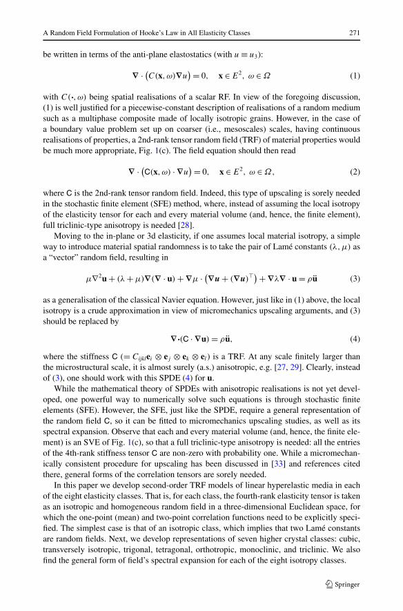
Regarding the modeling motivation (1), two basic issues are considered in this study:(i) type of anisotropy, and (ii) type of correlation structure. Now, with reference to Fig. 1
This material is based upon the research partially supported by the NSF under grants CMMI-1462749and IP-1362146 (I/UCRC on Novel High Voltage/Temperature Materials and Structures).
B A. [email protected]
1 Mälardalen University, Västerås, Sweden
2 University of Illinois at Urbana-Champaign, Urbana, IL, USA
270 A. Malyarenko, M. Ostoja-Starzewski
Fig. 1 (a) A realisation of a Voronoi tesselation (or mosaic); (b) placing a mesoscale window leads, viaupscaling, to a mesoscale random continuum approximation in (c)
showing a planar Voronoi tessellation of E2 which serves as a planar geometric model ofa polycrystal (although the same arguments apply in E3), each cell may be occupied by adifferently oriented crystal, with all the crystals belonging to any specific crystal class. Thelatter include:
– transverse isotropy modelling, say, sedimentary rocks at long wavelengths;– tetragonal modelling, say, wulfenite (PbMoO4);– trigonal modelling, say, dolomite (CaMg(CO3)2);– orthotropic, modelling, say, wood;– orthotropic modelling, say, orthoclase feldspar;– triclinic, modelling, say, microcline feldspar.
Thus, we need to be able to model 4th-rank tensor random fields, pointwise taking valuesin any crystal class. While the crystal orientations from grain to grain are random, theyare not spatially independent of each other—the assignment of crystal properties over thetessellation is not a white noise. This is precisely where the two-point characterisation of therandom field of elasticity tensor is needed. While the simplest correlation structure to admitwould be white-noise, a (much) more realistic model would account for any mathematicallyadmissible correlation structures as dictated by the statistically wide-sense homogeneousand isotropic assumption. A specific correlation can then be fitted to physical measurements.
Regarding the modeling motivation (1), it may also be of interest to work with amesoscale random continuum approximation defined by placing a mesoscale window atany spatial position as shown in Fig. 1(b). Clearly, the larger is the mesoscale window, theweaker are the random fluctuations in the mesoscale elasticity tensor: this is the trend tohomogenise the material when upscaling from a statistical volume element (SVE) to a rep-resentative volume element (RVE), e.g., [27, 30]. A simple paradigm of this upscaling, albeitonly in terms of a scalar random field, is the opacity of a sheet of paper held against light:the further away is the sheet from our eyes, the more homogeneous it appears. Similarly, inthe case of upscaling of elastic properties (which are tensor in character), on any finite scalethere is (almost surely) an anisotropy, and this anisotropy, with mesoscale increasing, tendsto zero hand-in-hand with the fluctuations. It is in the infinite mesoscale limit (i.e., RVE)that material isotropy is obtained as a consequence of the statistical isotropy.
Regarding the motivation (2) of this study, i.e., input of elasticity random fields intostochastic field equations, there are two principal routes: stochastic partial differential equa-tions (SPDE) and stochastic finite elements (SFE). The classical paradigm of SPDE [19] can
A Random Field Formulation of Hooke’s Law in All Elasticity Classes 271
be written in terms of the anti-plane elastostatics (with u ≡ u3):
∇ · (C(x,ω)∇u) = 0, x ∈ E2, ω ∈ Ω (1)
with C(·,ω) being spatial realisations of a scalar RF. In view of the foregoing discussion,(1) is well justified for a piecewise-constant description of realisations of a random mediumsuch as a multiphase composite made of locally isotropic grains. However, in the case ofa boundary value problem set up on coarser (i.e., mesoscales) scales, having continuousrealisations of properties, a 2nd-rank tensor random field (TRF) of material properties wouldbe much more appropriate, Fig. 1(c). The field equation should then read
∇ · (C(x,ω) · ∇u) = 0, x ∈ E2, ω ∈ Ω, (2)
where C is the 2nd-rank tensor random field. Indeed, this type of upscaling is sorely neededin the stochastic finite element (SFE) method, where, instead of assuming the local isotropyof the elasticity tensor for each and every material volume (and, hence, the finite element),full triclinic-type anisotropy is needed [28].
Moving to the in-plane or 3d elasticity, if one assumes local material isotropy, a simpleway to introduce material spatial randomness is to take the pair of Lamé constants (λ,μ) asa “vector” random field, resulting in
μ∇2u + (λ + μ)∇(∇ · u) + ∇μ · (∇u + (∇u)�) + ∇λ∇ · u = ρu (3)
as a generalisation of the classical Navier equation. However, just like in (1) above, the localisotropy is a crude approximation in view of micromechanics upscaling arguments, and (3)should be replaced by
∇·(C · ∇u) = ρu, (4)
where the stiffness C (= Cijklei ⊗ ej ⊗ ek ⊗ el) is a TRF. At any scale finitely larger thanthe microstructural scale, it is almost surely (a.s.) anisotropic, e.g. [27, 29]. Clearly, insteadof (3), one should work with this SPDE (4) for u.
While the mathematical theory of SPDEs with anisotropic realisations is not yet devel-oped, one powerful way to numerically solve such equations is through stochastic finiteelements (SFE). However, the SFE, just like the SPDE, require a general representation ofthe random field C, so it can be fitted to micromechanics upscaling studies, as well as itsspectral expansion. Observe that each and every material volume (and, hence, the finite ele-ment) is an SVE of Fig. 1(c), so that a full triclinic-type anisotropy is needed: all the entriesof the 4th-rank stiffness tensor C are non-zero with probability one. While a micromechan-ically consistent procedure for upscaling has been discussed in [33] and references citedthere, general forms of the correlation tensors are sorely needed.
In this paper we develop second-order TRF models of linear hyperelastic media in eachof the eight elasticity classes. That is, for each class, the fourth-rank elasticity tensor is takenas an isotropic and homogeneous random field in a three-dimensional Euclidean space, forwhich the one-point (mean) and two-point correlation functions need to be explicitly speci-fied. The simplest case is that of an isotropic class, which implies that two Lamé constantsare random fields. Next, we develop representations of seven higher crystal classes: cubic,transversely isotropic, trigonal, tetragonal, orthotropic, monoclinic, and triclinic. We alsofind the general form of field’s spectral expansion for each of the eight isotropy classes.
272 A. Malyarenko, M. Ostoja-Starzewski
2 The Formulation of the Problem
Let E = E3 be a three-dimensional Euclidean point space, and let V be the translation spaceof E with an inner product (·, ·). Following [35], the elements A of E are called the placesin E. The symbol B − A is the vector in V that translates A into B .
Let B ⊂ E be a deformable body. The strain tensor ε(A), A ∈ B, is a configurationvariable taking values in the symmetric tensor square S2(V ) of dimension 6. Following [25],we call this space a state tensor space.
The stress tensor σ(A) also takes values in S2(V ). This is a source variable, it describesthe source of a field [34].
We work with materials obeying Hooke’s law linking the configuration variable ε(A)
with the source variable σ(A) by
σ(A) = C(A)ε(A), A ∈ B.
Here the elastic modulus C is a linear map C(A) : S2(V ) → S2(V ). In linearised hy-perelasticity, the map C(A) is symmetric, i.e., an element of a constitutive tensor spaceV = S2(S2(V )) of dimension 21.
We assume that C(A) is a single realisation of a random field. In other words, denoteby B(V) the σ -field of Borel subsets of V. There is a probability space (Ω,F,P) and amapping C : B × Ω → V such that for any A0 ∈ B the mapping C(A0,ω) : Ω → V is(F,B(V))-measurable.
Translate the whole body B by a vector x ∈ V . The random fields C(A + x) and C(A)
have the same finite-dimensional distributions. It is therefore convenient to assume that thereis a random field defined on all of E such that its restriction to B is equal to C(A). Forbrevity, denote the new field by the same symbol C(A) (but this time A ∈ E). The randomfield C(A) is strictly homogeneous, that is, the random fields C(A + x) and C(A) have thesame finite-dimensional distributions. In other words, for each positive integer n, for eachx ∈ V , and for all distinct places A1, . . . , An ∈ E the random elements C(A1)⊕· · ·⊕ C(An)
and C(A1 + x)⊕· · ·⊕ C(An + x) of the direct sum on n copies of the space V have the sameprobability distribution.
Let K be the material symmetry group of the body B acting in V . The group K is asubgroup of the orthogonal group O(V ). Fix a place O ∈ B and identify E with V by themap f that maps A ∈ E to A − O ∈ V . Then K acts in E and rotates the body B by
g · A = f −1gfA, g ∈ K, A ∈ B.
Let A0 ∈ B. Under the above action of K the point A0 becomes g · A0. The random tensorC(A0) becomes S2(S2(g))C(A0). The random fields C(g ·A) and S2(S2(g))C(A) must havethe same finite-dimensional distributions, because g · A0 is the same material point in adifferent place. Note that this property does not depend on a particular choice of the place O ,because the field is strictly homogeneous.
To formalise the non-formal considerations of the above paragraph, note that the mapg → S2(S2(g)) is an orthogonal representation of the group K , that is, a continuous mapfrom K to the orthogonal group O(V) that respects the group operations:
S2(S2(g1g2)
) = S2(S2(g1)
)S2
(S2(g2)
), g1, g2 ∈ K.
Let U be an arbitrary orthogonal representation of the group K in a real finite-dimensionallinear space V with an inner product (·, ·), and let O be a place in E. A V-valued field C(A)
A Random Field Formulation of Hooke’s Law in All Elasticity Classes 273
is called strictly isotropic with respect to O if for any g ∈ K the random fields C(g · A) andU(g)C(A) have the same finite-dimensional distributions. If in addition the random fieldC(A) is strictly homogeneous, then it is strictly isotropic with respect to any place.
Assume that the random field C(A) is second-order, that is
E[‖C(A)‖2
]< ∞, A ∈ E.
Define the one-point correlation tensor of the field C(A) by⟨C(A)
⟩ = E[C(A)
]
and its two-point correlation tensor by⟨C(A),C(B)
⟩ = E[(
C(A) − ⟨C(A)
⟩) ⊗ (C(B) − ⟨
C(B)⟩)]
.
Assume that the field C(A) is mean-square continuous, that is, its two-point correlationtensor 〈C(A),C(B)〉 : E × E → V ⊗ V is a continuous function. If the field C(A) is strictlyhomogeneous, then its one-point correlation tensor is a constant tensor in V, while its two-point correlation tensor is a function of the vector B − A, i.e., a function on V . Call such afield wide-sense homogeneous.
Similarly, if the field C(A) is strictly isotropic, then we have⟨C(g · A)
⟩ = U(g)⟨C(A)
⟩,
⟨C(g · A),C(g · B)
⟩ = (U ⊗ U)(g)⟨C(A),C(B)
⟩.
Call such a field wide-sense isotropic. In what follows, we consider only wide-sense homo-geneous and isotropic random fields and omit the words “wide-sense”.
For simplicity, identify the field {C(A) : A ∈ E } defined on E with the field {C′(x) : x ∈V } defined by C′(x) = C(O + x). Introduce the Cartesian coordinate system (x, y, z) in V .Use the introduced system to identify V with the coordinate space R
3 and O(V ) with O(3).The action of O(3) on R
3 is the matrix-vector multiplication.Forte and Vianello [7] proved the existence of 8 symmetry classes of elasticity tensors,
or elasticity classes. In other words, consider the action
g · C = S2(S2(g)
)C
of the group K = O(3) in the space V = S2(S2(R3)). The symmetry group of an elasticitytensor C ∈ V is
K(C) = {g ∈ O(V ) : g · C = C
}.
Note that the symmetry group K(g · C) is conjugate through g to K(C):
K(g · C) = {ghg−1 : h ∈ K(C)
}. (5)
Whenever two bodies can be rotated so that their symmetry groups coincide, they share thesame symmetry class. Mathematically, two elasticity tensors C1 and C2 are equivalent ifand only if there is g ∈ O(3) such that K(C1) = K(g · C2). In view of (5), C1 and C2 areequivalent if and only if their symmetry groups are conjugate. The equivalence classes ofthe above relation are called the elasticity classes.
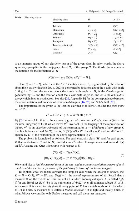
The first column of Table 1 adapted from [2], contains the name of an elasticity class.The second column represents a collection of subgroups H of O(3) such that H is conjugate
274 A. Malyarenko, M. Ostoja-Starzewski
Table 1 Elasticity classesElasticity class H N(H)
Triclinic Zc2 O(3)
Monoclinic Z2 × Zc2 O(2) × Zc
2Orthotropic D2 × Zc
2 O × Zc2
Trigonal D3 × Zc2 D6 × Zc
2Tetragonal D4 × Zc
2 D8 × Zc2
Transverse isotropic O(2) × Zc2 O(2) × Zc
2Cubic O × Zc
2 O × Zc2
Isotropic O(3) O(3)
to a symmetry group of any elasticity tensor of the given class. In other words, the abovesymmetry group lies in the conjugacy class [H ] of the group H . The third column containsthe notation for the normaliser N(H):
N(H) = {g ∈ O(3) : gHg−1 = H
}.
Here Zc2 = {I,−I }, where I is the 3 × 3 identity matrix, Zn is generated by the rotation
about the z-axis with angle 2π/n, O(2) is generated by rotations about the z-axis with angleθ , 0 ≤ θ < 2π and the rotation about the x-axis with angle π , Dn is the dihedral groupgenerated by Zn and the rotation about the x-axis with angle π , and O is the octahedralgroup which fixes an octahedron. See also [26, Appendix B] for the correspondence betweenthe above notation and notation of Hermann–Mauguin [16, 23] and Schönfließ [32].
The importance of the group N(H) can be clarified as follows. Consider the fixed pointset of H :
VH = {C ∈ V : g · C = C for all g ∈ H }.By [2, Lemma 3.1], if H is the symmetry group of some tensor C ∈ V, then N(H) is themaximal subgroup of O(3) which leaves VH invariant. In the language of the representationtheory, VH is an invariant subspace of the representation g → S2(S2(g)) of any group K
that lies between H and N(H), that is, S2(S2(g))C ∈ VH for all g ∈ K and for all C ∈ VH .Denote by U(g) the restriction of the above representation to VH .
The problem is formulated as follows. For each elasticity class [H ] and for each groupK that lies between H and N(H), consider an VH -valued homogeneous random field C(x)
on R3. Assume that C(x) is isotropic with respect to U :
⟨C(gx)
⟩ = U(g)⟨C(x)
⟩,
⟨C(gx),C(gy)
⟩ = (U ⊗ U)(g)⟨C(x),C(y)
⟩.
(6)
We would like to find the general form of the one- and two-point correlation tensors of sucha field and the spectral expansion of the field itself in terms of stochastic integrals.
To explain what we mean consider the simplest case when the answer is known. PutK = H = O(3), VH = R
1, and U(g) = 1, the trivial representation of K . Recall that ameasure Φ on the σ -field of Borel sets of a Hausdorff topological space X is called tightif for any Borel set B , Φ(B) is the supremum of Φ(K) over all compact subsets K of B .A measure Φ is called locally finite if every point of X has a neighbourhood U for whichΦ(U) is finite. A measure Φ is called a Radon measure if it is tight and locally finite. Inwhat follows we consider only Radon measures and call them just measures.
A Random Field Formulation of Hooke’s Law in All Elasticity Classes 275
Schoenberg [31] proved that the equation
⟨τ(x), τ (y)
⟩ =∫ ∞
0
sin(λ‖y − x‖)λ‖y − x‖ dΦ(λ)
establishes a one-to-one correspondence between the class of two-point correlation tensorsof homogeneous and isotropic random fields τ(x) and the class of finite measures on [0,∞).
Let L20(Ω) be the Hilbert space of centred complex-valued random variables with finite
variance. Let Z be a L20(Ω)-valued measure on the σ -field of Borel sets of a Hausdorff
topological space X. A measure Φ is called the control measure for Z, if for any Borel setsB1 and B2 we have
E[Z(B1)Z(B2)
] = Φ(B1 ∩ B2).
Yaglom [37] and independently M.I. Yadrenko in his unpublished PhD thesis proved thatthe field τ(x) has the form
τ(ρ, θ,ϕ) = C + π√
2∞∑
=0
∑
m=−
Sm (θ,ϕ)
∫ ∞
0
J +1/2(λρ)√λρ
dZm (λ),
where C = 〈τ(x)〉 ∈ R1, (ρ, θ,ϕ) are spherical coordinates in R
3, Sm (θ,ϕ) are real-valued
spherical harmonics, J +1/2(λρ) are the Bessel functions of the first kind of order + 1/2,and Zm
is a sequence of centred uncorrelated real-valued orthogonal random measures on[0,∞) with the measure Φ as their common control measure.
Other known results include the case of VH = R3, and U(g) = g. Yaglom [36] found
the general form of the two-point correlation tensor. Malyarenko and Ostoja-Starzewski[22] found the spectral expansion of the field. In the same paper, they found both the generalform of the two-point correlation tensor and the spectral expansion of the field for the case ofVH = S2(R3), and U(g) = S2(g). In [20] they solved one of the cases for two-dimensionalelasticity, when V = R
2, K = O(2), VH = S2(S2(R2)), and U(g) = S2(S2(g)).
Remark 1 Another approach to studying tensor-valued random fields was elaborated byGuilleminot and Soize [11–15]. Using a stochastic model alternative to our model, theyconstructed a generator for random fields that have prescribed symmetry properties, takevalues in the set of symmetric nonnegative-definite tensors, depend on a few real parameters,and may be easily simulated and calibrated. The question of constructing a generator withsimilar properties based on the stochastic model described below raises several interestingissues and will be considered in forthcoming publications.
3 A General Result
The idea of this Section is as follows. Let V be a finite-dimensional real linear space, let K
be a closed subgroup of the group O(3), and let U be an orthogonal representation of thegroup K in the space V. Consider a homogeneous and isotropic random field C(x), x ∈ R
3,and solve the problem formulated in Section 2. In Section 5, apply general formulae to ourcases. The resulting Theorems 1–16 are particular cases of general Theorem 0.
To obtain general formulae, we describe all homogeneous random fields taking values inV and throw away non-isotropic ones. The first obstacle here is as follows. The completedescription of such fields is unknown. We use the following result instead.
276 A. Malyarenko, M. Ostoja-Starzewski
Let VC be a complex finite-dimensional linear space with an inner product (·, ·) that islinear in the second argument, as is usual in physics. Let J be a real structure on VC, that is,a map J : VC → VC satisfying the following conditions:
J (αC1 + βC2) = αJ (C1) + βJ (C2),
J(J (C)
) = C
for all α, β ∈ C and for all C1, C2 ∈ VC. In other words, J is a multidimensional andcoordinate-free generalisation of complex conjugation. The set of all eigenvectors of J thatcorrespond to eigenvalue 1, constitute a real linear space, denote it by V. Let H be the reallinear space of Hermitian linear operators in VC. The real structure J induces a linear oper-ator J in H. For any A ∈ H, the operator JA acts by
(JA)C = J (AJC), C ∈ VC.
In coordinates, the operator J is just the transposition of a matrix.The result by Cramér [5] in coordinate-free form is formulated as follows. Equation
⟨C(x),C(y)
⟩ =∫
R3ei(p,y−x) dF(p) (7)
establishes a one-to-one correspondence between the class of two-point correlation tensorsof homogeneous mean-square continuous VC-valued random fields C(x) and the class ofmeasures on the σ -field of Borel sets of the wavenumber domain R
3 tasking values in theset of nonnegative-definite Hermitian linear operators in VC. For V-valued random fields,there is only a necessary condition: if C(x) is V-valued, then the measure F satisfies
F(−B) = JF(B), B ∈B(R
3),
where −B = {−p : p ∈ B }.Introduce the trace measure μ by μ(B) = trF(B), B ∈ B(R3) and note that F is abso-
lutely continuous with respect to μ. This means that (7) may be written as
⟨C(x),C(y)
⟩ =∫
R3ei(p,y−x)f (p)dμ(p),
where f (p) is a measurable function on the wavenumber domain taking values in the setof all nonnegative-definite Hermitian linear operators in VC with unit trace, that satisfies thefollowing condition
f (−p) = Jf (p). (8)
Using representation theory, it is possible to prove the following. Let C1, C2 ∈ V. LetL(C1 ⊗ C2) be the operator in H acting on a tensor C ∈ VC by
L(C1 ⊗ C2)C = (JC1,C)C2.
By linearity, this action may be extended to an isomorphism L between V ⊗ V and H. Theorthogonal operators LU ⊗ U(g)L−1, g ∈ K , constitute an orthogonal representation of thegroup K in the space H, equivalent to the tensor square U ⊗ U of the representation U . Theoperator L is an intertwining operator between the spaces V ⊗ V and H where equivalent
A Random Field Formulation of Hooke’s Law in All Elasticity Classes 277
representations U ⊗ U and LU ⊗ UL−1 act. In what follows, we are working only withthe latter representation, for simplicity denote it again by U ⊗ U and note that it acts in thespace H by
(U ⊗ U)(g)A = U(g)AU−1(g), A ∈ H.
Denote H+ = LS2(V). In coordinates, it is the subspace of Hermitian matrices with real-valued matrix entries. If −I ∈ K , then the second equation in (6) and (8) together are equiv-alent to the following conditions:
μ(gB) = μ(B), B ∈ B(R
3)
(9)
and
f (p) ∈ H+, f (gp) = S2(U(g)
)f (p). (10)
The description of all measures μ satisfying (9) is well known, see [3]. There are finitelymany, say M , orbit types for the action of K in R
3 by
(gp,x) = (p, g−1x
).
Denote by (R3/K)m, 0 ≤ m ≤ M − 1 the set of all orbits of the mth type. It is known,see [2], that all the above sets are manifolds. Assume for simplicity of notation that thereare charts λm such that the domain of λm is dense in (R3/K)m. The orbit of the mth type isthe manifold K/Hm, where Hm is a stationary subgroup of a point on the orbit. Assume thatthe domain of a chart ϕm is a dense set in K/Hm, and let dϕm be the unique probabilisticK-invariant measure on the σ -field of Borel sets of K/Hm. There are the unique measuresΦm on the σ -fields of Borel sets in (R3/K)m such that
∫
R3ei(p,y−x)f (p)dμ(p) =
M−1∑
m=0
∫
(R3/K)m
∫
K/Hm
ei((λm,ϕm),y−x)f (λm,ϕm)dϕm dΦm(λm).
To find all functions f satisfying (10), proceed as follows. Fix an orbit λm and denoteby ϕ0
m the coordinates of the intersection of the orbit λm with the set (R3/K)m. Let Um bethe restriction of the representation S2(U) to the group Hm. We have g(λm,ϕ0
m) = (λm,ϕ0m)
for all g ∈ Hm, because Hm is the stationary subgroup of the point (λm,ϕ0m). For g ∈ Hm,
(10) becomes
f(λm,ϕ0
m
) = Um(g)f(λm,ϕ0
m
). (11)
Any orthogonal representation of a compact topological group in a space H has at leasttwo invariant subspaces: {0} and H. The representation is called irreducible if no other invari-ant subspaces exist. The space of any finite-dimensional orthogonal representation of a com-pact topological group can be uniquely decomposed into a direct sum of isotypic subspaces.Each isotypic subspace is the direct sum of finitely many subspaces where the copies of thesame irreducible representation act. Equation (11) means that the operator f (λm,ϕ0
m) liesin the isotypic subspace Hm which corresponds to the trivial representation of the group Hm.The intersection of this subspace with the convex compact set of all nonnegative-definiteoperators in H+ with unit trace is again a convex compact set, call it Cm. As λm runs over(R3/K)m, f (λm,ϕ0
m) becomes an arbitrary measurable function taking values in Cm.An irreducible orthogonal representation of the group K is called a representation of
class 1 with respect to the group Hm if the restriction of this representation to Hm con-tains at least one copy of the trivial representation of Hm. Let S2(U)m be the restriction
278 A. Malyarenko, M. Ostoja-Starzewski
of the representation S2(U) to the direct sum of the isotypic subspaces of the irreduciblerepresentation of class 1 with respect to Hm. Let gϕm
be an arbitrary element of K suchthat gϕm
(ϕ0m) = ϕm. Two such elements differ by an element of Hm, therefore the second
equation in (10) becomes
f (λm,ϕm) = S2(U(gϕm
))mf
(λm,ϕ0
m
).
The two-point correlation tensor of the field takes the form
⟨C(x),C(y)
⟩ =M−1∑
m=0
∫
(R3/K)m
∫
K/Hm
ei(gϕm(λm,ϕ0m),y−x)S2
(U(gϕm
))m
× f(λm,ϕ0
m
)dϕm dΦm(λm). (12)
Choose an orthonormal basis T1, . . . ,Tdim V in the space V. The tensor square V ⊗ V hasseveral orthonormal bases. The coupled basis consists of tensor products Ti ⊗ Tj , 1 ≤ i,j ≤ dim V. The mth uncoupled basis is build as follows. Let Um,1, . . . ,Um,km be all non-equivalent irreducible orthogonal representations of the group K of class 1 with respect toHm such that the representation S2(U) contains isotypic subspaces where cmk copies of therepresentation Um,k act, and let the restriction of the representation Um,k to Hm containsdmk copies of the trivial representation of Hm. Let Tmkln, 1 ≤ l ≤ dmk , 1 ≤ n ≤ cmk be anorthonormal basis in the space where the nth copy act. Complete the above basis to thebasis Tmkln, 1 ≤ l ≤ dimUm,k and call this basis the mth uncoupled basis. The vectors of thecoupled basis are linear combinations of the vectors of the mth uncoupled basis:
Ti ⊗ Tj =km∑
k=1
dimUm,k∑
l=1
cmk∑
n=1
cmklnij Tmkln + · · · ,
where dots denote the terms that include the tensors in the basis of the space S2(V)�S2(V)m.In the introduced coordinates, (12) takes the form
⟨C(x),C(y)
⟩ij
=M−1∑
m=0
km∑
k=1
dimUm,k∑
l=1
dmk∑
l′=1
cmk∑
n=1
cmklnij
∫
(R3/K)m
∫
K/Hm
ei(gϕm(λm,ϕ0m),y−x)
× Um,k
ll′ (ϕm)fl′n(λm,ϕ0
m
)dϕm dΦm(λm). (13)
The choice of bases inside the isotypic subspaces is not unique. One has to choose them insuch a way that calculation of the transition coefficients cmkln
ij is as easy as possible.To calculate the inner integrals, we proceed as follows. Consider the action of K on R
3
by matrix-vector multiplication. Let (R3/K)m, 0 ≤ m ≤ M − 1 be the set of all orbits ofthe mth type. Let ρm be such a chart that its domain is dense in (R3/K)m. Let ψm be achart in K/Hm with a dense domain, and let dψm be the unique probabilistic K-invariantmeasure on the σ -field of Borel sets of K/Hm. It is known that the sets of orbits of one ofthe types, say (R3/K)M−1 (resp. (R3/K)M−1), are dense in R
3 (resp. R3). Write the plane
wave ei(gϕM−1 (λM−1,ϕ0M−1),y−x) as
ei(gϕM−1 (λM−1,ϕ0M−1),y−x) = ei(gϕM−1 (λM−1,ϕ0
M−1),gψM−1(ρM−1,ψ0
M−1)),
A Random Field Formulation of Hooke’s Law in All Elasticity Classes 279
and consider the plane wave as a function of two variables ϕM−1 and ψM−1 with domain(K/HM−1)
2. This function is K-invariant:
ei(ggϕM−1 (λM−1,ϕ0M−1),ggψM−1
(ρM−1,ψ0M−1)) = ei(gϕM−1 (λM−1,ϕ0
M−1),gψM−1(ρM−1,ψ0
M−1)), g ∈ K.
Denote by KHM−1 the set of all equivalence classes of irreducible representations of K of
class 1 with respect to HM−1, and let the restriction of the representation Uq ∈ KHM−1 toHM−1 contains dq copies of the trivial representation of HM−1. By the Fine Structure Theo-rem [17], there are some numbers d ′
q ≤ dq such that the set
{dimUq · Uq
ll′(ϕM−1)Uq
ll′(ψM−1) : Uq ∈ KHM−1 ,1 ≤ l ≤ dimUq,1 ≤ l′ ≤ d ′q
}
is the orthonormal basis in the Hilbert space L2((K/HM−1)2,dϕM−1 dψM−1). Let
jq
ll′(λM−1,ρM−1) = dimUq
∫
(K/HM−1)2ei(gϕM−1 (λM−1,ϕ0
M−1),gψM−1(ρM−1,ψ0
M−1))
× Uq
ll′(ϕM−1)Uq
ll′(ψM−1)dϕM−1 dψM−1
be the corresponding Fourier coefficients. The uniformly convergent Fourier expansion takesthe form
ei(gϕM−1 (λM−1,ϕ0M−1),gψM−1
(ρM−1,ψ0M−1)) =
∑
Uq∈KHM−1
dimUq∑
l=1
d ′q∑
l′=1
dimUq
× jq
ll′(λM−1,ρM−1)Uq
ll′(ϕM−1)Uq
ll′(ψM−1).
(14)
This expansion is defined on the dense set
(R
3/K)M−1
× (K/HM−1) × (R
3/K)M−1
× (K/HM−1)
and may be extended to all of R3 × R3 by continuity. Substituting the extended expansion
to (13), we obtain the expansion
⟨C(x),C(y)
⟩ij
=M−1∑
m=0
km∑
k=1
dimUm,k∑
l=1
d ′mk∑
l′=1
cmk∑
n=1
cmklnij
∫
(R3/K)m
jq
ll′(λm,ρ0)
× Um,k
ll′ (ψm)fl′n(λm,ϕ0
m
)dΦm(λm). (15)
Theorem 0 Let −I ∈ K . The one-point correlation tensor of a homogeneous and (K,U)-isotropic random field lies in the space of the isotypic component of the representation U
that corresponds to the trivial representation of K and is equal to 0 if no such isotypiccomponent exists. Its two-point correlation tensor is given by (15).
Remark 2 The results by [20, 22, 31, 36, 37] as well as Theorems 1–16 below are particularcases of Theorem 0. The expansion (15) is the first necessary step in studying random fieldsconnected to Hooke’s law.
280 A. Malyarenko, M. Ostoja-Starzewski
Later we will see that it is easy to write the spectral expansion of the field directly ifthe group K is finite. Otherwise, we write the Fourier expansion (14) for plane waves ei(p,y)
and e−i(p,x) separately and substitute both expansions to (13). As a result, we obtain theexpansion of the two-point correlation tensor of the field in the form
⟨C(x),C(y)
⟩ij
=∫
Λ
u(x, λ)u(y, λ)dΦij (λ),
where Λ is a set, and where F is a measure on a σ -field L of subsets of Λ taking values in theset of Hermitian nonnegative-definite operators on VC. Moreover, the set {u(x, λ) : x ∈ R
3 }is total in the Hilbert space L2(Λ,Φ) of the measurable complex-valued functions on Λ
that are square-integrable with respect to the measure Φ , that is, the set of finite linearcombinations
∑cnu(xn, λ) is dense in the above space. By Karhunen’s theorem [18], the
field C(x) has the following spectral expansion:
C(x) = E[C(0)
] +∫
Λ
u(x, λ)dZ(λ), (16)
where Z is a measure on the measurable space (Λ,L) taking values in the Hilbert space ofrandom tensors Z : Ω → VC with E[Z] = 0 and E[‖Z‖2] < ∞. The measure F is the controlmeasure of the measure Z, i.e.,
E[JZ(A)Z�(B)
] = Φ(A ∩ B), A,B ∈ L.
The components of the random tensor Z(A) are correlated, which creates difficulties whenone tries to use (16) for computer simulation. It is possible to use Cholesky decompositionand to write the expansion of the field using uncorrelated random measures, see detailsin [22].
4 Preliminary Calculations
The possibilities for the group K are as follows. In the triclinic class, there exist infinitelymany groups between Zc
2 and O(3), we put K1 = Zc2 and K2 = O(3). Similarly, for the
monoclinic class put K3 = Z2 ×Zc2 and K4 = O(2)×Zc
2. The possibilities for the orthotropicclass are K5 = D2 × Zc
2, K6 = D4 × Zc2, K7 = D6 × Zc
2, K8 = T × Zc2, and K9 = O × Zc
2.Here T is the tetrahedral group which fixes a tetrahedron. In the trigonal class, we haveK10 = D3 × Zc
2 and K11 = D6 × Zc2. In the tetragonal class, the possibilities are K12 =
D4 × Zc2 and K13 = D8 × Zc
2. In the three remaining classes, the possibilities are K14 =O(2)×Zc
2, K15 = O ×Zc2, and K16 = O(3). The intermediate groups were determined using
[4, Vol. 1, Fig. 10.1.3.2]. For each group Ki , 1 ≤ i ≤ 16, we formulate Theorem number i
below.
4.1 The Structure of the Representation U
The notation for irreducible orthogonal representation is as follows. If Ki is a finite group,we use the Mulliken notation [24], see also [1, Chapter 14] to denote the irreducible unitaryrepresentation of Ki . For an irreducible orthogonal representation, consider its complexifi-cation. A standard result of representation theory, see, for example, [6, Proposition 4.8.4],states that there are three possibilities:
A Random Field Formulation of Hooke’s Law in All Elasticity Classes 281
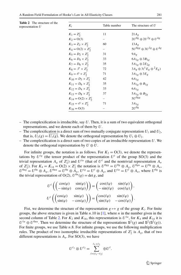
Table 2 The structure of therepresentation U Ki Table number The structure of U
K1 = Zc2 11 21Ag
K2 = O(3) – 2U0g ⊕ 2U2g ⊕ U4g
K3 = Z2 × Zc2 60 13Ag
K4 = O(2) × Zc2 – 5U0gg ⊕ 3U2g ⊕ U4g
K5 = D2 × Zc2 31 9Ag
K6 = D4 × Zc2 33 6A1g ⊕ 3B1g
K7 = D6 × Zc2 35 5A1g ⊕ 2E2g
K8 = T × Zc2 72 3Ag ⊕ 3(1Eg ⊕ 2Eg)
K9 = O × Zc2 71 3A1g ⊕ 3Eg
K10 = D3 × Zc2 42 6A1g
K11 = D6 × Zc2 35 5A1g ⊕ B1g
K12 = D4 × Zc2 33 6A1g
K13 = D8 × Zc2 37 5A1g ⊕ B2g
K14 = O(2) × Zc2 – 5U0gg
K15 = O × Zc2 71 3A1g
K16 = O(3) – 2U0g
– The complexification is irreducible, say U . Then, it is a sum of two equivalent orthogonalrepresentations, and we denote each of them by U .
– The complexification is a direct sum of two mutually conjugate representation U1 and U2,that is, U2(g) = U1(g). We denote the orthogonal representation by U1 ⊕ U2.
– The complexification is a direct sum of two copies of an irreducible representation U . Wedenote the orthogonal representation by U ⊕ U .
For infinite groups, the notation is as follows. For K2 = O(3), we denote the represen-tations by U g (the tensor product of the representation U of the group SO(3) and thetrivial representation Ag of Zc
2) and U u (that of U and the nontrivial representation Au
of Zc2). For K4 = K14 = O(2) × Zc
2 the notation is U 0gg = U 0g ⊗ Ag , U 0gu = U 0g ⊗ Au,U 0ug = U 0u ⊗ Ag , U 0uu = U 0u ⊗ Au, U g = U ⊗ Ag , and U u = U ⊗ Au, where U 0g isthe trivial representation of O(2), U 0u(g) = detg, and
U
((cos(ϕ) sin(ϕ)
− sin(ϕ) cos(ϕ)
))=
(cos( ϕ) sin( ϕ)
− sin( ϕ) cos( ϕ)
),
U
((cos(ϕ) sin(ϕ)
sin(ϕ) − cos(ϕ)
))=
(cos( ϕ) sin( ϕ)
sin( ϕ) − cos( ϕ)
).
Fist, we determine the structure of the representation g → g of the group Ki . For finitegroups, the above structure is given in Table n.10 in [1], where n in the number given in thesecond column of Table 2. For K2 and K16, this representation is U 1u, for K4 and K14 it isU 1u ⊕ U 0uu. Then we determine the structure of the representations S2(g) and S2(S2(g)).For finite groups, we use Table n.8. For infinite groups, we use the following multiplicationrules. The product of two isomorphic irreducible representations of Zc
2 is Ag , that of twodifferent representations is Au. For SO(3), we have
U 1 ⊗ U 2 = 1+ 2∑
=| 1− 2|⊕U .
282 A. Malyarenko, M. Ostoja-Starzewski
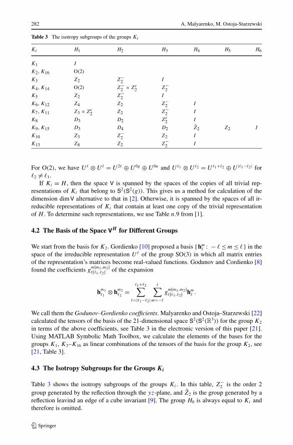
Table 3 The isotropy subgroups of the groups Ki
Ki H1 H2 H3 H4 H5 H6
K1 I
K2, K16 O(2)
K3 Z2 Z−2 I
K4, K14 O(2) Z−2 × Zc
2 Z−2
K5 Z2 Z−2 I
K6, K12 Z4 Z2 Z−2 I
K7, K11 Z3 × Zc2 Z2 Z−
2 I
K8 D3 D2 Zc2 I
K9, K15 D3 D4 D2 Z2 Z2 I
K10 Z3 Z−2 Z2 I
K13 Z8 Z2 Z−2 I
For O(2), we have U ⊗ U = U 2 ⊕ U 0g ⊕ U 0u and U 1 ⊗ U 2 = U 1+ 2 ⊕ U | 1− 2| for 2 �= 1.
If Ki = H , then the space V is spanned by the spaces of the copies of all trivial rep-resentations of Ki that belong to S2(S2(g)). This gives us a method for calculation of thedimension dim V alternative to that in [2]. Otherwise, it is spanned by the spaces of all ir-reducible representations of Ki that contain at least one copy of the trivial representationof H . To determine such representations, we use Table n.9 from [1].
4.2 The Basis of the Space VH for Different Groups
We start from the basis for K2. Gordienko [10] proposed a basis {hm : − ≤ m ≤ } in the
space of the irreducible representation U of the group SO(3) in which all matrix entriesof the representation’s matrices become real-valued functions. Godunov and Cordienko [8]found the coefficients g
m[m1,m2] [ 1, 2] of the expansion
hm1 1
⊗ hm2 2
= 1+ 2∑
=| 1− 2|
∑
m=−
gm[m1,m2] [ 1, 2] hm
.
We call them the Godunov–Gordienko coefficients. Malyarenko and Ostoja–Starzewski [22]calculated the tensors of the basis of the 21-dimensional space S2(S2(R3)) for the group K2
in terms of the above coefficients, see Table 3 in the electronic version of this paper [21].Using MATLAB Symbolic Math Toolbox, we calculate the elements of the bases for thegroups K1, K3–K16 as linear combinations of the tensors of the basis for the group K2, see[21, Table 3].
4.3 The Isotropy Subgroups for the Groups Ki
Table 3 shows the isotropy subgroups of the groups Ki . In this table, Z−2 is the order 2
group generated by the reflection through the yz-plane, and Z2 is the group generated by areflection leavind an edge of a cube invariant [9]. The group H0 is always equal to Ki andtherefore is omitted.
A Random Field Formulation of Hooke’s Law in All Elasticity Classes 283
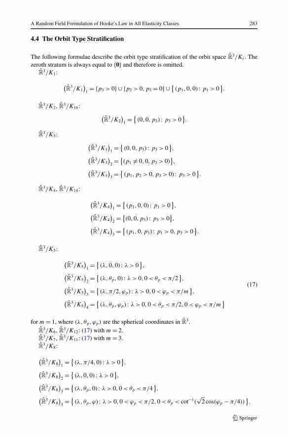
4.4 The Orbit Type Stratification
The following formulae describe the orbit type stratification of the orbit space R3/Ki . The
zeroth stratum is always equal to {0} and therefore is omitted.R
3/K1:
(R
3/K1
)1= {p3 > 0} ∪ {p2 > 0,p3 = 0} ∪ {
(p1,0,0) : p1 > 0}.
R3/K2, R3/K16:
(R
3/K2
)1= {
(0,0,p3) : p3 > 0}.
R3/K3:
(R
3/K3)
1= {
(0,0,p3) : p3 > 0},
(R
3/K3
)2= {
(p1 �= 0,0,p3 > 0)},
(R
3/K3
)3= {
(p1,p2 > 0,p3 > 0) : p3 > 0}.
R3/K4, R3/K14:
(R
3/K4
)1= {
(p1,0,0) : p1 > 0},
(R
3/K4
)2= {
(0,0,p3) : p3 > 0},
(R
3/K4)
3= {
(p1,0,p3) : p1 > 0,p3 > 0}.
R3/K5:
(R
3/K5
)1= {
(λ,0,0) : λ > 0},
(R
3/K5
)2= {
(λ, θp,0) : λ > 0,0 < θp < π/2},
(R
3/K5
)3= {
(λ,π/2, ϕp) : λ > 0,0 < ϕp < π/m},
(R
3/K5)
4= {
(λ, θp,ϕp) : λ > 0,0 < θp < π/2,0 < ϕp < π/m}
(17)
for m = 1, where (λ, θp,ϕp) are the spherical coordinates in R3.
R3/K6, R3/K12: (17) with m = 2.
R3/K7, R3/K11: (17) with m = 3.
R3/K8:
(R
3/K8
)1= {
(λ,π/4,0) : λ > 0},
(R
3/K8)
2= {
(λ,0,0) : λ > 0},
(R
3/K8
)3= {
(λ, θp,0) : λ > 0,0 < θp < π/4},
(R
3/K8
)3= {
(λ, θp,ϕ) : λ > 0,0 < ϕp < π/2,0 < θp < cot−1(√
2 cos(ϕp − π/4))}.
284 A. Malyarenko, M. Ostoja-Starzewski
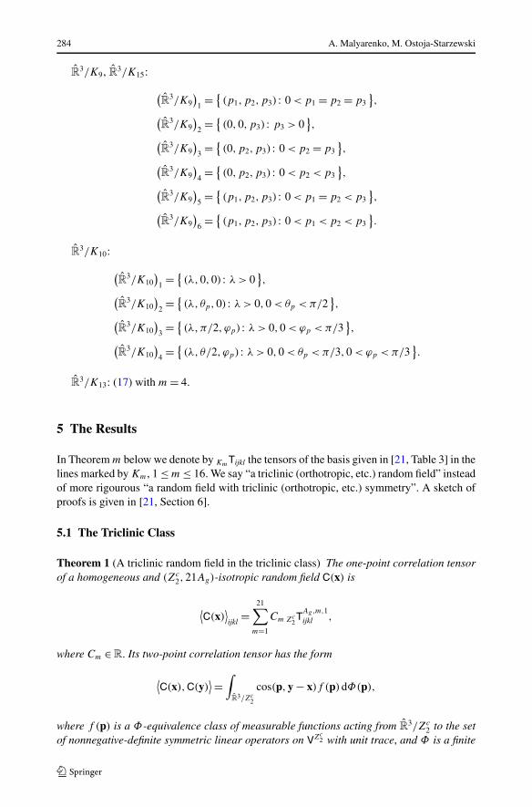
R3/K9, R3/K15:
(R
3/K9
)1= {
(p1,p2,p3) : 0 < p1 = p2 = p3
},
(R
3/K9
)2= {
(0,0,p3) : p3 > 0},
(R
3/K9)
3= {
(0,p2,p3) : 0 < p2 = p3},
(R
3/K9
)4= {
(0,p2,p3) : 0 < p2 < p3
},
(R
3/K9
)5= {
(p1,p2,p3) : 0 < p1 = p2 < p3
},
(R
3/K9)
6= {
(p1,p2,p3) : 0 < p1 < p2 < p3}.
R3/K10:
(R
3/K10)
1= {
(λ,0,0) : λ > 0},
(R
3/K10
)2= {
(λ, θp,0) : λ > 0,0 < θp < π/2},
(R
3/K10
)3= {
(λ,π/2, ϕp) : λ > 0,0 < ϕp < π/3},
(R
3/K10)
4= {
(λ, θ/2, ϕp) : λ > 0,0 < θp < π/3,0 < ϕp < π/3}.
R3/K13: (17) with m = 4.
5 The Results
In Theorem m below we denote by KmTijkl the tensors of the basis given in [21, Table 3] in thelines marked by Km, 1 ≤ m ≤ 16. We say “a triclinic (orthotropic, etc.) random field” insteadof more rigourous “a random field with triclinic (orthotropic, etc.) symmetry”. A sketch ofproofs is given in [21, Section 6].
5.1 The Triclinic Class
Theorem 1 (A triclinic random field in the triclinic class) The one-point correlation tensorof a homogeneous and (Zc
2,21Ag)-isotropic random field C(x) is
⟨C(x)
⟩ijkl
=21∑
m=1
Cm Zc2T
Ag,m,1ijkl ,
where Cm ∈R. Its two-point correlation tensor has the form
⟨C(x),C(y)
⟩ =∫
R3/Zc2
cos(p,y − x)f (p)dΦ(p),
where f (p) is a Φ-equivalence class of measurable functions acting from R3/Zc
2 to the setof nonnegative-definite symmetric linear operators on VZc
2 with unit trace, and Φ is a finite
A Random Field Formulation of Hooke’s Law in All Elasticity Classes 285
measure on R3/Zc
2. The field has the form
Cijkl(x) =21∑
m=1
Cm Zc2T
Ag,m,1ijkl +
21∑
m=1
∫
R3/Zc2
cos(p,x)dZ1m(p)Zc
2T
Ag,m,1ijkl
+21∑
m=1
∫
R3/Zc2
sin(p,x)dZ2m(p)Zc
2T
Ag,m,1ijkl ,
where (Zm1 (p), . . . ,Zm
21(p))� are two centred uncorrelated VZc2 -valued random measures on
R3/Zc
2 with control measure f (p)dΦ(p).
Theorem 2 (An isotropic random field in the triclinic class) The one-point correlation ten-sor of a homogeneous and (O(3),2U 0g ⊕ 2U 2g ⊕ U 4g)-isotropic random field C(x) is
⟨C(x)
⟩ijkl
= C1TU0g,1,1ijkl + C2TU0g,2,1
ijkl ,
where C1, C2 ∈R. Its two-point correlation tensor has the spectral expansion
⟨C(x),C(y)
⟩ijkli′j ′k′l′ =
3∑
n=1
∫ ∞
0
29∑
q=1
Nnq(λ,ρ)Lq
iikli′j ′k′l′(y − x)dΦn(λ).
The measures Φn(λ) satisfy the condition
Φ2
({0}) = 2Φ3
({0}).The spectral expansion of the field has the form
Cijkl(ρ, θ,ϕ) = C1TU0g,1,1ijkl + C2TU0g,2,1
ijkl
+ 2√
π
13∑
m=1
∞∑
t=0
t∑
u=−t
∫ ∞
0jt (λρ)dZmtuijkl(λ)Su
t (θ, ϕ),
where Sut (θ, ϕ) are real-valued spherical harmonics.
The functions Nnq(λ,ρ) and Lq
iikli′j ′k′l′(y − x) are given in [21, Tables 5, 6].
5.2 The Monoclinic Class
Theorem 3 (A monoclinic random field in the monoclinic class) The one-point correlationtensor of a homogeneous and (Z2 × Zc
2,13Ag)-isotropic random field C(x) is
⟨C(x)
⟩ijkl
=13∑
m=1
Cm Z2×Zc2T
Ag,m,1ijkl ,
where Cm ∈R. Its two-point correlation tensor has the form
⟨C(x),C(y)
⟩ = 1
2
∫
R3/Z2×Zc2
cos(p1(y1 − x1) + p2(y2 − x2)
)cos
(p3(y3 − x3)
)f (p)dΦ(p),
286 A. Malyarenko, M. Ostoja-Starzewski
where f (p) is a Φ-equivalence class of measurable functions acting from R3/Z2 × Zc
2 tothe set of nonnegative-definite symmetric linear operators on VZ2×Zc
2 with unit trace, and Φ
is a finite Radon measure on R3/Z2 × Zc
2. The field has the form
C(x)ijkl =13∑
m=1
Cm Z2×Zc2T
Ag,m,1ijkl
+ 1√2
13∑
m=1
∫
R3/Z2×Zc2
cos(p1x + p2y) cos(p3z)dZ1m(p)Z2×Zc
2T
Ag,m,1ijkl
+ 1√2
13∑
m=1
∫
R3/Z2×Zc2
sin(p1x + p2y) sin(p3z)dZ2m(p)Z2×Zc
2T
Ag,m,1ijkl
+ 1√2
13∑
m=1
∫
R3/Z2×Zc2
cos(p1x + p2y) sin(p3z)dZ3m(p)Z2×Zc
2T
Ag,m,1ijkl
+ 1√2
13∑
m=1
∫
R3/Z2×Zc2
sin(p1x + p2y) cos(p3z)dZ4m(p)Z2×Zc
2T
Ag,m,1ijkl ,
where (Zn1 (p), . . . ,Zn
13(p))� are four centred uncorrelated VZ2×Zc2 -valued random measures
on R3/Z2 × Zc
2 with control measure f (p)dΦ(p).
Theorem 4 (A transverse isotropic random field in the monoclinic class) The one-point cor-relation tensor of a homogeneous and (O(2) × Zc
2,5U 0gg ⊕ 3U 2g ⊕ U 4g)-isotropic randomfield C(x) is
⟨C(x)
⟩ijkl
=5∑
m=1
Cm O(2)×Zc2TU0gg,m,1
ijkl ,
where Cm ∈R. Its two-point correlation tensor has the form
⟨C(x),C(y)
⟩ =∫
R3/O(2)×Zc2
J0
(√(p2
1 + p22
)(z2
1 + z22
))cos(p3z3)f (p)dΦ(p),
where Φ is a measure on R3/O(2) × Zc
2, and f (p) is a Φ-equivalence class of measurablefunctions on R
3/O(2) × Zc2 with values in the compact set of all nonnegative-definite linear
operators in the space VO(2)×Zc2 with unit trace of the form
⎛
⎜⎜⎜⎜⎝
A 0 0 0 00 B1 B2 B3 00 B2 B4 B5 00 B3 B5 B6 00 0 0 0 B7
⎞
⎟⎟⎟⎟⎠
,
A Random Field Formulation of Hooke’s Law in All Elasticity Classes 287
where A is a nonnegative-definite 5 × 5 matrix, and Bm, 1 ≤ m ≤ 7 are 2 × 2 matricesproportional to the identity matrix. The field has the form
C(x) =5∑
m=1
CmTmijkl
+13∑
m=1
∫
R3/O(2)×Zc2
J0
(√(p2
1 + p22
)(z2
1 + z22
))
× (cos(p3z)dZ01
m (p)Tmijkl + sin(p3z)dZ02
m (p)Tmijkl
)
+ √2
∞∑
=1
13∑
m=1
∫
R3/O(2)×Zc2
J
(√(p2
1 + p22
)(z2
1 + z22
))
× (cos(p3z) cos( ϕp)dZ 1
m (p)Tmijkl + cos(p3z) sin( ϕp)dZ 2m(p)Tm
ijkl
+ sin(p3z) cos( ϕp)dZ 3m (p)Tm
ijkl + sin(p3z) sin( ϕp)dZ 4m (p)Tm
ijkl
),
where (Z i1 (p), . . . ,Z i
13(p))� are centred uncorrelated VO(2)×Zc2 -valued random measures on
R3/O(2) × Zc
2 with control measure f (p)dΦ(p), and
Tmijkl =
⎧⎪⎨
⎪⎩
O(2)×Zc2TU0gg,m,1, if 1 ≤ m ≤ 5,
O(2)×Zc2TU2g,�m/2�−2,m mod 2+1, if 6 ≤ m ≤ 11,
O(2)×Zc2TU4g,1,m−11, if 12 ≤ m ≤ 13.
5.3 The Orthotropic Class
Theorem 5 (An orthotropic random field in the orthotropic class) The one-point correlationtensor of a homogeneous and (D2 × Zc
2,9Ag)-isotropic random field C(x) is
⟨C(x)
⟩ijkl
=9∑
m=1
Cm D2×Zc2T
Ag,m,1ijkl ,
where Cm ∈R. Its two-point correlation tensor has the form
⟨C(x),C(y)
⟩ =∫
R3/D2×Zc2
cos(p1(y1 − x1)
)cos
(p2(y2 − x2)
)cos
(p3(y3 − x3)
)f (p)dΦ(p),
where f (p) is a Φ-equivalence class of measurable functions acting from R3/D2 × Zc
2 tothe set of nonnegative-definite symmetric linear operators on VD2×Zc
2 with unit trace, and Φ
is a finite measure on R3/D2 × Zc
2. The field has the form
C(x)ijkl =9∑
m=1
Cm D2×Zc2T
Ag,m,1ijkl +
9∑
m=1
8∑
n=1
∫
R3/D2×Zc2
un(p,x)dZnm(p)D2×Zc
2T
Ag,m,1ijkl ,
where (Zn1 (p), . . . ,Zn
9 (p))� are eight centred uncorrelated VD2×Zc2 -valued random measures
on R3/D2 × Zc
2 with control measure f (p)dΦ(p), and where un(p,x) are eight differentproduct of sines and cosines of prxr .
288 A. Malyarenko, M. Ostoja-Starzewski
Consider a 9×9 symmetric nonnegative-definite matrix with the unit trace of the follow-ing structure:
(A B
B� C
),
where A is a 6 × 6 matrix. Introduce the following notation:
j1(p, z) = cos(p1z1) cos(p2z2) cos(p3z3),
j2(p, z) = cos(p1z2) cos(p2z1) cos(p3z3).
Let Φ be a finite measure on R3/D4 × Zc
2. Let f 0(p) be a Φ-equivalence class of measur-able functions acting from (R3/D4 × Zc
2)m, 0 ≤ m ≤ 1 to the set of nonnegative-definitesymmetric matrices with unit trace satisfying B = 0. Let f +(p) be a Φ-equivalence classof measurable functions acting from (R3/D4 × Zc
2)m, 2 ≤ m ≤ 4 to the set of nonnegative-definite symmetric linear operators on VD4×Zc
2 with unit trace, and let f −(p) is obtainedfrom f +(p) by multiplying B and B� by −1.
Theorem 6 (A tetragonal random field in the orthotropic class) The one-point correlationtensor of a homogeneous and (D4 × Zc
2,6A1g ⊕ 3B1g)-isotropic random field C(x) is
⟨C(x)
⟩ijkl
=6∑
m=1
Cm D4×Zc2T
Ag1,m,1ijkl ,
where Cm ∈R. Its two-point correlation tensor has the form
⟨C(x),C(y)
⟩ = 1
2
1∑
m=0
∫
(R3/D4×Zc2)m
[j1(p,y − x) + j2(p,y − x)
]f 0(p)dΦ(p)
+ 1
2
4∑
m=2
∫
(R3/D4×Zc2)m
[j1(p,y − x)f +(p) + j2(p,y − x)f −(p)
]dΦ(p).
The field has the form
C(x)ijkl =6∑
m=1
Cm D4×Zc2T
A1g,m,1ijkl
+ 1√2
9∑
q=1
16∑
n=1
1∑
m=0
∫
(R3/D4×Zc2)m
un(p,x)dZn0q (p)D4×Zc
2Tq
ijkl
+ 1√2
9∑
q=1
8∑
n=1
4∑
m=2
∫
(R3/D4×Zc2)m
un(p,x)dZn+q (p)D4×Zc
2Tq
ijkl
+ 1√2
9∑
q=1
16∑
n=9
4∑
m=2
∫
(R3/D4×Zc2)m
un(p,x)dZn−q (p)D4×Zc
2Tq
ijkl,
where (Zn01 (p), . . . ,Zn0
9 (p))� (resp. (Zn+1 (p), . . . ,Zn+
9 (p))�, resp. (Zn−1 (p), . . . ,Zn−
9 (p))�)are centred uncorrelated VD4×Zc
2 -valued random measures on the spaces (R3/D4 × Zc2)m,
A Random Field Formulation of Hooke’s Law in All Elasticity Classes 289
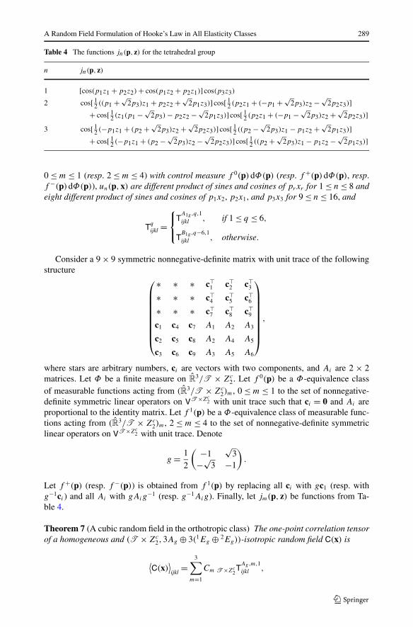
Table 4 The functions jn(p, z) for the tetrahedral group
n jn(p, z)
1 [cos(p1z1 + p2z2) + cos(p1z2 + p2z1)] cos(p3z3)
2 cos[ 12 ((p1 + √
2p3)z1 + p2z2 + √2p1z3)] cos[ 1
2 (p2z1 + (−p1 + √2p3)z2 − √
2p2z3)]+ cos[ 1
2 (z1(p1 − √2p3) − p2z2 − √
2p1z3)] cos[ 12 (p2z1 + (−p1 − √
2p3)z2 + √2p2z3)]
3 cos[ 12 (−p1z1 + (p2 + √
2p3)z2 + √2p2z3)] cos[ 1
2 ((p2 − √2p3)z1 − p1z2 + √
2p1z3)]+ cos[ 1
2 (−p1z1 + (p2 − √2p3)z2 − √
2p2z3)] cos[ 12 ((p2 + √
2p3)z1 − p1z2 − √2p1z3)]
0 ≤ m ≤ 1 (resp. 2 ≤ m ≤ 4) with control measure f 0(p)dΦ(p) (resp. f +(p)dΦ(p), resp.f −(p)dΦ(p)), un(p,x) are different product of sines and cosines of prxr for 1 ≤ n ≤ 8 andeight different product of sines and cosines of p1x2, p2x1, and p3x3 for 9 ≤ n ≤ 16, and
Tq
ijkl =⎧⎨
⎩
TA1g,q,1ijkl , if 1 ≤ q ≤ 6,
TB1g,q−6,1ijkl , otherwise.
Consider a 9 × 9 symmetric nonnegative-definite matrix with unit trace of the followingstructure
⎛
⎜⎜⎜⎜⎜⎜⎜⎜⎝
∗ ∗ ∗ c�1 c�
2 c�3
∗ ∗ ∗ c�4 c�
5 c�6
∗ ∗ ∗ c�7 c�
8 c�9
c1 c4 c7 A1 A2 A3
c2 c5 c8 A2 A4 A5
c3 c6 c9 A3 A5 A6
⎞
⎟⎟⎟⎟⎟⎟⎟⎟⎠
,
where stars are arbitrary numbers, ci are vectors with two components, and Ai are 2 × 2matrices. Let Φ be a finite measure on R
3/T × Zc2. Let f 0(p) be a Φ-equivalence class
of measurable functions acting from (R3/T × Zc2)m, 0 ≤ m ≤ 1 to the set of nonnegative-
definite symmetric linear operators on VT ×Zc2 with unit trace such that ci = 0 and Ai are
proportional to the identity matrix. Let f 1(p) be a Φ-equivalence class of measurable func-tions acting from (R3/T × Zc
2)m, 2 ≤ m ≤ 4 to the set of nonnegative-definite symmetriclinear operators on VT ×Zc
2 with unit trace. Denote
g = 1
2
( −1√
3−√
3 −1
).
Let f +(p) (resp. f −(p)) is obtained from f 1(p) by replacing all ci with gc1 (resp. withg−1ci ) and all Ai with gAig
−1 (resp. g−1Aig). Finally, let jm(p, z) be functions from Ta-ble 4.
Theorem 7 (A cubic random field in the orthotropic class) The one-point correlation tensorof a homogeneous and (T × Zc
2,3Ag ⊕ 3(1Eg ⊕ 2Eg))-isotropic random field C(x) is
⟨C(x)
⟩ijkl
=3∑
m=1
Cm T ×Zc2T
Ag,m,1ijkl ,
290 A. Malyarenko, M. Ostoja-Starzewski
where Cm ∈R. Its two-point correlation tensor has the form
⟨C(x),C(y)
⟩ = 1
6
1∑
m=0
∫
(R3/T ×Zc2)m
3∑
n=1
jn(p,y − x)f 0(p)dΦ(p)
+ 1
6
4∑
m=2
∫
(R3/T ×Zc2)m
[j1(p,y − x)f 1(p) + j2(p,y − x)f +(p)
+ j3(p,y − x)f −(p)]
dΦ(p).
The field has the form
C(x) =3∑
m=1
Cm T ×Zc2T
Ag,m,1ijkl + 1√
6
(9∑
q=1
24∑
n=1
1∑
m=0
∫
(R3/T ×Zc2)m
un(p,x)dZn0q (p)Tq
ijkl
+9∑
q=1
8∑
n=1
4∑
m=2
∫
(R3/T ×Zc2)m
un(p,x)dZn1q (p)Tq
ijkl
+9∑
q=1
16∑
n=9
4∑
m=2
∫
(R3/T ×Zc2)m
un(p,x)dZn+q (p)Tq
ijkl
+9∑
q=1
24∑
n=17
4∑
m=2
∫
(R3/T ×Zc2)m
un(p,x)dZn−q (p)Tq
ijkl
)
,
where un(p,x) are various products of sines and cosines of angles from Table 4,
Tq
ijkl =⎧⎨
⎩
T ×Zc2T
Ag,q,1ijkl , if 1 ≤ q ≤ 3
T ×Zc2TE2g,�q/2�−1,q mod 2+1
ijkl , otherwise,
and where (Zn01 (p), . . . ,Zn0
9 (p))� (resp. (Zn11 (p), . . . ,Zn1
9 (p))�, resp. (Zn+1 (p), . . . ,
Zn+9 (p))� resp. (Zn−
1 (p), . . . ,Zn−9 (p))�) are centred uncorrelated VT ×Zc
2 -valued randommeasures on (R3/T × Zc
2)m for 0 ≤ m ≤ 1 (resp. 2 ≤ m ≤ 4) with control measuref 0(p)dΦ(p) (resp. f 1(p)dΦ(p), resp. f +(p)dΦ(p), resp. f −(p)dΦ(p)).
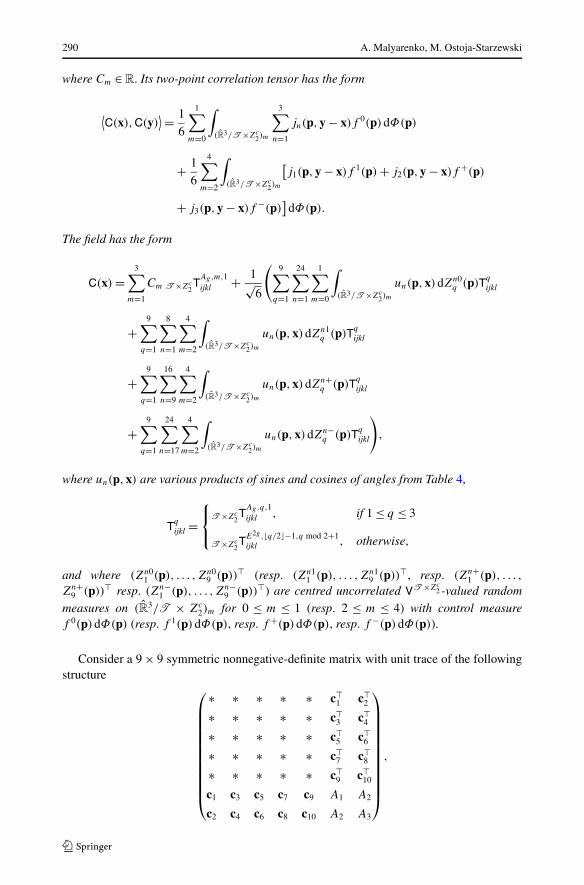
Consider a 9 × 9 symmetric nonnegative-definite matrix with unit trace of the followingstructure
⎛
⎜⎜⎜⎜⎜⎜⎜⎜⎜⎜⎜⎝
∗ ∗ ∗ ∗ ∗ c�1 c�
2
∗ ∗ ∗ ∗ ∗ c�3 c�
4
∗ ∗ ∗ ∗ ∗ c�5 c�
6
∗ ∗ ∗ ∗ ∗ c�7 c�
8
∗ ∗ ∗ ∗ ∗ c�9 c�
10
c1 c3 c5 c7 c9 A1 A2
c2 c4 c6 c8 c10 A2 A3
⎞
⎟⎟⎟⎟⎟⎟⎟⎟⎟⎟⎟⎠
,
A Random Field Formulation of Hooke’s Law in All Elasticity Classes 291
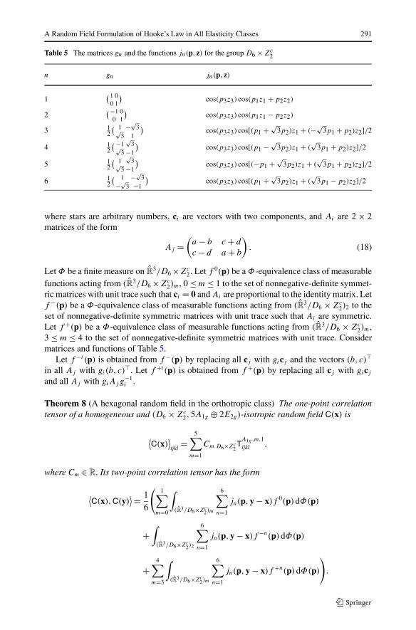
Table 5 The matrices gn and the functions jn(p, z) for the group D6 × Zc2
n gn jn(p, z)
1( 1 0
0 1
)cos(p3z3) cos(p1z1 + p2z2)
2(−1 0
0 1
)cos(p3z3) cos(p1z1 − p2z2)
3 12
( 1 −√3√
3 1
)cos(p3z3) cos[(p1 + √
3p2)z1 + (−√3p1 + p2)z2]/2
4 12
( −1√
3√3 −1
)cos(p3z3) cos[(p1 − √
3p2)z1 + (√
3p1 + p2)z2]/2
5 12
( 1√
3√3 −1
)cos(p3z3) cos[(−p1 + √
3p2)z1 + (√
3p1 + p2)z2]/2
6 12
( 1 −√3
−√3 −1
)cos(p3z3) cos[(p1 + √
3p2)z1 + (√
3p1 − p2)z2]/2
where stars are arbitrary numbers, ci are vectors with two components, and Ai are 2 × 2matrices of the form
Aj =(
a − b c + d
c − d a + b
). (18)
Let Φ be a finite measure on R3/D6 ×Zc
2. Let f 0(p) be a Φ-equivalence class of measurablefunctions acting from (R3/D6 ×Zc
2)m, 0 ≤ m ≤ 1 to the set of nonnegative-definite symmet-ric matrices with unit trace such that ci = 0 and Ai are proportional to the identity matrix. Letf −(p) be a Φ-equivalence class of measurable functions acting from (R3/D6 × Zc
2)2 to theset of nonnegative-definite symmetric matrices with unit trace such that Ai are symmetric.Let f +(p) be a Φ-equivalence class of measurable functions acting from (R3/D6 × Zc
2)m,3 ≤ m ≤ 4 to the set of nonnegative-definite symmetric matrices with unit trace. Considermatrices and functions of Table 5.
Let f −i (p) is obtained from f −(p) by replacing all cj with gicj and the vectors (b, c)�in all Aj with gi(b, c)�. Let f +i (p) is obtained from f +(p) by replacing all cj with gicj
and all Aj with giAjg−1i .
Theorem 8 (A hexagonal random field in the orthotropic class) The one-point correlationtensor of a homogeneous and (D6 × Zc
2,5A1g ⊕ 2E2g)-isotropic random field C(x) is
⟨C(x)
⟩ijkl
=5∑
m=1
Cm D6×Zc2T
A1g,m,1ijkl ,
where Cm ∈R. Its two-point correlation tensor has the form
⟨C(x),C(y)
⟩ = 1
6
(1∑
m=0
∫
(R3/D6×Zc2)m
6∑
n=1
jn(p,y − x)f 0(p)dΦ(p)
+∫
(R3/D6×Zc2)2
6∑
n=1
jn(p,y − x)f −n(p)dΦ(p)
+4∑
m=3
∫
(R3/D6×Zc2)m
6∑
n=1
jn(p,y − x)f +n(p)dΦ(p)
)
.
292 A. Malyarenko, M. Ostoja-Starzewski
The field has the form
C(x)ijkl =5∑
m=1
Cm D6×Zc2T
A1g,m,1ijkl + 1√
6
9∑
q=1
24∑
n=1
1∑
m=0
∫
(R3/D6×Zc2)m
un(p,x)dZ0nq (p)D6×Zc
2T
q
ijkl
+ 1√6
9∑
q=1
6∑
s=1
4s∑
n=4s−3
∫
(R3/D6×Zc2)2
un(p,x)dZ−nsq (p)D6×Zc
2T
q
ijkl
+ 1√6
9∑
q=1
6∑
s=1
4s∑
n=4s−3
4∑
m=3
∫
(R3/D6×Zc2)m
un(p,x)dZ+nsq (p)D6×Zc
2T
q
ijkl,
where (Z0n1 (p), . . . ,Z0n
9 (p))� (resp. (Z−ns1 (p), . . . ,Z−ns
9 (p))�, resp. (Z+ns1 (p), . . . ,
Z+ns9 (p))�) are centred uncorrelated VD6×Zc
2 -valued random measures on (R3/D6 × Zc2)m,
0 ≤ m ≤ 1 (resp. on (R3/D6 × Zc2)2, resp. on (R3/D6 × Zc
2)2, 3 ≤ m ≤ 4) with controlmeasure f 0(p)dΦ(p) (resp. f −s(p)dΦ(p), resp. f +s(p)dΦ(p)), un(p,x), 1 ≤ n ≤ 8 aredifferent product of sines and cosines of angles in Table 5, and where
Tq
ijkl =⎧⎨
⎩
D6×Zc2T
Ag,q,1ijkl , if 1 ≤ q ≤ 5
D6×Zc2TE2g,�q/2�−1,q mod 2+1
ijkl , otherwise.
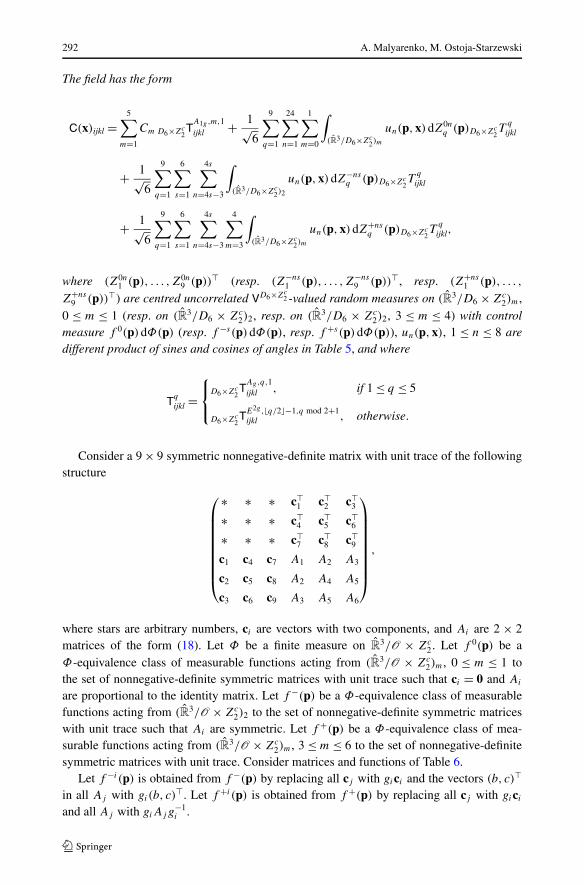
Consider a 9 × 9 symmetric nonnegative-definite matrix with unit trace of the followingstructure
⎛
⎜⎜⎜⎜⎜⎜⎜⎜⎝
∗ ∗ ∗ c�1 c�
2 c�3
∗ ∗ ∗ c�4 c�
5 c�6
∗ ∗ ∗ c�7 c�
8 c�9
c1 c4 c7 A1 A2 A3
c2 c5 c8 A2 A4 A5
c3 c6 c9 A3 A5 A6
⎞
⎟⎟⎟⎟⎟⎟⎟⎟⎠
,
where stars are arbitrary numbers, ci are vectors with two components, and Ai are 2 × 2matrices of the form (18). Let Φ be a finite measure on R
3/O × Zc2. Let f 0(p) be a
Φ-equivalence class of measurable functions acting from (R3/O × Zc2)m, 0 ≤ m ≤ 1 to
the set of nonnegative-definite symmetric matrices with unit trace such that ci = 0 and Ai
are proportional to the identity matrix. Let f −(p) be a Φ-equivalence class of measurablefunctions acting from (R3/O × Zc
2)2 to the set of nonnegative-definite symmetric matriceswith unit trace such that Ai are symmetric. Let f +(p) be a Φ-equivalence class of mea-surable functions acting from (R3/O × Zc
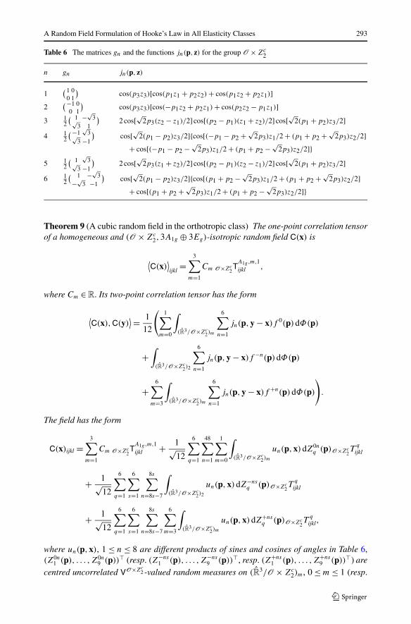
2)m, 3 ≤ m ≤ 6 to the set of nonnegative-definitesymmetric matrices with unit trace. Consider matrices and functions of Table 6.
Let f −i (p) is obtained from f −(p) by replacing all cj with gici and the vectors (b, c)�
in all Aj with gi(b, c)�. Let f +i (p) is obtained from f +(p) by replacing all cj with gici
and all Aj with giAjg−1i .
A Random Field Formulation of Hooke’s Law in All Elasticity Classes 293
Table 6 The matrices gn and the functions jn(p, z) for the group O × Zc2
n gn jn(p, z)
1( 1 0
0 1
)cos(p3z3)[cos(p1z1 + p2z2) + cos(p1z2 + p2z1)]
2(−1 0
0 1
)cos(p3z3)[cos(−p1z2 + p2z1) + cos(p2z2 − p1z1)]
3 12
( 1 −√3√
3 1
)2 cos[√2p3(z2 − z1)/2] cos[(p2 − p1)(z1 + z2)/2] cos[√2(p1 + p2)z3/2]
4 12
( −1√
3√3 −1
)cos[√2(p1 − p2)z3/2]{cos[(−p1 − p2 + √
2p3)z1/2 + (p1 + p2 + √2p3)z2/2]
+ cos[(−p1 − p2 − √2p3)z1/2 + (p1 + p2 − √
2p3)z2/2]}5 1
2
( 1√
3√3 −1
)2 cos[√2p3(z1 + z2)/2] cos[(p2 − p1)(z2 − z1)/2] cos[√2(p1 + p2)z3/2]
6 12
( 1 −√3
−√3 −1
)cos[√2(p1 − p2)z3/2]{cos[(p1 + p2 − √
2p3)z1/2 + (p1 + p2 + √2p3)z2/2]
+ cos[(p1 + p2 + √2p3)z1/2 + (p1 + p2 − √
2p3)z2/2]}
Theorem 9 (A cubic random field in the orthotropic class) The one-point correlation tensorof a homogeneous and (O × Zc
2,3A1g ⊕ 3Eg)-isotropic random field C(x) is
⟨C(x)
⟩ijkl
=3∑
m=1
Cm O×Zc2T
A1g,m,1ijkl ,
where Cm ∈R. Its two-point correlation tensor has the form
⟨C(x),C(y)
⟩ = 1
12
(1∑
m=0
∫
(R3/O×Zc2)m
6∑
n=1
jn(p,y − x)f 0(p)dΦ(p)
+∫
(R3/O×Zc2)2
6∑
n=1
jn(p,y − x)f −n(p)dΦ(p)
+6∑
m=3
∫
(R3/O×Zc2)m
6∑
n=1
jn(p,y − x)f +n(p)dΦ(p)
)
.
The field has the form
C(x)ijkl =3∑
m=1
Cm O×Zc2T
A1g,m,1ijkl + 1√
12
6∑
q=1
48∑
n=1
1∑
m=0
∫
(R3/O×Zc2)m
un(p,x)dZ0nq (p)O×Zc
2T
q
ijkl
+ 1√12
6∑
q=1
6∑
s=1
8s∑
n=8s−7
∫
(R3/O×Zc2)2
un(p,x)dZ−nsq (p)O×Zc
2T
q
ijkl
+ 1√12
6∑
q=1
6∑
s=1
8s∑
n=8s−7
6∑
m=3
∫
(R3/O×Zc2)m
un(p,x)dZ+nsq (p)O×Zc
2T
q
ijkl,
where un(p,x), 1 ≤ n ≤ 8 are different products of sines and cosines of angles in Table 6,(Z0n
1 (p), . . . ,Z0n9 (p))� (resp. (Z−ns
1 (p), . . . ,Z−ns9 (p))�, resp. (Z+ns
1 (p), . . . ,Z+ns9 (p))�) are
centred uncorrelated VO×Zc2 -valued random measures on (R3/O × Zc
2)m, 0 ≤ m ≤ 1 (resp.
294 A. Malyarenko, M. Ostoja-Starzewski
on (R3/O × Zc2)2, resp. on (R3/O × Zc
2)2, 3 ≤ m ≤ 6) with control measure f 0(p)dΦ(p)
(resp. f −s(p)dΦ(p), resp. f +s(p)dΦ(p)), and where
Tmijkl =
⎧⎨
⎩
O×Zc2T
Ag,m,1ijkl , if 1 ≤ m ≤ 3
O×Zc2TE2g,�m/2�−1,m mod 2+1
ijkl , if 4 ≤ m ≤ 9.
5.4 The Trigonal Class
Introduce the following notation:
j10(p, z) = cos(p1z1 + p3z3) cos(p2z2)
+ cos
[1
2(p1 + √
3p2)z1
]cos
[1
2(√
3p1 − p2)z2 + p3z3
]
+ cos
[1
2(p1 − √
3p2)z1
]cos
[1
2(−√
3p1 + p2)z2 + p3z3
].
Theorem 10 (A trigonal random field in the trigonal class) The one-point correlation tensorof a homogeneous and (D3 × Zc
2,6A1g)-isotropic random field C(x) is
⟨C(x)
⟩ijkl
=6∑
m=1
Cm D3×Zc2T
A1g,m,1ijkl ,
where Cm ∈R. Its two-point correlation tensor has the form
⟨C(x),C(y)
⟩ = 1
3
∫
R3/D3×Zc2
j10(p,y − x)f (p)dΦ(p),
where f (p) is the Φ-equivalence class of measurable functions acting from R3/D3 × Zc
2 tothe set of nonnegative-definite symmetric linear operators on VD3×Zc
2 with unit trace, and Φ
is a finite measure on R3/D3 × Zc
2. The field has the form
C(x)ijkl =6∑
m=1
Cm D3×Zc2T
A1g,m,1ijkl + 1√
3
6∑
m=1
12∑
n=1
∫
R3/D3×Zc2
un(p,x)dZmn(p)D3×Zc2T
A1g,m,1ijkl ,
where (Z1n(p), . . . ,Z6n(p))� are 12 centred uncorrelated VD3×Zc2 -valued random measures
on R3/D3 × Zc
2 with control measure f (p)dΦ(p), and where un(p,x), 1 ≤ n ≤ 4 are fourdifferent products of sines and cosines of p1x1 + p3x3 and p2x2, un(p,x), 5 ≤ n ≤ 8 arefour different product of sines and cosines of 1
2 (p1 +√3p2)x1 and 1
2 (√
3p1 −p2)x2 +p3x3,un(p,x), 9 ≤ n ≤ 12 are four different product of sines and cosines of 1
2 (p1 − √3p2)x1 and
12 (−√
3p1 + p2)x2 + p3x3.
A Random Field Formulation of Hooke’s Law in All Elasticity Classes 295
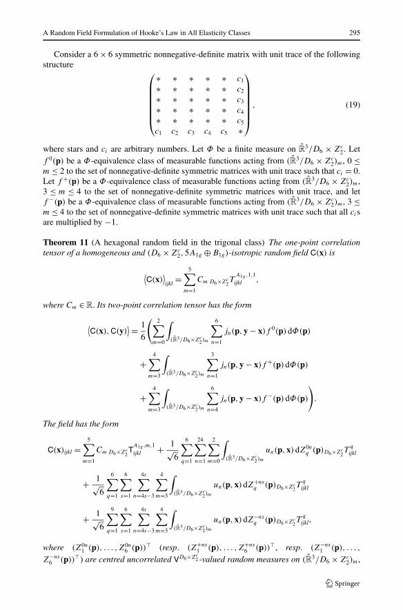
Consider a 6 × 6 symmetric nonnegative-definite matrix with unit trace of the followingstructure
⎛
⎜⎜⎜⎜⎜⎜⎝
∗ ∗ ∗ ∗ ∗ c1
∗ ∗ ∗ ∗ ∗ c2
∗ ∗ ∗ ∗ ∗ c3
∗ ∗ ∗ ∗ ∗ c4
∗ ∗ ∗ ∗ ∗ c5
c1 c2 c3 c4 c5 ∗
⎞
⎟⎟⎟⎟⎟⎟⎠
, (19)
where stars and ci are arbitrary numbers. Let Φ be a finite measure on R3/D6 × Zc
2. Letf 0(p) be a Φ-equivalence class of measurable functions acting from (R3/D6 × Zc
2)m, 0 ≤m ≤ 2 to the set of nonnegative-definite symmetric matrices with unit trace such that ci = 0.Let f +(p) be a Φ-equivalence class of measurable functions acting from (R3/D6 × Zc
2)m,3 ≤ m ≤ 4 to the set of nonnegative-definite symmetric matrices with unit trace, and letf −(p) be a Φ-equivalence class of measurable functions acting from (R3/D6 × Zc
2)m, 3 ≤m ≤ 4 to the set of nonnegative-definite symmetric matrices with unit trace such that all cisare multiplied by −1.
Theorem 11 (A hexagonal random field in the trigonal class) The one-point correlationtensor of a homogeneous and (D6 × Zc
2,5A1g ⊕ B1g)-isotropic random field C(x) is
⟨C(x)
⟩ijkl
=5∑
m=1
Cm D6×Zc2T
A1g,1,1ijkl ,
where Cm ∈R. Its two-point correlation tensor has the form
⟨C(x),C(y)
⟩ = 1
6
(2∑
m=0
∫
(R3/D6×Zc2)m
6∑
n=1
jn(p,y − x)f 0(p)dΦ(p)
+4∑
m=3
∫
(R3/D6×Zc2)m
3∑
n=1
jn(p,y − x)f +(p)dΦ(p)
+4∑
m=3
∫
(R3/D6×Zc2)m
6∑
n=4
jn(p,y − x)f −(p)dΦ(p)
)
.
The field has the form
C(x)ijkl =5∑
m=1
Cm D6×Zc2T
A1g,m,1ijkl + 1√
6
6∑
q=1
24∑
n=1
2∑
m=0
∫
(R3/D6×Zc2)m
un(p,x)dZ0nq (p)D6×Zc
2T
q
ijkl
+ 1√6
6∑
q=1
6∑
s=1
4s∑
n=4s−3
4∑
m=3
∫
(R3/D6×Zc2)m
un(p,x)dZ+nsq (p)D6×Zc
2T
q
ijkl
+ 1√6
9∑
q=1
6∑
s=1
4s∑
n=4s−3
4∑
m=3
∫
(R3/D6×Zc2)m
un(p,x)dZ−nsq (p)D6×Zc
2T
q
ijkl,
where (Z0n1 (p), . . . ,Z0n
6 (p))� (resp. (Z+ns1 (p), . . . ,Z+ns
6 (p))�, resp. (Z−ns1 (p), . . . ,
Z−ns6 (p))�) are centred uncorrelated VD6×Zc
2 -valued random measures on (R3/D6 × Zc2)m,
296 A. Malyarenko, M. Ostoja-Starzewski
0 ≤ m ≤ 2 (resp. on (R3/D6 × Zc2)m, 3 ≤ m ≤ 4) with control measure f 0(p)dΦ(p) (resp.
f +(p)dΦ(p), resp. f −(p)dΦ(p)), un(p,x), 1 ≤ n ≤ 8 are different product of sines andcosines of angles in Table 5, and where
Tq
ijkl =⎧⎨
⎩D6×Zc
2T
A1g,q,1ijkl , if 1 ≤ q ≤ 5,
D6×Zc2T
B1g,m,1ijkl , otherwise.
5.5 The Tetragonal Class
Theorem 12 (A tetragonal random field in the tetragonal class) The one-point correlationtensor of a homogeneous and (D4 × Zc
2,6A1g)-isotropic random field C(x) is
⟨C(x)
⟩ijkl
=6∑
m=1
Cm D4×Zc2T
A1g,m,1ijkl ,
where Cm ∈R. Its two-point correlation tensor has the form
⟨C(x),C(y)
⟩ = 1
2
∫
R3/D4×Zc2
[cos
(p1(x1 − y1)
)cosm
(p2(x2 − y2)
)
+ cos(p1(x2 − y2)
)cos
(p2(x1 − y1)
)]cos
(p3(x3 − y3)
)f (p)dΦ(p),
where f (p) is a Φ-equivalence class of measurable functions acting from R3/D4 × Zc
2 tothe set of nonnegative-definite symmetric linear operators on VD4×Zc
2 with unit trace, and Φ
is a finite measure on R3/D4 × Zc
2. The field has the form
C(x)ijkl =6∑
m=1
Cm D4×Zc2T
A1g,m,1ijkl + 1√
2
6∑
m=1
16∑
n=1
∫
R3/D4×Zc2
un(p,x)dZmn(p)D4×Zc2T
A1g,m,1ijkl ,
where (Z1n(p), . . . ,Z6n(p))� are 16 centred uncorrelated VD4×Zc2 -valued random measures
on R3/D4 × Zc
2 with control measure f (p)dΦ(p), and where un(p,x) are eight differentproduct of sines and cosines of prxr for 1 ≤ n ≤ 8 and eight different product of sines andcosines of p1x2, p2x1, and p3x3 for 9 ≤ n ≤ 16.
Consider a 6 × 6 symmetric nonnegative-definite matrix with unit trace of the structure(19). Let Φ be a finite measure on R
3/D8 ×Zc2. Let f 0(p) be a Φ-equivalence class of mea-
surable functions acting from (R3/D8 × Zc2)m, 0 ≤ m ≤ 1 to the set of nonnegative-definite
symmetric matrices with unit trace such that ci = 0. Let f +(p) be a Φ-equivalence classof measurable functions acting from (R3/D8 × Zc
2)m, 2 ≤ m ≤ 4 to the set of nonnegative-definite symmetric matrices with unit trace, and let f −(p) be a Φ-equivalence class of mea-surable functions acting from (R3/D8 × Zc
2)m, 2 ≤ m ≤ 4 to the set of nonnegative-definitesymmetric matrices with unit trace such that all cis are multiplied by −1.
A Random Field Formulation of Hooke’s Law in All Elasticity Classes 297
Introduce the following notation.
j+13(p, z) = 2 cos(p3z3)
[cos(p1z1 + p2z2) + cos(p2z1 − p1z2)
+ cos((p1 + p2)(z1 + z2)/
√2)
+ cos((p2z2 − p1z1)/
√2 − p3z3
)cos
((p1z2 + p2z1)/
√2)]
,
j−13(p, z) = cos(p3z3)
[2 cos(p1z1 − p2z2) + 2 cos(p2z1 + p1z2)
+ cos((p1z1 + p2z2)/
√2)
cos((p2z1 − p1z2)/
√2)]
.
Theorem 13 (An octagonal random field in the tetragonal class) The one-point correlationtensor of a homogeneous and (D8 × Zc
2,5A1g ⊕ B1g)-isotropic random field C(x) is
⟨C(x)
⟩ijkl
=5∑
m=1
Cm D8×Zc2T
A1g,1,1ijkl ,
where Cm ∈R. Its two-point correlation tensor has the form
⟨C(x),C(y)
⟩ = 1
4
(1∑
m=0
∫
(R3/D8×Zc2)m
(j+
13(p,y − x) + j−13(p,y − x)
)f 0(p)dΦ(p)
+4∑
m=2
∫
(R3/D8×Zc2)m
j+13(p,y − x)f +(p)dΦ(p)
+4∑
m=2
∫
(R3/D8×Zc2)m
j−13(p,y − x)f −(p)dΦ(p)
)
.
The field has the form
C(x)ijkl =5∑
m=1
Cm D8×Zc2T
A1g,m,1ijkl + 1
2
6∑
q=1
32∑
n=1
1∑
m=0
∫
(R3/D8×Zc2)m
un(p,x)dZ0nq (p)D8×Zc
2T
q
ijkl
+ 1
2
6∑
q=1
16∑
n=1
4∑
m=2
∫
(R3/D8×Zc2)m
un(p,x)dZ+nq (p)D8×Zc
2T
q
ijkl
+ 1
2
6∑
q=1
32∑
n=17
4∑
m=2
∫
(R3/D8×Zc2)m
un(p,x)dZ−nq (p)D8×Zc
2T
q
ijkl,
where (Z0n1 (p), . . . ,Z0n
6 (p))� (resp. (Z+n1 (p), . . . ,Z+n
6 (p))�, resp. (Z−n1 (p), . . . ,Z−n
6 (p))�)are centred uncorrelated VD8×Zc
2 -valued random measures on (R3/D8 × Zc2)m, 0 ≤
m ≤ 1 (resp. on (R3/D8 × Zc2)m, 2 ≤ m ≤ 4) with control measure f 0(p)dΦ(p) (resp.
f +(p)dΦ(p), resp. f −(p)dΦ(p)), un(p,x), 1 ≤ n ≤ 8 are different product of sines andcosines of angles in Table 5, and where
Tq
ijkl =⎧⎨
⎩D8×Zc
2T
A1g,q,1ijkl , if 1 ≤ q ≤ 5,
D8×Zc2T
B1g,m,1ijkl , otherwise.
298 A. Malyarenko, M. Ostoja-Starzewski
5.6 The Transverse Isotropic Class
Theorem 14 (A transverse isotropic random field in the transverse isotropic class) The one-point correlation tensor of the homogeneous and (O(2)×Zc
2,5U 0gg)-isotropic mean-squarecontinuous random field C(x) has the form
⟨C(x)
⟩ =5∑
m=1
Cm O(2)×Zc2T
U0gg,m,1ijkl ,
where Cm ∈R. Its two-point correlation tensor has the form
⟨C(x),C(y)
⟩ =∫
R3/O(2)×Zc2
J0
(√(p2
1 + p22
)((y1 − x1)2 + (y2 − x2)2
))
× cos(p3(y3 − x3)
)f (p)dΦ(p),
where Φ is a measure on R3/O(2) × Zc
2, and f (p) is a Φ-equivalence class of measurablefunctions on R
3/O(2) × Zc2 with values in the compact set of all nonnegative-definite linear
operators in the space VO(2)×Zc2 with unit trace. The field has the form
C(x) =5∑
m=1
Cm O(2)×Zc2T
0⊗A,m,1ijkl
+5∑
m=1
∫
R3/O(2)×Zc2
J0
(√(p2
1 + p22
)(x2
1 + x22
))
× (cos(p3x3)dZ01m(p)O(2)×Zc
2T
U0gg,m,1ijkl + sin(p3x3)dZ02m(p)O(2)×Zc
2T
U0gg,m,1ijkl
)
+ √2
∞∑
=1
5∑
m=1
∫
R3/O(2)×Zc2
J
(√(p2
1 + p22
)(x2
1 + x22
))
× (cos(p3x3) cos( ϕp)dZ 1m(p)O(2)×Zc
2T
U0gg,m,1ijkl
+ cos(p3x3) sin( ϕp)dZ 2m(p)O(2)×Zc2T
U0gg,m,1ijkl
+ sin(p3x3) cos( ϕp)dZ 3m(p)O(2)×Zc2T
U0gg,m,1ijkl
+ sin(p3x3) sin( ϕp)dZ 4m(p)O(2)×Zc2T
U0gg,m,1ijkl
),
where (Z i1(p), . . . ,Z i5(p))� are centred uncorrelated VO(2)×Zc2 -valued random measures
on R3/O(2) × Zc
2 with control measure f (p)dΦ(p).
5.7 The Cubic Class
Theorem 15 (A cubic random field in the cubic class) The one-point correlation tensor ofthe homogeneous and (O × Zc
2,3A1g)-isotropic mean-square continuous random field C(x)
has the form
⟨C(x)
⟩ =3∑
m=1
Cm O×Zc2T
A1g,m,1ijkl ,
A Random Field Formulation of Hooke’s Law in All Elasticity Classes 299
where Cm ∈R. Its two-point correlation tensor has the form
⟨C(x),C(y)
⟩ =∫
R3/O×Zc2
8∑
m=0
jm(x − y,p)f (p)dΦ(p),
where the functions jm(z,p) are shown in Table 6, Φ is a measure on R3/O ×Zc
2, and f (p)
is a Φ-equivalence class of measurable functions on R3/O × Zc
2 with values in the compactset of all nonnegative-definite linear operators in the space VO×Zc
2 with unit trace. The fieldhas the form
C(x) =3∑
m=1
Cm O×Zc2T
A1g,m,1ijkl +
3∑
m=1
48∑
n=1
∫
R3/O×Zc2
un(x,p)dZmn(p)O×Zc2T
A1g,m,1ijkl ,
where (Z1n(p), . . . ,Z3n(p))� are 48 centred uncorrelated VO×Zc2 -valued random measures
on R3/O × Zc
2 with control measure f (p)dμ(p), and where un(x,p) are different productsof sines and cosines of angles from Table 6.
5.8 The Isotropic Class
Theorem 16 (An isotropic random field in the isotropic class) The one-point correlationtensor of the homogeneous and (O(3),2U 0g)-isotropic mean-square continuous randomfield C(x) has the form
⟨C(x)
⟩ = C1δij δkl + C2(δikδjl + δilδjk), Cm ∈R.
Its two-point correlation tensor has the form
⟨C(x),C(y)
⟩ =∫ ∞
0
sin(λ‖y − x‖)λ‖y − x‖ f (λ)dΦ(λ),
where Φ(λ) is a finite measure on [0,∞),
f (λ) =(
v1(λ) v2(λ)
v2(λ) 1 − v1(λ)
),
and where v(λ) = (v1(λ), v2(λ))� is a Φ-equivalence class of measurable functions on[0,∞) taking values in the closed disk (v1(λ)− 1/2)2 + v2
2(λ) ≤ 1/4. The field itself has theform
Cijkl(ρ, θ,ϕ) = C1δij δkl + C2(δikδjl + δilδjk) + 2√
π
∞∑
=0
∑
m=
Sm (θ,ϕ)
∫ ∞
0j (λρ)
× (O(3)T
0,1,0ijkl dZm
1(λ) + O(3)T0,2,0ijkl dZm
2(λ)),
where (Zm 1,Z
m 2)
� is the set of mutually uncorrelated VO(3)-valued random measures withf (λ)dΦ(λ) as their common control measure.
300 A. Malyarenko, M. Ostoja-Starzewski
6 Conclusions
Hooke’s law describes the physical phenomenon of elasticity and belongs to the family oflinear constitutive laws, see [25]. In general, a linear constitutive law is an element of asubspace of the tensor product V ⊗(p+q), where p (resp. q) is the rank of tensors in the first(resp. second) state tensor space. Denote by U the restriction of the representation g →g⊗(p+q) to the above subspace. Consider U as a group action. The orbit types of this actionare called the classes of the phenomenon under consideration (e.g., photoelasticity classes,piezoelectricity classes and so on). All symmetry classes of all possible linear constitutivelaws were described in [25, 26].
For each class, one can consider its fixed point set VH ⊂ V ⊗(p+q), a group K withH ⊆ K ⊆ N(H), and the restriction U of the representation g → g⊗(p+q) of the groupK to VH . Calculating the general form of the one-point and two-point correlation tensors ofthe corresponding homogeneous and (K,U)-isotropic random field and the spectral expan-sion of the field in terms of stochastic integrals with respect to orthogonal scattered randommeasures is an interesting research question.
There are two principal uses of the results obtained here. The first one is to model andsimulate any statistically wide-sense homogeneous and isotropic, linear hyperelastic, ran-dom medium. One example is a polycrystal made of grains belonging to a specific crystalclass, while another example is a mesoscale continuum defined through upscaling of a ran-dom material on scales smaller than the RVE; if the upscaling is conducted on the RVElevel, there is no spatial randomness and the continuum model is deterministic. Here onewould proceed in the following steps:
– for a given microstructure, determine the one- and two-point statistics using some exper-imental and/or image-based computational methods;
– calibrate the entire correlation structure of the elasticity TRF;– simulate the realisations of this TRF.
The second application of our results is their use as input of a random mesoscale contin-uum (Fig. 1(c)) into stochastic field equations such as SPDEs and SFEs.
Acknowledgements We are grateful to the two anonymous referees for their remarks that helped to im-prove the paper significantly.
Open Access This article is distributed under the terms of the Creative Commons Attribution 4.0 Inter-national License (http://creativecommons.org/licenses/by/4.0/), which permits unrestricted use, distribution,and reproduction in any medium, provided you give appropriate credit to the original author(s) and the source,provide a link to the Creative Commons license, and indicate if changes were made.
References
1. Altmann, S.L., Herzig, P.: Point-Group Theory Tables. Oxford Science Publications Clarendon, Oxford(1994)
2. Auffray, N., Kolev, B., Petitot, M.: On anisotropic polynomial relations for the elasticity tensor. J. Elast.115(1), 77–103 (2014)
3. Bourbaki, N.: Integration. II. Chapters 7–9. In: Elements of Mathematics (Berlin). Springer, Berlin(2004)
4. Brock, C. (ed.): International Tables for Crystallography, vol. A–G, 4th edn. Wiley, New York (2014)5. Cramér, H.: On the theory of stationary random processes. Ann. Math. (2) 41, 215–230 (1940)6. Duistermaat, J.J., Kolk, J.A.C.: Lie Groups. Universitext. Springer, Berlin (2000)7. Forte, S., Vianello, M.: Symmetry classes for elasticity tensors. J. Elast. 43(2), 81–108 (1996)
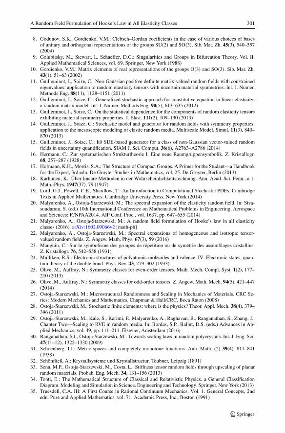
A Random Field Formulation of Hooke’s Law in All Elasticity Classes 301
8. Godunov, S.K., Gordienko, V.M.: Clebsch–Gordan coefficients in the case of various choices of basesof unitary and orthogonal representations of the groups SU(2) and SO(3). Sib. Mat. Zh. 45(3), 540–557(2004)
9. Golubitsky, M., Stewart, I., Schaeffer, D.G.: Singularities and Groups in Bifurcation Theory. Vol. II.Applied Mathematical Sciences, vol. 69. Springer, New York (1988)
10. Gordienko, V.M.: Matrix elements of real representations of the groups O(3) and SO(3). Sib. Mat. Zh.43(1), 51–63 (2002)
11. Guilleminot, J., Soize, C.: Non-Gaussian positive-definite matrix-valued random fields with constrainedeigenvalues: application to random elasticity tensors with uncertain material symmetries. Int. J. Numer.Methods Eng. 88(11), 1128–1151 (2011)
12. Guilleminot, J., Soize, C.: Generalized stochastic approach for constitutive equation in linear elasticity:a random matrix model. Int. J. Numer. Methods Eng. 90(5), 613–635 (2012)
13. Guilleminot, J., Soize, C.: On the statistical dependence for the components of random elasticity tensorsexhibiting material symmetry properties. J. Elast. 111(2), 109–130 (2013)
14. Guilleminot, J., Soize, C.: Stochastic model and generator for random fields with symmetry properties:application to the mesoscopic modeling of elastic random media. Multiscale Model. Simul. 11(3), 840–870 (2013)
15. Guilleminot, J., Soize, C.: Itô SDE-based generator for a class of non-Gaussian vector-valued randomfields in uncertainty quantification. SIAM J. Sci. Comput. 36(6), A2763–A2786 (2014)
16. Hermann, C.: Zur systematischen Strukturtheorie I. Eine neue Raumgruppensymbolik. Z. Kristallogr.68, 257–287 (1928)
17. Hofmann, K.H., Morris, S.A.: The Structure of Compact Groups. A Primer for the Student—a Handbookfor the Expert, 3rd edn. De Gruyter Studies in Mathematics, vol. 25. De Gruyter, Berlin (2013)
18. Karhunen, K.: Über lineare Methoden in der Wahrscheinlichkeitsrechnung. Ann. Acad. Sci. Fenn., a 1.Math.-Phys. 1947(37), 79 (1947)
19. Lord, G.J., Powell, C.E., Shardlow, T.: An Introduction to Computational Stochastic PDEs. CambridgeTexts in Applied Mathematics. Cambridge University Press, New York (2014)
20. Malyarenko, A., Ostoja-Starzewski, M.: The spectral expansion of the elasticity random field. In: Siva-sundaram, S. (ed.) 10th International Conference on Mathematical Problems in Engineering, Aerospaceand Sciences: ICNPAA2014. AIP Conf. Proc., vol. 1637, pp. 647–655 (2014)
21. Malyarenko, A., Ostoja-Starzewski, M.: A random field formulation of Hooke’s law in all elasticityclasses (2016). arXiv:1602.09066v2 [math-ph]
22. Malyarenko, A., Ostoja-Starzewski, M.: Spectral expansions of homogeneous and isotropic tensor-valued random fields. Z. Angew. Math. Phys. 67(3), 59 (2016)
23. Mauguin, C.: Sur le symbolisme des groupes de répetition ou de symétrie des assemblages cristallins.Z. Kristallogr. 76, 542–558 (1931)
24. Mulliken, R.S.: Electronic structures of polyatomic molecules and valence. IV. Electronic states, quan-tum theory of the double bond. Phys. Rev. 43, 279–302 (1933)
25. Olive, M., Auffray, N.: Symmetry classes for even-order tensors. Math. Mech. Compl. Syst. 1(2), 177–210 (2013)
26. Olive, M., Auffray, N.: Symmetry classes for odd-order tensors. Z. Angew. Math. Mech. 94(5), 421–447(2014)
27. Ostoja-Starzewski, M.: Microstructural Randomness and Scaling in Mechanics of Materials. CRC Se-ries: Modern Mechanics and Mathematics. Chapman & Hall/CRC, Boca Raton (2008)
28. Ostoja-Starzewski, M.: Stochastic finite elements: where is the physics? Theor. Appl. Mech. 38(4), 379–396 (2011)
29. Ostoja-Starzewski, M., Kale, S., Karimi, P., Malyarenko, A., Raghavan, B., Ranganathan, S., Zhang, J.:Chapter Two—Scaling to RVE in random media. In: Bordas, S.P., Balint, D.S. (eds.) Advances in Ap-plied Mechanics, vol. 49, pp. 111–211. Elsevier, Amsterdam (2016)
30. Ranganathan, S.I., Ostoja-Starzewski, M.: Towards scaling laws in random polycrystals. Int. J. Eng. Sci.47(11–12), 1322–1330 (2009)
31. Schoenberg, I.J.: Metric spaces and completely monotone functions. Ann. Math. (2) 39(4), 811–841(1938)
32. Schönfließ, A.: Krystallsysteme und Krystallstructur. Teubner, Leipzig (1891)33. Sena, M.P., Ostoja-Starzewski, M., Costa, L.: Stiffness tensor random fields through upscaling of planar
random materials. Probab. Eng. Mech. 34, 131–156 (2013)34. Tonti, E.: The Mathematical Structure of Classical and Relativistic Physics. a General Classification
Diagram. Modeling and Simulation in Science. Engineering and Technology. Springer, New York (2013)35. Truesdell, C.A. III: A First Course in Rational Continuum Mechanics. Vol. 1. General Concepts, 2nd
edn. Pure and Applied Mathematics, vol. 71. Academic Press, Inc., Boston (1991)

302 A. Malyarenko, M. Ostoja-Starzewski
36. Yaglom, A.M.: Homogeneous and isotropic turbulence in a viscous compressible fluid. Izv. Akad. NaukSSSR, Ser. Geogr. Geofiz. 12, 501–522 (1948)
37. Yaglom, A.M.: Second-order homogeneous random fields. In: Proc. 4th Berkeley Sympos. Math. Statist.and Prob., vol. II, pp. 593–622. Univ. California Press, Berkeley (1961)