Embed Size (px)
Citation preview

1
A Random Access Protocol for Pilot Allocationin Crowded Massive MIMO Systems
Emil Bjornson, Member, IEEE, Elisabeth de Carvalho, Senior Member, IEEE,Jesper H. Sørensen, Member, IEEE, Erik G. Larsson, Fellow, IEEE, Petar Popovski, Fellow, IEEE
Abstract—The Massive MIMO (multiple-input multiple-output) technology has great potential to manage the rapidgrowth of wireless data traffic. Massive MIMO achievestremendous spectral efficiency by spatial multiplexing ofmany tens of user equipments (UEs). These gains areonly achieved in practice if many more UEs can connectefficiently to the network than today. As the number ofUEs increases, while each UE intermittently accesses thenetwork, the random access functionality becomes essentialto share the limited number of pilots among the UEs. In thispaper, we revisit the random access problem in the MassiveMIMO context and develop a reengineered protocol, termedstrongest-user collision resolution (SUCRe). An accessing UEasks for a dedicated pilot by sending an uncoordinatedrandom access pilot, with a risk that other UEs send the samepilot. The favorable propagation of Massive MIMO channelsis utilized to enable distributed collision detection at each UE,thereby determining the strength of the contenders’ signalsand deciding to repeat the pilot if the UE judges that itssignal at the receiver is the strongest. The SUCRe protocolresolves the vast majority of all pilot collisions in crowdedurban scenarios and continues to admit UEs efficiently inoverloaded networks.
Index Terms—Massive MIMO, random access, collisionresolution.
I. INTRODUCTION
The number of wirelessly connected devices and theirrespective data traffic are growing rapidly as we transi-tion into the fully networked society [1]. The growth iscurrently driven by video streaming, social networking,
c© 2017 IEEE. Personal use of this material is permitted. Permissionfrom IEEE must be obtained for all other uses, in any current or futuremedia, including reprinting/republishing this material for advertisingor promotional purposes, creating new collective works, for resale orredistribution to servers or lists, or reuse of any copyrighted componentof this work in other works.
E. Bjornson and E. G. Larsson are with the Department of ElectricalEngineering (ISY), Linkoping University, Linkoping, Sweden (email:[email protected], [email protected]).
E. de Carvalho, J. H. Sørensen, and P. Popovski are with the De-partment of Electronic Systems, Aalborg University, Aalborg, Denmark(email: [email protected], [email protected]).
This work was presented in part at the IEEE International Conferenceon Communications (ICC), Kuala Lumpur, Malaysia, May 2016.
This work was performed partly in the framework of the Danish Coun-cil for Independent Research (DFF133500273), the Horizon 2020 projectFANTASTIC-5G (ICT-671660), the EU FP7 project MAMMOET (ICT-619086), ELLIIT, and CENIIT. The authors would like to acknowledgethe contributions of the colleagues in FANTASTIC-5G and MAMMOET.
Digital Object Identifier 10.1109/TWC.2017.2660489
and new use cases, such as machine-to-machine commu-nication and internet of things. In dense urban scenarios,the METIS project predicts a future with up to 200.000devices per km2 and an associated data volume of 500Gbyte/month/device [2]. These are massive numbers thatcall for radical changes in the network infrastructureto avoid congestion and guarantee service quality andavailability. A fair amount of the traffic is expected tobe offloaded to WiFi and small-cell-technology operatingat mm-wave frequencies, but macro cellular networksoperating at frequencies of one or a few GHz will remainto define the coverage, mobility support, and guaranteedservice quality. Hence, future cellular networks need tohandle urban deployment with massive numbers of con-nected UEs that request massive data volumes [3].
Since the cellular frequency bands are scarce, orders-of-magnitude capacity improvements are only possible byradically increasing the spectral efficiency (SE) [bit/s/Hz].The Massive MIMO network topology, proposed in theseminal paper [4], can theoretically deliver such extraor-dinary improvements [5]. The gains are achieved by spatialmultiplexing, where base stations (BSs) with hundreds ofantennas are utilized to serve tens of UEs per cell, at thesame time-frequency resource. Massive MIMO is primar-ily a technology for time-division duplexing (TDD) [6],where scalable channel estimation protocols are achievedby only requiring uplink pilots and utilizing channelreciprocity to obtain downlink channel estimates [7]. Thecommunication-theoretic performance and asymptotic lim-its of Massive MIMO have been analyzed extensivelyin recent years; see for instance [4]–[6], [8]–[15]. Theseworks have focused on the performance achieved by activeUEs, mainly in homogeneously loaded cells, while thenetwork access functionality has received little attention[16]. It is important to note that the building block ofthe traffic is data packets, which are generated in anintermittent and unpredictable fashion in all non-streamingapplications. For example, web browsing and social net-work applications are characterized by bursty on-off trafficwhere intensive download activities are interwoven withlong periods of silence. Many UEs thus switch betweenbeing active and inactive at a frequent and irregular basis.Since Massive MIMO will be deployed to handle, say, 10×higher UE densities than in current systems, the number
arX
iv:1
604.
0424
8v2
[cs
.IT
] 1
1 Fe
b 20
17

2
1. Random Preamble
2. Random Access Response
3. RRC Connection Request
4. Centralized Contention Resolution
UE BS
Fig. 1: The PRACH protocol of the LTE system.
of UEs that switch between active and inactive mode in agiven time interval will be 10× higher as well. Scalableand efficient access protocols are thus mandatory.
A. Random Access Functionality in LTE
Before we propose a new highly scalable access proto-col, we describe the conventional protocol used on thePhysical Random Access Channel (PRACH) of Long-Term Evolution (LTE). It consists of four steps [17], asillustrated in Fig. 1. In Step 1, each accessing UE picks apreamble at random from a predefined set. The preambleis an entity that enables synchronization towards the BS.It does not carry specific reservation information or dataand thus can be viewed as a pilot sequence. Since UEsthat wish to access the network are not coordinated inpicking the preambles, a collision occurs if two or moreUEs select the same preamble simultaneously. A BS inLTE only detects if a specific preamble is active or not inStep 1 [18]. In Step 2, the BS sends a random accessresponse corresponding to each activated preamble, toconvey physical parameters (e.g., timing advance) andallocate a resource to the UE (or UEs) that activated thepreamble. In Step 3, each UE that has received a responseto its preamble transmission sends a RRC (Radio ResourceControl) Connection Request in order to request resourcesfor subsequent data transmission. If more than one UEactivated the preamble, then all these UEs use the sameresource to send their RRC connection request in Step 3and this collision is detected by the BS. Step 4 is calledcontention resolution and contains one or multiple stepsto resolve the collision. This is a complicated procedurethat might result in that all colliding UEs need to make anew access attempt after a random waiting time.
B. Prior Work on Random Access in Massive MIMO
Conventional cellular networks allocate dedicated re-sources to each active UE, thus the BS needs to convey thetime-frequency positions of these resources. In contrast,Massive MIMO systems allocate all time-frequency re-sources to all active UEs, and separate them spatially basedon their pilot sequences. The number of pilots is limited
by the size of the channel coherence block. In the originalMassive MIMO concept of [4] the UEs within a cell usemutually orthogonal pilots, while the necessary reuse ofpilots across cells causes inter-cell pilot contamination thatleads to additional interference [8].
In crowded urban scenarios, the total number of activeand inactive UEs residing in a cell is also much larger thanthe number of available pilot sequences. Hence, a pilotcannot be permanently associated with a UE in the cellbut need to be opportunistically allocated and deallocatedto follow its unpredictable intermittent data traffic pattern.Random access (RA) mechanisms can be used for suchpilot allocation, but must be designed to resolve collisionsin crowded cells without excessive access delays. The pa-pers [19]–[21] propose protocols where UEs can transmitdata whenever they like by selecting pilots at random froma common pool. This eliminates access delays, at the costof pilot collisions that cause intra-cell pilot contamination.The collisions are expressed as a graph code in [19] andbelief propagation is used to mitigate pilot contamination,by utilizing the principles of coded random access [22],[23]. Several SE expressions are derived in [20] andutilized to optimize the UE activation probability and pilotlength. Asynchronous UE timings are utilized in [21] todetect and resolve pilot collisions in RA.
In this paper, we explore the alternative solution thateach UE needs to be assigned a pilot sequence beforetransmitting payload data, to avoid intra-cell pilot col-lisions and actualize the payload transmission situationconsidered in the main body of Massive MIMO research[4]–[6], [8]–[11]. We focus on urban deployments withsmall initial timing variations and propose a new RAprotocol for UEs that wish to access the network. Theprotocol can resolve RA collisions in a distributed andscalable way, by exploiting special properties of MassiveMIMO channels. A preliminary version of the protocolwas described in [24].
C. Outline and Notation
The remainder of this paper is organized as follows.Section II describes the proposed RA protocol assumingarbitrary Massive MIMO channels, while Section III an-alyzes the performance with uncorrelated Rayleigh fad-ing channels. Section IV provides numerical results thatshow how the proposed protocol can resolve severe RAcollisions and operate under very high load. The mainconclusions are summarized in Section V.
The following notation is used throughout the paper.The transpose, conjugate-transpose, and conjugate of amatrix X are denoted by XT, XH, and X∗, respectively.We let IM denote the M ×M identity matrix, whereas‖ · ‖ and | · | stand for the Euclidean norm of a vector andcardinality of a set, respectively. The notations E{·} andV{·} indicate the expectation and variance with respect toa random variable. We use N (·, ·) to denote a Gaussian

3
distribution, CN (·, ·) to denote a circularly-symmetriccomplex Gaussian distribution, B(·, ·) to denote a binomialdistribution, and χn to denote a chi-distribution with ndegrees of freedom. We use C and R to denote spacesof complex-valued and real-valued numbers, respectively.The Gamma function is denoted by Γ(·).
II. PROPOSED RANDOM ACCESS PROTOCOL
We consider cellular networks where each BS isequipped with M antennas. The system operates in TDDmode and the time-frequency resources are divided intocoherence blocks of T channel uses, dimensioned suchthat the channel responses between each BS and its UEsare constant and frequency flat within a block, whilethey vary between blocks. This can be implemented usingorthogonal frequency-division multiplexing (OFDM). Welet Ui denote the set of UEs that reside in cell i. Atany given time, only a subset Ai ⊂ Ui of the UEsare active in the sense that they are transmitting and/orreceiving data. Note that in the scenarios relevant forMassive MIMO deployment, we typically have a verylarge UE set: |Ui| � T . However, the active UEs satisfy|Ai| < T , thus the BS can temporarily assign orthogonalpilot sequences to these UEs and reclaim them when theirrespective transmissions are finished.
The coherence blocks are divided into two categories:payload data blocks and random access blocks. For eachcell i, the first category is used for uplink (UL) anddownlink (DL) data transmission to the UEs in the set Ai.These UEs have temporarily been allocated |Ai| mutuallyorthogonal pilot sequences, which however are reused inother cells (using some reuse factor that guarantees lowpilot contamination [5]). The payload data blocks can beoperated as in the classical Massive MIMO works [4]–[6], [8]–[11], which provide methods to achieve high datarates.
The second category is dedicated for RA from inactiveUEs (i.e., some of those in Ui \ Ai) that wish to beadmitted to the payload data blocks; that is, to be allocateda temporary dedicated pilot. This category has not beenstudied in the Massive MIMO context and is the mainfocus of this paper. The time-frequency location of theRA blocks is different between adjacent cells, as illustratedin Fig. 2. This design choice protects the RA procedurefrom the strongest forms of inter-cell interference, as willbe shown later.
A. Strongest-user collision resolution (SUCRe)—Overview
The key contribution of this paper is the strongest-user collision resolution (SUCRe) protocol, which is anefficient way to operate the RA blocks in beyond-LTEMassive MIMO systems. We first give a brief overview ofthe protocol and then provide the exact analytical details.The four main steps of the SUCRe protocol are illustratedin Fig. 3. There is also a preliminary Step 0 in which the
BS broadcasts a control signal. Each UE uses this signal toestimate its average channel gain and to synchronize itselftowards the BS. In OFDM, the UE and the BS need tobe synchronized in frequency and the timing delay can beneglected if it is shorter than the cyclic prefix. The round-trip time determines the maximum timing delay, thus thenormal CP in LTE allows for 750 m cell radius and theextended CP allows for 2.5 km—these are substantiallylarger than the 250–500 m cell radius typical in urbandeployments. This paper focuses on such urban scenariosand we stress that the spatial multiplexing in MassiveMIMO is ideal for crowded urban settings. In Step 1,a subset of the inactive UEs in cell i wants to becomeactive. Each such UE selects a pilot sequence at randomfrom a predefined pool of RA pilots. BS i estimates thechannel that each pilot has propagated over. If multipleUEs selected the same RA pilot, a collision has occurredand the BS obtains an estimate of the superposition of theUE channels. The BS cannot detect if collisions occurredat this point, which resembles the situation in LTE.
In Step 2, the BS responds by sending DL pilots thatare precoded using the channel estimates, which resultsin spatially directed signals toward the UEs that sent theparticular RA pilot. The DL signal features an array gainof M that is divided between the UEs that sent the RApilot. Due to channel reciprocity, the share of the arraygain is proportional to their respective UL signal gains,particularly when M is large, which enables each UE toestimate the sum of the signal gains and compare it withits own signal gain (using information obtained in Step 0).Each UE can thereby detect RA collisions in a distributedway. This departs from the conventional approach in whichcollisions are detected in a centralized way at the BS andbroadcasted to the UEs.
Based on the detection in Step 2 and the favorablepropagation of Massive MIMO channels, the UEs canresolve RA contentions in Step 3 by applying a localdecision rule: only the UE with the strongest UL signalgain should repeat the RA pilot. This is a key advantageover LTE, where all contending UEs repeat the preamblein Step 3. This mechanism is illustrated in Fig. 4. Theprobability of non-colliding pilot transmission in Step 3is vastly increased in the SUCRe protocol, which enablesthe network to admit UEs also in crowded scenarios. Thetransmission in Step 3 also contains the identity of theUE and a request for payload transmission, resemblingthe RRC Connection Request in LTE. Step 4 grants theseresources by assigning a pilot sequence that can be used inthe payload blocks or starts further contention resolution(e.g., in an LTE fashion or by repeating the SUCReprotocol) in the few cases when RA collisions remain.Hence, the SUCRe protocol both stands on its own and cancomplement conventional contention resolution methods.

4
Time
Frequency
Time
Frequency
Regular payload data blocks
Random access blocks (red cells)
Regular payload data blocks
Random access blocks(blue cells)
Fig. 2: Illustration of the proposed transmission protocol, where the time-frequency domain is divided into coherenceblocks. The majority of the blocks are used for payload data transmission for active UEs (which have been allocateddedicated pilots). A few of the blocks are used for random access where inactive UEs can ask to be admitted to thepayload data blocks. The location of the random access blocks in the time-frequency grid is different between adjacentcells (here illustrated using a reuse factor of three), and the neighbors are either quiet or send payload during the RA.
1. Random Pilot Sequence
2. Precoded Random Access Response
3. Distributed Contention Resolution and Pilot Repetition
4. Allocation of Dedicated Data Pilots
UE BS
Fig. 3: The proposed SUCRe random access protocol forMassive MIMO.
1 2 3 4
UE 3
UE 8 UE 8
Pilot t Pilot t
Fig. 4: Illustration of a UE collision at RA pilot t resolvedby the SUCRe protocol, where only the UE with strongestsignal gain repeats the pilot in Step 3.
B. Detailed Description of the SUCRe Protocol
Next, we describe and analyze the proposed RA proto-col in detail. Without loss of generality, we focus on anarbitrary cell, say cell 0, and consider how interferencefrom other cells impacts the operation. Let K0 = U0\A0
denote the set of inactive UEs in cell 0 in a given RAblock. Hence, there are K0 = |K0| inactive UEs in cell 0.These are assumed to share τp mutually orthogonal RApilot sequences ψ1, . . . ,ψτp ∈ Cτp that span τp ULchannel uses and satisfy ‖ψt‖2 = τp. The inactive UEsare not fully time-synchronized, but the pilot orthogonality
is maintained at the receiver since we consider urbanscenarios where the roundtrip delays are smaller than thecyclic prefix. We typically have τp � K0, but there is noformal constraint.
Each of the K0 UEs picks one of the τp pilots uni-formly at random in each RA block: UE k selects pilotc(k) ∈ {1, 2, . . . , τp}. Furthermore, each UE would liketo become active in the current block with probabilityPa ≤ 1, which is a fixed scenario-dependent parameterthat describes how often a UE has data packets to transmitor receive. An access attempt by UE k consists of trans-mitting the pilot ψc(k) with a non-zero power ρk > 0,otherwise it stays silent by setting ρk = 0. Hence, eachinactive UE will transmit a particular pilot sequence ψt(using non-zero power) with probability Pa/τp. The setSt = {k : c(k) = t, ρk > 0} contains the indices of theUEs that transmit pilot t. Based on this model, the numberof UEs, |St|, that transmits ψt has a binomial distribution:1
|St| ∼ B(K0,
Paτp
). (1)
We notice that pilot t is unused (|St| = 0) with probability(1 − Pa
τp)K0 and selected by only one UE (|St| = 1)
with probability K0Paτp
(1 − Paτp
)K0−1. Consequently, anRA collision (|St| ≥ 2) occurs at this arbitrary pilot withprobability
1−(
1− Paτp
)K0
−K0Paτp
(1− Pa
τp
)K0−1
. (2)
These collisions need to be detected and resolved beforeany UE can be admitted into the payload blocks. TheSUCRe protocol is a distributed method to resolve pilotcollisions at the UE side by utilizing properties of MassiveMIMO channels.
The channel vector between UE k ∈ K0 and its BSis denoted by hk ∈ CM . We adopt a very general
1This is a simplified model where each RA block is treated indepen-dently. However, a UE that fails to access the network in one block willsoon try again, which creates a correlation between RA blocks. Thispractical scenario is studied numerically in Section IV and we stress thatthe proposed protocol can be applied under any UE distribution.

5
propagation model where the channels are assumed tosatisfy the following two conditions (almost surely):
‖hk‖2
M
M→∞−−−−→ βk, ∀k, (3)
hH
khiM
M→∞−−−−→ 0, ∀k, i, k 6= i, (4)
for some strictly positive value of βk that is known toUE k (it was estimated in Step 0). Such channels aresaid to offer channel hardening and asymptotic favorablepropagation [25].
The properties (3) and (4) are satisfied (almost surely)by a variety of stochastic channel models; for example,when hk = R
1/2k xk where Rk ∈ CM×M is a posi-
tive semi-definite matrix with bounded spectral norm andxk ∈ CM has i.i.d. entries with zero mean and boundedeighth-order moment [26, Theorem 3.4, Theorem 3.7]. Inthis case we have tr(Rk)/M → βk. Asymptotic favorablepropagation can also be obtained for deterministic line-of-sight channels; for example, for uniform linear arrays(ULAs) where the UEs have distinct angles with respectto the BS array [25].
We will describe the four steps of the SUCRe protocolunder the assumption that the channels satisfy (3) and(4). In Section III, we particularize the protocol for un-correlated Rayleigh fading channels, which enables us toquantify the performance in further detail.
1) Random Pilot Sequence: In Step 1 of the proposedRA protocol, the BS receives the signal Y ∈ CM×τp fromthe pilot transmission:
Y =∑k∈K0
√ρkhkψ
T
c(k) + W + N, (5)
where N ∈ CM×τp is independent receiver noise witheach element distributed as CN (0, σ2). The matrix W ∈CM×τp represents interference from other cells.
By correlating Y with an arbitrary (normalized) pilotsequence ψt, the BS obtains
yt = Yψ∗t‖ψt‖
=∑i∈St
√ρi‖ψt‖hi + W
ψ∗t‖ψt‖
+ nt
=∑i∈St
√ρiτphi + W
ψ∗t‖ψt‖
+ nt, (6)
where nt = Nψ∗t‖ψt‖
∼ CN (0, σ2IM ) is the effectivereceiver noise and we notice that ‖ψt‖ =
√τp. Recall
that St is the set of UEs that transmitted pilot ψt.The inter-cell interference W can be modeled as
W =∑l
wldT
l +
τp∑t=1
∑k∈S interf
t
√ρt,kgt,kψ
T
t . (7)
The first summation in (7) is over the interfering datatransmissions carried out in neighboring cells with anothercolor than cell 0 in Fig. 2. The lth interferer has thechannel wl ∈ CM to the BS in cell 0 and transmits some
random data sequence dl ∈ Cτp . The second summation isover the interferers in cells with the same color as cell 0in Fig. 2, which also perform RA. The interferers thatuse pilot ψt are gathered in the set S interf
t , and memberk ∈ S interf
t has the channel gt,k to the BS in cell 0 anduses the transmit power ρt,k. It follows that
Wψ∗t‖ψt‖
=∑l
wldT
l ψ∗t
‖ψt‖+
∑k∈S interf
t
√ρt,kτpgt,k. (8)
Assuming that all the interfering channels also satisfy theconditions in (3) and (4), denoted as ‖wl‖2/M → βw,land ‖gt,k‖2/M → βt,k, we obtain∣∣∣W ψ∗t
‖ψt‖
∣∣∣2M
→∑l
βw,l|dT
l ψ∗t |2
‖ψt‖2+∑
k∈S interft
ρt,kτpβt,k
︸ ︷︷ ︸ωt
(9)
as M → ∞. Note that there is interference in ωt fromboth data transmission and RA pilots in other cells, but theformer typically dominates since the closest neighboringcells in Fig. 2 transmits data. It is only the value of ωtthat is important in the remainder of this section, and nothow it is computed.
Remark 1 (Detecting active pilots). The BS can utilizeyt ∈ CM to determine if |St| ≥ 1 or |St| = 0 for theconsidered pilot sequence; that is, whether or not there isat least one active UE. This is particularly easy in MassiveMIMO systems that operate under channel hardening andasymptotic favorable propagation since
‖yt‖2
M
M→∞−−−−→∑i∈St
ρiβiτp + ωt + σ2. (10)
This is an additional feature since the SUCRe protocoldoes not require the BS to know which pilots were usedin Step 1.
2) Precoded Random Access Response: In Step 2, theBS responds to the RA pilots by sending orthogonalprecoded DL pilot signals that correspond to each of theRA pilots that were used in the UL. The response to ψtis a pilot sequence φt ∈ Cτp , and the DL pilot sequencesφ1, . . . ,φτp ∈ Cτp are mutually orthogonal and satisfy‖φt‖2 = τp. Note that yt in (6) is a weighted superpositionof the channels of UEs that used pilot t (it is also impairedby interference and noise). If the BS uses the normalizedconjugate y∗t /‖yt‖ as precoding vector when sending thepilot sequence φt in the DL, the signal will be directed ina multi-cast maximum ratio transmission fashion towardsthe UEs in St. The complete precoded DL pilot signalV ∈ CM×τp is
V =√q
τp∑t=1
y∗t‖yt‖
φT
t , (11)

6
where the DL transmit power q has a predefined value.Note that all pilot sequences are also sent in the DL and thepilot length τp is independent of the number of antennas.
The received signal zk ∈ Cτp at UE k ∈ St is
zT
k = hT
kV + υT
k + ηT
k , (12)
where hT
k is the reciprocal DL channel, υk ∈ Cτp isinter-cell interference, and ηk ∼ CN (0, σ2Iτp) is receivernoise. By correlating the received signal zk with the(normalized) DL pilot sequence φt, the UE obtains
zk = zT
k
φ∗t‖φt‖
=√qτph
T
k
y∗t‖yt‖
+ υT
k
φ∗t‖φt‖
+ ηk (13)
where ηk = ηT
kφ∗t‖φt‖
∼ CN (0, σ2) is the effective receivernoise. We notice thatzk√M
=√qτp
(hH
kyt)∗
M
1√1M ‖yt‖2
+υT
kφ∗t√
M‖φt‖+
ηk√M
M→∞−−−−→√ρkqβkτp√∑
i∈St ρiβiτp + ωt + σ2(14)
by utilizing the asymptotic favorable propagation, theconvergence in (10), exploiting the fact that the noisedoes not increase with M , and assuming that the inter-cellinterference υk is unaffected by M . The latter assumptionis well motivated if the closest interfering cells that sendRA pilots assign the DL pilots in different ways, to avoidcausing coherent pilot contaminated interference.2
Looking at (14), let us define
αt =∑i∈St
ρiβiτp + ωt (15)
as the sum of the signal and interference gains received atthe BS during the UL transmission of pilot ψt. The intra-cell signals are amplified by a factor τp, as compared tothe inter-cell interference, which is the processing gainfrom having a pilot sequence that spans τp symbols. Letthe function <(·) give the real part of its input. Based on(14), we obtain the approximation
<(zk)√M≈√ρkqβkτp√αt + σ2
, (16)
where we discard the imaginary part of zk that onlycontains noise, interference and estimation errors. UE kcan use this approximation to estimate αt:
αapprox1t,k = max
(Mqρkβ
2kτ
2p
(<(zk))2 − σ
2, ρkβkτp
), (17)
where max(·, ·) takes the maximum of the two values(since UE k knows that αt ≥ ρkβkτp). This estimatoris asymptotically error-free, as M →∞, due to (14).
2For example, one cell might assign φt = ψt, the next one assignsφt = ψt+1, and another one assigns φt = ψt+2. With such pilotswitching, the closest τp cells that perform RA will not have any UEsthat collide in both the UL and DL, which alleviates the coherent pilotcontaminated interference between these cells.
3) Contention Resolution & Pilot Repetition: The ULpilot transmission is repeated in Step 3. The main goalof the proposed protocol is to resolve pilot contentionsin a distributed manner in Step 3, so that each pilot isonly repeated by one UE. Each UE k ∈ St knows its ownaverage signal gain ρkβkτp and has an estimate αt,k ofthe sum of the signal gains of the contending UEs (plusinter-cell interference), such that it can infer:• If a pilot collision has occurred: αt,k > ρkβkτp (with
a margin that accounts for inter-cell interference);• How strong its own signal is relative to the sum of
all the contenders’ signals: ρkβkτp/αt,k.Since the number of contenders, |St|, is unknown, a UEcan only compare its own signal gain with the summationof the gains of its contenders. To resolve the contentionwe make the following definition.
Definition 1. The contention winner is the UE k ∈ Stwith the largest ρkβkτp, referred to as the strongest user.
In the asymptotic case when αt is exactly known,UE k is sure to be the contention winner if ρkβkτp >αt − ρkβkτp, irrespective of how many contenders thereare. This criterion can be written as ρkβkτp > αt/2 andinterpreted as having a UE k with a signal gain that isgreater than the sum of all the other UEs’ signal gains.
Definition 2. We have resolved a collision if and only ifa single UE appoints itself the contention winner.
An example where a two-UE collision is resolved isgiven in Fig. 4. If there are |St| = 2 UEs (or |St| = 1 forthat matter) the criterion ρkβkτp > αt/2 can be used toresolve any such collision, in the special case when αt isknown and there is no inter-cell interference. In practice,only the estimate αt,k is known, it happens that |St| ≥ 3and there will be inter-cell interference. There is then arisk that multiple UEs or no UE identify themselves asthe contention winner.
Definition 3. A false negative occurs when none of thecolliding UEs identifies itself as the contention winner. Afalse positive occurs when more than one colliding UEidentify itself as the contention winner.
We propose that each UE k ∈ St applies the followingdistributed decision rule:
Rk : ρkβkτp > αt,k/2 + εk (repeat), (18)Ik : ρkβkτp ≤ αt,k/2 + εk (inactive). (19)
UE k ∈ St concludes that it has the strongest signal gainif Rk is true and repeats the transmission of pilot ψt inStep 3. If it instead concludes that Ik is true, it decides toremain inactive by pulling out from the RA attempt and tryagain later. The estimation errors and inter-cell interferencecan cause false positives or negatives. The bias parameterεk ∈ R can be used to tune the system behavior to thefinal performance criterion; for example, to maximize the

7
average number of resolved collisions or to minimize therisk of false positives (or negatives).
The probability of resolving a contention is determinedby the decision rule. By numbering the active UEs in Stfrom 1 to |St|, the probability of resolving a pilot collisionwith |St| contenders is
P|St|,resolved = Pr{R1, I2, . . . , I|St|}+ Pr{I1,R2, I3, . . . , I|St|}+ . . .
+ Pr{I1, . . . , I|St|−1,R|St|}, (20)
where the randomness is due to channel realizations, inter-cell interference, and noise (and possibly also random UElocations). In the special case |St| = 2, (20) reduces to
P2,resolved = Pr{R1, I2}+ Pr{I1,R2}, (21)
while a false negative occurs if both the UEs pull out (withprobability Pr{I1, I2}) and a false positive occurs whenboth UEs repeat the pilot (with probability Pr{R1,R2}).
Remark 2 (Probabilistic bias terms). The decision rulein (18) appears to make a hard decision on whether ornot UE k is the strongest user. This can, however, besoftened by using random bias terms. For example, UE kmight know that a certain ratio ρkβkτp/αt,k implies acertain probability of being the strongest UE. The biasterm can then be made a random variable that depends onthis ratio and makes the UE appoint itself the strongestuser with the same probability (or a modified probabilitythat, for example, prioritizes weaker UEs over strongerones). Since the exact details depend strongly on thepropagation environment and UE distribution, which arehard to compute and model exactly for practical setups, thedesign of probabilistic bias terms is mainly an engineeringproblem that is not studied further in this paper.
4) Allocation of Dedicated Payload Pilots: The BSreceives the repeated RA pilot transmissions in Step 3,which are followed by UL messages that, for example,can contain the unique identity number of the UE. TheBS uses the tth pilot signal to estimate the channel to theUE (or UEs) that sent ψt in Step 3 and tries to decodethe corresponding message. If the decoding is successful,the BS has identified one of the UEs in St and canadmit it to the payload coherence blocks by allocatinga pilot sequence (which typically is unique within thecell). This resource allocation decision is transmitted inthe DL in Step 4, similarly to the precoded response inStep 2. The transmission can also contain other importantinformation for the subsequent data transmission, such astiming advance. If the decoding fails, the SUCRe protocolhas failed to resolve the collision. Note that if pilot t wasunused in Step 1 (i.e., |St| = 0), it will also be unusedin Step 3 and hence the “decoding” will fail—there is noneed for the BS to explicitly determine that |St| = 0.
The SUCRe protocol is repeated at a given interval. TheUEs that were not admitted in Step 4 can be instructed
when and how to transmit new RA pilots, for example,after a random waiting time. Alternatively, we can addadditional steps on top of the SUCRe protocol to resolvethe remaining collisions, by utilizing any conventionalcontention resolution method. For example, the UEs thatcollided in Step 3 can select new UL pilots at random andthe risk of new collisions is vastly reduced since there arefew remaining collisions.
Remark 3 (Fairness). If the UEs transmit at constantpower, then the SUCRe protocol gives priority to UEs withthe strong channel gains, which are typically in the cellcenter, while cell-edge UEs have weaker channel gainsand are more likely to lose a contention. This short-term fairness issue is the price to pay for being able toresolve many collisions; the simulations in Section IVshow that around 0.9τp UEs out of the maximum τp areadmitted in each RA block—even under high load. Sinceonly a few UEs need to make new attempts, there willbe fewer collisions in the long-run and also the weakestUEs will succeed after a few attempts (see Section IV-Dfor numerical evidence). If more short-term fairness isdesired (e.g., for more rapid handover), the decision rulecan be changed towards this end; for example, by usingprobabilistic bias terms (see Remark 2) and/or uplinkpower control (see Remark 4 below).
III. PERFORMANCE WITH UNCORRELATED RAYLEIGHFADING CHANNELS
In this section, we consider the special case of uncor-related Rayleigh fading channels with
hk ∼ CN (0, βkIM ) (22)
for all UEs k ∈ K0. Furthermore, the inter-cell inter-ference term is modeled as υk ∼ CN (0,ΥkIτp) andis independent of the other signals. This model allowsfor a relatively tractable performance analysis for anyvalue of M , in contrast to the analysis in Section IIthat focused on M for which the channel hardening andasymptotic favorable propagation properties are applicable(typically: M > 50). Recall that the received signalzk ∈ C at UE k ∈ St in Step 2 was given in (13).The following lemma characterizes the distribution of thisrandom variable.
Lemma 1. Consider uncorrelated Rayleigh fading chan-nels. For any UE k ∈ St the received signal in (13) canbe expressed as zk = gk + νk, where
gk =
√1
2
ρkqβ2kτ
2p
αt + σ2x, x ∼ χ2M (23)
νk ∼ CN
(0, σ2 + Υk + qβkτp −
ρkqβ2kτ
2p
αt + σ2
)(24)
are independent and χn denotes a chi-distribution with ndegrees of freedom.

8
Proof: The proof is given in Appendix B.By using the statistical properties in Lemma 1, we can
compute the mean and variance of the normalized receivedDL signal zk/
√M :
E{
zk√M
}=
√ρkqβ2
kτ2p
αt + σ2
Γ(M + 1
2
)√MΓ (M)
, (25)
V{
zk√M
}=ρkqβ
2kτ
2p
αt + σ2
1−
(Γ(M + 1
2
)√MΓ (M)
)2
+1
M
(σ2 + Υk + qβkτp −
ρkqβ2kτ
2p
αt + σ2
). (26)
By taking the limit M → ∞ and treating the Gammafunction using Lemma 2 in Appendix A, we obtain
E{
zk√M
}→
√ρkqβ2
kτ2p
αt + σ2, as M →∞, (27)
V{
zk√M
}→ 0, as M →∞. (28)
The mean value approaches the limit in (14) and thevariance goes to zero, which confirms that Rayleigh fadingchannels offer asymptotic favorable propagation.
A. Different Estimators of αtInstead of exploiting the channel hardening and asymp-
totic favorable propagation to estimate αt, as we did in(17), we can use the exact statistics from Lemma 1 toobtain the maximum likelihood (ML) estimate.
Theorem 1. Consider uncorrelated Rayleigh fading chan-nels. The ML estimate of αt from the observation zk =zk,< + zk,= (with zk,<, zk,= ∈ R) is
αMLt,k = arg max
α≥ρkβkτpf1 (zk,<|α) f2 (zk,=|α) (29)
for the conditional probability density functions (PDFs)
f1 (zk,<|α) =e−
(zk,<)2
λ2
(1− λ1
λ1+λ2
)Γ(M)λM1
√πλ2
2M−1∑n=0
(2M − 1
n
)
×
(Γ(n+1
2
)+ cn(zk,<)γ
(n+1
2 ,(zk,<)2
λ2
λ1
λ1+λ2
))(zk,<λ2
)n+1−2M (1λ1
+ 1λ2
)2M−n+12
(30)
f2 (zk,=|α) =1√πλ2
e−(zk,=)2
λ2 , (31)
where γ(·, ·) is the lower incomplete gamma function3,
cn(z) =
{(−1)n z ≥ 0,
−1 z < 0,(32)
3For any positive integer m, the lower incomplete gamma function canbe computed as γ(m,x) = Γ(m)− Γ(m)e−x
∑m−1k=0 xk/Γ(k + 1).
and the coefficients λ1 and λ2 depend on α as
λ1 =ρkqβ
2kτ
2p
α+ σ2(33)
λ2 = σ2 + Υk + qβkτp − λ1. (34)
Proof: The proof is given in Appendix B.The ML estimate αML
t,k of αt can be computed nu-merically using Theorem 1.4 An approximate estimate inclosed-form can also be obtained from (25) by utilizingthe fact that
<(zk) ≈ E {zk} =
√ρkqβ2
kτ2p
αt + σ2
Γ(M + 1
2
)Γ (M)
(35)
when M is large. By solving the equation <(zk) = E {zk}for αt we obtain the estimator
αapprox2t,k = max
((Γ(M+ 1
2
)Γ (M)
)2 qρkβ2kτ
2p
(<(zk))2 −σ
2, ρkβkτp
)(36)
since UE k knows that αt ≥ ρkβkτp. This estimator isslightly different from the one obtained in (17), but theyare asymptotically equivalent as M →∞ due to (45) andboth are asymptotically error free.
We have obtained three different estimators of αt: αMLt,k ,
αapprox1t,k , and αapprox2
t,k . Which one is preferred in practice?The performance of these estimators is compared in Fig. 5,where αt = 20 and UE i estimates αt while havingq = ρiβi = σ2 = 1 and τp = 10. This corresponds toan SNR of 0 dB, while the effective pilot SNR is 10 dB.Fig. 5(a) shows the normalized bias (E{αt,k} − αt)/αtand Fig. 5(b) shows the normalized mean-squared error(NMSE) E{|αt,k−αt|2}/αt. All three estimators performbadly for M < 25, but become asymptotically unbiased asM increases and achieve NMSEs below 10−1 for M ≥ 50.The SUCRe protocol is thus particularly useful in MassiveMIMO. All estimators have a tendency to overestimateαt, as seen from the positive bias. The ML estimator αML
t,k
provides the smallest NMSEs, as expected, while αapprox2t,k
is better than αapprox1t,k . However, the differences are tiny
and thus we appoint αapprox2t,k as the preferred choice since
the ML estimator is computationally involved.
B. Probability of Pilot Repetition
The core of the SUCRe protocol is that only one UEshould transmit pilot t in Step 3. The probability that aparticular UE decides to repeat its pilot transmission iscomputed as follows.
4The conditional PDF f1(zk,<|α
)contains several terms that grow
rapidly with M , while their ratios remain small. Hence, a careful imple-mentation of the PDF is needed for numerical stability. The simulationsin this paper were implemented successfully by taking the logarithm ofeach term in the summation.

9
0 50 100 150 2000
0.1
0.2
0.3
0.4
0.5
Number of Antennas (M )
Est
imat
ion
Bia
s
Approx1Approx2ML
(a) Normalized bias
0 50 100 150 20010
−2
10−1
100
Number of Antennas (M )
Nor
mal
ized
Mea
n S
quar
ed E
rror
Approx1Approx2ML
(b) Normalized mean squared error
Fig. 5: Comparison of three estimators of the signal gainαt: αML
t,k , αapprox1t,k , and αapprox2
t,k . The true value is αt = 20,while the pilot SNR at UE i is 10 dB.
Theorem 2. If UE k ∈ St estimates αt as in (36) andapplies the proposed decision rule with5 εk < ρkβkτp/2,then the probability of repeating the pilot in Step 3 is
Pr{Rk} = 1−Pr{<(zk) ≤√ζk}+Pr{<(zk) ≤ −
√ζk}(37)
where
ζk =
(Γ(M+ 1
2
)Γ (M)
)2 qρkβ2kτ
2p
σ2 + 2(ρkβkτp − εk)(38)
and
Pr{<(zk) ≤ b} = Q
(− b√
2√λ2
)−M−1∑k=0
e− b2
λ2
(1− λ1
λ1+λ2
)Γ(k + 1)λk1
√πλ2
×2k∑n=0
(2k
n
)(Γ(n+1
2
)+ cn(b)γ
(n+1
2 , b2
λ2
λ1
λ1+λ2
))2(bλ2
)n−2k (1λ1
+ 1λ2
)2k+ 12−
n2
.
(39)
In these expressions, Q(x) = 1√2π
∫∞xe−t
2/2dt is the Q-function, cn(·) is defined in (32), and λ1 and λ2 are givenin (33)–(34) with α = αt.
Proof: The proof is given in Appendix B.
5For all such bias terms, the estimate αt,k = ρkβkτp leads to adecision to repeat the pilot, which makes perfect sense since the UEbelieves that it is the only one that transmitted the pilot.
This theorem provides the CDF of <(zk) and uses it tocompute the exact probability Pr{Rk} that UE k repeatsthe pilot in Step 3. Note that Pr{<(zk) ≤ −
√ζk} > 0 in
general, since there is a (tiny) probability that the noiseand inter-cell interference will make <(zk) negative. Sincethe expressions in Theorem 2 are fairly complicated, wealso study the asymptotic behavior as M →∞.
Corollary 1. For large M , the complementary CDFPr{<(zk) > b} in (39) converges to
Q
b− Γ(M+12 )
Γ(M)
√λ1√
λ21
(M −
(Γ(M+1
2 )Γ(M)
)2)+ σ2 + Υk + qβkτp − λ1
(40)
where the Q-function was defined in Theorem 2. Inparticular, for εk < ρkβkτp/2, the probability becomes
limM→∞
Pr{Rk} =
0, ρkβkτp < αt/2 + εk,
1/2, ρkβkτp = αt/2 + εk,
1, ρkβkτp > αt/2 + εk.
(41)
Proof: The proof is given in Appendix B.This corollary confirms that if one UE has a signal
gain that is larger than the sum of all the others’ signalgains (plus inter-cell interference), then this UE will repeatits pilot in Step 3 with probability one in the regime oflarge number of antennas. The bias parameter εk can beused to tune this condition; for example, at most oneUE will transmit the pilot in Step 3 when εk > 0 forall k. At finite M there is always a risk for collisionsand the pilot repetition decisions are correlated betweenthe UEs, since they are based on partially the samesources of randomness (i.e., channel realizations and inter-cell interference). Since the expression for Pr{Rk} inTheorem 2 is complicated, an exact computation of theprobability to resolve collisions appears intractable. Wewill thus study this numerically instead.
C. Example: Resolving a Two-UE Collision
Let us consider a case where two UEs collide: St ={1, 2}. The first UE has the fixed pilot SNR SNR1 =ρ1β1τp = qβ1τp = 10 dB, while the corresponding SNR2
of the second UE is varied between 4 dB and 16 dB (withnormalized noise variance σ2 = 1). Fig. 6(a) shows theprobability that the UEs repeat their pilot transmissionsin Step 3, assuming εk = 0 and either M = 100 orM = 500 BS antennas. The horizontal axis shows theSNR difference SNR2−SNR1 between the UEs, which isbetween −6 dB and +6 dB. The curves were generated byMonte-Carlo simulations, while the markers are computedusing the closed-form expression in Theorem 2. The minordiscrepancies are due to the finite number of Monte Carlorealizations. If there is an SNR difference of at least 3 dB,then the UE with the largest SNR is likely the only one

10
−6 −4 −2 0 2 4 60
0.2
0.4
0.6
0.8
1
Difference in SNR
Pro
babi
lity
of R
etra
nsm
issi
on
M=100M=500
UE 1
UE 2
(a) Probability to repeat the pilot transmission in a two-UEcollision
−6 −4 −2 0 2 4 610−4
10−3
10−2
10−1
100
Difference in SNR
Pro
babi
lity
of U
nres
olve
d C
ollis
ion
M=100M=300M=500
(b) Probability of having an unresolved two-UE collision
Fig. 6: Two-UE collisions are studied where UE 1 hasρ1β1τp = 10 dB and UE 2 has ρ2β2τp between 4 dB and16 dB. The SNR difference is ρ2β2τp−ρ1β1τp. (a) showsthe probabilities that each of the UEs repeat the pilot inStep 3; (b) shows the probability of having an unresolvedcollision.
to repeat the pilot. In contrast, both UEs repeat the pilotwith equal probability when they have identical SNR. Thetransition between these cases is sharper the more antennasare used, which is in line with Corollary 1.
The probability of having an unresolved two-UE colli-sion, 1−P2,resolved with P2,resolved defined in (21), is shownin Fig. 6(b) for εk = 0 and M ∈ {100, 300, 500}. Theproposed SUCRe protocol resolves almost all collisionswhen SNR1 and SNR2 are sufficiently different (e.g.,more than 90% of the two-UE collisions when there isa 3 dB difference in SNR). The probability of havingan unresolved collision drops rapidly when adding moreantennas, except in the special case of SNR1 = SNR2
where it is stable at around 40%. If the decisions wouldhave been independent between the UEs, then 50% ofthe collisions would be unresolved in this special case.Hence, the errors in the estimates αapprox2
t,1 and αapprox2t,2
are correlated; when one UE experiences a small-scalechannel realization much stronger than the average itwill underestimate αt, while the other UE is likely tooverestimate αt since it will believe that the other UEhas a stronger average channel gain than it actually has.
This example shows that SNR differences are desirable
when using the SUCRe protocol, which means that weshould embrace rather than fully combat the pathlossvariations that appear between UEs in cellular networks.We elaborate on this in the following remark.
Remark 4 (Uplink pilot power control). Power control isused in conventional RA, such as LTE, to give the UEsequal conditions (i.e., the same signal gain ρkβk). UEsat the cell edge transmit at full power, while cell-centerUEs reduce their power. The SUCRe protocol prefers theopposite type of power control; each UE transmits at fullpower and the pathloss variations are exploited to resolvepotential RA collisions. If the pathloss difference are largerthan the dynamic range of the BS receiver, some fractionalpower control is needed to partially reduce the pathlossdifferences. In many practical cases it is very likely that thecolliding UEs have pathloss differences (in terms of βk)of at least 3 dB. In situations where this is not the case, theRA pilot powers ρk can be randomized around a nominalvalue to create a similar type of randomness where thecolliding UEs are unlikely to have the same SNR. We willillustrate this numerically in the next section. Randomizedpower control can also increase the fairness (see Remark 3)by making the probability of being the strongest UE lessdependent on βk, which can be important in systemswhere random access is used for decentralized handoverbetween cells. Ideal fairness can, in principle, be achievedby first applying conventional power control that makesρkβk equal for all UEs and then generate random powervariations around this nominal value.
IV. NUMERICAL RESULTS
In this section, we show numerically how the SUCReprotocol performs in cellular networks. The simulation re-sults can be reproduced using the Matlab code that is avail-able at https://github.com/emilbjornson/sucre-protocol. Weconsider the center cell of the hexagonal network depictedin Fig. 2 and take the activities in the six neighboring cellsinto account. The radius of each hexagon is 250 m, andthe UEs are uniformly distributed in each cell at locationsfurther than 25 m from the BS. The estimate αapprox2
t,k ofαt is used in all the simulations.
A. Channel Propagation Models
We will compare three different channel models. Thefirst one is uncorrelated Rayleigh fading, where hk isdistributed as in (22) for k = 1, . . . ,K0. The second oneis correlated Rayleigh fading with hk ∼ CN (0, βkRk),where we consider a ULA at the BS modeled by theexponential correlation model with the correlation r = 0.7between adjacent antennas [27]:
[Rk]i,j = r−|j−i|eθk(j−i) (42)
where θk is the angle between UE k and BS 0. This repre-sents a non-line-of-sight scenario with spatial correlation,
11
1 2 3 4 5 6 7 8 9 100
0.05
0.1
0.15
0.2
0.25
0.3
Number of UEs per RA pilot
Pro
babi
lity
Fig. 7: Example of a distribution of the number of UEsthat selects each RA pilot. It is used in Figs. 8 and 9.
meaning that the channel is statistically stronger in somespatial directions (determined by θk) than other directions.
The third model describes pure line-of-sight (LoS) prop-agation when the BS is equipped with a ULA with half-wavelength antenna spacing:6
hk =√βk
[1 e−π sin(φk) . . . e−π(M−1) sin(φk)
]T.
(43)Note that this channel vector is deterministic, in contrastto the previous two models.
The pathloss is modeled based on the urban microscenario in [28]. The Rayleigh fading cases have pathlossexponent 3.8 and shadow fading with log-normal distri-bution and standard deviation 10 dB, while the LoS casehas pathloss exponent 2.5 and log-normal variations withstandard deviation 4 dB. When a UE in a corner pointof the cell transmits at full power the median of the SNR,ρkβk/σ
2, is 0 dB in the non-LoS case and 33 dB in the LoScase. The BS and UEs transmit at the same constant power(i.e., ρk = q) giving the same SNR in both directions.
We will consider both cases when the adjacent cellsare silent during the RA protocol and when they performregular data transmission. In the latter case, we assumethat there are ten active UEs in each of the neighboringcells and the propagation channels are modeled as uncor-related Rayleigh fading (using the same power levels andpathloss models as above).7 The average UL interferenceω = E{‖W ψ∗t
‖ψt‖‖2/M}, where the expectation is com-
puted with respect to user locations and shadow fadingrealizations, is assumed to be known at the UE (it is thesame for all UEs) and is subtracted from αt,k by settingεk = −ω/2.
B. Probability to Resolve Collisions
We will now illustrate that the SUCRe protocol iscapable of resolving collisions, even when the system is
6All elements in (43) should also be multiplied with a common phase-shift, but we neglect it here since it has no impact on the performance.
7We make sure that each BS has a hexagonal coverage area by onlyconsidering shadow fading realizations where each UE gets the highestsignal gain from its serving BS.
0 50 100 150 2000
0.1
0.2
0.3
0.4
0.5
0.6
0.7
0.8
0.9
1
Number of Antennas (M )
Pro
babi
lity
to R
esol
ve C
ollis
ion
SUCRe: LoS (random power)SUCRe: Uncorr RayleighSUCRe: Corr RayleighSUCRe: LoSBaseline
(a) With interference from adjacent cells
0 50 100 150 2000
0.1
0.2
0.3
0.4
0.5
0.6
0.7
0.8
0.9
1
Number of Antennas (M )
Pro
babi
lity
to R
esol
ve C
ollis
ion
SUCRe: LoS (random power)SUCRe: Uncorr RayleighSUCRe: Corr RayleighSUCRe: LoSBaseline
(b) Without interference from adjacent cells
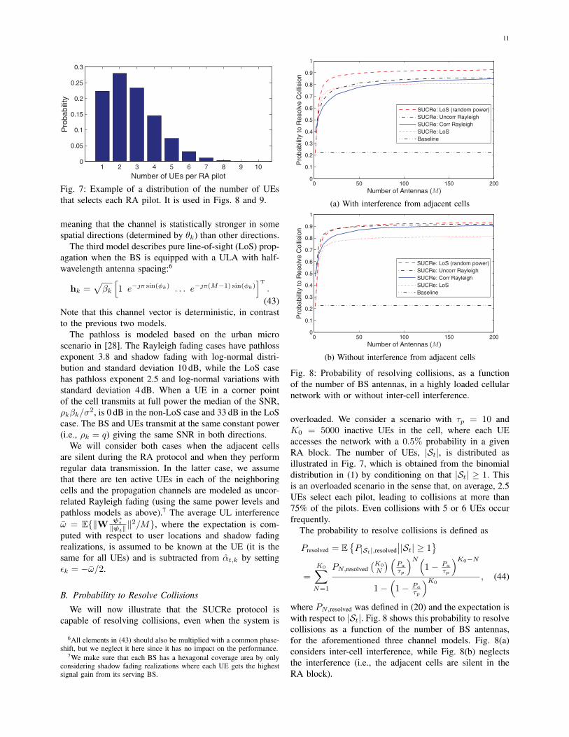
Fig. 8: Probability of resolving collisions, as a functionof the number of BS antennas, in a highly loaded cellularnetwork with or without inter-cell interference.
overloaded. We consider a scenario with τp = 10 andK0 = 5000 inactive UEs in the cell, where each UEaccesses the network with a 0.5% probability in a givenRA block. The number of UEs, |St|, is distributed asillustrated in Fig. 7, which is obtained from the binomialdistribution in (1) by conditioning on that |St| ≥ 1. Thisis an overloaded scenario in the sense that, on average, 2.5UEs select each pilot, leading to collisions at more than75% of the pilots. Even collisions with 5 or 6 UEs occurfrequently.
The probability to resolve collisions is defined as
Presolved = E{P|St|,resolved
∣∣|St| ≥ 1}
=
K0∑N=1
PN,resolved(K0
N
) (Paτp
)N(1− Pa
τp
)K0−N
1−(
1− Paτp
)K0, (44)
where PN,resolved was defined in (20) and the expectation iswith respect to |St|. Fig. 8 shows this probability to resolvecollisions as a function of the number of BS antennas,for the aforementioned three channel models. Fig. 8(a)considers inter-cell interference, while Fig. 8(b) neglectsthe interference (i.e., the adjacent cells are silent in theRA block).

12
The first observation from Fig. 8 is that the SUCReprotocol relies on the channel hardening and favorablepropagation of Massive MIMO channels; Presolved is 20-40% at M = 1, but increases steeply to 75-90% whenhaving M = 50 antennas. The probability to resolvecollisions continues to increase for M ≥ 50, but at aslower pace. Uncorrelated Rayleigh fading gives betterresults than correlated Rayleigh fading, but the differenceis small when M is large. The LoS model has slightlyworse performance, because the pathloss differences arelower which makes it harder to appoint a strongest UE.However, since the cell-edge SNR is higher in the LoS casewe can afford to create SNR differences by randomizingthe UL pilot powers (as discussed in Remark 4). Fig. 8also shows the LoS case when each UE reduces itspilot power with a random number between 0 dB and−30 dB, uniformly distributed in dB-scale. This case givesthe highest performance among all the cases. Hence, theSUCRe protocol is well suited for both LoS and non-LoSchannels.
As a baseline, we also consider a conventional protocolwhere pilot collisions are only handled by retransmissionin later RA blocks. Specifically, using Fig. 1, all UEsdeterministically repeat the pilots in Step 3 of the ac-cess protocol and proceed to the process of centralizedcontention resolution. Fig. 8 shows the probability toresolve collisions and we notice that the SUCRe protocolis able to admit roughly four times as many UEs perRA pilot than the baseline scheme. We also notice thatinter-cell interference only causes a minor degradation inperformance, except in the LoS case where performanceis almost unaffected. The full-power LoS case performssimilarly to the other channel models in this case.
C. Tuning Probabilities using Bias Term
Next, we consider the same scenario but focus onuncorrelated Rayleigh fading channels and study the prob-abilities of resolving collisions, false negatives, and falsepositives. We will demonstrate how the bias term εkcan be utilized to tune the decisions by setting εk =δβk/
√M − ω/2, which corresponds to adding δ standard
deviations of ‖hk‖2/M (around its mean value βk). Fig. 9shows the probabilities as a function of δ, for M = 100and with or without inter-cell interference.
By subtracting one or two standard deviations fromαt,k/2 in the decision rule, we can encourage UE kto appoint itself the contention winner. This leads tohigher probability of resolving collisions, at the cost ofmore false positives where multiple UEs repeat their pilottransmissions in Step 3. In contrast, by adding one ortwo standard deviations to αt,k/2 in the decision rule, wecan discourage UE k from appointing itself the contentionwinner and thereby push the probability of false positivestowards zero—at the cost of resolving fewer collisions and
−2 −1.5 −1 −0.5 0 0.5 1 1.5 20
0.1
0.2
0.3
0.4
0.5
0.6
0.7
0.8
0.9
1
Bias term (in standard deviations)
Pro
babi
lity
Resolved collisionFalse negative (no UEs)False positive (multiple UE)
(a) With interference from adjacent cells
−2 −1.5 −1 −0.5 0 0.5 1 1.5 20
0.1
0.2
0.3
0.4
0.5
0.6
0.7
0.8
0.9
1
Bias term (in standard deviations)
Pro
babi
lity
Resolved collisionFalse negative (no UEs)False positive (multiple UE)
(b) Without interference from adjacent cells
Fig. 9: Probability of resolving collisions, false negatives,and false positives for different bias terms in the decisionrule, for uncorrelated Rayleigh fading channels.
having more false negatives where no UEs repeat theirpilots in Step 3.
The probability of resolving a collision is naturallydecreasing as the number of colliding users increases. Oursimulation results reveal that the SUCRe protocol withδ = −1 resolves 92% of the two-UE collisions, 82% ofthe five-UE collisions, and 71% of ten-UE collisions. Notethat it is unlikely to have more than a handful of collidingUEs per RA pilot, except when the network is extremelyoverloaded.
D. Average Number of RA Attempts in Crowded Scenarios
We have previously shown that the SUCRe protocolcan resolve RA collisions, but the main purpose of anRA protocol is that every UE should be admitted tothe data blocks after as few RA attempts as possible.We study this performance indicator in a scenario withM = 100, τp = 10, and varying number of inactive UEs:K0 ∈ [100, 12000]. Each UE decides to access the networkwith 0.1% probability. If it is not admitted immediately,then in the upcoming blocks the UE joins the SUCReprocess that runs in that block with probability 0.5. Ifthe UE has not succeeded after sending RA pilots in a

13
0 2000 4000 6000 8000 10000 120000
2
4
6
8
10
Number of Inactive UEs
Ave
rage
Num
ber
of A
cces
s A
ttem
pts
SUCRe: No interf.SUCRe: InterferenceBaseline
(a) Average number of RA attempts
0 2000 4000 6000 8000 10000 120000
0.2
0.4
0.6
0.8
1
Number of Inactive UEs
Fra
ctio
n of
Fai
led
Acc
ess
Atte
mpt
s
SUCRe: No interf.SUCRe: InterferenceBaseline
(b) Probability of failed RA attempt (more than 10 attempts)
Fig. 10: RA performance in a cellular network, whereeach UE accesses the network with 0.1% probabilityand sends 10 RA pilots before giving up. The SUCReprotocol can handle substantially higher user loads, K0,than conventional methods.
total of 10 SUCRe processes (including the initial one),then it stops the transmission; that is, it considers thataccess has been denied by the network. Note that theprocedure of joining the 9 additional SUCRe processescan be optimized according to the principles of splittingtree protocols [29], [30], but this optimization is outsidethe scope of this paper. We consider uncorrelated Rayleighfading, cases with and without inter-cell interference, andwe use the bias term εk = −βk/
√M − ω/2. The SUCRe
protocol is compared with the same baseline protocol asbefore (i.e., it only handles collisions by retransmission)with the addition that the UEs make 10 RA attempts atrandom occasions in the same way as the SUCRe protocol.
Fig. 10(a) shows the average number of RA attemptsthat each UE makes, as a function of K0, while Fig. 10(b)shows the fraction of UEs that fails to access the network(i.e., made 10 unsuccessful attempts). The SUCRe protocolcan easily handle up to K0 = 6000 under inter-cellinterference and K0 = 8000 when the adjacent cells aresilent in the RA blocks. For larger values of K0 around0–15% of the UEs will fail to be admitted. Notice that atK0 = 10000 there will on average be K0 · 0.001/τp = 1UE that selects each RA pilot, meaning that the networkis fundamentally overloaded. Nevertheless, an astonishing90% of the UEs can still access the network successfully,which matches well with the 90% probability of resolving
collisions observed in Fig. 8. This behavior remains alsofor K0 > 10000. In contrast, the baseline protocol re-quires more retransmissions when K0 < 3000 and as K0
increases in the range K0 > 3000 the RA functionalitygradually breaks down; at K0 = 10000 only 1.5% of theUEs are successful in their RA attempts.
V. CONCLUSION
The pilot sequences are precious resources in MassiveMIMO since they enable the BS to separate the UEs inthe spatial domain. In future urban scenarios, the numberof UEs that resides in a cell is much larger than thenumber of available pilots, thus the pilots need to betemporally allocated only to the UEs that have data totransmit or receive. The proposed SUCRe random accessprotocol provides an efficient way for UEs to request pilotsfor data transmission, and is well-suited for beyond-LTEMassive MIMO systems and crowded urban deploymentscenarios. The protocol exploits the channel hardeningand favorable propagation properties to enable distributedcollision detection and resolution at the UEs, where thecontender with the strongest signal gain is the one be-ing admitted. The numerical results demonstrate that theSUCRe protocol can resolve around 90% of all collisionsand that it is robust to inter-cell interference and choice ofchannel distribution. The protocol does not break down inoverloaded situations, where more UEs request pilots thanthere are RA resources, but continues to admit a subset ofthe accessing UEs.
APPENDIX ASOME USEFUL RESULTS
Lemma 2 (§8.328.2 in [31]). The Gamma function satis-fies
Γ(M + 1
2
)√MΓ (M)
→ 1 as M →∞. (45)
Lemma 3. For any non-negative integer m and real-valuedA and B, we have∫ ∞
0
xme−(xA−B)2dx
=
m∑n=0
(mn
)Bm−n
Am+1
Γ(n+12 )+(−1)nγ(n+1
2 ,B2)
2 , B ≥ 0,
m∑n=0
(mn
)Bm−n
Am+1
Γ(n+12 )−γ(n+1
2 ,B2)
2 , B < 0.
(46)
Proof: By the change of variable x = x+BA we obtain∫ ∞
0
xme−(xA−B)2dx =
∫ ∞−B
(x+B
A
)me−x
2
Adx
=
m∑n=0
(m
n
)Bm−n
Am+1
∫ ∞−B
xne−x2
dx, (47)

14
where the second equality follows from applying thebinomial formula to (x + B)m. If B ≥ 0, the remainingintegral is computed as∫ ∞−B
xne−x2
dx =
∫ ∞0
xne−x2
dx+ (−1)n∫ B
0
xne−x2
dx
=Γ(n+1
2
)+(−1)nγ(n+1
2 , B2)
2(48)
by making the variable substitution y = x2 and identifyingincomplete gamma functions. Similarly, if B < 0 we have∫ ∞
−Bxne−x
2
dx =
∫ ∞0
xne−x2
dx−∫ −B
0
xne−x2
dx
=Γ(n+1
2
)− γ(n+1
2 , B2)
2. (49)
Substituting (48) or (49) into (47) yield the final result.
APPENDIX BCOLLECTION OF PROOFS
Proof of Lemma 1: Suppose for a moment that Stis known, then the MMSE estimator of hk from theobservation yt at BS 0 is [32]
hk,MMSE =
√ρkτpβk
αt + σ2y. (50)
The true channel can be expressed as hk = hk,MMSE+ek,where the estimate
hk,MMSE ∼ CN(0,ρkτpβ
2k
αt + σ2IM
)(51)
is independent from the estimation error
ek ∼ CN(0,
(βk −
ρkτpβ2k
αt + σ2
)IM
). (52)
The BS does not know St, but we notice that
h∗k,MMSE
‖hk,MMSE‖=
y∗
‖y‖, (53)
thus the received signal in (13) can be rewritten as
zk =√qτph
T
k
h∗k,MMSE
‖hk,MMSE‖+ υT
k
φ∗t‖φt‖
+ ηk
=√qτp‖hk,MMSE‖︸ ︷︷ ︸
=gk
+√qτp
eT
k h∗k,MMSE
‖hk,MMSE‖+ υT
k
φ∗t‖φt‖
+ ηk︸ ︷︷ ︸=νk
, (54)
where we call the two terms gk and νk. We notice that
eT
k h∗k,MMSE
‖hk,MMSE‖∼ CN
(0, βk −
ρkτpβ2k
αt + σ2
)(55)
since ek is independent from the channel estimate andhk,MMSE
‖hk,MMSE‖is uniformly distributed over the unit sphere in
CM . Hence, gk and νk are independent random variables.In addition, νk is the sum of three independent complexGaussian variables which have zero mean and the totalvariance as stated in the lemma. Finally, we notice thatg2k is the sum of squares of 2M independent Gaussian
variables with zero mean and variance 12
ρkqβ2kτ
2p
αt+σ2 , thus gkhas a scaled chi-distribution with 2M degrees of freedomas stated in the lemma.
Proof of Theorem 1: The ML estimator is defined as
α?t,k = arg maxα
f (zk,<, zk,=|α) (56)
where f (zk,<, zk,=|α) is the joint PDF. Since the UEknows that ρkβkτp, it is sufficient to search for α ≥ρkβkτp. Notice that zk,< = gk +<(νk) and zk,= = =(νk)are independent since νk ∼ CN (0, λ2) has independentreal and imaginary parts that are distributed asN (0, λ2/2).Hence,
f (zk,<, zk,=|α) = f1 (zk,<|α) f2 (zk,=|α) (57)
where f2 (zk,=|α) in (31) is the PDF of =(νk). It remainsto compute the PDF f1 (zk,<|α) of zk,<, which is aconvolution of the PDFs of gk and <(νk):
f1 (zk,<|α) =
∫ ∞0
2x2M−1e−x2/λ1
Γ(M)λM1
e−(zk,<−x)2/λ2
√πλ2
dx
=2e−z
2k,</λ2
Γ(M)λM1√πλ2
∫ ∞0
x2M−1e−x2( 1λ1
+ 1λ2
)+x2zk,<λ2 dx
=2e−
(zk,<)2
λ2
(1− λ1
λ1+λ2
)Γ(M)λM1
√πλ2
∫ ∞0
x2M−1e−(xA−B)2dx (58)
where A =√
1λ1
+ 1λ2
and B =zk,<λ2A
. The final expressionfor f1 in (57) is obtained by computing the integral in (58)using Lemma 3 with m = 2M − 1.
Proof of Theorem 2: The probability of repeating thepilot in Step 3, based on (18), is
Pr{Rk} = Pr{
2ρkβkτp > αapprox2t,k + 2εk
}. (59)
Notice that whenever εk < ρkβkτp/2, αapprox2t,k = ρkβkτp
will always lead to pilot repetition, thus we can neglectthe maximum-operator in (36) and write
Pr{Rk} = Pr
{2ρkβkτp > C2
M
qρkβ2kτ
2p
(<(zk))2 − σ
2 + 2εk
}= Pr
{(<(zk))
2> ζk
}(60)
where we use the notation CM = Γ(M+ 1
2
)/Γ (M) and
the second equality follows from rearranging the term and

15
identifying ζk from (38). Since <(zk) can be negative, werewrite (60) as
Pr{Rk} = Pr{<(zk) >
√ζk
}+ Pr
{<(zk) < −
√ζk
}= 1− Pr
{<(zk) ≤
√ζk
}+ Pr
{<(zk) ≤ −
√ζk
}.
(61)
which utilizes the fact that Pr{<(zk) < −√ζk} =
Pr{<(zk) ≤ −√ζk}. It remains to compute the CDF
Pr {<(zk) ≤ d} for an arbitrary d, which is the convo-lution of the CDF of gk and the PDF of <(νk):
Pr{<(zk) ≤ b} =
∫ ∞0
γ(M, x
2
2λ1
)Γ(M)
e−(b−x)2/λ2
√πλ2
dx
=
∫ ∞0
e−(b−x)2/λ2
√πλ2
dx
−∫ ∞
0
e−x2/λ1
M−1∑k=0
x2k
λk1Γ(k + 1)
e−(b−x)2/λ2
√πλ2
dx (62)
by utilizing the definition of the incomplete gamma func-tion (see Footnote 3). The first integral in (62) is over aGaussian PDF and identified as Q(−b
√2/λ2). The second
integral can be rewritten as
M−1∑k=0
e−b2/λ2
Γ(k + 1)λk1√πλ2
∫ ∞0
x2ke−x2( 1λ1
+ 1λ2
)+x 2bλ2 dx
=
M−1∑k=0
e− b2
λ2
(1− λ1
λ1+λ2
)Γ(k + 1)λk1
√πλ2
∫ ∞0
x2ke−(xA−B)2dx (63)
where A =√
1λ1
+ 1λ2
and B = bλ2A
. The final expressionin (39) is obtained from (62)–(63) by computing theremaining integral using Lemma 3 with m = 2k.
Proof of Corollary 1: The Lindeberg-Levy central limittheorem implies that gk converges to N (
√λ1CM , λ
21(M−
C2M )) in distribution as M → ∞, where CM =
Γ(M+ 1
2
)/Γ (M). Since <(zk) = gk + <(νk) converges
to the sum of two independent Gaussian variables (recallLemma 1), the CDF is obtained by (40).
Notice that (37) can be expressed as
Pr{Rk} = 1+Pr{<(zk) >√ζk})−Pr{<(zk) > −
√ζk}.
(64)Since ζk in (38) is positive, Pr{<(zk) > −
√ζk} →
Q(−∞) = 1 as M →∞. Similarly, we notice that
Pr{<(zk) >√ζk})→
1, ζk < C2
Mλ1,
1/2, ζk = C2Mλ1,
0, ζk > C2Mλ1.
(65)
The asymptotic probabilities in (41) follows directly fromthese results.
REFERENCES
[1] Ericsson, “Ericsson mobility report,” Tech. Rep., Nov. 2015.[2] M. Fallgren, B. Timus, et al., D1.1: Scenarios, requirements and
KPIs for 5G mobile and wireless system, ICT-317669-METIS,2013.
[3] F. Boccardi, R. W. Heath, A. Lozano, T. L. Marzetta, andP. Popovski, “Five disruptive technology directions for 5G,” IEEECommun. Mag., vol. 52, no. 2, pp. 74–80, 2014.
[4] T. L. Marzetta, “Noncooperative cellular wireless with unlimitednumbers of base station antennas,” IEEE Trans. Wireless Commun.,vol. 9, no. 11, pp. 3590–3600, 2010.
[5] E. Bjornson, E. G. Larsson, and M. Debbah, “Massive MIMO formaximal spectral efficiency: How many users and pilots should beallocated?,” IEEE Trans. Wireless Commun., vol. 15, no. 2, pp.1293–1308, 2016.
[6] E. Bjornson, E. G. Larsson, and T. L. Marzetta, “Massive MIMO:Ten myths and one critical question,” IEEE Commun. Mag., vol.54, no. 2, pp. 114–123, Feb. 2016.
[7] J. Vieira, S. Malkowsky, K. Nieman, Z. Miers, N. Kundargi, L. Liu,I. C. Wong, V. Owall, O. Edfors, and F. Tufvesson, “A flexible100-antenna testbed for massive MIMO,” in Proc. IEEE GlobecomWorkshop - Massive MIMO: From Theory to Practice, 2014.
[8] J. Jose, A. Ashikhmin, T. L. Marzetta, and S. Vishwanath, “Pilotcontamination and precoding in multi-cell TDD systems,” IEEETrans. Commun., vol. 10, no. 8, pp. 2640–2651, 2011.
[9] H. Huh, G. Caire, H. C. Papadopoulos, and S. A. Ramprashad,“Achieving “massive MIMO” spectral efficiency with a not-so-largenumber of antennas,” IEEE Trans. Wireless Commun., vol. 11, no.9, pp. 3226–3239, 2012.
[10] J. Hoydis, S. ten Brink, and M. Debbah, “Massive MIMO in theUL/DL of cellular networks: How many antennas do we need?,”IEEE J. Sel. Areas Commun., vol. 31, no. 2, pp. 160–171, 2013.
[11] H. Ngo, E. Larsson, and T. Marzetta, “Energy and spectralefficiency of very large multiuser MIMO systems,” IEEE Trans.Commun., vol. 61, no. 4, pp. 1436–1449, 2013.
[12] H. Yin, D. Gesbert, M. Filippou, and Y. Liu, “A coordinatedapproach to channel estimation in large-scale multiple-antennasystems,” IEEE J. Sel. Areas Commun., vol. 31, no. 2, pp. 264–273,2013.
[13] A. Adhikary, J. Nam, J.-Y. Ahn, and G. Caire, “Joint spatial divisionand multiplexing—the large-scale array regime,” IEEE Trans. Inf.Theory, vol. 59, no. 10, pp. 6441–6463, 2013.
[14] E. Bjornson, J. Hoydis, M. Kountouris, and M. Debbah, “MassiveMIMO systems with non-ideal hardware: Energy efficiency, esti-mation, and capacity limits,” IEEE Trans. Inf. Theory, vol. 60, no.11, pp. 7112–7139, 2014.
[15] L. Lu, G. Li, A. L. Swindlehurst, A. Ashikhmin, and R. Zhang,“An overview of massive MIMO: Benefits and challenges,” IEEEJ. Sel. Topics Signal Process., vol. 8, no. 5, pp. 742–758, 2014.
[16] E. Bjornson and E. G. Larsson, “Three practical aspects ofmassive MIMO: Intermittent user activity, pilot synchronism, andasymmetric deployment,” in IEEE Globecom Workshops, 2015.
[17] M. Hasan, E. Hossain, and D. Niyato, “Random access formachine-to-machine communication in LTE-advanced networks:Issues and approaches,” IEEE Commun. Mag., vol. 51, no. 6, pp.86–93, 2013.
[18] N. K. Pratas, H. Thomsen, C. Stefanovic, and P. Popovski, “Code-expanded random access for machine-type communications,” inIEEE Globecom Workshops, 2012, pp. 1681–1686.
[19] J. H. Sørensen, E. de Carvalho, and P. Popovski, “Massive MIMOfor crowd scenarios: A solution based on random access,” in IEEEGlobecom Workshops, 2014, pp. 352–357.
[20] E. de Carvalho, E. Bjornson, E. G. Larsson, and P. Popovski,“Random access for massive MIMO systems with intra-cell pilotcontamination,” in Proc. IEEE ICASSP, 2016.
[21] L. Sanguinetti, A. A. D’Amico, M. Morelli, and M. Debbah,“Random access in uplink massive MIMO systems: How to exploitasynchronicity and excess antennas,” in IEEE GLOBECOM, 2016.
[22] E. Paolini, G. Liva, and M. Chiani, “High throughput random accessvia codes on graphs: Coded slotted ALOHA,” in IEEE InternationalConference on Communications (ICC), 2011, pp. 1–6.

16
[23] E. Paolini, C. Stefanovic, G. Liva, and P. Popovski, “Coded randomaccess: How coding theory helps to build random access protocols,”IEEE Commun. Mag., vol. 53, no. 6, pp. 144–150, June 2015.
[24] E. Bjornson, E. de Carvalho, E. G. Larsson, and P. Popovski, “Ran-dom access protocol for massive MIMO: Strongest-user collisionresolution (SUCR),” in Proc. IEEE ICC, 2016.
[25] H. Ngo, E. Larsson, and T. Marzetta, “Aspects of favorablepropagation in massive MIMO,” in Proc. EUSIPCO, 2014.
[26] R. Couillet and M. Debbah, Random Matrix Methods for WirelessCommunications, Cambridge University Press, 2011.
[27] S. L. Loyka, “Channel capacity of MIMO architecture using theexponential correlation matrix,” IEEE Commun. Lett., vol. 5, no.9, pp. 369–371, 2001.
[28] Spatial channel model for Multiple Input Multiple Output (MIMO)simulations (Release 13), 3GPP TR 25.996, Dec. 2015.
[29] J. I. Capetanakis, “Tree algorithms for packet broadcast channels,”IEEE Trans. Inf. Theory, vol. 25, no. 5, pp. 505–515, 1979.
[30] J. H. Sørensen, C. Stefanovic, and P. Popovski, “Coded splittingtree protocols,” in IEEE ISIT, 2013, pp. 2860–2864.
[31] I. S. Gradshteyn and I. M. Ryzhik, Table of Integrals, Series, andProducts, Academic Press, 1980.
[32] S. M. Kay, Fundamentals of Statistical Signal Processing: Estima-tion Theory, Prentice Hall, 1993.