A R Adaptive Multiple Importance Sampling (ARAMIS)

Luca Pozzi, University of California, Berkeley, U.S.A.Antonietta Mira, University of Lugano, Lugano, Switzerland

Modified: November 9th, 2012, Compiled: January 21, 2013

Abstract

ARAMIS is an R package that runs the AMIS [1] algorithm. The main features of ARAMIS areparallelization and customization.ARAMIS exploits the massively parallel structure of AMIS to improve the performance of the algorithm asit was implemented in the original paper. As a result simulation time is reduced by orders of magnitudes.

As for customization, the potential of the R language is fully exploited by ARAMIS which allows theuser to taylor the software to the model which results from his or her own research setting. Target andproposal kernel can be easily specified by the user. Some working examples contained in the manualexplain how this can be efficiently and easily done.

As a consequence of the flexibility and efficiency of the package, even fairly complicated problems canbe accommodated, e.g. sampling from an Extreme Value (EV) Copula distribution with a mixture ofEV distributions as the proposal kernel. The latter is an interesting and useful example of how the usercan specify some “real-world” combination of target/proposal and it is added, in the manual, to the twoworking examples detailed in [1].

1 Introduction

ARAMIS is an R package that runs AMIS [1], an Adaptive Multiple Importance Sampler that uses a setof particles that evolve over an artificial time dimension. The particles are generated from an importancedistribution and, properly weighted, provide a representation of (a sample from) the target distribution, astypically done in Importance Sampling (IS). What distinguishes AMIS from the other IS algorithms is thatold (i.e. generated at earlier times) particles are exploited to adaptively design the importance distributionin the same spirit of Adaptive Markov Chain Monte Carlo (AMCMC) where the proposal distribution is“adapted” instead. The main difference from classic AMCMC, is that in this class time is a natural parameter(i.e. the evolution time of the stochastic process generated by the Metropolis-Hastings algorithm) and toeach sample (that form the simulated path of the “Markov” chain), there is no associated importance weight.We can thus define AMIS as an hybrid between AMCMC and IS: exploiting the best from both strategiesresulting in an efficient sampler with good performance also in high dimensions as proved in [1].

The main features of ARAMIS are parallelization and customization.

Parallel implementation: by its nature AMIS shows a embarrassingly parallel structure which is exploitedby ARAMIS to improve the performance of the algorithm and reduce simulation time by orders of mag-nitudes relative to its original implementation in [1]. Following a Map-Reduce scheme the computationsare sent to the independent computing units and then the results are collected and merged together.Each core takes care of an approximately equal set of particles evaluating the importance weights andmerging them together to compute the new IS estimates at each iteration of the algorithm. Thus, thereduction in computational tim is directly proportional to the number of particles used in the under-lying Importance Sampler.The musketeers slogan “all for one andone for all” can be re-interpreted in light of the parallel featuresor ARAMIS that make it an hard to beat software to sample from complicated and high dimensionaltarget distributions.

1

Customization: the potential of the R language is fully exploited by ARAMIS which allows the user totaylor the software to the model which results from his or her own research setting. Target and proposalkernel can be easily specified by the user.

As a consequence of the flexibility of the package, even fairly complicated problems can be accommodated,e.g. sampling from a Copula distribution with a mixture of extreme value distribution as the proposal kernel.The latter is an interesting and useful example of how the user can specify some “real-world” combinationof target/proposal and it is added, in the manual, to the two working examples detailed in [1]. Very littlead-hoc code is needed to sample an extreme value copula distribution: package “copula” provides a way toevaluate the target distribution and package “evd” offers useful tools for extreme value distributions whichare easily plugged in the ARAMIS function. This is explained extensively in Section 5

2 Adaptive Multiple Importance Sampling (AMIS)

Given a density π known up to a normalizing constant, and a function h, interest is in computing

Π(h) =

∫h(x)π(x)µ(dx) =

∫h(x)π̃(x)µ(dx)∫π̃(x)µ(dx)

when∫h(x)π̃(x)µ(dx) is intractable. As an alternative to Metropolis-Hastings type algorithms, to estimate

Π(h) one can rely on Importance Sampling strategies. An iid sample x1, . . . , xN ∼ Q is generated from animportance distribution Q, s.t. Q(dx) = q(x)µ(dx) and Π(h) is estimated by

Π̂ISQ,N (h) = N−1

N∑i=1

h(xi){π/q}(xi)

The IS estimator relies on alternative representation of Π(h):

Π(h) =

∫h(x){π/q}(x)q(x)µ(dx)

IS can be generalized to encompass much more adaptive/local schemes than thought previously. Adap-tivity means learning from experience, i.e., designing new IS distributions based on the performances ofearlier ones. The intuition of the AMIS algorithm is, indeed, to use previous sample(s) to learn about π andconstruct cleaver importance distributions q in the same spirit as adaptive MCMC where cleaver proposaldistributions are designed based on the past history of simulated stochastic process.

Following is a description of the AMIS algorithm as it appears in [1]. The algorithm starts with aninitialization phase whose rationale is to provide a good scaling for the initial importance distribution, Q0.

Step 0 - Initialization : (N0 particles, t = 0)

• generate a single set of N0 iid uniforms in U⊗p[0,1];

• with scaled logistic transformation go back to <p;

• compute IS weights as function of the scale, τ , of the logistic distribution;

• use ESS(w) to find a “good” proposal initial scaling (as an alternative, use ESS + tempering);

This initial step is computationally very cheap and automatic.

Step 1 - Adaptation : (N1 particles, t = 1 · · ·T1)The rationale of this step is global adaptation of the parameters of the importance distribution. Thiscan be achieved either by plain adaptation (Step 1) or by combining adaptation with a variancereduction technique introduced to prevent IS weights impoverishment by [3] (Step 1∗).

A potential problem when implementing Step 1 is high variability of the importance weights. This canbe solved implementing, instead, Step 1∗.

2

Step 1∗ - Adaptation plus Variance reduction. The rationale of this step is twofold: Ensure that allparticles are on the same “weighting scale” and can thus be easily and efficiently combined to get finalestimator; Ensure variance reduction thanks to weights stabilization.

Step 2 - Clustering : (N2 particles, t = T1 + 1 · · ·T2)At iteration t = T1 + 1, · · · , T2, for 1 ≤ i ≤ N2:

1. Run Rao–Blackwellised clustering algorithm based on (possibly trimmed by resample) pastparticles using a mixture of Gaussian distributions to cluster. The number of components, G, ischosen by BIC.

2. Estimate the mean, µ̂g, and the covariance Σ̂g, on each cluster g.

3. Simulate new sample xt+11 , . . . , xt+1

n from p-variate mixture (G components) of T(3)(µ̂g, Σ̂g).

4. For i = 1, . . . , N compute weights ωT+1i of particle xT+1

i using Deterministic Mixture idea.

5. For 1 ≤ l ≤ T , actualize past importance weights.

The final AMIS estimator recycles all [N0] + [N1 × T1] + [N2 × (T2 − T1)] generated particles with thecorresponding importance weights. This is done to avoid waste of particles and to combine global (step 1)and local adaptation (step 2).

The resulting AMIS algorithm is user friendly, provides an unbiased estimator of integrals with respectto the target and is highly efficient requiring no tuning, allowing for automatic local and global adaptationof the importance distribution. The algorithm is multi-purpose, interruptible and requires no burn-in (un-like AMCMC) and, as simulation proceeds, updates both the weights and the parameters of the mixtureimportance distribution.

3 ARAMIS Basics: Inputs, Outputs and Help of ARAMIS

The structure of AMIS naturally leads to require the following inputs (to be specified by the user), forARAMIS:

Inputs (to be specified by the user):

• the size of the population both in the initialization, global and local adaptation phase

• the length of the simulation in the global and local adaptation phase

• the target distribution

• the kernel used in the importance distribution (whose parameters are adapted as the simula-tion proceeds): the default kernel is a non-central T-distribution with 3 degrees of freedom (assuggested in [1]).

Outputs Upon running ARAMIS the following output is obtained:

• generated samples and corresponding importance weights

• effective sample size (a measure of the algorithm performance introduced in Section 4.1 of [2]))

• mean and variance covariance matrix of the target distribution estimated by importance sampling

Help an on-line help is available with three examples worked out in details to guide the user: two are takenform the original paper [1]) (a banana-shaped and a mixture distribution target), while the last one isan original example where the target is a multivariate Extreme Value (EV) distribution obtained by aCopula construction.

3

4 First Steps with ARAMIS

Let’s start by loading the package

> library(ARAMIS)

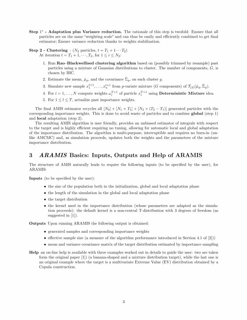
As a first example let’s run an Adaptive Importance Sampling (i.e. the scheme in which the weights don’tget actualized), on a “Banana”-shaped target distribution which is defined as follows:

• start with a p-dimensional Gaussian

(x1, ..., xp) ∼ Np(0, diag(100, 1, ..., 1))

• change the second coordinate to

y2 = x2 + bx21 − 100b

for some “Banana”-ness coeficient b which is set by default to b = 0.03.

> ais <- AIS(N=1000,

+ niter=10,

+ p=2,

+ target= targetBanana(),

+ initialize=uniInit(),

+ mixture= mclustMix())

−30 −10 10 30

−30

−20

−10

010

2030

AIS Algorithm; targetBanana Target

x1

x 2

x[1]

x[2]

target

AIS Algorithm; targetBanana Target

4

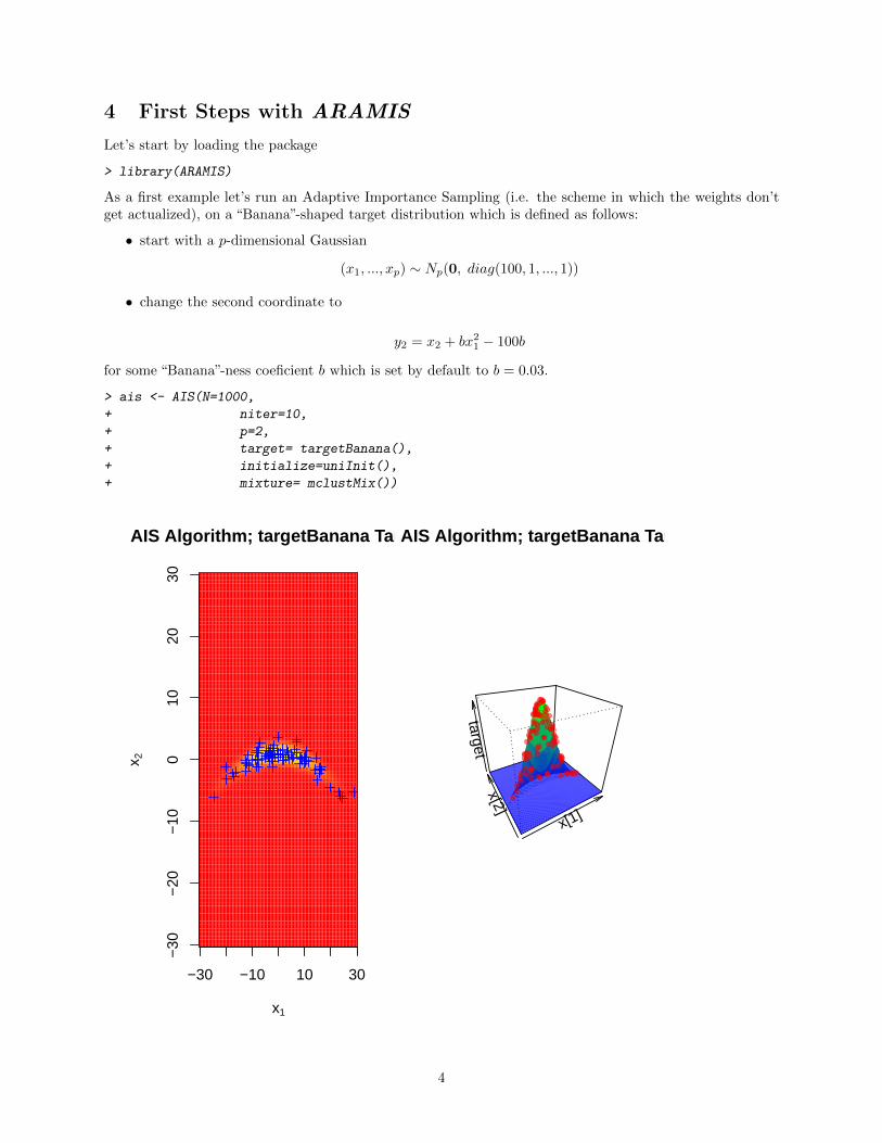
Let’s now try the AMIS algorithm on a even stronger shaped Banana target (b = 0.1, which implies amuch harder target)

> amis <- AMIS(N=1000,

+ niter=10,

+ p=2,

+ target=targetBanana(b=0.1),

+ initialize= amisInit(maxit=5000),

+ mixture=mclustMix())

−30 −10 10 30

−30

−20

−10

010

2030

AMIS Algorithm; targetBanana TargetAMIS Algorithm; 0.1 Target

x1

x 2

x[1]

x[2]

target

AMIS Algorithm; targetBanana TargetAMIS Algorithm; 0.1 Target

The ISO object returned by the function contains the sample from the target distribution and somefurther useful information.

> showClass("ISO")

Class "ISO" [package "ARAMIS"]

Slots:

Name: IS Prop Mean Var Perp ESS

Class: matrix numeric matrix array numeric numeric

Name: seed envir call args

Class: integer environment call list

5

> summary(amis)

Call:

AMIS(N = 1000, niter = 10, p = 2, target = targetBanana(b = 0.1),

initialize = amisInit(maxit = 5000), mixture = mclustMix())

Global ESS: 763.7322

Maximum Perplexity: 0.8668435

ISO objects allow the use of familiar syntax

> amis$ESS

[1] 763.7322

> ais[["ESS"]]

[1] 9009.858

but have also other useful methods, like plot, mean and var: let’s use them for a simple sanity check:

x1 x2

125.2236 448.2367

x1 x2

x1 125.38778 18.07847

x2 18.07847 448.82438

5 How to use ARAMIS for your Research

The purpose of this section is to illustrate the functionality of the package on a real world example and tobriefly show how the algorithm can be personalized to respond to your needs.

The algorithm is written in a general form so that the user can specify his favorite combination of targetdistribution, component of the proposal distribution and clustering algorithm, the way to really exploit allthe flexibility is to use the technique called function closure.

To illustrate the use of function closures let’s try the algorithm on a hard-to-tackle-problem. Let’s use asa target the following Galambos copula

> # Galambos Copula

> # a : location parameter GEV

> # b : scale parameter GEV

> # s : shape parameter GEV

> # theta : copula's parameter

>

> galambosCop <- function(a=0,b=1,s=0,theta=1.5,copula=galambosCopula){

+

+ require("copula")

+ require("evd")

+

+ Cop <- copula(theta)

+

+ function(xx){

+

+ U <- pgev(xx,loc=a, scale=b,shape=s)

+ # numerical stability can be a issue...

+ U[U>1-sqrt(.Machine$double.eps)] <- 1-sqrt(.Machine$double.eps)

6

+ U[U<sqrt(.Machine$double.eps)] <- sqrt(.Machine$double.eps)

+

+ if(length(dim(xx)>1)){

+ trgt <- log(dCopula(U,Cop))+

+ rowSums(apply(xx,2,function(x)

+ dgev(x,loc=a, scale=b,shape = s,log=TRUE)))

+ }else{

+ trgt <- log(dCopula(U,Cop))+

+ sum(dgev(xx,loc=a, scale=b,shape=s,log=TRUE))

+ }

+

+ trgt

+

+ }

+ }

This is what the function closure consists into: to build an environment around the function that containsall the parameters the function needs but that are not being passed as an argument. This allows us to makethe list of arguments completely general, in the example a, b, s, etc... are enclosed in scope of the function

> toughCop <- galambosCop()

> ls(envir=environment(toughCop))

[1] "Cop" "a" "b" "copula" "s" "theta"

> get("theta",envir=environment(toughCop))

[1] 1.5

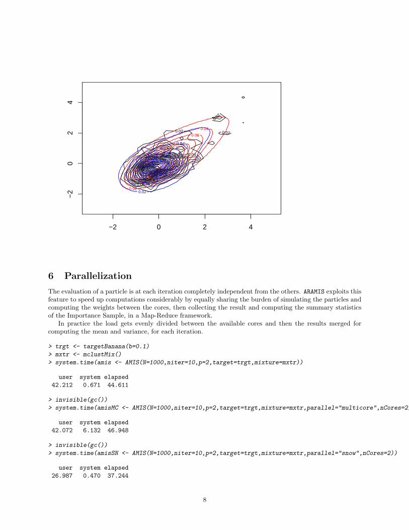
We can now run AMIS and see from the plot how this is fully captured by the algorithm.

> resCop <- AMIS(N=c(500,1000,500),

+ niter=c(10,50),

+ p=2,

+ target=toughCop,

+ initialize= amisInit(maxit=5000),

+ mixture=mclustMix())

> plot(resCop,whichOne=3L, xlim=c(-3,5),ylim=c(-3,5),N=17000)

>

7

0.02

0.04

0.06

0.08

0.1 0.12

0.14

0.16

0.18 0.2

−2 0 2 4

−2

02

4

0.02

0.04

0.06

0.08

0.1

0.12

0.14 0.1

6

0.18

0.26

0.28

0.02

0.02

0.02

0.04

0.06

0.08 0.1

0.12 0

.14

0.1

6

0.22

0.26

6 Parallelization

The evaluation of a particle is at each iteration completely independent from the others. ARAMIS exploits thisfeature to speed up computations considerably by equally sharing the burden of simulating the particles andcomputing the weights between the cores, then collecting the result and computing the summary statisticsof the Importance Sample, in a Map-Reduce framework.

In practice the load gets evenly divided between the available cores and then the results merged forcomputing the mean and variance, for each iteration.

> trgt <- targetBanana(b=0.1)

> mxtr <- mclustMix()

> system.time(amis <- AMIS(N=1000,niter=10,p=2,target=trgt,mixture=mxtr))

user system elapsed

42.212 0.671 44.611

> invisible(gc())

> system.time(amisMC <- AMIS(N=1000,niter=10,p=2,target=trgt,mixture=mxtr,parallel="multicore",nCores=2))

user system elapsed

42.072 6.132 46.948

> invisible(gc())

> system.time(amisSN <- AMIS(N=1000,niter=10,p=2,target=trgt,mixture=mxtr,parallel="snow",nCores=2))

user system elapsed

26.987 0.470 37.244

8

> summary(amis)

Call:

AMIS(N = 1000, niter = 10, p = 2, target = trgt, mixture = mxtr)

Global ESS: 823.0445

Maximum Perplexity: 0.8766368

> summary(amisMC)

Call:

AMIS(N = 1000, niter = 10, p = 2, target = trgt, mixture = mxtr,

parallel = "multicore", nCores = 2)

Global ESS: 921.6402

Maximum Perplexity: 0.9197068

> summary(amisSN)

Call:

AMIS(N = 1000, niter = 10, p = 2, target = trgt, mixture = mxtr,

parallel = "snow", nCores = 2)

Global ESS: 783.0711

Maximum Perplexity: 0.8846833

> par(mfrow=c(1,3))

> plot(amis,whichOne=1L)

> plot(amisMC,whichOne=1L)

> plot(amisSN,whichOne=1L)

>

−30 −10 10 30

−30

−20

−10

010

2030

AMIS Algorithm; trgt Target

x1

x 2

−30 −10 10 30

−30

−20

−10

010

2030

AMIS Algorithm; trgt Target

x1

x 2

−30 −10 10 30

−30

−20

−10

010

2030

AMIS Algorithm; trgt Target

x1

x 2

9

Acknowledgments

We thank J.M. Marin for providing the code to run the AMIS algorithm on the examples of the paper [1]and M. Garieri for helping with many computational issues and frustrations.

References

[1] Cornuet, J.M. and Marin, J.M. and Mira, A. and Robert,C. Adaptive Multiple Importance Sampling.Scandinavian Journal of Statistics (2012).

[2] Liu, J. and Chen, R. Blind Deconvolution via Sequential Imputations. Journal of the American StatisticalAssociation (1995).

[3] Owen, A. and Zhou, Y. Safe and Effective Importance Sampling. Journal of the American StatisticalAssociation (2000).

[4] Gareth, O. and Roberts,C. and. Rosenthal, J.S.. Examples of Adaptive MCMC. Journal of Computa-tional and Graphical Statistics (2009).

[5] Tierney L. and Mira A. Some Adaptive Monte Carlo Methods for Bayesian Inference. Statistics inMedicine (1999).

SessionInfo

• R Under development (unstable) (2013-01-16 r61667), x86_64-apple-darwin9.8.0

• Locale: C/en_US.UTF-8/en_US.UTF-8/C/en_US.UTF-8/en_US.UTF-8

• Base packages: base, datasets, grDevices, graphics, methods, parallel, stats, utils

• Other packages: ARAMIS 1.0.1, LearnBayes 2.12, MASS 7.3-23, copula 0.999-5, evd 2.3-0, mclust 4.0

• Loaded via a namespace (and not attached): ADGofTest 0.3, gsl 1.9-9, mvtnorm 0.9-9994,pspline 1.0-14, stabledist 0.6-5, stats4 3.0.0, tools 3.0.0

10