A Quick Introduction to R (for Stata Users)

Richard Blissett

September 30, 2016

The following document was originally developed as a quick introduction to R for PhD students at Peabody College,Vanderbilt University. This document assumes very little except (a) a background in Stata, (b) a openness to otherways of thinking about code and data, and (c) a willingness to have fun, be yourself, and explore things you’d liketo learn more about. The examples in this document use the apidata 2012 so.dta dataset, which is included. Thesedata are a subset of 2012 school district achievement data from California’s Academic Performance Index system.

1 Why R?

R is a programming language and environment used primarily for statistical computing. Nearly everything thatStata does, R is able to do. There are benefits and drawbacks to choosing any programming language over another.Being an R tutorial, the bias here is towards R. There are many advantages that R has over Stata.

• R is free. Everyone likes free stuff. Except hotel soap. No one likes hotel soap.

• In R, you can hold multiple datasets open at the same time, which means no more opening and closing andpreserving and restoring datasets to access different data.

• As a result of the above point, it is not always necessary to merge data.

• R is particularly good at producing high-quality graphics (see the R Graph Gallery online for examples).

• All R functions, as well as functions in most other programming languages, have the same basic syntacticalstructure. Stata is fairly unusual in its structure, which has main arguments on one side of a comma andoptions on the other, with frequent confusion by users about what goes where. (Note: By ”frequent confusionby users,” I mean ”frequent confusion by me,” but I’m the one writing this tutorial, so you will just have toaccept my social generalizations.)

• R is highly extensible, meaning that is is very simple for users anywhere in the world to cook up solutions forproblems they face and publish them for anyone to use.

• R can be used in conjunction with other languages fairly easily, including with markup languages like LATEX(thisdocument was created this way).

• The popularity of and interest in R has grown substantially in recent years. See the following for some data onthis point: http://r4stats.com/articles/popularity/

• In terms of one’s growth as a fulfilled and eternal human being, R is closer to other programming languagesoutside of the statistical world. Once you’ve learned R, transitioning to other typical languages such as C,Python, and Java is much easier than if you have jumped straight from Stata.

That all being said, the R vs. Stata vs. any other programming language “debate” is about as clear and useful asthe Mac vs. PC debate. In the end, both are good languages to know. If anything, knowing more than one languagehelps you communicate with other people, and understanding how multiple languages work can help you be morecreative in the work you do and make you the most interesting person at a party.1

1The author is not liable for any social harms incurred by the reader as a result of their attempt to use their knowledge of Stata andR to be the coolest person at a party.

1

1.1 R and RStudio

R can be downloaded from www.rproject.org, where you should click on “CRAN” on the side to download. Followthe on-screen instructions to install.

What you are downloading is the R language as well as basic software that you can use to work in R (like Stata’sgraphical user interface). There are, however, other options (many, in fact) to use R. The one recommended for thistutorial and one that is widely used is RStudio, available from www.rstudio.com. You should still download R fromthe CRAN first, and then download RStudio. When you’ve finally installed RStudio, open it up, and then go to“File > New File > R Script” to open a new editing window.

When you open RStudio, you should have four basic areas on your screen:

1. The top-left is where you type source code, like the script editor in Stata.

2. The bottom-left is the console, where you see what R is doing. Like in Stata, you can just type in the consolenext to the > character.

3. The upper-right is where you see you list of R objects and things in your workspace (explained in the nextsection). History is also there.

4. The bottom right is where you can see your file structure, graphical output, available packages, and helpdocuments.

Console To work in the console, just click anywhere in the console and type away. For example, type “1” and pressenter. You should see something like the following. (In this tutorial, input is colored blue, and output is colored red.)

> 1

[1] 1

Very exciting, yes. For now, though, note that you did not, as you do in Stata, have to type display 1 to get thatback. As long as you are working in this R environment, you wont have to type display to show things (this is notthe case when running R from other scripts, but that is beyond the scope of this document).

Type “1+1” and see what happens. More excitement. I was once told that the R environment was basically a glorifiedcalculator. Years later, I think this comment is still right. Also, remember that in Stata, to scroll through previouscommands, you use the “Page Up” and “Page Down” keys. In the RStudio environment, the up and down arrow keyswill do the same.

R code is written in the source window (upper-left) and saved as a .r file. (Note that RStudio can also edit othertypes of files.) Type and save code here as you would have in Stata.

2

To run a particular line or highlighted block of lines, click the “Run” button at the top of the window. To run theentire script, click “Source.” To run the entire script and see output as you do so, click “Source with Echo.”

2 R Resources

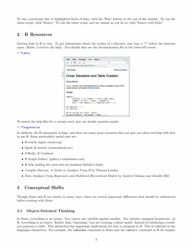
Getting help in R is easy. To get information about the syntax of a function, just type a “?” before the functionname. Below, I retrieve the help . You should then see the documentation file in the lower-left screen.

> ?table

To search the help files for a certain word, just use double question marks.

> ??regression

In addition, the R community is huge, and there are many great resources that can give you ideas and help with howto use R. Some particularly useful ones are:

• R search engine (rseek.org)

• Quick R website (statmethods.net)

• O’Reilly R Cookbook

• R Graph Gallery (gallery.r-enthusiasts.com)

• R help mailing list (stat.ethz.ch/mailman/listinfo/r-help)

• Complex Surveys: A Guide to Analysis Using R by Thomas Lumley

• Data Analysis Using Regression and Multilevel/Hierarchical Models by Andrew Gelman and Jennifer Hill

3 Conceptual Shifts

Though Stata and R are similar in many ways, there are several important differences that should be understoodbefore starting with Stata.

3.1 Object-Oriented Thinking

In Stata, everything is an action. You regress one variable against another. You tabulate marginal frequencies. InR, everything is an object. Rather than “regressing,” you are creating a linear model. Instead of tabulating a result,you generate a table. This distinction has important implications for how to program in R. This is reflected in thelanguages themselves. For example, the tabulate command in Stata and the table() command in R do roughly

3

the same thing for variables in datasets, but note how the command is a verb in Stata and a noun in R. In fact,when you run table() in R, you are actually creating a table “object.”

In Stata, we tend to think of the environment being the data itself, with everything else in Stata being things we“do” to the data. Anything else you store is kept in locals, estimates, and scalars, which are typically temporary andare cleared when your code exits.

Using Stata terminology, imagine that everything is a local. The data is in a local. The regression you just estimatedis a local. In R, the data is only a “thing” in the environment. If you want to run a regression, R essentially createsa regression object, which you can store as another “thing” in your workspace.

R requires a real understanding of how information is stored. When regression estimates are stored in Stata, forexample, we are often not particularly concerned about how the data is stored as long as we can recall it whennecessary. Working creatively in R will require consideration of how this information is stored (an illustration of thisis in the section on regression).

It is because of the object-oriented nature of R that you are able to keep multiple datasets open at the same time.When you open a dataset, you store it in a data frame object. You can have as many objects as your memory allows.As noted before, this can occasionally preclude the need for merging.

This does mean, however, that you have to think of variables as belonging to different datasets, and most of thetime, when using variables, you have to reference which dataset they come from using the $ symbol. (This can beavoided by using the attach() function, which will be discussed later.) For example, the full name of the grades 2-8Engligh score variable within the api dataset would be api$cst28_engl.

3.2 Function Syntax

All functions (commands) are written the same in R:

> functionname(part1, part2, part3)

On other words, every function, in following with our object-oriented thinking, is made up of “parts” which includedata and options. For example, a regression is made up of data, a formula, weights, etc. This is somewhat differentthan functional syntax in Stata, where“main parts”and“options”are separated by a comma, and how the parametersare included differs from function to function.

3.3 Libraries

R comes with a base set of functions, but there are many others that have been written by people to perform moreadvanced tasks. Like Stata’s .ado files, these are written by users and distributed for public use. In R, however, youmust indicate when you are using an external package. This is done as follows:

> library(libraryname)

There are a number of packages that come with your R installation. You can download others by using the in-

stall.packages() command or by going to Tools > Install Packages... in RStudio. It is customary to placeall library() commands at the top of the script.

4 Objects and Basic R

An R object is just information, and it is how information is stored in R. A data table is an object. A regression isan object.

Objects are created when the output from functions are stored within them. The rules for object names are similarto the rules for variable names in Stata (e.g., no special characters, cannot start with a number). To remove anobject, use the rm() command. The following command will clear all objects.

> rm(list=ls())

4

Above, the rm() function is being instructed to remove a list of objects. That list is obtained from the ls() command,which returns a list of all objects currently in your workspace.

4.1 Assignment

Assignment is how you put things into objects. Assignment isn’t such a big deal in Stata unless you work exclusivelyin locals, estimate storage, and scalars (which all are assigned differently). In R, however, assignment is crucial.

In R, type the number 2.

> 2

[1] 2

(Note the [1] before the number. You can ignore that for now.)

If you wanted that 2 to be stored, you would assign it to an object, say, a.

> a <- 2

You can also use the “=” sign to do assignment, but it is generally not recommended in R because of its limitations(not overly critical for early R users).

If you want to see what is in a, just type it.

> a

[1] 2

The same applies for functional output. For example, the sqrt() function takes the square root of a number. So...

> sqrt(a)

[1] 1.414214

> a

[1] 2

Note that the value stored in a did not change. The sqrt() function just did the operation and gave you the outputon the screen. If you wanted to save that, you would do...

> b <- sqrt(a)

> b

[1] 1.414214

Here, the square root was stored in the b object, and not sent to the screen. Note that you also could have overwrittenwhat was in a by assigning sqrt(a) to a itself. R will evaluate the expression to the right of <- and store the outputin the object to the left.

If you wanted to see the output as well, just put parentheses around the command as follows.

> (b <- sqrt(a))

[1] 1.414214

4.2 Basic Math

All basic math is the same in R as it is in Stata (using the +, -, *, and / operators). You can use objects in mathas well.

> a <- 2

> b <- 4

> 2+4

[1] 6

5

> a+b

[1] 6

Math follows the normal order of operations. Functions like log() and sqrt() also exist.

4.3 Lists

In R, to create a list of things, you use the c() function, which stands for combine.

> c(1, 2, 3, 4, 5)

[1] 1 2 3 4 5

This created a list, which you can see. But you didn’t store it, so you can’t call it back if you need that. You canstore it and then see it the same way we just did above. List items can be accessed using bracket notation.2

Also, note that the sequence operator is : (as opposed to / in Stata).

> list <- 1:5

> list

[1] 1 2 3 4 5

> list[1]

[1] 1

Note again that when you assign something to an object, it doesn’t show any output. If you want to see the outputas well, just put parentheses around the line.

> (list <- c(1, 2, 3, 4, 5))

[1] 1 2 3 4 5

You can create lists of objects as well, which may be lists themselves.

> a <- c(1, 2, 3, 4, 5)

> b <- 12

> combine1 <- c(a, b)

> combine1

[1] 1 2 3 4 5 12

> c <- "fish"

> combine2 <- c(combine1, c)

> combine2

[1] "1" "2" "3" "4" "5" "12" "fish"

Note that when you combine numeric types and string types, they all get changed to strings.

5 Control Structures

The function of R’s control structures (e.g. if, while, foreach) are the same as those in Stata.

5.1 If

Below is an example of an if statement.

2If you have previous programming experience, note that unline many other languages, list indices start at 1 rather than 0.

6

> a <- 2

> if(a==2) {

+ print("HEY")

+ } else if(a==3) {

+ print("HELLO")

+ }

[1] "HEY"

5.2 While

Below is an example of a while statement.

> a <- 1

> while(a <= 5) {

+ print("Fish")

+ a <- a + 1

+ }

[1] "Fish"

[1] "Fish"

[1] "Fish"

[1] "Fish"

[1] "Fish"

As is the case in any other language, if using a while loop, always be sure that you’ve set up the loops such that itscondition will at some point be untrue. In other words, make sure that the loop will eventually end.

5.3 For

Below if an example of a for loop.

> for(i in 1:5) {

+ print(i)

+ }

[1] 1

[1] 2

[1] 3

[1] 4

[1] 5

For loops in R are somewhat simpler, as there is only one command - for(). That being said, R does lack the abilityto simply loop through variable names. In Stata, we would type:

local vars "var1 var2 var3"

foreach var in vars {

sum `var'}

In R, you would instead do:

vars <- c("data$var1", "data$var2", "data$var3")

for(var in vars) {

v <- get(var)

summary(v)

}

Because R doesn’t have the ‘variable’ notation, you must instead get the data from the variable using the get()

command and then apply your functions to the extracted data. If you’re actually modifying the original variables,

7

then you have to overwrite the original variable data by putting something like assign(var, newdata) at the endof the loop.

Generally, though, people tend not to use for loops in R and instead prefer the apply() function family for efficiencyreasons.

6 Comments

Comments in R are preceded by the # symbol. As in Stata, comments are used for documentation reasons. Notethat in RStudio, you can comment/uncomment entire blocks of code by highlighting them and going to Code >

Comment/Uncomment Lines from the menu bar.

> # This is a comment

7 Data Manipulation

7.1 Importing, Viewing, and Editing Data

To import data, you must first find data. Like in Stata, you must set your working directory. The R equivalent ofStata’s cd command is setwd().

> # The same as Stata "cd" command

> setwd("~/Desktop/RTutorial")

Data, when imported into R, is stored in a data frame object. Data can be read in using the read.table() function,for most data types. There is also a read.csv() function that can be used for convenience. In addition, you canread Stata .dta files using the read_dta() function in the haven package.

> # Load haven package

> library(haven)

> # Read in the Stata file

> api <- read_dta("apidata_2012_so.dta")

The data above is now stored in the api object. You can view the data using the View() command. In RStudio,you can also just click on the api in the Workspace viewer in the top right.

7.2 Accessing and Manipulating Variables

Use the names() command to see a list of all variables in the dataset.

> # See list of variable names

> names(api)

[1] "districtid" "year" "districtname" "districttype" "api"

[6] "cst28_engl" "cst911_engl" "cst28_math" "cst911_math" "numstu"

[11] "pctfrpl" "pctell" "pctmin"

Variables are accessed using the $ symbol. For example, to reference the cst28_engl variable in the api dataset,you would type api$cst28_engl. Thus, getting summary statistics for that variable would look as follows:

> # Get summary statistics

> summary(api$cst28_engl)

Min. 1st Qu. Median Mean 3rd Qu. Max. NA's0 115 707 3015 3016 303200 27

To add a new variable, just assign something to it. For example, if you wanted a new variable total that was a sumof cst28_engl and cst28_math, you would type the following:

8

> # Create new variable

> api$total <- api$cst28_engl + api$cst28_math

> # Show new list of variable names

> names(api)

[1] "districtid" "year" "districtname" "districttype" "api"

[6] "cst28_engl" "cst911_engl" "cst28_math" "cst911_math" "numstu"

[11] "pctfrpl" "pctell" "pctmin" "total"

To drop a variable, just assign NULL to it.

> # Drop a variable

> api$total <- NULL

> # Show new list of variable names

> names(api)

[1] "districtid" "year" "districtname" "districttype" "api"

[6] "cst28_engl" "cst911_engl" "cst28_math" "cst911_math" "numstu"

[11] "pctfrpl" "pctell" "pctmin"

Having to type the name of the data object for every variable may seem cumbersome, and it will be functionallyunnecessary when you are only using one dataset. For these situations, R’s attach command will allow you to usethe dataset as if it were the only dataset.

> # Attach dataset to workspace

> attach(api)

> # Show summary, no need to reference dataset

> summary(cst28_engl)

Min. 1st Qu. Median Mean 3rd Qu. Max. NA's0 115 707 3015 3016 303200 27

If you make any modifications to any of the variables, you will need to re-attach the data before moving on.

7.3 Merging and Appending

Merging is fairly simple in R. Just use the merge() function and specify the variable on which you are merging withthe by option. (You can even specify that the variable you’re merging on is named differently in the two datasets byusing the by.x and by.y options.)

> newdata <- merge(data1, data2, by="ID")

To append data, notice that a data frame is basically a matrix with column labels. So to append two datasets ontop of each other (they must have the same number of columns), use the rbind() command, which is a matrixcommand that glues two matrices on top of each other. (The cbind() command does the same, but glues the matrixside-by-side.)

> newdata <- rbind(data1, data2)

8 Data Analysis

There are hundreds of data analysis packages and functions out there, but the basic ones are covered here.

8.1 Summary Statistics

Most summary statistics can be retrieved using the summary() command. You can store the information in an object.

> # Store summary information in an object

> msum <- summary(api$cst28_engl)

9

The msum object above is a summary object, and it contains information. The data is stored as a labeled list. It canbe accessed in many ways. See below for examples.

> # Show full summary

> msum

Min. 1st Qu. Median Mean 3rd Qu. Max. NA's0 115 707 3015 3016 303200 27

> # Get first item in list by index

> msum[1]

Min.

0

> # Get first item in list by name

> msum["Min."]

Min.

0

The summary() commmand can also be used for categorical variables.

> # Show summary

> summary(api$districttype)

Length Class Mode

1016 character character

8.2 Regression

Standard linear regression uses the lm() function, which stands for “linear model.” See ?lm for the specific syntax,but the most general form is lm([FORMULA], [DATA OBJECT]).

The formula proceeds in the same order as it does in Stata, with additional formatting. For example, a regressionmodeling cst28_engl on cst28_math and pctfrpl would look as follows:

> # Run the model

> model1 <- lm(cst28_engl ~ cst28_math + pctfrpl, data=api)

The results from this regression are now stored in model1, which is an object itself. To see the results or do anythingwith the results, you would just type model1. For linear model objects, to see the full results, type summary(model1).

> # See abbreviated results

> model1

Call:

lm(formula = cst28_engl ~ cst28_math + pctfrpl, data = api)

Coefficients:

(Intercept) cst28_math pctfrpl

0.6133 1.0009 -0.0016

> # See more detailed results

> summary(model1)

Call:

lm(formula = cst28_engl ~ cst28_math + pctfrpl, data = api)

Residuals:

Min 1Q Median 3Q Max

-26.01 -1.08 -0.58 0.45 96.04

Coefficients:

10

Estimate Std. Error t value Pr(>|t|)

(Intercept) 6.133e-01 3.615e-01 1.697 0.0901 .

cst28_math 1.001e+00 1.472e-05 68000.514 <2e-16 ***

pctfrpl -1.600e-03 5.927e-03 -0.270 0.7873

---

Signif. codes: 0 aAY***aAZ 0.001 aAY**aAZ 0.01 aAY*aAZ 0.05 aAY.aAZ 0.1 aAY aAZ 1

Residual standard error: 4.969 on 986 degrees of freedom

(27 observations deleted due to missingness)

Multiple R-squared: 1, Adjusted R-squared: 1

F-statistic: 2.317e+09 on 2 and 986 DF, p-value: < 2.2e-16

The model1 object is the first really complex object we’ve seen (it is of class lm). In fact, there are 12 differentcomponents of the object, which you can see if you use the attributes() command.

> # See attributes of model1 object

> attributes(model1)

$names

[1] "coefficients" "residuals" "effects" "rank"

[5] "fitted.values" "assign" "qr" "df.residual"

[9] "na.action" "xlevels" "call" "terms"

[13] "model"

$class

[1] "lm"

As you can see, there are many things stored in this model. Unlike in Stata, where predicted values and residualsneed to be calculated separately, R calculates them automatically when running the model and stores them in thefitted.values and residuals components, respectively. In fact, the summary of the model has components of itsown.

> # See attributes of summary of model1 object

> attributes(summary(model1))

$names

[1] "call" "terms" "residuals" "coefficients"

[5] "aliased" "sigma" "df" "r.squared"

[9] "adj.r.squared" "fstatistic" "cov.unscaled" "na.action"

$class

[1] "summary.lm"

> # Pull out just coefficient information

> summary(model1)$coefficients

Estimate Std. Error t value Pr(>|t|)

(Intercept) 0.613318258 3.614861e-01 1.6966580 0.09007696

cst28_math 1.000943969 1.471965e-05 68000.5142307 0.00000000

pctfrpl -0.001599942 5.926813e-03 -0.2699498 0.78725537

Note that the coefficient information above is simply a data table, with variable names in the rows and statistics inthe columns. Realizing things like this helps with coming up with creative ways to manipulate this information foryour own use.

Other regression types (e.g. binomial, poisson) can be run with the glm() function, where the family option specifieswhich to use. Multinomial logit can be run with multinom() in the nnet package. Other types can be found online.

11

8.3 Survey Weighting for Estimates of Variance

Unfortunately, using complex survey weighting is just as complicated in R as it is in Stata. The main suite offunctions used to do complex survey weighting in R is in the survey package, created by Thomas Lumley from theUniversity of Washington. There are plenty of resources online, but there is also a very helpful accompanying book:Complex Surveys: A Guide to Analysis Using R. The limitations of complex survey weighting in Stata are similar tothose in R.

Using complex survey weights in R involves first creating a survey object and then using the packaged functions toperform data analysis. Below is the syntax, for example, for creating a survey object using PIRLS data, which usesjackknife replicate weights.

> # Create svy object

> svy <- svrepdesign(repweights="jkjr_[0-9]+",

+ weights=~totwgt,

+ data=pirlsdata,

+ type="other")

From here, you use the various functions in the survey package to do data analysis. Some sample functions:

> # To get the mean of the math variable

> svymean(~math, svy, na.rm=TRUE)

> # To create a regression of math on ses and reading

> svyglm(math ~ ses + reading, design=svy)

The structures of the objects created by these functions mostly mirror those of the non-survey functions (mean()and lm(), in this case).

8.4 Other Data Analysis Tools

For almost all data analysis techniques that you can do in Stata, there is an equivalent function in R. For example,multilevel modeling uses xtmixed in Stata, and lmer() in R. The internet is a fast way to figure out what thesefunctions are.

9 Tables and Graphs

9.1 Tables

In our field, there are two basic types of tables that people make: descriptive tables and regression tables. These canbe approached in many different ways, but here are two techniques that work fairly well.

Descriptive Tables Descriptive tables can be looked at as data tables in and of themselves, with the differentstatistics across one dimension and the variables across the other. As such, to output descriptives tables, store thedescriptives as a data frame and use the xtable() and print.xtable() functions to output the tables to files. Thesecan be Word, HTML, LaTeX, etc. The output from the following code is in Table 1.

> # Store summaries of score variables

> mathsum <- summary(cst28_engl)

> readsum <- summary(cst28_math)

> # Glue them together

> sumtable <- cbind(mathsum, readsum)

> sumtable

mathsum readsum

Min. 0 0

1st Qu. 115 114

Median 707 706

12

Mean 3015 3012

3rd Qu. 3016 3012

Max. 303200 302900

NA's 27 27

> # Change the column names

> colnames(sumtable) <- c("Math Summary", "Read Summary")

> sumtable

Math Summary Read Summary

Min. 0 0

1st Qu. 115 114

Median 707 706

Mean 3015 3012

3rd Qu. 3016 3012

Max. 303200 302900

NA's 27 27

> # Flip the table, just for kicks, using the transpose function t()

> (sumtable <- t(sumtable))

Min. 1st Qu. Median Mean 3rd Qu. Max. NA'sMath Summary 0 115 707 3015 3016 303200 27

Read Summary 0 114 706 3012 3012 302900 27

> # Load xtable library

> library(xtable)

> # Create xtable object

> textble <- xtable(sumtable, caption="Math and Reading Summary")

> # Output to file

> print.xtable(textble, type="latex", file="sumtable.tex",

+ append=FALSE, caption.placement="top")

Table 1: Math and Reading SummaryMin. 1st Qu. Median Mean 3rd Qu. Max. NA’s

Math Summary 0.00 115.00 707.00 3015.00 3016.00 303200.00 27.00Read Summary 0.00 114.00 706.00 3012.00 3012.00 302900.00 27.00

Regression Tables The texreg() function is fairly adept at producing tables in TeX format. Word tables can beproduced in a few different ways, which can be found online. The output from the code below is in Table 2.

> # Two example regressions

> model1 <- lm(cst28_engl ~ pctfrpl + cst28_math, data=api)

> model2 <- lm(cst28_math ~ pctfrpl + cst28_engl, data=api)

> # Load texreg library

> library(texreg)

> # Output to file

> # Note that in R, "T" is often used as an abbreviation for "TRUE" (and "F" for "FALSE")

> regtable <- texreg(list(model1, model2), file="regtable.tex",

+ caption.above=T, caption="Regression Table")

For both of these situations, you can also just use the write.table() or write.csv() functions to output the tablesto a spreadsheet that you can modify manually in Excel.

9.2 Graphs

Among other things, R is particularly well-known for being able to produce fantastic graphics (see the R GraphGallery for examples). That being said, plots beyond very simple scatter and bar plots do take a little bit of practice.

13

Table 2: Regression TableModel 1 Model 2

(Intercept) 0.61 −0.61(0.36) (0.36)

pctfrpl −0.00 0.00(0.01) (0.01)

cst28 math 1.00∗∗∗

(0.00)cst28 engl 1.00∗∗∗

(0.00)R2 1.00 1.00Adj. R2 1.00 1.00Num. obs. 989 989RMSE 4.97 4.96∗∗∗p < 0.001, ∗∗p < 0.01, ∗p < 0.05

Luckily, there are code examples all over the web that you can reference to produce graphs.

All plots will show up in the plot window in the bottom-right of the RStudio window. They can be downloaded fromthere. Alternatively, you can output from the code by using functions like pdf().

There are simple graph functions such as plot() function, which can cover your basic scatter plots. There is abarplot() function for bar plot, and a hist() function for histograms.

> # Attach dataset for convenience

> attach(api)

> # Basic scatterplot, limited to a 0 to 10,000 value range

> plot(cst28_engl, cst911_engl, xlim=c(0, 10000), ylim=c(0, 10000))

> # Basic histogram, only for scores values under 10,000

> hist(cst28_engl[cst28_engl<10000])

14

All of these functions have options for specifying labels and such.

While these functions may be sufficient for your use, exploring other plotting packages (in particular, the ggplot2

package) is recommended for the future. An example is below, for comparison.

> # Load ggplot2 library

> library(ggplot2)

> # Create ggplot graph

> ggplot(api, aes(x=cst28_engl, y=cst911_math, color=districttype)) +

+ geom_point() +

+ ggtitle("Math vs. Reading") +

+ xlab("Math") +

+ ylab("Reading") +

+ xlim(0, 10000) +

+ ylim(0, 10000)

More information on graphing can be found in my other tutorial, ”Making R Graphs, For People Who Don’t WantTo Learn R.”

15

10 Other R Things

10.1 Sweave/knitr

One benefit of using R, for LaTeX users, is being able to embed R code using either the Sweave or knitr packages.(This document was created using Sweave). As such, when compiling documents, the R code can be run duringcompilation such that code output and input need not be manually copied and pasted from R into LaTeX.

10.2 GIS

R has a variety of GIS functions and packages that can be used to create GIS maps while running data analysis fairlyeasily. See the maps, mapproj, and maptools packages.

10.3 Functions

As in Stata, you can write your own functions in R. R’s syntax for doing so, however, (1) matches the syntax of mostother popular programming languages and (2) is a bit more intuitive. For example, see the following function thatmoves a column in the data frame to the beginning of the data.

> # Define a function

> to.first <- function(name, data) {

+ # Get the index of that variable

+ idx <- grep(name, names(data))

+ # Overwrite the data with that variable first

+ data <- data[,c(idx, (1:ncol(data))[-idx])]

+ # Return the data

+ return(data)

+ }

This creates the function to.first(), which takes in the name of the variable and the data and returns the re-ordereddata.

> names(api)

[1] "districtid" "year" "districtname" "districttype" "api"

[6] "cst28_engl" "cst911_engl" "cst28_math" "cst911_math" "numstu"

[11] "pctfrpl" "pctell" "pctmin"

> api <- to.first("cst28_engl", api)

> names(api)

[1] "cst28_engl" "districtid" "year" "districtname" "districttype"

[6] "api" "cst911_engl" "cst28_math" "cst911_math" "numstu"

[11] "pctfrpl" "pctell" "pctmin"

The variable is now moved. You can use this function now whenever you want to move a variable to the beginning.

16

11 Translations

Below are some rough translations between Stata and R, for more non-obvious translations.

Stata Rhelp function ?function

cd setwd()

drop var var <- NULL

= <- or =

/*, ///, * #

display print()

keep varlist data <- data[varlist ]

keep if data <- data[which()]

a + b (strings) paste0(a, b)

‘v’Name = data assign(paste0(v, "Name"), data)

save, outsheet write.table()

use, insheet read.table()

., "" NA

ds names(data)

svyset svrepdesign()

svy: sum svymean()

svy: reg svyglm()

if var==. is.na(var)

estout xtable(), print.xtable()

reg lm()

esttab texreg()

xtmixed lmer()

tab table()

17