SLAC - PUB - 4186 January 1987 T/E/A

A QUANTUM TREATMENT OF BEAMSTRAHLUNG”

RICHARD BLANKENBECLER AND SIDNEY D. DRELL

Stanford Linear Accelerator Center

Stanford University, Stanford, California, 94305

ABSTRACT

In this paper a straightforward high energy expansion is discussed and applied

to the problem of radiation from an extended target. In particular, we discuss

bremsstrahlung from an electron-pulse collision. A full quantum treatment of the

power spectrum and the average energy loss is given. Scaling laws that smoothly

join the quantum regime to the classical limit are derived.

Submitted to Physical Review D

* Work supported by the Department of Energy, contract DE - AC03 - 76SF00515.

1. Introduction and Motivation

An important parameter in the design of very high energy electron colliders is

the fractional energy loss due to bremsstrahlung as one beam pulse passes through

the other pulse.’ Himel and Siegrist2 treated this process by adapting a quantum

treatment of synchrotron radiation by an electron in a uniform magnetic field

given by Sokolov and Ternov.3-6 This adaptation necessarily involved several

assumptions, in particular the approximation of the effects of the pulse by a

uniform magnetic field in which the electron was orbiting as it radiated.’ In fact,

the electron sees the rapidly approaching pulse in the collider frame of reference

as transverse, mutually orthogonal electric and magnetic fields of equal strengths

whose spatial dependence is determined by the distribution of charges in the

pulse.

It is the purpose of this note to compute the energy loss more simply and

more generally by calculating the radiation of a quantum by a very energetic

electron moving through the actual electromagnetic field of a pulse. To this end

we find it convenient to work in the rest frame of the pulse which transforms

into a very long narrow ‘string’ of N charges. Since the electric field of the pulse

is very strong, it cannot be treated perturbatively. Instead, we employ a high

energy scattering approximation which in this case requires retaining corrections

beyond the eikonal approximation to one order higher in inverse energy.

The classic use of perturbation theory to describe the bremsstrahlung process

from a localized target of low charge 2 (ZCX < 1) was given by Bethe and

Heitler.8 A solution of this problem at high energies for large 2 was first given

by Bethe and Maximon.g A discussion of this high energy phenomenon in a more

modern context can be found in Bjorken, Kogut, and Soper. 10

2

Here we have developed a method applicable for very extended targets of very

large total charge. such as a pulse of finite length in the center of mass frame of

the collision which, however, in its own rest frame, has a length proportional to

7 (= E/m) . Our approach should be compared with the extensive literature on

the eikonal method. ‘l-l4

2. Summary of Results and Their Physical Interpretation

In this section we will first review the formulas given in Ref. 2 for the average

fractional energy loss due to bremsstrahlung by an electron passing through the

pulse. We also summarize our new results and discuss their physical interpreta-

tion. Using the notation <> to indicate an integration over the cross section for

that part of the incident wave that passes directly through the pulse (since only

those particles are of interest in possible annihilation processes), it becomes

6= < ka >

nB2p ’ (2.1)

where B is the radius of the pulse, p is the incident energy and k is the energy

of the radiated photon. Note that 6 is a Lorentz invariant. The energy of the

electron in an annihilation process will be between p and p(1 - 6) depending on

whether the interaction occurs near the front or near the rear edge of the pulse.

Thus the average energy will be p(1 - a6) .

Review:

The result for the fractional energy loss from classical physics for a particle

incident at an impact parameter 6 on a uniformly charged cylinder is

Here N is the total charge of the pulse, f!o is the length of the pulse in the

laboratory (collision center of mass) frame, and the incident energy in this frame

is my. It has been assumed that the disruption parameter is small- i.e., the

change in impact parameter b during the traversal of the pulse is small and can

4

be ignored. Averaging over the impact parameter then gives

6 8 iz3N27

classical = - 3 m3.&B2 ’ (2.3)

This classical result excludes all effects of the radiation back on the motion

of the radiating electron - i.e., energy loss, recoil, and radiation damping. It is

valid only for values of &lassieal << 1. The parameters pertinent to the SLC lie

in this classical regime- i.e.,

N - 5 x lOlo 7 = lo5

B - 1 x 10W4cm & = lo-lcm

which gives

6 classical(SLC) - Oa”14 - (2.5)

For higher energies and smaller beam dimensions, as has been suggested for

a future extension of the linear collider technique, the energy loss given by (2.3)

will grow. Clearly a quantum treatment of the scattering and radiation process

is then required since the photon will characteristically carry off a large fraction

of the available energy. In Ref. 2 , Himel and Siegrist have given an approximate

formula by tying on to the calculation of the power spectrum for synchrotron

radiation by an electron moving in a uniform magnetic field. Their result can be

written 15

3 m210B 4’3 6 < bclassical - [ 1 2 67Na! , (2.6)

or

6 [Cl”/” = 0.87.. . [CT]“/” P-7)

5

in terms of the scaling variables y , and C :

NCX me0 YE- mB

c=- 47Y -

P-8)

Both of these will play an important role in our development and will also be

convenient for later use. Note that y is a purely classical variable, whereas C

is inversely proportional to tL .16 For the classical regime, ft + 0 and C > 1.

This is the regime of the SLC for which the parameters given in (2.4) lead to

C = 50 and y M 140 . Note also that (2.3) is independent of ii since a/m = re =

2.8 x 10-13cm, the classical electron radius. In terms of these scaling variables

(2.3) b ecomes

6 2YQ classical = - 3c - (2-g)

For a super linear collider defined with parameters

N - 3 x lo8 7 = lo7 (2.10)

B - 5 x 10m8cm .to = 3 x lo-‘cm

the scaling variables become C - lo-’ and y = 2 x 10f3 . Thus this ‘super’ is

well into the quantum regime.

New Results:

In this paper we will derive two remarkably simple scaling forms for the

fractional energy loss and the power spectrum. The average energy loss obeys

the scaling law

6 6 = W) ,

classical (2.11)

where the scaling function or form factor F will be derived in the text. For

a uniform cylindrical pulse of constant charge density Ncr/7rLB2, it has the

6

limiting behavior

ll& F(C) m l- 4c = 1-y for C >> 1

fi: bl [C1413(1 - 2C2i3) for C << 1 .

(2.12)

where bl = 0.83.. . for j = l/2 leptons. In this latter limit (2.12) is approxi-

mately 5% smaller than (2.7) . Using (2.9) , (2.10) , and (2.12) ,we find for the

‘super’ that 6 = 0.55yc~C’/~ and

G(Super) - 0.17 (2.13)

for the fractional loss of beam energy due to radiation. For the SLC, the form

factor reduces &classical by about 10%. For spin zero electrons, the parameter

bl is reduced by a factor of 9/16 and the coefficient of the correction term C2i3

drops from 2 to 1. The scaling function F(C) is plotted for arbitrary C in Figure

la and lb. We also plot F(C)/C, which is of interest by (2.9) and (2.11) .

The power spectrum can be written in the scaling form

1 d6 - = T(x) x R(u) ,

C &classical d x2 (2.14)

where x is the ratio of the energies of the final and incident electron (the fraction

of the incident energy in the photon is therefore 1 - x). The spectrum R(u) is

a function only of the scaling variable u defined by u3 = C2(5)2 . For spin

one-half electrons, T(x) = (x + l/x)/2, while for scalar electrons T(x) = 1 .17

For u < l/2, R(u) has the approximate behavior

R(u) M (u)‘i2(A1 - A2u + . . .) , (2.15)

where A1 = 0.582 . . . and A2 = 0.50. . . for a uniform cylindrical pulse. The

7

scaling spectrum is shown in Figure 2. The peak near u k: 0.4 indicates that in

the classical regime, where C >> 1, predominantly soft photons are radiated with

(1 - x) < 1. On the other hand, for th e ‘super’ with C < 1, the peak is near

x w 0 corresponding to hard photons.

Physical Interpretation:

There is a simple way to understand the general form of the main results

quoted above, equations (2.3) , (2.11) , and (2.12) .

Three length scales are important in characterizing the electron’s path and

the radiation pattern. These are:

1. the coherence length of the radiation, Zcoh, defined as the path length of

the electron corresponding to its acquiring a transverse momentum - m

from the electric field. Since the width of the photon radiation pattern is

also - m, the radiation can be coherent only from a finite length of the

curving path, namely

1 m

I I

L e0 cob - ~ - -

ek 2y =2y7 (2.16)

for impact parameter B . l8

2. the radiation length, lrad, related by the uncertainty principle to the recip-

rocal of the longitudinal momentum transfer,

1 1

rad - - - - 92

(2.17)

where the last relation corresponds to giving a transverse momentum - m

to the target pulse. This is the length of the target that the electron scatters

from coherently during the radiation process. An alternative and perhaps

8

more physical notation would be to call l,.ad the longitudinal coherence

length, and to call Zcoh the transverse coherence length.

3. the graininess of the bunch- i.e., the average separation of its particles,

expressed as

1 L

grn - z - (2.18)

In all cases of interest, the radiation length &ad is much larger than the

graininess; i.e.

(2.19)

Note that the incident electron energy is given by p = 2q2m in the rest frame

of the pulse. As will be confirmed in a later section by explicit calculation, the

above justifies our making a smooth approximation for the charge distribution

of the pulse. This applies for both the SLC-like parameters corresponding to a

dense pulse,

L - - 2 x 10v7cm < B - 10m4cm N

(2.20)

and to those parameters quoted earlier as envisaged for a ‘super’ linear collider

corresponding to a dilute pulse,

L - - 3 x 10m6cm < B - 5 x 10m8cm . N

(2.21)

The dimensionless scaling parameter C discussed above is simply the ratio

of the coherence length to the radiation length:

me0 lcoh c=-.-ff- 473 bad ’

(2.22)

Hence in the classical region of large C >> 1, as appropriate for the SLC, the

9

deflection of the electron orbit is negligible over the path length &d and the

form factor for radiation along the length &d is unity.lg

The result given in (2.3) can then be understood as radiation from L/&ad

transverse slices of the pulse, each of thickness &d and containing N l,ad/L

charges, with each slice radiating incoherently with respect to the others. Using

(2.17) , and introducing da o( a3N2dk/(m2k) as the cross section for emission

of a photon k by charge Ncr , we find

6 classical - & $1: (t) (y)’ $ - $;z . (2.23)

In the quantum regime of small C < 1 as appropriate for the ‘super’, we will

calculate the form factor for the overlap of the radiation along the bending path

1 c& and find that F(C) oc C4j3, clearly showing the diminishing overlap in this

situation.

An additional length of importance in this problem is the disruption parame-

ter . We shall measure this effect by the fractional change in the impact parameter

b of the electron as it traverses the pulse and is deflected by the very strong fields

produced by the N M lo8 - lOlo leptons (positrons) forming the pulse. In this

calculation we treat the pulse as a fixed charge distribution which produces a

static (primarily transverse) electric field in its rest system. Therefore we must

limit our calculation to small disruption parameters 6b < b. Otherwise, as the

incident pulse of electrons is squeezed by the attractive field of the positron pulse,

the radius of the positron pulse is likewise squeezed by the effects of the electron

pulse. A proper treatment of these mutual focussing effects (which if large would

set up betatron oscillations) would require a much more extensive and difficult

analysis.

10

According to the classical equation of motion, the condition for small disrup-

tion if no photon is emitted can be expressed as

L2 6b = i (eEl) p < b .

If a photon is emitted at the point z , then

CL - ‘J2 < b xp 1

(2.24)

(2.25)

For a uniform cylindrical pulse e$l(b) = -2NaT/(LB2) ; this restriction

then demands that

6b

bL N25 <l

27B ’ (2.26)

Referring to the nominal ‘super’ parameters (2.10) , we see that this restriction

is satisfied since

66 b

M 6 x 1O-2 super

whereas for the SLC, the parameters (2.4) give a sizable disruption,

6b - b

M 4 x 10-l . SLC

Slicing:

(2.27)

(2.28)

An approximate way of treating beamstrahlung for conditions corresponding

to sizable disruption is indicated by the form of (2.11) and (2.14) . As we dis-

cussed above in deriving (2.23) , let us slice the pulse into n cylinders, each of

11

‘th length L/n but with unequal radii- the J slice has radius Bi and the average

radius is B .We specify n so that n < y , i.e.,

4,5 n Y

6b Y e, --<Cl, - = n 27Bj b

(2.29)

so that the radiation from successive cylinders is incoherent, and so that the

disruption during passage through one slice of radius Bj is small. The average

fractional energy loss in the jth slice is then

(2.30)

where Cj = (Bj/B)C . The total loss for the complete pulse is then given by the

sum over the n slices and can then be written as

6 = e S(j) j=l

8 cy3N27 - = 3 m3bB2 J’(C) = bclassical F(C) 3

where

(2.31)

(2.32)

So long as we can simultaneously satisfy the two conditions (2.29) , even regimes

in which the disruption is sizable can be treated in a straightforward manner.

Note that in the classical regime, the effective form factor involves an average of

the inverse square of the radii, whereas in the quantum limit, according to (2.8)

and (2.11) , th e average of the radii to the (-2/3) power enters.

12

Finally, we remark that the high energy quantum mechanical scattering for-

malism that we develop in the next two sections is, for the problem of scattering

from a long string-like pulse of length L 0: 7, just an expansion in powers of the

disruption parameter. For the ‘super’ collider regime, the expansion parameter

(2.27) is small. For the classical regime of SLC, the disruption (2.28) is large

but we can simply slice the pulse into a small number (say = 10) of pulses and

introduce an effective form factor as in (2.32) .

13

3. Scalar Electrons

In this section we derive an expression for the matrix element for the emission

of a photon during the scattering of an spin-zero electron from a pulse of N

positrons. This case is treated first to illustrate the physics of our approach. In

a later section the case of Dirac electrons will be discussed. The general form of

the matrix element of interest is

(pi+’ a >

, (3-l)

where A is the photon field, J is the electron current and r$$-) and #i” are

respectively the final (incoming) and initial (outgoing) scattering eigenstates of

the electron in the static external field of the pulse. For simplicity we will assume

that the pulse is a cylinder of length L and radius B but any shape can be treated

in principle. The calculation will be carried out in the rest frame of the pulse,

and in this frame, the length L and incident energy p are

L = f-07 p = h-f2 . (3.2)

Let us now turn to a detailed calculation of the relevant wave functions, matrix

elements, and cross sections for our problem. It will prove to be necessary to

retain corrections of order (l/~)~ to the leading terms, or one order beyond the

standard eikonal approximation.

ADDrOXiInate Wave Functions:

The Klein-Gordon equation for a scalar particle of mass m in an external

vector potential A, is

[m2 - (ia - eA)2] q5 = 0 . (3.3)

In the rest frame of the pulse there is only a static field and the spatial K-G

equation can be written as

[(E - V)’ + 7” - m2]qS(z) = 0 .

The solution will be written in the form

4(x) = ew(i@(z)) ,

where Q satisfies the equation

(E - V)2 - m2 = (&qz))2 - iT23 .

(3.4)

P-5)

(3.6)

For the problem of interest, we must solve this equation in the limit of large

energies for the requisite boundary conditions, and must exhibit the solutions to

a higher accuracy than the familiar eikonal approximation. We will assume that

the potential has cylindrical symmetry and write

V(z) = V(z,b) b2 = x2 + y2 . (3.7)

For the incident wave, the leading term in @ i must be pz since the inci-

dent momentum is along the z-axis. The phase function to order (l/p;) will be

15

expanded in the form

@‘i = pi2 - xo(d) - ; [x&b) + ix&b)] . 2

(3.8)

Substitution into (3.6) then yields

z

xo(z,b) = J dz’ V (z’, b) , (3-g) --co

which is recognized as the usual eikonal form, and the leading (l/p) corrections

are z

xl(z,b) = ; J [ 2

dz’ 71 xo(z',b) 1 -CO (3.10)

x2(d) = ; j dz’ [T2xo(zt, b)] . -CO

While the term x2 will not be important in this application, the term x1 will be

crucial in a proper description of the beamstrahlung process.

For the final state with incoming wave boundary conditions, the leading term

in @f must contain the final electron momentum which is parametrized in the

form -j?‘f = (Zpr +xpl) . The phase function to order (l/pf) will be written as

ffq = & - ?-’ + To(z, b) + ; [n(z,b) + ~~~(z,b)] , (3.11)

and then substitution into (3.6) yields the solutions

w

To(O) = J dz’ V(z’, b) , (3.12) z

which is again in the familiar eikonal form, and the leading corrections in this

16

case are

q(z,b) = ; J dz’ [(& 70)~ - 2p& 51 TO]

z (3.13)

00

T2(z,b) = ; J dz’ [32~o ] .

z

In the evaluation of the matrix element, an essential element is the total phase

of the wave function product. Including the phase of the photon wave function

A(?) , and defining the momentum transfer to the pulse as 7j” = Tp + 2 - Ti,

it can be written in the form

@tot = <pi - @f - ii+ - 7 (3.14)

=- 7 . Tp - xft(b) - ; [xyt(z, b) + axyt(z, b)] ,

where from now on p G pi and total phase functions have been introduced as the

appropriate sum of a x and a 7. Therefore the zeroth order term is independent

of z

xft(b) = J dz’ V (z’, b) , (3.15)

-W

while the first order terms still retain some z-dependence:

xyt(z, b) = x1 + 2 X

(3.16)

xt2”“(z,b) = x2 + 72 . X

where x = pf/pi .

17

Cylindrical Pulse:

Neglecting end effects, the potential due to a uniform cylindrical pulse is of

the form

V(z,b) = V. b2 vi= g (3.17)

for 0 < z < L , and zero otherwise. It is a simple matter to calculate that

xo(z,b) = hb2z , (3.18)

and

x&b) = ;V,Zb2z3 (3.19)

x2(5 b) = Voz2 .

The momentum operator applied to the real part of this phase yields the ‘local’

momentum at a point denoted by j?i(Zoc; z, b) . For the incident wave this gives

and

pf(loc) = p-V0 [I+; Voz2] b2

p’(Zoc) = -2vo

For the final state incoming wave, one finds

TO(Z, b) = Vob2(L - z) ,

n(z,b) = ; V,2b2(L - z)~ - pl. -i;sVo(L - z)”

n(d) = vo(L - z)~ .

(3.20)

(3.21)

(3.22)

18

The local momentum, yj(loc; z, b) is

Pzf (lot) = xp-v. I+; Vo(L-z)2 1 b2+2” *-ii+ xp VW- 4

P;(loc) = $1 + 2&l 1 + & Vi)(L - z)2 1 (L - z)%+ - 2 (L - z)2& .

(3.23)

The elements of the total phase of the matrix element for this type of pulse

become 2o

xfPt(b) = Vob2L (3.24)

for the zeroth order term, while the first order terms are

xyt(z,b) = ;V$ z3 + ;(L - z)” 1 b2 - ,y VqL - z)2

(3.25)

xpt(z, b) = #(z) = V, z2 + 1 (L - z)~ X 1 .

The total phase can be rewritten in more convenient form as

a tot = -QzZ - 71. 2 + hb2Lrj(z) + TL- 7 xp Vo(L-z)2

I

-ii $(z) ,

(3.26)

where

rl(z)=l+ 2 -----vi 3PL [

z3 + i (L- zy 1 ,

and

(3.27)

-Q.2 = m2+pT ki m2

2Pf +zlc-2p

= m2(1 - x) k: P: (3.28)

2XP + 2(1- x)p + 2xp *

The form of (3.26) h s ows why it was necessary to keep corrections of order

19

(llP)2 in solving the Klein-Gordon equation. In contrast to the transverse mo-

mentum transfer 1 -;r’l I, which typically is - m and finite in the limit of infinite

p, the longitudinal momentum transfers are, see (2.17) , - m2/p which is of

the same order as the (l/p) terms retained in (3.10) and (3.13) for the phase

a. Since the very long string-like potential (3.17) has no z-dependence, except

for end effects - l/L, we must retain these l/p terms to the overall phase to

achieve a consistent treatment.

Elsewhere in the calculation, these l/p terms appear as corrections to the

leading order. Their magnitude is given approximately by the disruption pa-

rameter as is seen by comparison of (3.20) , (3.23) , and (3.27) with (2.25) .

Subsequently we shall drop them as small since our present calculation is limited

to the study of small disruptions. There is no essential difficulty in retaining

them along with higher order terms in the calculation of the relevant phases,

(3.8) and (3.11) .

20

Matrix Element- Stationary Phase:

Neglecting certain normalization factors for the moment, the matrix element

now achieves the form

L B

M=e lr J J dz d2b 2’ - ?(z,b) exp[i@,t(z,b)] , (3.29)

0

where the factor ?(z, b) is the gauge invariant (to the order of this calculation

in l/p) average of the initial and final momentum

$(z,b) = f ji’$ oc;z,b) + j+f(Zoc;z,b) . 1 In component form this is

&(z,b) = (’ ; x)p - VOb2

(3.30)

(3.31)

sJz,b) = ; $I + VO%+~(L - 22) ,

where terms of order l/p were neglected.

The phase @tot is quadratic in the impact parameter for a long uniform

cylindrical pulse. Since the coefficient of b2 is very large in units of the radius

of the pulse-i.e., Vob2L = Na(b/B)2- we will carry out the d2b integral via the

method of stationary phase. To do this it is necessary to solve for the stationary

impact parameter To, where

ihot = 0 . (3.32)

This gives

2voL77(z)x) = - -j+l +p12 (L - z)2 [ 1 , (3.33)

which fixes the ‘classical’ impact parameter in terms of the final momentum

21

transfer and the coordinate and energy of the radiated photon. The factor v(z)

induces a z-dependence in bo which is a reflection of the curved classical trajectory

and also is the quantum source of the disruption parameter. Note that since bo 5

B , the momentum transfer TI has a maximum allowed magnitude (otherwise

the stationary point does not exist). Expanding the impact parameter around

the value 7 = 70 + 21 yields

@tot (z, b) = @tot (z, bo) - b;VaLv(z) . (3.34)

To leading order in l/p, the phase @tot(z, bo) is

@tot(z) = @tot(z,bo(z))

= 4: -qzz + 4VoLQ(Z) + 2xpL?j(z)

71 - -L. (L - z)” - i ; Xy(z) .

Also, since bo = bo (z) , we introduce the notation for (3.30)

3(z) = $(z,bo(z)).

(3.35)

(3.36)

The integral over the relative impact parameter bl can now be performed

with the result

L dz M=-id!- - LVO J 4-4

2 .3(z) exp[i$,t(z)] . 0

(3.37)

The integral over bl effectively extends only over the range 0 < b! < l/(LVo) =

B2/(Na) . This is a measure of the localization of the incident packet as it enters

the pulse.

22

The square of the matrix element, summed over photon polarizations, is of

the form

L4

c M*M = (L;o)2 J naz”,;f~~2, S exp[i(@tot(zl) - @tot(z.a))l y (3.38)

PO1 0

where the polarization sum that we require is

S(Boson) = c 2 - 3(Zl) x 7 - P(zg) . (3.39)

Polarization Trace:

In the coulomb gauge, this sum becomes

S(Boson) = T(z1) - 3(z2) - $ $(zl) - -2 2 * $(z2) . (3.40)

Using (3.31) , and retaining again only the leading term in l/p, this can be

written

S(Boson) = (1 1 x)2 [ w2 - uJ2 to- 4lg:] 3 (3.41)

where for convenience, we introduce the quantities

w = (Zl - 4 L

-4 + ICI- kl- (z’2;z2) (1 - x)& .

For notational simplicity we define

S(Boson) = (1 YxJ2 qw21 ,

(3.42)

(3.43)

where D[w2] is a polynomial given by (3.41) .

23

Pronerties of the Phase:

The properties of the matrix element are largely determined by the detail

properties and behavior of the real part of the phase @tot(z, bo) as a function of

z . Since the imaginary term riot(z) induces a small change in amplitude of the

integrand of M , it will be neglected here. Its effects can be easily included.

First, recall from (3.28) that

--Qz = m2(1 - x) Cc; pl

2XP + 5% + 2xp ’ (3.44)

where $I = -;i’,- - xl and k = (1 - x)p . To simplify the discussion, consider

the derivative of the phase with respect to z:

d&o&) = 2

drl(z) (L - zm * $1 -- dz -q* - 4Vo&(z)2 dz XPJ%+) ’

(3.45)

where

dll(z)=z dz pL

(3.46)

Utilizing all of the above, one finds after some reduction and after neglecting

terms of order pm2 ,

d&o&) = 1

dz 2x(1 - x)p [m2(l -x)2 + [Zl - ‘(li x)j$1]2] 9 (3.47)

and the phase itself is restored by integration over z.

24

Finally, in the evaluation of the absolute square of the matrix element, the

relevant total phase will be difference of the above phase evaluated at different

z-values. This phase difference has the remarkable property that it depends only

on the difference of z-coordinates and a ‘natural’ photon transverse momentum

variable that rotates as the particle traverses the pulse following the classical

(curved) path: 21

[@tot(a) - @tot(z2)] = SW + ; r3w3 , (3.48)

where

r3 - LP - 4 2 = 8xp ‘I

L s = 2x(1 - x)p

m2(1 - x)” + (2:)” 1 (3.49)

with the photon transverse momentum dependence characterized by the same

variable as was found in the polarization trace, namely

XL’ = zI- (z12;z2) (1 - x)& . (3.50)

In order to estimate the magnitude of these variables, note that they can be

written to leading order in the form

l-x m2(1-x)2+(X+:)2 s=2y c-

K ) X 2m2(1 - x)2 1 (3.51)

where by (3.33) , qT( max) = L2e2Et(B) to leading order, corresponding to the

classical path. As we shall see, the square brackets above are of order unity;

therefore the important values of w are - l/y, which can be interpreted as due

to the fact that emission differing in position such that Izr - ~21 - L/y can be

coherent.

25

4. Spectrum and Cross Section

Final State Sum:

The square of the matrix element summed over the polarization and inte-

grated over the transverse momentum of the photon is defined as

J MtM E

so that our next task is to evaluate

L

J M*M = ((1-az)V,)Z

2 J ;“2”, J 73 0

The inverse factors of q(z) in the

accuracy required. Introducing the

(4.1)

dzldz2

L271 (a)rl (z2) D[w2] exp i

[( SW+ 1 r3w3 .

3 )I integrand can be set equal to one to the

difference variable w , we can interchange

orders of integration, perform one z-integral and obtain

1

J M * M = 2 ((1 -Z)V,)z J;; J 7l”z dw (1 - w) D[w2] cos (

SW + ; r3w3 >

.

0

Since the parameters r and s are large, both of order y by (3.51) , the integral

can be well approximated by

J M*M = 2 ((1 -:)vo)2 J f$ i dw D[w2] cos SW + - r3w3 ( i ) - (4.4) 0

Using the standard definition of the Airy function,22 this becomes

J M*M=2r ((1 --Z)Vo)2

J$$ D [-$I :A~[F] . (4.5)

Finally, using the differential equation satisfied by the Airy function Ai(

26

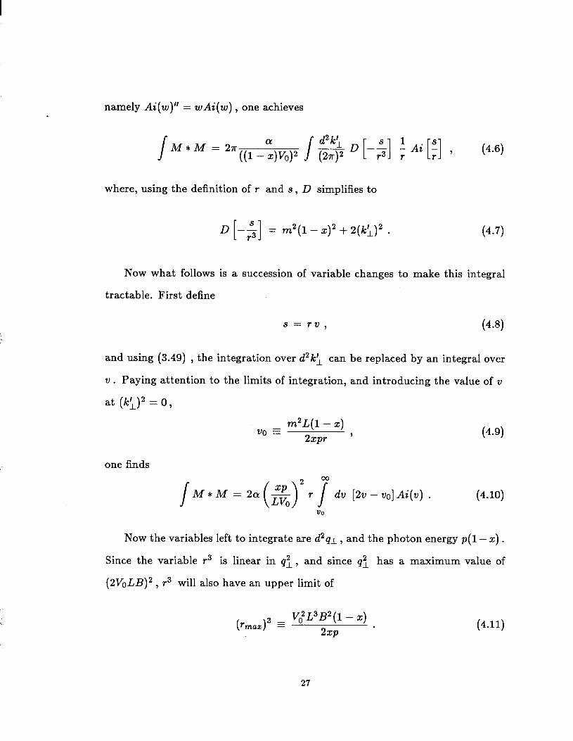
namely Ai( = wAi(w) , one achieves

J M*M = 27~ ((1 -$il)”

J 3 D [-;] ; Ai [;] , (4.6)

where, using the definition of r and s , D simplifies to

D -5 = m2(1 - x)~ + 2(k:)2 . [ 1 (4.7) Now what follows is a succession of variable changes to make this integral

tractable. First define

s = rv, (4.8)

and using (3.49) , the integration over d2kl can be replaced by an integral over

v . Paying attention to the limits of integration, and introducing the value of v

at (kl)2 = 0,

v. _ m2L(l - 4 2xpr ’ (4-g)

one finds

J M*M=2a (3g”r.T

dv [2v - vo] Ai . (4.10) VO

Now the variables left to integrate are d2ql, and the photon energy ~(1 - x) .

Since the variable r3 is linear in qt , and since q: has a maximum value of

(~VOLB)~, r3 will also have an upper limit of

(haz)3 - V,2LW(l- 2) 2xp *

(4.11)

27

If we write r = r mazt, where 0 < t < 1, then 00 = u/t, where u is the scaling

variable defined earlier, and

d2qI = 24~xp(V~LB)~ 3 t2dt , (4.12)

and the partial cross section for fixed photon energy fraction (1 - x) becomes

J?; J 7r2 M*M = J jdt3t3 Td+v-;]Ai(v), (4.13)

0 u/t

with

J = 12a(~pB)~ L3V,2B2 (1 - x) 1'3

2P 1 . X (4.14)

The integrations can be interchanged, the dt integration performed, and the

result is

J;? J cm

M*M= J dv J [ 3 U4

7r2 -v-u- 2 3 1 A+4 9 (4.15)

U

where the important scaling variable u is given by

( > 2

U3 =ce-I2 . X

(4.16)

28

Scaling Laws:

The differential cross section for beamstrahlung is achieved by dividing by the

normalization factors for the initial and final electron and photon wave functions,

[p3x(1-x)]; th f t e rat ional power spectrum by then multiplying by an extra factor

of (1 - Z) together with trivial numerical factors. The final result can be written

g = [ 2 x c R(u) 1 &classical ,

where the scaling spectrum function R(u) is defined as

cm R(u) = ; ?A2

J [ dv u4 iv-u- 2213

I A+) , U

(4.17)

(4.18)

The form factor described earlier is easily computed from the above results. Now

F(C) f 6 6 , classical

and since from the definition of u one has z = [l + u~/~/C]-’ , it follows that

1 03

F(C) = 2 dxxCR(u) = 3 s s

du u1/2

[1+ $3 R(u) * (4.20)

0 0

Explicitly, the form factor for the spin-zero case is

ccl 03 1 Ai . (4.21)

The normalization can be checked by taking the limit of large C and interchang-

29

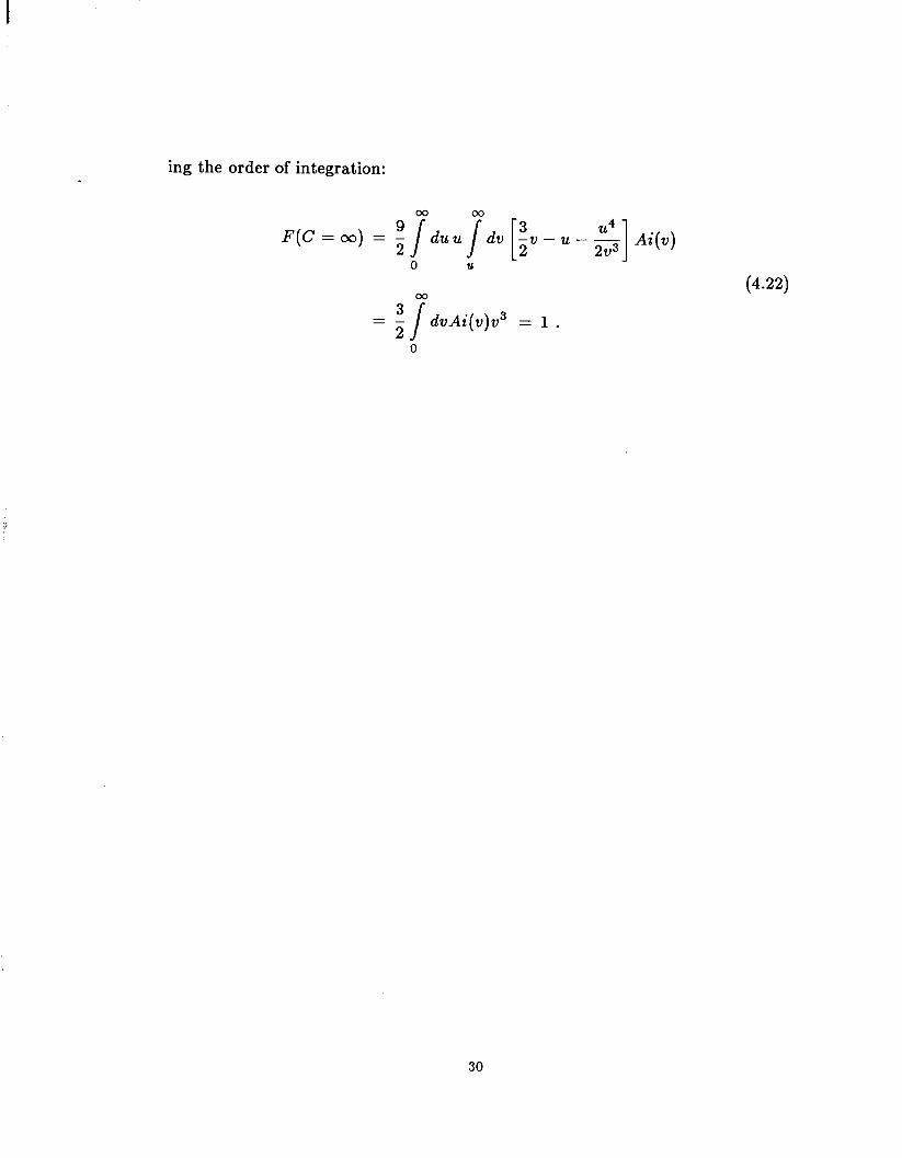
ing the order of integration:

F(C = 00) = 2 2/m d

0

uuj?dv [iv-u-$] Ai

U

(4.22)

3m =- 2 J

dvAi(v)v3 = I .

0

30

5. Dirac Electrons

The extension of our analysis to Dirac electrons is straightforward. The

general form of the matrix element for this case is

M = e c#J\-) (5-l)

where A is the photon field. It is convenient to use a chiral basis for the Dirac

spinors. The Hamiltonian and the Dirac equation take the form

H Q(r) = El@(r) ,

where in terms of the ordinary two-component Pauli matrices,

(5.2)

H= -iz+.$+v m

m +;ds7+V . >

The wave function will be written as

XP= +u ( > $1 ,

and the equation satisfied by the upper and lower components are

mh = (E - V - i-;;’ . V)$+

rn$l = (E-V+iZ’. ~)~u -

The second order equation satisfied by these components is

(5.3)

(5.4

(5.5)

m2qh = (E - V)2 + 7’ - i??. ez(t-) T,!I~ 1 m2$l =

[ (E -V)” + 7’ + i2 s e??(r) & , I

where ez(r) = -$V(r) .

31

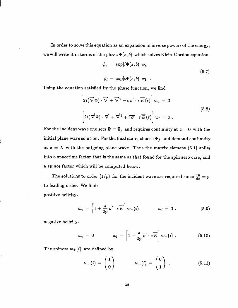
In order to solve this equation as an expansion in inverse powers of the energy,

we will write it in terms of the phase a(~, b) which solves Klein-Gordon equation:

A = q-@(O)] wu

P-7) $1 = exp[i@(z,b)] wl .

Using the equation satisfied by the phase function, we find

2i($Q). 3 + T2 - 3. eZ(r) wu = 0 1

For the incident wave one sets @ = @ i and requires continuity at z = 0 with the

initial plane wave solution. For the final state, choose @f and demand continuity

at z = L with the outgoing plane wave. Thus the matrix element (5.1) splits

into a spacetime factor that is the same as that found for the spin zero case, and

a spinor factor which will be computed below.

The solutions to order (l/p) for the incident wave are required since 2 = p

to leading order. We find:

positive helicity-

wu = [ l+ &Z.ed 1 w+(i) Wl = 0.

negative helicity-

wu = 0 wl = [ 1 - -&d .eZ w-(i) . I

The spinors w* (i) are defined by

1 0

w+(i) = 0 w-(i) = . 0 0 1

(5-g)

(5.10)

(5.11)

32

For the final state, the solutions to order (l/p!) are:

positive helicity-

w, = 1

negative helicity-

wu = 0

CL - “49 - ez 2Pf I w+(f) WI = 0. (5.12)

wl = l+ (L2ptz)T?-eX] w-(f) , (5.13)

The spinors w*(f) are helicity states along the final momentum, and to first

order they are

w+(f) = L ( > w-(f) = -!& 2Pf ( > 1'

(5.14)

The matrix element of the current is straightforward to evaluate from these

explicit solutions. Defining the transverse vectors V& = vZ f ivy, one finds that

there is no helicity flip amplitude, of course, and for:

positive helicity-

negative helicity-

1 - 2Pf

E-E+ E+E- -+-

P I Pf - (5.15)

E+E- c-E+ -+-

P I Pf - (5.16)

We now perform the sum over polarizations and the average over the initial

33

helicity states,

S(fermion) = i C (liTi+. ?I2 + (Id-. 212) . PO1

(5.17)

Taking into account the differing normalization conventions between fermions

and bosons, the fermion sum turns out to be a simple multiple of the boson sum:

1 + x2 S(fermion) = S(boson) 2a: .

6. Pulse Granularity and the Smoothness Assumption

In our previous discussion, we have assumed the distribution of charges in

the pulse to be smooth and uniform. In reality the pulse is a very long string of

length L = 7& as viewed in its rest frame. For the SLC, the parameters, (2.4) ,

indicate the pulse to be a dense string with radius B M 10m4 cm and interparticle

spacing L/N ra 2 x lo-‘cm << B . In this case it is natural to make a smooth

averaging of the charge distribution for the purpose of determining the trajectory

of the incident electron.

On the other hand, for the ‘super’ regime with parameters (2.10) , the pulse

is dilute with B = 5 x lo-‘cm and L/N ca 10m6 cm >> B , and it is thus necessary

to verify by direct calculation the validity of smoothing which was suggested by

the argument below (2.19) .

Our demonstration of the validity of this approximation follows from the form

of the electron wave function. The phase Cp in (3.8) contains integrals (3.9) and

(3.10) over the length of the pulse and hence effects of longitudinal variations

34

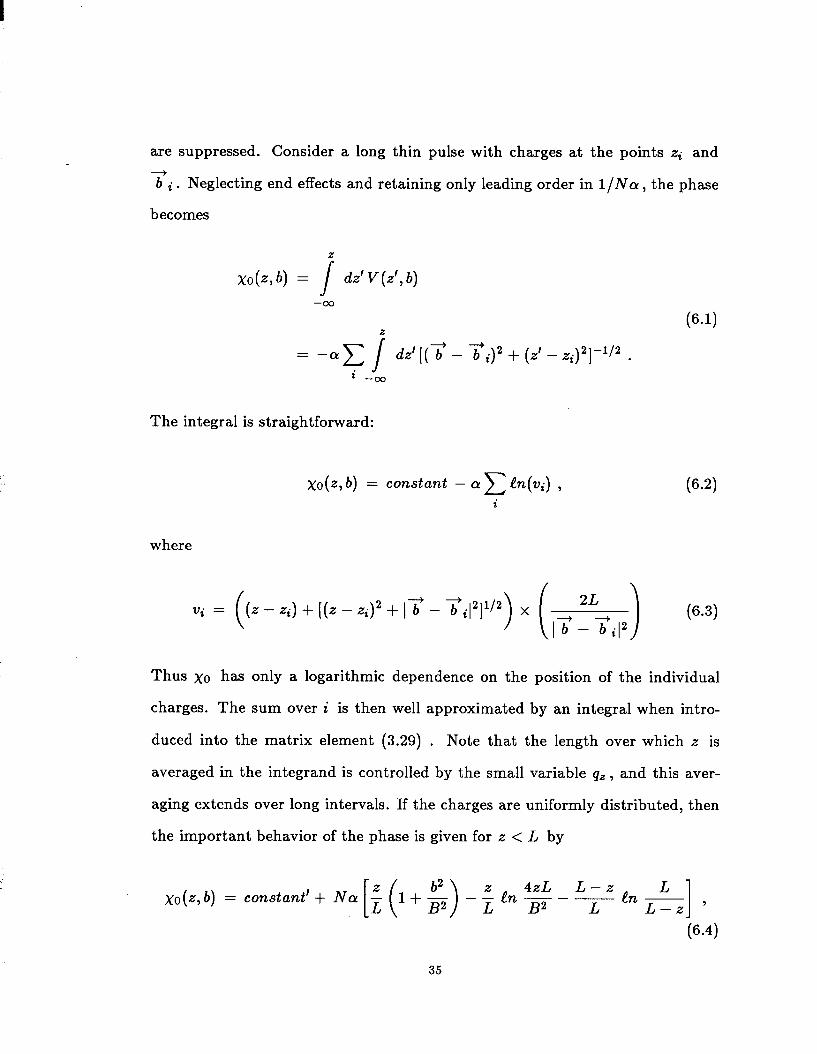
are suppressed. Consider a long thin pulse with charges at the points zi and

xi. Neglecting end effects and retaining only leading order in l/No, the phase

becomes

z XOW) = s dz’ V (z’, b)

-CC2 (64

= -ax j dz’[(%+ - Ti), + (z’ - zi)2~-W . i --co

The integral is straightforward:

Xo(z,q = constant - Eyx en(q) , i

(6.2)

where

vi = (z - Zi) + [(z - zJ2 + 17 - %+i12]1/2 (6*3)

Thus ~0 has only a logarithmic dependence on the position of the individual

charges. The sum over i is then well approximated by an integral when intro-

duced into the matrix element (3.29) . Note that the length over which z is

averaged in the integrand is controlled by the small variable qz , and this aver-

aging extends over long intervals. If the charges are uniformly distributed, then

the important behavior of the phase is given for z < L by

xo(z,b) = constant’+ Na[:(l+$)-g.h$--Th$---] ,

(6.4

35

while for z > L ,

xo(z, b) = constant’ + Ncr 4zL

-lngZ-- Z-L L ha -L-

Z-L I , (6.5)

where the logarithmic coulomb phase is extant. In particular, the relevant total

phase is of the form (see ref 20 )

03

xtt(b) = J

b2 dz’V(z’, b) = J&~(O) + N”ga .

-CO

Similarly, z

2Ncr -+ dz’ez - ’ = - LB2 zb .

(6.6)

P-7)

In addition, the current operators P(z, b) in (3.30) are unchanged. This com-

pletes our demonstration that smoothing is a good approximation, as was argued

qualitatively below (2.19) .

7. Review of Scaling Laws

At this point it may be useful to emphasize again results that are explicitly

contained in the above formulas. The fractional energy loss 6 for an electron

(of spin one-half) is a function of a (quantum) scaling variable that smoothly

extrapolates between the classical and the quantum results:

F(C) = 6 6 classical

1 [l ; U3/]2 + [l + l&4

u1i2R(u) , (7.1)

where R(u) is given by (4.18) . The power spectrum can also be written in a

36

scaling form:

1 d6 - = T(x) R(u) ,

Chatmica dx2

where T(x) = (x + l/x)/2 for electrons.

V-2)

Both of these are expressed in terms of the scaling variable u defined by

(7.3)

and

m3 me0 CT=-=- 2pVoJ3 47Y *

(74

Finally, the form factor and spectrum can be approximated by quite simple

analytic forms. By examining the limiting behavior of F(C) for large and small

C , and by evaluating analytically the integrals involved, one is lead to the form

F(C) = (

1+; [c- I)

-1

4/3 + 2 c-2/3 (1 + 0.2OC)43 , V-5)

where bl = 0.83... The asymptotic behavior of the Airy function at large argu-

ment, and the behavior of R(u) for small argument, suggest the approximate

form -1

R(u) = A~fi , P-6)

where A1 = 0.58... and a2 = 1.05... These approximate forms fit the exact

curves to within a few per cent and are graphed along with an exact numerical

integration in Figures la and 2. The fits can easily be improved.

37

8. Summary

We have studied the beamstrahlung process and derived formulas for the

photon spectrum and the average fractional energy loss. These results were

expressed in terms of scaling laws which should be convenient when comparing

different collider parameters.

Intermediate Collider:

Finally we apply these results to the parameters under study for a near term

collider at a center of mass energy of 650 Gev. One set of proposed parameters

is 1

N - 1 x lOlo 7 = 6.5 x lo5

(84 B - 7 x 10e6cm t?o = 6 x 10F2cm .

With these choices we find C fi: 1.5 and y x 4 x 10f2 . Note that this implies

6 classical = 1.3. Our measure of beam disruption is sizable, 6b/b - 2, requiring a

more careful treatment of the slicing technique than given in (2.24) . Neglecting

that important effect, we find that the fractional energy loss is also large, 6 =

0.38. Note that by doubling the beam length, C doubles, but the situation

is not changed much since the form factor increases by about 50%) leading to

6 = 0.29, a net 25% decrease. To decrease the fractional energy loss to 6 - 0.1,

it is necessary to increase the pulse length !?o by a factor of 10 over that given

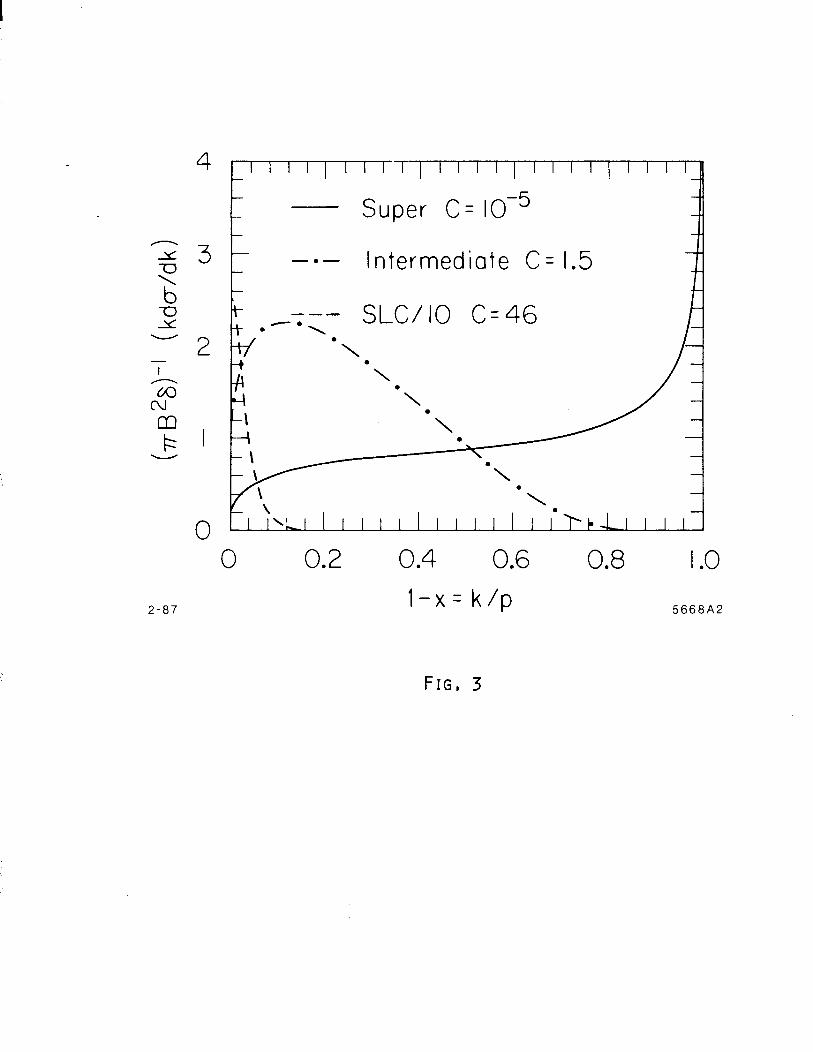
in (8.1) . In Figure 3 we have plotted the photon spectra (normalized to one) for

the SLC, the intermediate collider, and the super.

38

Regimes to Avoid:

The full luminosity is proportional to

Lum E Lump x f = N2

-f, 7TB2 (8.2)

where f is the number of pulses per second and Lump is equal to the luminosity

per pulse. Now consider the behavior of the fractional energy loss 6 as the

parameters are varied but with the luminosity per pulse, Lump, held fixed.

Other constraints will be ignored in this brief and incomplete discussion.

This means that the scaling variable y is fixed, since y = 2 &E%E’&. Thus

we can write

(8.3)

In order to choose a value of C that minimizes the fractional energy loss, note

that the ratio of F(C) to C vanishes for small C as C1i3, and vanishes for large

C as l/C. The worst choice for C is at the peak of the ratio which occurs at

C - 0.20 with a value - 0.275. This maximum, as shown in Figure la, is quite

wide; the ratio falls by a factor of 2 when C changes to 0.004 and 3.2. This

is the range of C to avoid in order to minimize 6 at a fixed luminosity. Thus

in order to minimize the fractional energy loss, one is forced into the classical

regime of large C or into the quantum regime of small C . Since C = m&/(47y) ,

this means either very long or very short pulses.

General Remarks:

Our results quantitatively confirm the arguments of Himel and Siegrist2 and

their adaptation of synchrotron radiation formulas to the collider situation. Their

final formula is remarkably accurate in the full quantum regime, C < 1.

39

Possible further extensions of this work include studies of more general pulse

charge distributions, studies of the effects of the curved trajectory on angular dis-

tributions in annihilation processes, especially for polarized beams, and a more

accurate discussion of the neglected end effects. It will be particularly important

to better understand the regime of large beam disruption. The case of electron-

proton collisions would be interesting to study since betatron-like oscillations

can be induced in the electron’s trajectory with minimal response by the proton

pulse. There are other applications of our technique which may prove interest-

ing and useful; among these are bremsstrahlung processes. involving relativistic

interactions with plasmas, astronomical phenomena, etc.

ACKNOWLEDGEMENTS

We wish to thank our experimental and accelerator colleagues for pointing out

the importance of this problem and for many enlightening conversations about

the physics involved. In particular, we wish to thank Tom Himel, Pisin Chen,

Wolfgang Panofsky, John Rees, and Burton Richter.

40

REFERENCES

1. For an overall review, see P. B. Wilson, SLAC-PUB-3985, May (1986).

2. T. Himel and J. Siegrist, SLAC-PUB-3572, February, 1985.

3. A.A. Sokolov and I.M. Ternov, ‘Synchrotron Radiation,’ Pergamon Press

(1968)) Berlin.

4. Schwinger source theory has been applied to the case of constant fields by

Pisin Chen and Robert Noble, SLAC-PUB-4050, August(1986) .

5. J. Schwinger, Proc. Nat. Acad. Sci. USA 40, 132 (19S4); Particles, Sources

and Fields, Vols. I and II, Addison-Wesley (1970,1973) Reading, Mass.

6. For a review of conversion processes in magnetic fields see Thomas Erber,

Rev. Mod. Phys. 98, 626 (1966).

7. An operator treatment for an inhomogeneous purely magnetic field has

been given by V.N. Ba:er and V.M. Katkov, Sov. Phys. JETP 28, 807

(1969), and Sov. Phys. JETP 26, 854 (1968).

8. H. A. Bethe and W. Heitler, Proc. Roy. Sot. Al46, 83 (1934).

9. H. A. Bethe and L. C. Maximon, Phys. Rev. 93, 768 (1954). H. Davies,H.

A. Bethe and L. C. Maximon, Phys. Rev. 99, 788 (1954).

10. James D. Bjorken, John B. Kogut, and Davison E. Soper, Phys. Rev. D9,

1382 (1971). S ee also John B. Kogut, and Davison E. Soper, Phys. Rev.

Dl, 2901 (1970).

11. Maurice Levy and Joseph Sucher, Phys. Rev. d86, 1656 (1969).

12. H. D. I. Abarbanel and C. I. Itzykson, Phys. Rev. Lett. Z?S, 53 (1969).

13. D. R. Harrington, Phys. Rev. DZ, 2512 (1970).

41

14. R. Blankenbecler and R. L. Sugar, Phys. Rev. D2, 3024 (1970).

15. This has been reduced by a factor of two from the formula given in 2 to

allow for the fact that the crossing speed of the collider pulses is 2c.

16. The scaling variable C is related to the ratio of the photon energy E to

its critical energy EC as defined in 2 , C = $g . c

17. In the case of a localized scatterer, relevant for the Bethe-Heitler case, one

finds that T(x) = $(z + l/x - 2/3).

18. This length plays the same role as the p/7, a parameter which is used

to describe an electron orbiting with radius p in the magnetic field of a

synchrotron.

19. Note that by (2.16) that the transverse momentum transfer will be - m

for path lengths 2 L/y.

20. This neglect of the coulomb phase is equivalent to the neglect of the radi-

ation that occurs before and after passage through the pulse.

21. This property is crucial since the phase itself is very large, of order Na,

which is - lo8 for our case, and few approximations can be tolerated.

22. See p. 447 of M. Abramowitz and I.A. Stegun, Handbook of Mathematical

Functions, U.S. Government Printing Office (1964), Washington, D.C.

42

FIGURE CAPTIONS

Figure la. The form factor plotted as a function of the scaling variable C, where

C = m2&,B/4yNa. The approximate form given in section 7 is plotted

as the dashed line. The ratio of the form factor to C is also plotted as the

dot-dash curve.

Figure lb. The same as Figure 1 except that the form factors are plotted on a loga-

rithmic scale.

Figure 2. The scaling form of the photon power spectrum is plotted as a function of

the variable u . The scaling spectrum is defined as

R(u) = $$z [T(x)Cbassical 1-l . The approximate form given in section 7 is

also plotted as the dashed curve. Recall that the fractional photon energy

is (l-x).

Figure 3. Three sample power spectra are plotted to illustrate the classical, transition,

and fully quantum regimes. They are normalized to unit area. The SLC

curve is divided by 10 for plotting purposes.

43

2 LL II

-

l-87

1.0

0.8

0.6

0.4

0.2

0

I I I I

- Fermion

--- A pprox .

-.- F(CVC

, .- I

-4 -2 0 2 4

LOG (C> 5668Al

FIG, 1~

F 0

G --I r 1

0

5 -2

-I 03 -3 - 9 -4 Lk

0 -

g -5

-I -6

2-87

FWC 1

\ \

\ \

\ \

\ \

\ \

\ \

F(C)

-4 -2 0 2 4 LOG (Cl 5668A4

- 3

- K

2-86

0.25

0.20

0.15

0. IO

0.05

0

Exact 4

Approx.

i

--

0 I 2 3

u = [C(l -x)/xl 2’3 4

5668A3

FIG, 2

b

0

2-87

I I 1 I

-.- Intermediate C= 1.5

Super C= 10B5

SLCAO C=46 t-i

0 02 . 04 . 06 . 08 . I .o

l-x= k/p 5668A2

FIG, 3