A Quantum N-Queens SolverValentin Torggler1, Philipp Aumann1, Helmut Ritsch1, and Wolfgang Lechner1,2

1Institute for Theoretical Physics, University of Innsbruck, A-6020 Innsbruck, Austria2Institute for Quantum Optics and Quantum Information of the Austrian Academy of Sciences, A-6020 Innsbruck, AustriaMay 29, 2019

The N-queens problem is to find the po-sition of N queens on an N by N chessboard such that no queens attack eachother. The excluded diagonals N-queensproblem is a variation where queens can-not be placed on some predefined fieldsalong diagonals. This variation is provenNP-complete and the parameter regimeto generate hard instances that are in-tractable with current classical algorithmsis known. We propose a special purposequantum simulator that implements theexcluded diagonals N-queens completionproblem using atoms in an optical lat-tice and cavity-mediated long-range inter-actions. Our implementation has no over-head from the embedding allowing to di-rectly probe for a possible quantum advan-tage in near term devices for optimizationproblems.

1 IntroductionQuantum technology with its current rapid ad-vances in number, quality and controllability ofquantum bits (qubits) is approaching a new erawith computational quantum advantage for nu-merical tasks in reach [1–11]. While buildinga universal gate-based quantum computer witherror-correction is a long-term goal, the require-ments on control and fidelity to perform algo-rithms with such a universal device that out-perform their classical counterparts are still elu-sive. Building special purpose quantum comput-ers with near-term technology and proving com-putational advantage compared to classical algo-rithms is thus a goal of the physics communityworld wide [12]. Quantum simulation with theaim to solve Hamiltonian systems may serve asa building block of such a special purpose quan-Wolfgang Lechner: wolfgang.lechner@uibk.ac.at

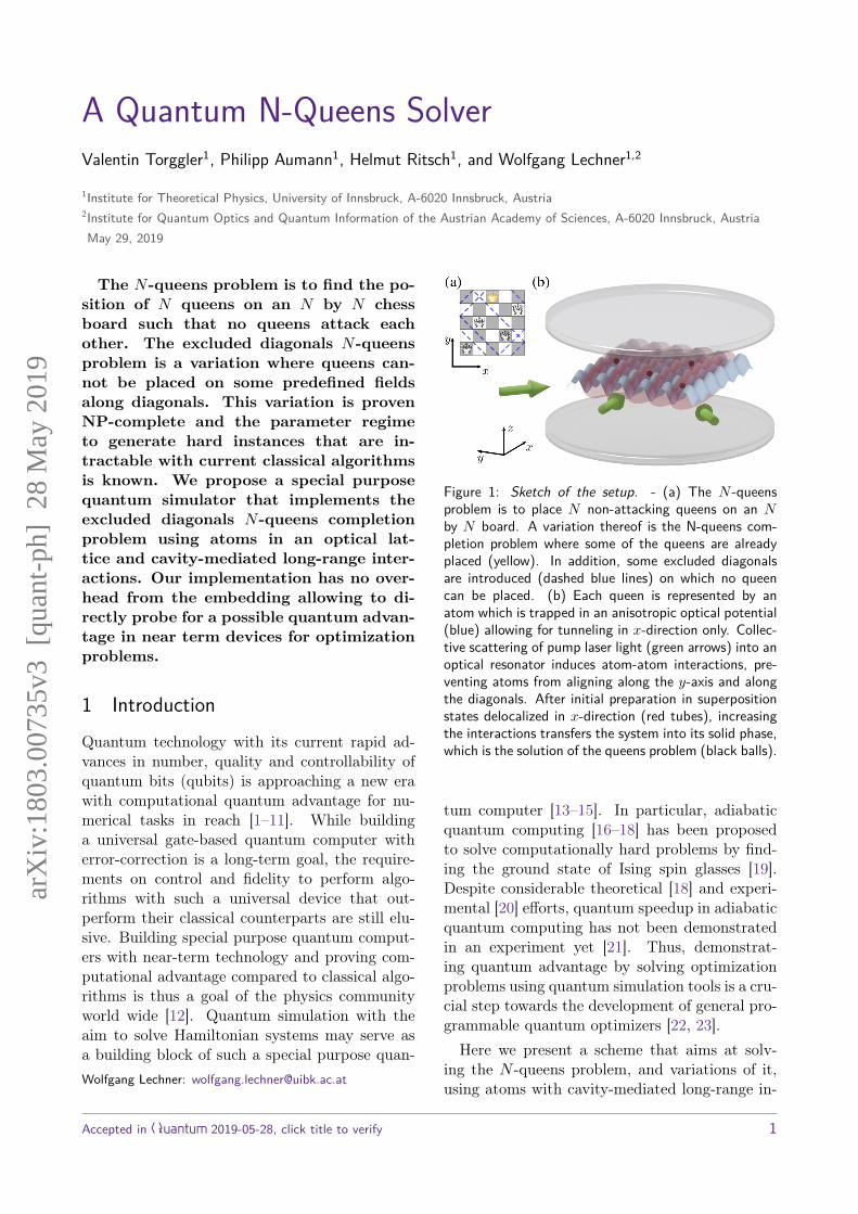
Figure 1: Sketch of the setup. - (a) The N -queensproblem is to place N non-attacking queens on an Nby N board. A variation thereof is the N-queens com-pletion problem where some of the queens are alreadyplaced (yellow). In addition, some excluded diagonalsare introduced (dashed blue lines) on which no queencan be placed. (b) Each queen is represented by anatom which is trapped in an anisotropic optical potential(blue) allowing for tunneling in x-direction only. Collec-tive scattering of pump laser light (green arrows) into anoptical resonator induces atom-atom interactions, pre-venting atoms from aligning along the y-axis and alongthe diagonals. After initial preparation in superpositionstates delocalized in x-direction (red tubes), increasingthe interactions transfers the system into its solid phase,which is the solution of the queens problem (black balls).

tum computer [13–15]. In particular, adiabaticquantum computing [16–18] has been proposedto solve computationally hard problems by find-ing the ground state of Ising spin glasses [19].Despite considerable theoretical [18] and experi-mental [20] efforts, quantum speedup in adiabaticquantum computing has not been demonstratedin an experiment yet [21]. Thus, demonstrat-ing quantum advantage by solving optimizationproblems using quantum simulation tools is a cru-cial step towards the development of general pro-grammable quantum optimizers [22, 23].

Here we present a scheme that aims at solv-ing the N -queens problem, and variations of it,using atoms with cavity-mediated long-range in-

Accepted in Quantum 2019-05-28, click title to verify 1

arX

iv:1

803.

0073

5v3

[qu

ant-

ph]

28

May

201

9

teractions [24–28]. We note that the N -queensproblem is not just of mathematical interest butalso has some applications in computer science[29]. In this work, variations of the problem areused as a testbed [30] to study a possible quan-tum advantage in solving classical combinatorialproblems in near term quantum experiments.

Our proposed setup consists of N ultracoldatoms in an optical lattice that represent thequeens on the chess board [31]. The non-attacking conditions are enforced by a combina-tion of restricted hopping [32] and interactionsbetween the atoms stemming from collective scat-tering of pump laser light into a multi-mode cav-ity [33–40] (see Fig. 1). For the excluded diag-onals variation of the N -queens problem, addi-tional repulsive optical potentials are introduced.The solution of the problem (or the ground stateof the many-body quantum system) is attainedvia a superfluid-to-solid transition. From themeasurement of photons that leave the cavity [41]it can be determined if a state is a solution to theN -queens problem. The position of the atomscan in addition be read out with single site re-solved measurement. The final solution is a clas-sical configuration and thus easy to verify. Weshow that a full quantum description of the dy-namics is required to find this solution.

Following Ref. [1], we identify a combinationof several unique features of the proposed modelthat makes it a viable candidate to test quan-tum advantage in near term devices. (a) Thecompletion and excluded diagonals problem isproven to be NP-complete and hard instances forthe excluded diagonals variant are known fromcomputer science literature [30], (b) the problemmaps naturally to the available toolbox of atomsin cavities and thus can be implemented with-out intermediate embedding and no qubit over-head, (c) the verification is computationally sim-ple and (d) the number of qubits required to solveproblems which are hard for classical computers(N > 21 for the solvers used in Ref. [30]) is avail-able in the lab.

Methods such as minor embedding [23, 42],LHZ [22, 43, 44] or nested embedding [45] alwayscause a qubit overhead. Here the intermediatestep of embedding the optimization problem inan Ising model is removed by implementing theinfinite-range interactions with cavity-mediatedforces tailored to the problem’s geometry in com-

bination with constrained tunneling [32]. Hencethere is no qubit overhead and the mode resourcesscale linearly with N . The required number ofqubits is reduced from several hundreds to below50, which is available in current experiments. Byimplementing our scheme with less than 50 atomsthe problem is already hard to tackle with currentclassical algorithms [30].

Light-mediated coupled tunneling gives rise tonon-local quantum fluctuations across the wholelattice in the intermediate stage of the transition[46, 47]. Their non-uniform signs stemming fromthe relative phases of the cavity fields from siteto site indicate that the system’s Hamiltonianis non-stoquastic and can thus not be efficientlysimulated with path integral Monte Carlo meth-ods on a classical computer [48]. The questionof a quantum speed-up is thus open unless a lo-cal transformation to a stoquastic Hamiltonian isfound [49, 50].

In our model implementation the non-localqubit interactions are mediated via the fieldmodes of an optical resonator, which will attainnon-classical atom-field superposition states dur-ing the parameter sweep. This appears to bean essential asset of the system as we find thatthe ground-state is reached only with a very lowprobability, when the full quantum dynamics ofthe fields is replaced by a classical mean-field ap-proximation.

As a final feature let us point out here that theverification of a solution is computationally triv-ial as the final state is classical and no quantumtomography is needed. In principle the conver-gence to a solution can be simply deduced fromthe cavity outputs at the end of the sweep. Withthis, the proposed setup may serve as a plat-form to demonstrate combinatorial quantum ad-vantage in near-term experiments.

This work is organized as follows: In Sec. 2we introduce a quantum model based on coupledquantum harmonic oscillators simulating the Nqueens problem. A proposed physical implemen-tation using ultracold atoms in optical latticesand light-mediated atom-atom interaction is de-scribed in Sec. 3. In Sec. 4 we present a numericalcomparison between model and implementationincluding photon loss. Finally we discuss in Sec.5 how light leaking out of the cavity can be usedfor read-out and we conclude in Sec. 6.

Accepted in Quantum 2019-05-28, click title to verify 2

2 Quantum simulation of the N -queens problemFollowing the idea of adiabatic quantum compu-tation [16–18], we construct a classical problemHamiltonian Hpr such that its ground state corre-sponds to the solutions of the N -queens problem.In order to find this ground state, the system isevolved with the time-dependent Hamiltonian

H(t) = Hkin + t

τHpr (1)

from t = 0 to t = τ . Initially at t = 0,the system is prepared in the ground state ofH(0) = Hkin. During the time evolution, thesecond term is slowly switched on. If this pa-rameter sweep is slow enough, the system staysin the instantaneous ground state and finally as-sumes the ground state of H(τ) at t = τ . If thelowest energy gap of Hpr is much larger than theone of Hkin, this state is close to the ground stateof Hpr and thus the solution of the optimizationproblem.

In the following we construct the problemHamiltonian Hpr and the driver HamiltonianHkin. The system is modeled as a 2D Bose-Hubbard model with annihilation (creation) op-erators bij (b†ij) on the sites (i, j). A positionof a queen is represented by the position of anatom in an optical lattice with the total numberof atoms being fixed to N . The non-attackingcondition between queens, which amounts to in-teractions between two sites (i, j) and (k, l), is im-plemented with four constraints: There can notbe two queens on the same line along (i) the x-direction j = l, (ii) the y-direction i = k, thediagonals (iii) i+ j = k+ l and (iv) i− j = k− l.

Condition (i) is implemented by using an initialstate with one atom in each horizontal line at yjand restricting the atomic movement to the x-direction [see Fig. 1(b)]. Thereby we use the apriori knowledge that a solution has one queen ina row, which reduces the accessible configurationspace size from

(N2

N

)toNN configurations. In this

vein the restricted tunneling Hamiltonian [32] isgiven by

Hkin = −JN∑

i,j=1Bij , (2)

where J is the tunneling amplitude and Bij =b†i,jbi+1,j + b†i+1,jbi,j with BNj = 0 are the tunnel-ing operators.

Constraints (ii), (iii) and (iv) are enforcedby infinite range interactions between the atomswith

HQ = UQ

N∑ijkl=1

Aijkl nijnkl, (3)

where ni,j = b†i,jbi,j and UQ > 0. The interactionmatrix is

Aijkl =

3 if (i, j) = (k, l)1 if i = k ∨ i+ j = k + l ∨ i− j = k − l0 otherwise,

(4)where in the first case all three constraints arebroken.

In order to implement variations of the N -queens problem, we need to exclude diagonals (forthe excluded diagonals problem) and pin certainqueens (for the completion problem). These addi-tional conditions are implemented by local energyoffsets of the desired lattice sites

Hpot = UD

N∑i,j=1

Dij nij − UT

N∑i,j=1

Tij nij . (5)

For UD > 0 the first term renders occupationsof sites on chosen diagonals energetically unfa-vorable. Each diagonal (in + and − direction)has an index summarized in the sets D+ and D−,respectively, and the coefficients are

Dij =

2 if i+ j − 1 ∈ D+ ∧ i− j +N ∈ D−1 if i+ j − 1 ∈ D+ ∨ i− j +N ∈ D−0 otherwise.

(6)For UT > 0, the second term favors occupationsof certain sites. The sites where queens should bepinned to are pooled in the set T and thereforethe coefficients are given by

Tij =

1 if (i, j) ∈ T0 otherwise.

(7)

The problem Hamiltonian of the N -queens prob-lem with excluded diagonals is then

Hpr = HQ +Hpot. (8)

Note that due to the initial condition atoms nevermeet and sites are occupied by zero or one atomonly. Hence the system can be effectively de-scribed by spin operators [31, 40], also withoutlarge contact interactions.

Accepted in Quantum 2019-05-28, click title to verify 3

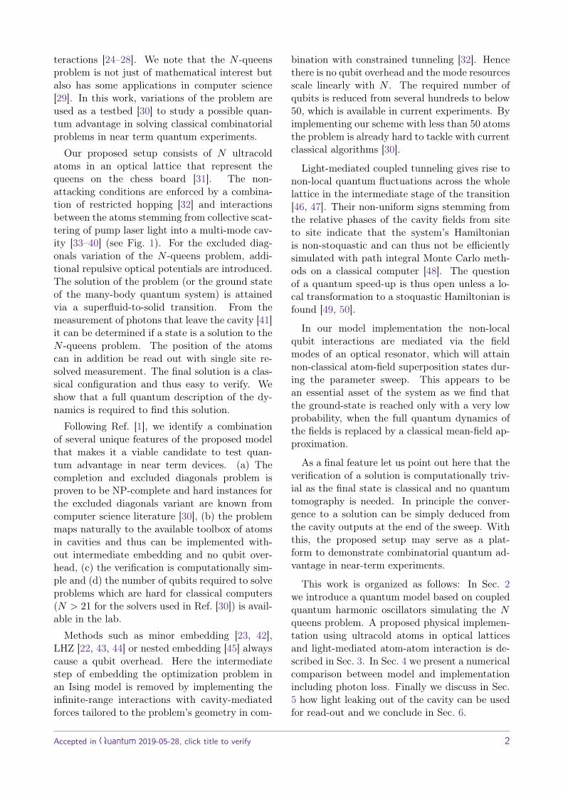
Figure 2: Time evolution of site occupations. - Eachsubplot shows a snapshot of the site occupations 〈nij〉for the parameter sweep in Eq. (1) and a sweep timeJτ/~ = 49. This is the instance shown in Fig. 1a, wherethe excluded diagonals are indexed by D+ = 2, 3, 6, 9and D− = 1, 2, 8, 9 and one queen is pinned at site(3, 5), i.e. T = (3, 5) (see text). The final values ofthe sweep are UQ = J , UD = 5J , UT = 2J while J iskept constant. Since the sweep time is large enough, thestate of the system adiabatically converges to the uniquesolution of the problem, which can be easily verified.

Let us illustrate the parameter sweep in Eq.(1) for a specific example instance with N = 5queens (see Fig. 1). The excluded diagonals cho-sen here restrict the ground state manifold totwo solutions, and by biasing site (3, 5) one ofthese solutions is singled out. The time evolu-tion of the site occupations 〈nij〉 from numericallysolving the time-dependent Schrödinger equationis shown in Fig. 2. Initially, the atoms arespread out in x-direction since the ground stateof H(0) = Hkin is a superposition of excitationsalong each tube. After evolving for a sufficientlylarge time Jτ/~ = 49, the system is in the groundstate of Hpr and thus assumed the solution of theoptimization problem.

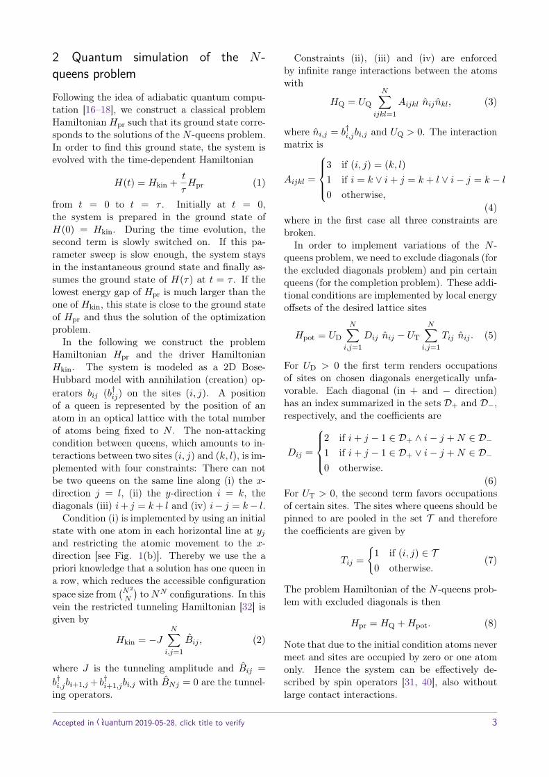
The energy spectrum of the given instance isshown in Fig. 3(a). The minimal gap betweenground state (orange) and first excited state(green) determines the minimum sweep time τto remain in the ground state according to theLandau-Zener formula. At the end of the sweep,the ground state closely resembles the solution tothe excluded diagonals problem shown in Fig. 1.

The Hilbert space for the atomic state corre-sponding to the configuration space mentionedabove grows exponentially as NN and thus, asusual for quantum systems, the computationalcosts get large for rather small systems. Simula-tions with significantly larger systems are hencenot easily tractable.

Figure 3: Energy spectrum. - Eigenvalue spectrum ofH(t) for (a) the model Hamiltonian [Eq. (1)] and (b)the Hamiltonian created by the field-atom interactions[Eq. (10)] for the instance described in Fig. 2. The or-ange and green lines show ground state and first excitedstate, respectively. The blue lines depict higher energyeigenstates. The low energy sector, and especially theminimal gap, are qualitatively similar.

3 Implementation

Here we propose a specific and at least concep-tionally simple and straightforward physical im-plementation of Eq. (1), where the N queens aredirectly represented by N ultracold atoms in anNxN two-dimensional optical lattice. Assumingtight binding conditions the atoms are confined tothe lowest band of the lattice. They can coher-ently tunnel between sites [51] and interact viacollective light scattering within an optical res-onator. To implement the required queens inter-actions via light scattering we make use of a setof optical field modes in a multi-mode standing-wave resonator [see Fig. 1(b)]. It was shown be-fore that this configuration in principle allows toimplement arbitrary site to site interactions [40]if a sufficient number of modes is used.

To reduce the necessary Hilbert space withoutloss of generality, it is sufficient to enable tun-neling only along one dimension (x), e.g. therows of the lattice and increase the lattice depthin the column (y) direction. This confines theatoms (queens) to move only along tubes in thex-direction forming a parallel array of N 1D opti-cal lattices as routinely used to study 1D physicswith cold atoms [52].

Luckily, for the special case of the infinite rangequeens interactions, one can find a strikingly sim-ple and intuitive example configuration requiringonly few field modes for each of the three re-maining queens interaction directions. For thiswe consider the optical lattice to be placed in thecenter symmetry plane of the optical resonator,where one has a common anti-node of all sym-

Accepted in Quantum 2019-05-28, click title to verify 4

metric eigenmodes. The trapped atoms are thenilluminated by running plane wave laser beamsfrom three different directions within the latticeplane with frequencies matched to different lon-gitudinal cavity modes.

Depending on the size of the problem we needto add more laser frequencies in each directionto avoid a periodic recurrence of the interac-tion within the lattice. Note that all frequenciescan be easily derived and simultaneously stabi-lized from a single frequency comb with a spac-ing matched to the cavity length. Since all lightfrequencies are well separated compared to thecavity line width, each is scattered into a dis-tinct cavity mode and as the cavity modes arenot directly coupled no relative phase stabilityis needed [40]. The resulting position-dependentcollective scattering into the cavity then intro-duces the desired infinite-range interactions be-tween the atoms. Choosing certain frequenciesand varying their relative pump strengths al-lows for tailoring these interactions to simulatethe three non-attacking conditions in the queensproblem discussed in the previous section. Addi-tional light sheets and local optical tweezers canbe used to make certain diagonals energeticallyunfavorable (for the excluded diagonal problem)or pin certain queens. Alternatively pinning canbe achieved by selective cavity mode injection.

In the first part (Sec. 3.1) we will now intro-duce a Bose-Hubbard-type Hamiltonian for thetrapped atoms interacting via collective scatter-ing for general illumination fields in more detail.For this we first consider the full system of cou-pled atoms and cavity modes and later adiabati-cally eliminate the cavity fields to obtain effectivelight-mediated atom-atom interactions.

In the second part (Sec. 3.2) we discuss how toimplement the non-attacking conditions of theN -queens problem with such light-mediated atom-atom interactions. Specifically, we consider thelimit of a deep optical lattice leading to sim-ple analytical expressions. These formulas allowus to find a specific pump configuration of wavenumbers and pump strengths leading to the idealqueens interaction Hamiltonian in Eq. (3). Asa deep lattice depth slows down atomic tunnel-ing it requires long annealing times. Luckily, itturns out that the pump configuration derived fora deep lattice still gives the same ground statefor moderate lattice depth with faster tunneling.

We show this by numerical simulations in Sec. 4.While the details of the interaction are altered itstill sufficiently well approximates the N -queensinteraction.

3.1 Tight-binding model for atoms interactingvia light

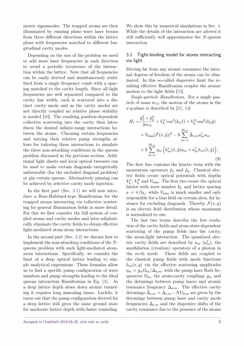
Driving far from any atomic resonance the inter-nal degrees of freedom of the atoms can be elim-inated. In this so-called dispersive limit the re-sulting effective Hamiltonian couples the atomicmotion to the light fields [53].Single-particle Hamiltonian. For a single par-

ticle of mass mA, the motion of the atoms in thex-y-plane is described by [25, 54]

H1 =p2x + p2

y

2mA+ V x

L cos2(kLx) + V yL cos2(kLy)

+ Vbias|F(x, y)|2 − ~Mtot∑m=1

∆c,ma†mam

+ ~Mtot∑m=1

ηm(h∗m(x, y)am + a†mhm(x, y)

).

(9)The first line contains the kinetic term with themomentum operators px and py. Classical elec-tric fields create optical potentials with depthsV x

L , V yL and Vbias. The first two create the optical

lattice with wave number kL and lattice spacinga = π/kL, while Vbias is much smaller and onlyresponsible for a bias field on certain sites, for in-stance for excluding diagonals. Thereby F(x, y)is an electric field distribution whose maximumis normalized to one.

The last two terms describe the free evolu-tion of the cavity fields and atom-state-dependentscattering of the pump fields into the cavity,the atom-light interaction. The quantized elec-tric cavity fields are described by am (a†m), theannihilation (creation) operators of a photon inthe m-th mode. These fields are coupled tothe classical pump fields with mode functionshm(x, y) via the effective scattering amplitudesηm = gmΩm/∆a,m, with the pump laser Rabi fre-quencies Ωm, the atom-cavity couplings gm andthe detunings between pump lasers and atomicresonance frequency ∆a,m. The effective cavitydetunings ∆c,m = ∆c,m−NU0,m are given by thedetunings between pump laser and cavity modefrequencies ∆c,m and the dispersive shifts of thecavity resonance due to the presence of the atoms

Accepted in Quantum 2019-05-28, click title to verify 5

in the cavity NU0,m [24].Note that, for example by placing the opti-

cal lattice (x-y-plane) in a common anti-node ofthe standing wave cavity modes and exciting onlyTEM00 modes, the atom-cavity coupling is uni-form in space in our model. Thus the only spatialdependence in the cavity term is due to the pumpfields.Generalized Bose-Hubbard Hamiltonian. The

atom-atom interactions are taken into accountby introducing bosonic field operators Ψ(x) withH =

∫d2xΨ†(x)H1Ψ(x) [25, 55]. Note that we

do not include contact interactions since atomsnever meet due to the initial condition we willuse. We assume that the optical lattice withdepths V x

L and V yL is so deep, that the atoms are

tightly bound at the potential minima and onlythe lowest vibrational state (Bloch band) is occu-pied. Moreover, the optical potential created bybias and cavity fields is comparably small, suchthat the form of the Bloch wave functions only de-pends on the optical lattice [54]. In this limit wecan expand the bosonic field operators in a local-ized Wannier basis Ψ(x) =

∑i,j w2D(x − xij)bij

with the lowest-band Wannier functions w2D(x)coming from Bloch wave functions of the lattice[56]. We split the resulting Hamiltonian in threeterms

H = Hkin +Hcav +Hpot, (10)which will be explained in the following.

As in the standard Bose-Hubbard model, oneobtains a tunneling term Hkin as in Eq. (2). Tun-neling in y-direction is frozen out by ensuringV y

L V xL . The other terms Hcav and Hpot

originate from the weak cavity-pump interferencefields and the bias fields introduced above andshould resemble Hpr [Eq. (8)]. In order to realizethe sweep Eq. (1), the relative strength of theseterms and the kinetic term has to be tuned, e.g.by ramping up the pump laser and bias field in-tensity (make Hcav and Hpot larger) or the latticedepth (make Hkin smaller).

The cavity-related terms in Eq. (9) give rise to

Hcav =− ~∑m

∆c,ma†mam

+ ~∑m

Nηm(Θ†mam + a†mΘm

) (11)

with the order operator of cavity mode m

Θm = 1N

N∑i,j=1

(vijmnij + uijmBij

). (12)

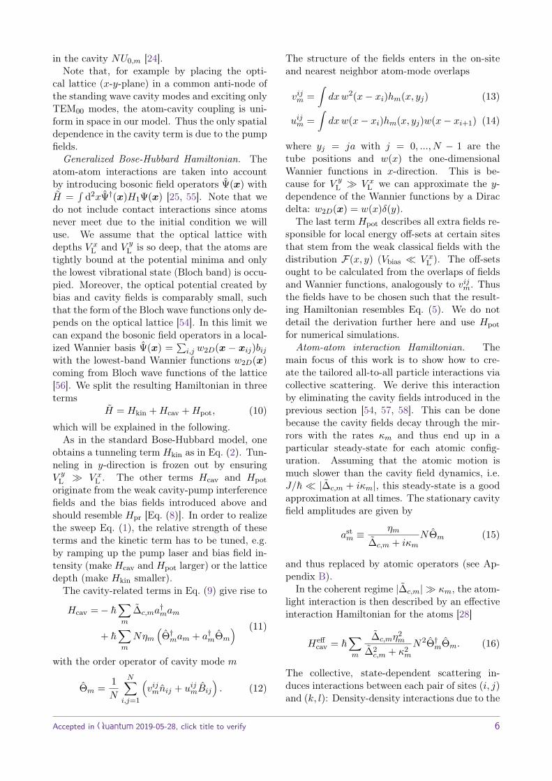
The structure of the fields enters in the on-siteand nearest neighbor atom-mode overlaps

vijm =∫dxw2(x− xi)hm(x, yj) (13)

uijm =∫dxw(x− xi)hm(x, yj)w(x− xi+1) (14)

where yj = ja with j = 0, ..., N − 1 are thetube positions and w(x) the one-dimensionalWannier functions in x-direction. This is be-cause for V y

L V xL we can approximate the y-

dependence of the Wannier functions by a Diracdelta: w2D(x) = w(x)δ(y).

The last term Hpot describes all extra fields re-sponsible for local energy off-sets at certain sitesthat stem from the weak classical fields with thedistribution F(x, y) (Vbias V x

L ). The off-setsought to be calculated from the overlaps of fieldsand Wannier functions, analogously to vijm. Thusthe fields have to be chosen such that the result-ing Hamiltonian resembles Eq. (5). We do notdetail the derivation further here and use Hpotfor numerical simulations.Atom-atom interaction Hamiltonian. The

main focus of this work is to show how to cre-ate the tailored all-to-all particle interactions viacollective scattering. We derive this interactionby eliminating the cavity fields introduced in theprevious section [54, 57, 58]. This can be donebecause the cavity fields decay through the mir-rors with the rates κm and thus end up in aparticular steady-state for each atomic config-uration. Assuming that the atomic motion ismuch slower than the cavity field dynamics, i.e.J/~ |∆c,m + iκm|, this steady-state is a goodapproximation at all times. The stationary cavityfield amplitudes are given by

astm ≡

ηm

∆c,m + iκmNΘm (15)

and thus replaced by atomic operators (see Ap-pendix B).

In the coherent regime |∆c,m| κm, the atom-light interaction is then described by an effectiveinteraction Hamiltonian for the atoms [28]

Heffcav = ~

∑m

∆c,mη2m

∆2c,m + κ2

m

N2Θ†mΘm. (16)

The collective, state-dependent scattering in-duces interactions between each pair of sites (i, j)and (k, l): Density-density interactions due to the

Accepted in Quantum 2019-05-28, click title to verify 6

terms containing nijnkl and a modified tunnel-ing amplitude due an occupation or a tunnelingevent somewhere else in the lattice due to nijBkl,Bijnkl and BijBkl. While the density-densityinteractions constitute the problem Hamiltonian[see Eq. (3)], the latter cavity-induced tunnelingterms lead to non-local fluctuations which mighthelp to speed up the annealing process [46].

Since the Wannier functions are localized atthe lattice sites, the on-site overlaps vijm tend tobe much larger than the nearest-neighbor over-laps uijm. Thus density-density interactions areexpected to be the dominant contribution toHeff

cav. As intuitively expected, the atoms local-ize stronger for deeper lattices, where analyti-cal expressions for the overlaps can be obtainedwithin a harmonic approximation of the poten-tial wells leading to Gaussian Wannier functionswith a width ∝ (V x

L )−1/4. Apart from a correc-tion factor due to this width, the on-site over-laps are given by the pump fields at the lat-tice sites. The nearest-neighbor overlaps corre-spond to the pump fields in between the latticesites, but are exponentially suppressed (see Ap-pendix C). Consequently, in the deep lattice limit(large V x

L ) when the width tends to zero we getvijm = hm(xi, yj) and uijm = 0 [28], and an interac-tion Hamiltonian [from Eq. (16)]

Hdlcav = ~

∑m

∆c,mη2m

∆2c,m + κ2

m

×∑ijkl

h∗m(xi, yj)hm(xk, yl)nijnkl,

(17)which only depends on density operators, andhence does not include cavity induced-tunneling.

3.2 N -queens interactionIn this section we aim to find pump fields hm(x, y)such that the interaction Hamiltonian in thedeep lattice limit Eq. (17) corresponds to the de-sired queens Hamiltonian HQ [Eq. (3)] containingthe non-attacking conditions. Using these pumpfields we later show numerically in Sec. 4, that theatom-atom interaction for realistic lattice depths[Eq. (16)], although slightly altered, still well re-sembles the queens interaction.

We consider three sets of M parallel runningwave laser beams with different propagation di-rections, each of which could be created by a fre-quency comb. The three directions are perpen-

dicular to the lines along which queens shouldnot align, that is along the x-direction and alongthe diagonals. We denote the corresponding wavevectors with kxm = (k0

m, 0)T , k+m = (k0

m, k0m)T and

k−m = (k0m,−k0

m)T , respectively, with the wavenumbers k0

m. Therefore the pump fields are givenby

hm(x, y) = eikmx, (18)

where x = (x, y)T is the position vector and kmis a wave vector in any of the three directions.

With running wave pump fields, Eq. (17) canbe written as

Hdlcav = UQ

∑ijkl

Aijklnijnkl. (19)

This formally corresponds to HQ [Eq. (3)], wherethe quantities now have a physical meaning: Theinteraction matrix is given by

Aijkl =∑m

fm cos(km(xij − xkl)) (20)

with lattice site connection vectors xij −xkl and

fmUQ = ~∆c,mη

2m

∆2c,m + κ2

m

(21)

with∑M−1m=0 fm = 1. The dimensionless param-

eters fm capture the relative strengths of themodes, determining the shape of the interaction.They have to be chosen such that A approximatesA [Eq. (4)]. The overall strength of the interac-tion term is captured by the energy UQ, whichcan be easily tuned by the cavity detunings orthe pump intensities to implement the parametersweep in Eq. (1). For the following discussion wedefine an interaction function

A(r) =∑m

fm cos(kmr) (22)

which returns the interaction matrix when eval-uated at lattice site connection vectors Aijkl =A(xij − xkl).

We note that one set of parallel kµm (µ ∈x,+,−) creates an interaction A which is con-stant and infinite range (only limited by the laserbeam waist) in the direction perpendicular to thepropagation direction r ⊥ kµm. Along the prop-agation direction r ‖ kµm instead, the interactionis shaped according to the sum of cosines, andcan be modified by the choice of wave numberskµm = |kµm| and their relative strengths fm.

Accepted in Quantum 2019-05-28, click title to verify 7

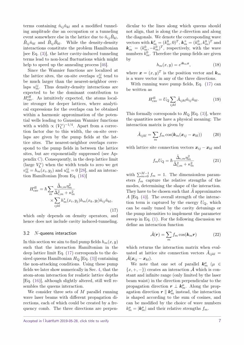
In the following we will use the example wavenumbers

k0m = kL

(1 + 2m+ 1

2M

)(23)

with m = 0, ...,M − 1 and uniform fm = 1/M .Taking into account kxm only, the interactionalong the x-direction r ‖ kxm at lattice site dis-tances rj = jπ/kL = ja has the values

A(rj) =

(−1)l for j = 2Ml, l ∈ Z0 otherwise,

(24)

as shown in Appendix D. If we guarantee that−2M < j < 2M this results in an interac-tion which is zero everywhere apart from j = 0,i.e. at zero distance. So for repulsive interac-tions (UQ > 0 and thus ∆c,m > 0), the wavevectors kxm create the non-attacking interactionalong the y-direction (Aijkl = 1 if i = k and 0otherwise) as long as N ≤ 2M . This is illus-trated in Fig. 4(a) for M = N = 5. Analo-gously, k±m cause the non-attacking interactionsalong the diagonals. In a square lattice the di-agonals have the distance rj/

√2, which is com-

pensated by k±m = |k±m| =√

2k0m. Since there

are 2N − 1 diagonals, one has to make sure that2N − 1 ≤ 2M . Upon combining all wave vectorsfrom three directions we finally obtain the fullqueens interaction, as shown in Fig. 4(b), whichis realized with Mtot = 3M = 3N frequencies inour example.

Note that there are several combinations ofwave numbers and mode strengths which, at leastapproximately, create the desired line-shaped in-teractions perpendicular to the light propagationdirection. For this it is insightful to reformulatethe interaction as a Fourier transform. To dealwith continuous functions, we define an envelopef(k) with f(km) = fm, which is sampled at thewave numbers n∆k with n ∈ Z containing allkµm. Considering one illumination direction forsimplicity, the interaction [Eq. (22)] along r ‖ kµmwith r = |r| can be written as

A(r) = Re[√

2πFf(k)

∞∑n=−∞

δ(k − n∆k)

(r)]

=∞∑

l=−∞Re[√

2πFf(r − l 2π

∆k

)],

(25)where Ff(r) =

∫∞−∞ dkf(k)eikr/

√2π is the

Fourier transform of f(k) and δ(x) is a Dirac

Figure 4: Energy penalty created by one atom. - Thesedensity plots show the energy penalty A(x − xa) foran atom at position x = (x, y)T created by an atomat position xa = (a, a)T (red dot) for N = M = 5[see Eq. (22)]. The dots indicate lattice site posi-tions and the solid (dashed) contour lines indicate whereA(x−xa) = 0 (A(x−xa) = 1) is fulfilled. (a) Pumpingalong the x-axis with the wave vectors kx

m = (k0m, 0)T

with k0m/kL = 1.1, 1.3, 1.5, 1.7, 1.9 [according to Eq.

(23)] creates interactions along y. (b) Additionally in-cluding diagonal pump lasers k+

m = (k0m, k

0m)T and

k−m = (k0

m,−k0m)T implements the full queens inter-

action along diagonals and vertical lines [Eq. (3)].

delta at x = 0. See Appendix D for a detailedderivation.

The last line allows for a simple interpretation:The interaction consists of peaks repeating witha spatial period R = 2π/∆k. Each of these peakshas the shape of the real part of the Fourier trans-form of the envelope function f(k) with a widthcorresponding to the inverse of the mode band-width σ ∼ 2π/∆kBW.

For the (approximate) non-attacking condition(A(ja) ≈ 1 for j = 0 and |A(ja)| 1 other-wise) there are two conditions. Firstly, at mostone peak should be within the region of theatoms. Thus the period has to be larger thanthe (diagonal) size of the optical lattice R ≥ Na(R ≥

√2Na). Secondly, the width of one peak

has to be smaller than the lattice spacing σ . a.Combining these conditions to R & Nσ, we seethat the minimum number of modes per directionM scales linearly with N

M ≈ ∆kBW/∆k & N. (26)

Therefore, with only ∼ N modes this quite gener-ically allows for creating an interaction along linesperpendicular to the light propagation. Notehowever, that the second condition also impliesthat the spatial frequency spread has to be at

Accepted in Quantum 2019-05-28, click title to verify 8

least on the order of the lattice wave number∆kBW & kL.

4 Numerical justification of assump-tions

We compare the ideal model Hamiltonian de-scribed in Sec. 2 [Eq. (1)] to the physically mo-tivated tight-binding Hamiltonian for finite lat-tice depths introduced in Sec. 3 [Eq. (10)]. Asfor the ideal model in Fig. 2, we consider thetime evolution during a slow linear sweep of UQ,UT and UD by numerically integrating the time-dependent Schrödinger equation. Physically, thissweep can be realized by ramping up the pumpand the bias field intensities. Moreover, we showthat evolving the system using a classical approx-imation for the cavity mode fields does not resultin a solution to the N -queens problem, and ad-dress the effect of dephasing by photon loss withopen system simulations.

In the following we use a realistic lattice depthof V x

L = 10ER with the recoil energy ER =~2k2

L/(2mA). For example, for rubidium 87Rband λL = 785.3 nm it is ER/~ = 23.4 kHz [26].The chosen lattice depth leads to a tunneling am-plitude J ≈ 0.02ER, which can be obtained fromthe band structure of the lattice. We consider ourcavity model in Eq. (10) for N = 5. The pumpmodes are as in Sec. 3.2 and Fig. 4. While inthe limit of a deep lattice this would result in theideal model interactions, here they depend on theoverlaps between Wannier functions and pumpmodes [Eq. (13)] and are thus altered. In thefollowing the overlaps are calculated with Wan-nier functions which where numerically obtainedfrom the band structure of the lattice. It turnsout, that the deviation from the ideal overlapsdoes not qualitatively change the interaction forthe realistic parameters used.

4.1 Coherent dynamics

The energy spectrum of the Hamiltonian for fi-nite lattice depths in Eq. (16) is shown in Fig.3(b) and is qualitatively of the same form as forthe ideal model in Fig. 3(a). In comparison theeigenvalue gaps tend to be smaller at the endof the sweep. This is because the on-site atom-mode overlaps decrease for shallower lattices andless localized atoms due to a smoothing of the

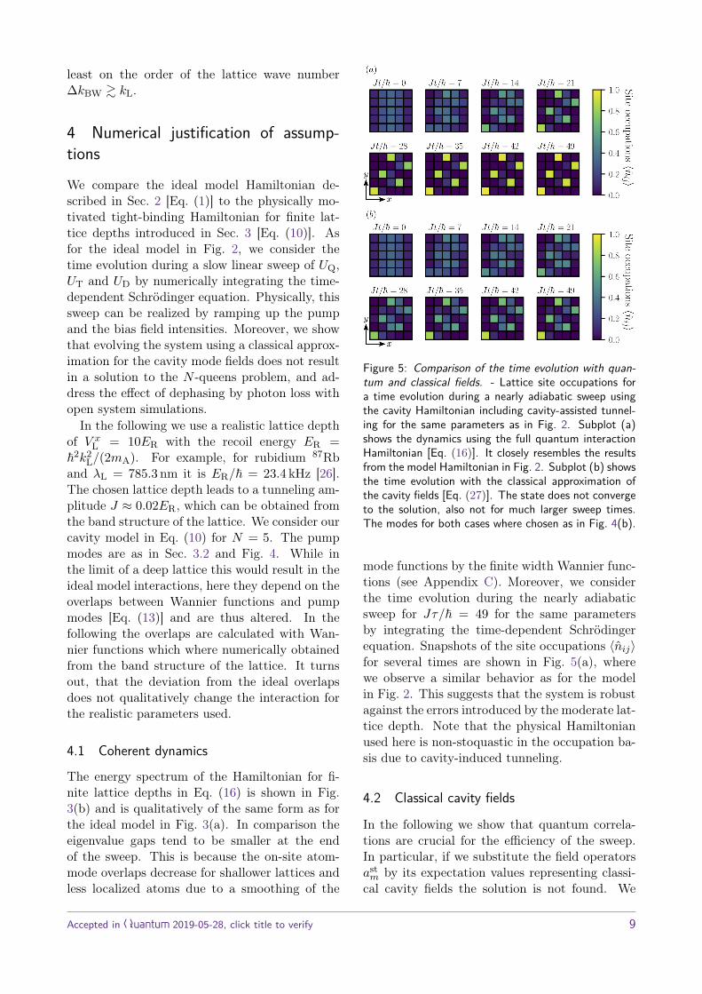
Figure 5: Comparison of the time evolution with quan-tum and classical fields. - Lattice site occupations fora time evolution during a nearly adiabatic sweep usingthe cavity Hamiltonian including cavity-assisted tunnel-ing for the same parameters as in Fig. 2. Subplot (a)shows the dynamics using the full quantum interactionHamiltonian [Eq. (16)]. It closely resembles the resultsfrom the model Hamiltonian in Fig. 2. Subplot (b) showsthe time evolution with the classical approximation ofthe cavity fields [Eq. (27)]. The state does not convergeto the solution, also not for much larger sweep times.The modes for both cases where chosen as in Fig. 4(b).

mode functions by the finite width Wannier func-tions (see Appendix C). Moreover, we considerthe time evolution during the nearly adiabaticsweep for Jτ/~ = 49 for the same parametersby integrating the time-dependent Schrödingerequation. Snapshots of the site occupations 〈nij〉for several times are shown in Fig. 5(a), wherewe observe a similar behavior as for the modelin Fig. 2. This suggests that the system is robustagainst the errors introduced by the moderate lat-tice depth. Note that the physical Hamiltonianused here is non-stoquastic in the occupation ba-sis due to cavity-induced tunneling.

4.2 Classical cavity fields

In the following we show that quantum correla-tions are crucial for the efficiency of the sweep.In particular, if we substitute the field operatorsastm by its expectation values representing classi-

cal cavity fields the solution is not found. We

Accepted in Quantum 2019-05-28, click title to verify 9

consider the semi-classical Hamiltonian

Hclasscav =~

∑m

N2∆c,mη2m

∆2c,m + κ2

m

×(Θ†m〈Θm〉+ 〈Θ†m〉Θm − |〈Θm〉|2

),

(27)where the expectation values have to be calcu-lated self-consistently with the current atom statevector. This substitution amounts to consideringonly first order fluctuations around the mean ofΘm in Eq. (16).

Consequently, the dynamics are described bya differential equation which is non-linear in thestate vector |ψ〉. We numerically solve this equa-tion by self-consistently updating the expectationvalue in each time step. It turns out that even forvery long sweep times, using classical fields doesnot lead to a solution of the queens problem. Thetime evolution for Jτ/~ = 49 is depicted in Fig.5(b). The discrepancy shows the necessity of en-tangled light-matter states in our procedure.

4.3 Dephasing due to cavity field loss

Finally, motivated by experimental considera-tions, we consider the open system including pho-ton decay through the cavity mirrors. This sys-tem can be described by a master equation forthe atoms [54]

ρ =− i

~[Hkin +Heff

cav, ρ]

+∑m

N2η2mκm

∆2c,m + κ2

m

(2ΘmρΘ†m − Θ†mΘm, ρ

),

(28)where curly brackets denote the anti-commutator(see Appendix B). The model is suitable for ana-lyzing the dephasing close to the coherent regimebefore any steady state is reached.

More insight can be gained by rewriting itin the basis of scattering eigenstates |ν〉 withΘm|ν〉 = θνm|ν〉, which scatter a field ανm =

Nηm∆c,m+iκm

θνm. These states converge to the occu-pation states in the deep lattice limit. The timeevolution for the matrix elements ρµν = 〈µ|ρ|ν〉reads

ρµν =(−Γµν − iΩµν)ρµν

− iJ~∑k

(〈µ|B|k〉ρkν − 〈k|B|ν〉ρµk

)(29)

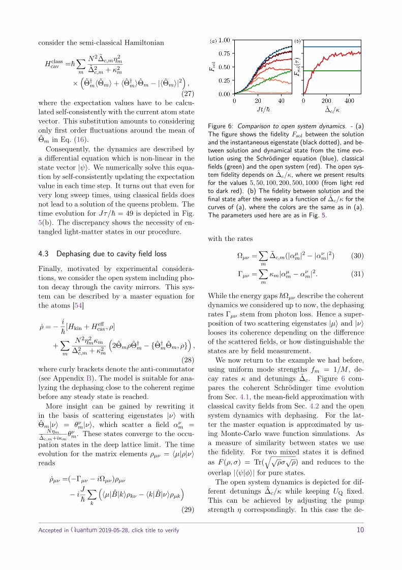
Figure 6: Comparison to open system dynamics. - (a)The figure shows the fidelity Fsol between the solutionand the instantaneous eigenstate (black dotted), and be-tween solution and dynamical state from the time evo-lution using the Schrödinger equation (blue), classicalfields (green) and the open system (red). The open sys-tem fidelity depends on ∆c/κ, where we present resultsfor the values 5, 50, 100, 200, 500, 1000 (from light redto dark red). (b) The fidelity between solution and thefinal state after the sweep as a function of ∆c/κ for thecurves of (a), where the colors are the same as in (a).The parameters used here are as in Fig. 5.

with the rates

Ωµν =∑m

∆c,m(|αµm|2 − |ανm|2) (30)

Γµν =∑m

κm|αµm − ανm|2. (31)

While the energy gaps ~Ωµν describe the coherentdynamics we considered up to now, the dephasingrates Γµν stem from photon loss. Hence a super-position of two scattering eigenstates |µ〉 and |ν〉looses its coherence depending on the differenceof the scattered fields, or how distinguishable thestates are by field measurement.

We now return to the example we had before,using uniform mode strengths fm = 1/M , de-cay rates κ and detunings ∆c. Figure 6 com-pares the coherent Schrödinger time evolutionfrom Sec. 4.1, the mean-field approximation withclassical cavity fields from Sec. 4.2 and the opensystem dynamics with dephasing. For the lat-ter the master equation is approximated by us-ing Monte-Carlo wave function simulations. Asa measure of similarity between states we usethe fidelity. For two mixed states it is definedas F (ρ, σ) = Tr(

√√ρσ√ρ) and reduces to the

overlap |〈ψ|φ〉| for pure states.The open system dynamics is depicted for dif-

ferent detunings ∆c/κ while keeping UQ fixed.This can be achieved by adjusting the pumpstrength η correspondingly. In this case the de-

Accepted in Quantum 2019-05-28, click title to verify 10

phasing rates

~ΓµνUQ

= κ

∆c

N2∑m

|θµm − θνm|2 (32)

go to zero for ∆c/κ 1. Thus, as ex-pected, the open system converges to the coher-ent Schrödinger dynamics in this limit (see Fig.6(b)).

Note that the coherence between states creat-ing similar fields is preserved much longer thanfor other states, which is expected to be impor-tant at the late stage of the sweep. For states withfixed similarity (e.g. one atom moved), |θµm−θνm|2is on the order of N−2, and thus the dephasingrates do not scale with N for such states.

5 Read-out

After the parameter sweep we need to determineif the obtained state is a solution or not. Thiscan in principle be done by reading out the fi-nal atomic state with single site resolution usinga quantum gas microscope [59, 60]. However, aswe consider an open system with the cavity out-put fields readily available, we will show that byproper measurements on the output light we candirectly answer this question without further ad-ditions. Note that after the sweep at the stageof the read-out, quantum coherences do not haveto be preserved since the solution is a classicalstate. This gives the freedom to increase the lat-tice depth to some high value in the deep latticeregime to suppress further tunneling, and to in-crease the pump power or decrease the detuningsin order to get a stronger signal at the detector.

5.1 Intensity measurement

For uniform cavity detunings, a state correspond-ing to the solution of the N -queens problem scat-ters less photons than all other states. Thus themeasurement of the total intensity in principleallows one to distinguish a solution from otherstates. To illustrate this we consider the totalrate of photons impinging on a detector scattered

by an atomic state |ψ〉

P (|ψ〉) =∑m

2κm〈(astm)†ast

m〉

=∑m

2κm∆c,m

∆c,mη2mN

2

∆2c,m + κ2

m

〈Θ†mΘm〉

≈UQζ

~∑ijkl

Aijkl〈nijnkl〉 = ζ

~〈Hdl

cav〉.

(33)In the last line we assumed that ζ = 2κm/∆c,m

does not depend on m and a deep lattice.Since P is proportional to the energy expec-

tation value, the ground state, i.e. the solutionof the queens problem, causes a minimal photonflux at the detector P0 = 3NUQζ. It stems fromthe on-site terms (i, j) = (k, l), where the fac-tor 3 comes from the three pump directions. Incontrast, each pair of queens violating the non-attacking condition in A leads to an increase ofthe photon flux by ∆P = 2UQζ. The two atomscreate an energy penalty for one another, explain-ing the factor 2. The relative difference of thephoton flux due to a state with L attacking pairsand a solution is given by

L∆PP0

= 2L3N . (34)

As this scales with 1/N it is difficult to distin-guish solutions from other states via measure-ment of the intensity for large N . Note thatfor non-uniform κm/∆c,m, photons from differentmodes have to be distinguished.

5.2 Field measurementMeasurement of the output field quadratures, forexample by homodyne detection, gives insightabout the absolute position of the atoms pro-jected onto the pump laser propagation direction.For the three directions used in our setup, thisyields the occupations of each column 〈Nx

i 〉 andeach diagonal 〈N+

i 〉 and 〈N−i 〉. Since a solution

of the queens problem has maximally one atomon each diagonal and exactly one atom on eachcolumn, it must fulfill

〈Nxi 〉 = 1 ∧ 〈N+

i 〉 ≤ 1 ∧ 〈N−i 〉 ≤ 1. (35)

The output field quadratures can thus be used todetermine if a classical final state is a solution ornot, which is the answer to the blocked diagonalsdecision problem we aim to solve. The signatures

Accepted in Quantum 2019-05-28, click title to verify 11

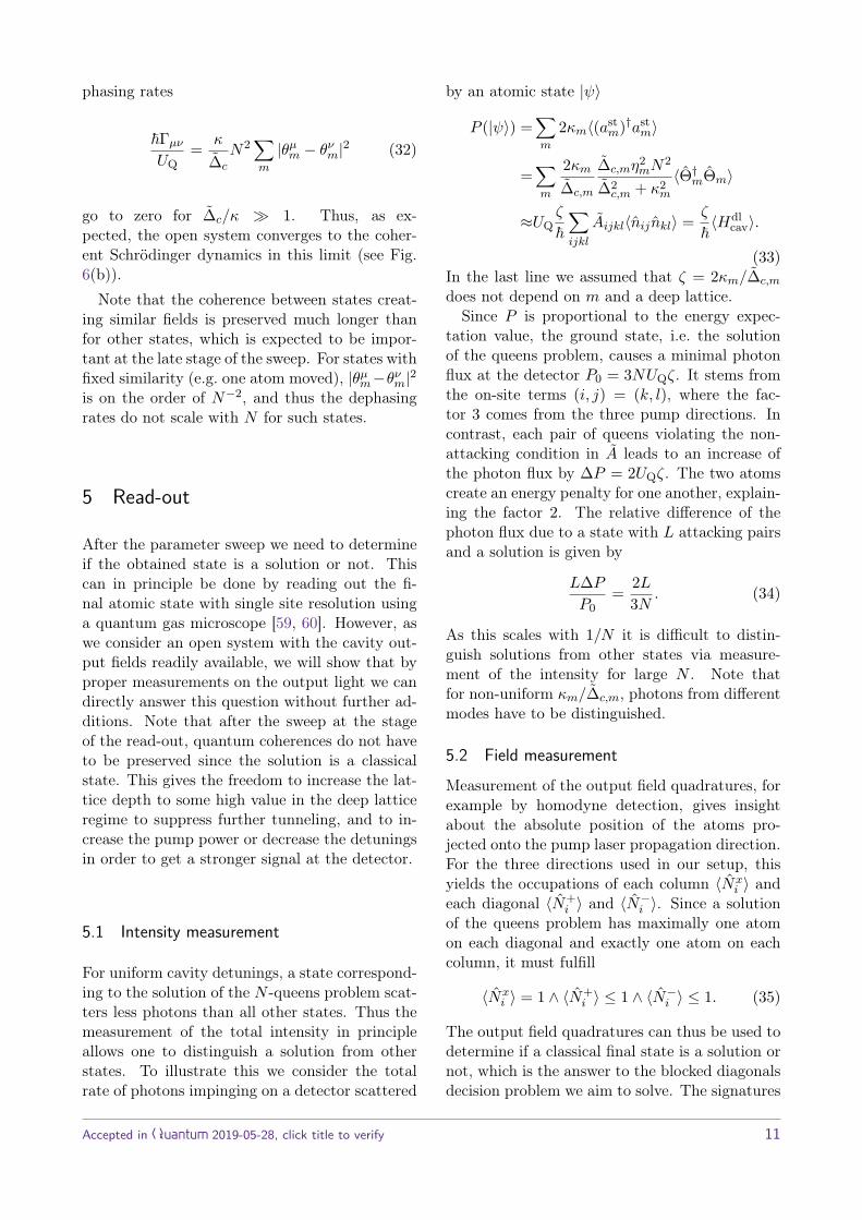
Figure 7: Signature of an atomic state in the cavity out-put. - In left and right column the signature of twodifferent atomic (pure) states are compared, whose oc-cupations are shown on the top (a). On the left there is asolution to the N -queens problem, while on the right oneatom was moved. (b) The polar plot shows the cavityfield expectation value 〈ast

m〉 in the complex plane. Mea-suring the fields by homodyne detection yields a certainquadrature of the field depending on the phase angleφ. An example is illustrated by the black line. (c) Themeasurable quadratures are shown for the example an-gle. The sequences can be Fourier transformed to obtainthe occupations of columns and of the diagonals. Theparameters used here are UQ = 5J and ∆c/κ = 10. Weused M = 2N − 1 = 9 modes per direction with wavenumbers as in Eq. (23). Different colors encode the dif-ferent directions of the pump modes: kx

m (blue), k+m

(green) and k−m (red). The lighter the color the larger

the wave number |kx,±m |.

of two example states in the cavity fields are de-picted in Fig. 7.

Let us illustrate the measurement by consid-ering only light scattered from the x-directionwith incident wave vectors kxm. Since these planewaves are constant in y-direction, the atom-fieldoverlaps do not depend on j. Neglecting cavity-induced tunneling, the field quadratures for aphase difference φ are

Re(〈astm〉e−iφ) =

∑i

Re(

ηme−iφ

∆c,m + iκmvi1m

)〈Nx

i 〉,

(36)revealing that cavity fields are determined by the

total occupations of the columns Nxi =

∑j nij .

For at least N modes (M ≥ N) this systemof equations can be inverted yielding the columnoccupations 〈Nx

i 〉. By measuring the cavity out-put field quadratures scattered from the diagonalpump light we obtain the occupations of each di-agonal 〈N+

i 〉 and 〈N−i 〉. Inverting the system of

equations for diagonals demands at least as manypump modes as diagonals, that is 2N − 1. Inver-sion can also be done efficiently and intuitivelyby using a discrete Fourier transform and its in-verse. To reveal the Fourier relation, one has toexpress the vijm’s in Eq. (36) within the harmonic(or in the deep lattice) approximation (see Ap-pendix C). The so obtained approximate inver-sion formula also works well for realistic latticedepths.

Strictly speaking the condition in Eq. (35) issufficient only for classical configurations, like oc-cupation number basis states |φν〉. Some super-positions |ψ〉 =

∑ν cν |φν〉 which are no solu-

tions might also fulfill the above criterion, be-cause summands in the field expectation val-ues 〈ast

m〉 =∑ν |cν |2〈φν |ast

m|φν〉 can cancel eachother. For instance, for UT = 0 the solutionfrom our example in Fig. 2 |ψsol〉 = |1, 4, 2, 5, 3〉scatters the same fields 〈ast

m〉 as the superpo-sition |ψnosol〉 = (|ψ1

nosol〉 + |ψ2nosol〉)/

√2 with

|ψ1nosol〉 = |1, 3, 2, 5, 4〉 and |ψ2

nosol〉 = |1, 4, 5, 2, 3〉,both of which are no solution. In this notationthe state |i1, i2, ..., iN 〉 has one atom on each site(ij , j). However, these macroscopic superposi-tions are highly unstable. Even theoretically themeasurement back-action [41, 61] projects super-positions of states scattering different fields (suchas |ψnosol〉) to one of its constituents. The inclu-sion of measurement back-action due to contin-uous measurement might thus lead to intriguingphenomena beyond those presented here and issubject to future work.

We emphasize again that the measurements de-scribed above answer the question if we found asolution or not, which is the answer to the com-binatorial decision problem. The exact configu-ration of the final state can be measured withsingle site resolution as demonstrated in severalexperiments [59, 60].

Accepted in Quantum 2019-05-28, click title to verify 12

6 ConclusionsWe present a special purpose quantum simulatorwith the aim to solve variations of the N -queensproblem based on atoms in a cavity. This com-binatorial problem may serve as a benchmark tostudy a possible quantum advantage in interme-diate size near term quantum experiments. Fromthe algorithmic point of view, the problem is in-teresting for quantum advantage as it is provenNP-hard and instances can be found that are notsolvable with current state-of-the-art algorithms.From the implementation point of view, the pro-posed quantum simulator implements the queensproblem without overhead and thus a few tensof atoms are sufficient to enter the classically in-tractable regime. The proposed setup of atoms ina cavity fits the queens problem naturally as therequired infinite range interactions arise there in-herently. We find that by treating the light fieldclassically the simulation does not find the solu-tions suggesting that quantum effects like atom-field entanglement cannot be neglected. More-over, we investigate the influence of photon losson the coherence time.

The queens problem is formulated as a decisionproblem, asking whether there is a valid config-uration of queens or not given the excluded di-agonals and fixed queens. Remarkably, to answerthe decision problem, a read-out of the atom posi-tions is not required as the necessary informationis encoded in the light that leaves the cavity. Todetermine the position of the queens requires sin-gle site resolved read-out, which is also availablein several current experimental setups [59].

In this work we concentrated on the coherentregime. The driven-dissipative nature of the sys-tem provides additional features which can be ex-ploited for obtaining the ground state. For cer-tain regimes, cavity cooling [24, 62] can help tofurther reduce sweep times and implement errorcorrection. Moreover, the back action of the fieldmeasurement onto the atomic state can be usedfor preparing states [41].

Note that an implementation of the N -queensproblem for a gate-based quantum computer wasproposed in Ref. [63] aiming to find a solutionof the unconstrained N -queens problem. Ourwork in contrast employs an adiabatic protocoland intends to answer the question if a solutionexists given constraints of blocked diagonals oralready placed queens, which was shown to be

NP-complete and numerically hard [30].Acknowledgments. We thank I. Gent, C. Jef-

ferson and P. Nightingale for fruitful discus-sions. Simulations were performed using the opensource QuantumOptics.jl framework in Julia [64]and we thank D. Plankensteiner for related dis-cussions. V. T. and H. R. are supported by Aus-trian Science Fund Project No. I1697-N27. W.L. acknowledges funding by the Austrian Sci-ence Fund (FWF) through a START grant underProject No. Y1067-N27 and the SFB BeyondCProject No. F7108-N38, the Hauser-Raspe foun-dation, and the European Union’s Horizon 2020research and innovation program under grantagreement No. 817482 PasQuanS.

Accepted in Quantum 2019-05-28, click title to verify 13

References[1] Aram W Harrow and Ashley Montanaro.

Quantum computational supremacy. Nature,549(7671):203–209, 2017. DOI: 10.1038/na-ture23458.

[2] J Ignacio Cirac and Peter Zoller. Goals andopportunities in quantum simulation. Nat.Phys., 8(4):264–266, apr 2012. ISSN 1745-2473. DOI: 10.1038/nphys2275.

[3] Rainer Blatt and Christian F Roos. Quan-tum simulations with trapped ions. Na-ture Physics, 8(4):277–284, 2012. DOI:10.1038/nphys2252.

[4] Immanuel Bloch, Jean Dalibard, and SylvainNascimbene. Quantum simulations with ul-tracold quantum gases. Nat. Phys., 8(4):267–276, apr 2012. ISSN 1745-2473. DOI:10.1038/nphys2259.

[5] Alán Aspuru-Guzik and Philip Walther.Photonic quantum simulators. Na-ture Physics, 8(4):285–291, 2012. DOI:10.1038/nphys2253.

[6] Sylvain De Léséleuc, Sebastian Weber, Vin-cent Lienhard, Daniel Barredo, Hans Pe-ter Büchler, Thierry Lahaye, and AntoineBrowaeys. Accurate mapping of multi-level rydberg atoms on interacting spin-1/2 particles for the quantum simulationof ising models. Physical review letters,120(11):113602, 2018. DOI: 10.1103/Phys-RevLett.120.113602.

[7] Andrew A Houck, Hakan E Türeci, and JensKoch. On-chip quantum simulation with su-perconducting circuits. Nature Physics, 8(4):292–299, 2012. DOI: 10.1038/nphys2251.

[8] I. M. Georgescu, S. Ashhab, and FrancoNori. Quantum simulation. Rev. Mod.Phys., 86:153–185, Mar 2014. DOI:10.1103/RevModPhys.86.153.

[9] Mark Saffman. Quantum computing withatomic qubits and rydberg interactions:progress and challenges. Journal of PhysicsB: Atomic, Molecular and Optical Physics,49(20):202001, 2016. DOI: 10.1088/0953-4075/49/20/202001.

[10] John Preskill. Quantum computing in thenisq era and beyond. Quantum, 2:79, 2018.DOI: 10.22331/q-2018-08-06-79.

[11] Sergio Boixo, Sergei V Isakov, Vadim NSmelyanskiy, Ryan Babbush, Nan Ding,Zhang Jiang, Michael J Bremner, John M

Martinis, and Hartmut Neven. Character-izing quantum supremacy in near-term de-vices. Nature Physics, 14(6):595, 2018. DOI:10.1038/s41567-018-0124-x.

[12] John Preskill. Quantum computing andthe entanglement frontier. arXiv:1203.5813[quant-ph], 2012.

[13] Hannes Bernien, Sylvain Schwartz, Alexan-der Keesling, Harry Levine, Ahmed Omran,Hannes Pichler, Soonwon Choi, Alexander SZibrov, Manuel Endres, Markus Greiner,et al. Probing many-body dynamics on a 51-atom quantum simulator. Nature, 551(7682):579, 2017. DOI: 10.1038/nature24622.

[14] Kihwan Kim, M-S Chang, Simcha Korenblit,Rajibul Islam, Emily E Edwards, James KFreericks, G-D Lin, L-M Duan, and Christo-pher Monroe. Quantum simulation of frus-trated ising spins with trapped ions. Nature,465(7298):590–593, 2010. DOI: 10.1038/na-ture09071.

[15] Peter Schauß, Marc Cheneau, Manuel En-dres, Takeshi Fukuhara, Sebastian Hild,Ahmed Omran, Thomas Pohl, ChristianGross, Stefan Kuhr, and Immanuel Bloch.Observation of spatially ordered structuresin a two-dimensional rydberg gas. Nature,491(7422):87–91, 2012. DOI: 10.1038/na-ture11596.

[16] Tadashi Kadowaki and Hidetoshi Nishimori.Quantum annealing in the transverse isingmodel. Phys. Rev. E, 58:5355–5363, Nov1998. DOI: 10.1103/PhysRevE.58.5355.

[17] Edward Farhi, Jeffrey Goldstone, Sam Gut-mann, and Michael Sipser. Quantum compu-tation by adiabatic evolution. arXiv:quant-ph/0001106, 2000.

[18] Tameem Albash and Daniel A Lidar. Adi-abatic quantum computation. Reviews ofModern Physics, 90(1):015002, 2018. DOI:10.1103/RevModPhys.90.015002.

[19] Andrew Lucas. Ising formulations of manynp problems. Frontiers in Physics, 2:5, 2014.DOI: 10.3389/fphy.2014.00005.

[20] Sergio Boixo, Troels F Rønnow, Sergei VIsakov, Zhihui Wang, David Wecker,Daniel A Lidar, John M Martinis, andMatthias Troyer. Evidence for quantumannealing with more than one hundredqubits. Nature Physics, 10(3):218, 2014.DOI: 10.1038/nphys2900.

Accepted in Quantum 2019-05-28, click title to verify 14

[21] Philipp Hauke, Helmut G Katzgraber, Wolf-gang Lechner, Hidetoshi Nishimori, andWilliam D Oliver. Perspectives of quantumannealing: Methods and implementations.arXiv:1903.06559 [quant-ph], 2019.

[22] Wolfgang Lechner, Philipp Hauke, and Pe-ter Zoller. A quantum annealing architecturewith all-to-all connectivity from local inter-actions. Science Advances, 1(9), 2015. DOI:10.1126/sciadv.1500838.

[23] Vicky Choi. Minor-embedding in adia-batic quantum computation: I. the param-eter setting problem. Quantum Informa-tion Processing, 7(5):193–209, 2008. DOI:10.1007/s11128-008-0082-9.

[24] Helmut Ritsch, Peter Domokos, FerdinandBrennecke, and Tilman Esslinger. Coldatoms in cavity-generated dynamical opti-cal potentials. Reviews of Modern Physics,85(2):553, 2013. DOI: 10.1103/RevMod-Phys.85.553.

[25] Christoph Maschler and Helmut Ritsch.Cold atom dynamics in a quantum opti-cal lattice potential. Physical review letters,95(26):260401, 2005. DOI: 10.1103/Phys-RevLett.95.260401.

[26] Renate Landig, Lorenz Hruby, Nishant Do-gra, Manuele Landini, Rafael Mottl, To-bias Donner, and Tilman Esslinger. Quan-tum phases from competing short-and long-range interactions in an optical lattice. Na-ture, 532(7600):476, 2016. DOI: 10.1038/na-ture17409.

[27] Igor B Mekhov and Helmut Ritsch. Quan-tum optics with ultracold quantum gases:towards the full quantum regime of thelight–matter interaction. Journal of PhysicsB: Atomic, Molecular and Optical Physics,45(10):102001, 2012. DOI: 10.1088/0953-4075/45/10/102001.

[28] Santiago F Caballero-Benitez, Gabriel Maz-zucchi, and Igor B Mekhov. Quantumsimulators based on the global collectivelight-matter interaction. Physical ReviewA, 93(6):063632, 2016. DOI: 10.1103/Phys-RevA.93.063632.

[29] Jordan Bell and Brett Stevens. A surveyof known results and research areas for n-queens. Discrete Mathematics, 309(1):1–31,2009. DOI: 10.1016/j.disc.2007.12.043.

[30] Ian P Gent, Christopher Jefferson, and Pe-

ter Nightingale. Complexity of n-queenscompletion. Journal of Artificial Intelli-gence Research, 59:815–848, 2017. DOI:10.1613/jair.5512.

[31] Itay Hen. Realizable quantum adia-batic search. EPL (Europhysics Letters),118(3):30003, 2017. DOI: 10.1209/0295-5075/118/30003.

[32] Itay Hen and Federico M Spedalieri. Quan-tum annealing for constrained optimization.Physical Review Applied, 5(3):034007, 2016.DOI: 10.1103/PhysRevApplied.5.034007.

[33] Peter Domokos and Helmut Ritsch. Collec-tive cooling and self-organization of atomsin a cavity. Physical review letters, 89(25):253003, 2002. DOI: 10.1103/Phys-RevLett.89.253003.

[34] Adam T Black, Hilton W Chan, and VladanVuletić. Observation of collective frictionforces due to spatial self-organization ofatoms: from rayleigh to bragg scattering.Physical review letters, 91(20):203001, 2003.DOI: 10.1103/PhysRevLett.91.203001.

[35] Varun D Vaidya, Yudan Guo, Ronen MKroeze, Kyle E Ballantine, Alicia J Kol-lár, Jonathan Keeling, and Benjamin L Lev.Tunable-range, photon-mediated atomic in-teractions in multimode cavity qed. Phys-ical Review X, 8(1):011002, 2018. DOI:10.1103/PhysRevX.8.011002.

[36] Subhadeep Gupta, Kevin L Moore, Kater WMurch, and Dan M Stamper-Kurn. Cav-ity nonlinear optics at low photon num-bers from collective atomic motion. Physi-cal review letters, 99(21):213601, 2007. DOI:10.1103/PhysRevLett.99.213601.

[37] Sarang Gopalakrishnan, Benjamin L Lev,and Paul M Goldbart. Frustration andglassiness in spin models with cavity-mediated interactions. Physical reviewletters, 107(27):277201, 2011. DOI:10.1103/PhysRevLett.107.277201.

[38] Sarang Gopalakrishnan, Benjamin L Lev,and Paul M Goldbart. Exploring mod-els of associative memory via cavityquantum electrodynamics. PhilosophicalMagazine, 92(1-3):353–361, 2012. DOI:10.1080/14786435.2011.637980.

[39] Sebastian Krämer and Helmut Ritsch. Self-ordering dynamics of ultracold atoms in mul-ticolored cavity fields. Physical Review A,

Accepted in Quantum 2019-05-28, click title to verify 15

90(3):033833, 2014. DOI: 10.1103/Phys-RevA.90.033833.

[40] Valentin Torggler, Sebastian Krämer, andHelmut Ritsch. Quantum annealing with ul-tracold atoms in a multimode optical res-onator. Physical Review A, 95(3):032310,2017. DOI: 10.1103/PhysRevA.95.032310.

[41] Igor B Mekhov and Helmut Ritsch. Quan-tum nondemolition measurements and statepreparation in quantum gases by lightdetection. Physical review letters, 102(2):020403, 2009. DOI: 10.1103/Phys-RevLett.102.020403.

[42] Vicky Choi. Minor-embedding in adia-batic quantum computation: Ii. minor-universal graph design. Quantum Informa-tion Processing, 10(3):343–353, 2011. DOI:10.1007/s11128-010-0200-3.

[43] Andrea Rocchetto, Simon C Benjamin, andYing Li. Stabilizers as a design tool fornew forms of the lechner-hauke-zoller an-nealer. Science advances, 2(10):e1601246,2016. DOI: 10.1126/sciadv.1601246.

[44] Alexander W Glaetzle, Rick MW van Bi-jnen, Peter Zoller, and Wolfgang Lechner.A coherent quantum annealer with rydbergatoms. Nature Communications, 8:15813,2017. DOI: 10.1038/ncomms15813.

[45] Walter Vinci and Daniel A Lidar. Scalableeffective-temperature reduction for quantumannealers via nested quantum annealing cor-rection. Physical Review A, 97(2):022308,2018. DOI: 10.1103/PhysRevA.97.022308.

[46] Layla Hormozi, Ethan W Brown, GiuseppeCarleo, and Matthias Troyer. Nonstoquas-tic hamiltonians and quantum annealing ofan ising spin glass. Physical Review B,95(18):184416, 2017. DOI: 10.1103/Phys-RevB.95.184416.

[47] Tameem Albash. Role of nonstoquastic cat-alysts in quantum adiabatic optimization.Physical Review A, 99(4):042334, 2019. DOI:10.1103/PhysRevA.99.042334.

[48] Sergei V Isakov, Guglielmo Mazzola,Vadim N Smelyanskiy, Zhang Jiang, SergioBoixo, Hartmut Neven, and MatthiasTroyer. Understanding quantum tun-neling through quantum monte carlosimulations. Physical review letters, 117(18):180402, 2016. DOI: 10.1103/Phys-RevLett.117.180402.

[49] Joel Klassen and Barbara M. Terhal. Two-local qubit Hamiltonians: when are theystoquastic? Quantum, 3:139, May 2019.ISSN 2521-327X. DOI: 10.22331/q-2019-05-06-139.

[50] Milad Marvian, Daniel A Lidar, and ItayHen. On the computational complexity ofcuring non-stoquastic hamiltonians. Naturecommunications, 10(1):1571, 2019. DOI:10.1038/s41467-019-09501-6.

[51] Immanuel Bloch. Ultracold quantum gasesin optical lattices. Nature Physics, 1(1):23–30, 2005. DOI: doi.org/10.1038/nphys138.

[52] Florian Meinert, Manfred J Mark, EmilKirilov, Katharina Lauber, Philipp Wein-mann, Michael Gröbner, Andrew J Daley,and Hanns-Christoph Nägerl. Observationof many-body dynamics in long-range tun-neling after a quantum quench. Science, 344(6189):1259–1262, 2014. DOI: 10.1126/sci-ence.1248402.

[53] Peter Domokos and Helmut Ritsch. Me-chanical effects of light in optical resonators.JOSA B, 20(5):1098–1130, 2003. DOI:10.1364/JOSAB.20.001098.

[54] Christoph Maschler, Igor B Mekhov, andHelmut Ritsch. Ultracold atoms in opticallattices generated by quantized light fields.The European Physical Journal D, 46(3):545–560, 2008. DOI: 10.1140/epjd/e2008-00016-4.

[55] Dieter Jaksch, Christoph Bruder, Juan Ig-nacio Cirac, Crispin W Gardiner, and PeterZoller. Cold bosonic atoms in optical lat-tices. Physical Review Letters, 81(15):3108,1998. DOI: 10.1103/PhysRevLett.81.3108.

[56] Walter Kohn. Analytic properties of blochwaves and wannier functions. Physical Re-view, 115(4):809, 1959. DOI: 10.1103/Phys-Rev.115.809.

[57] D Nagy, P Domokos, A Vukics, andH Ritsch. Nonlinear quantum dynamicsof two bec modes dispersively coupled byan optical cavity. The European Phys-ical Journal D, 55(3):659, 2009. DOI:10.1140/epjd/e2009-00265-7.

[58] Hessam Habibian, André Winter, SimonePaganelli, Heiko Rieger, and Giovanna Mo-rigi. Bose-glass phases of ultracold atomsdue to cavity backaction. Physical re-

Accepted in Quantum 2019-05-28, click title to verify 16

view letters, 110(7):075304, 2013. DOI:10.1103/PhysRevLett.110.075304.

[59] Waseem S Bakr, Jonathon I Gillen, AmyPeng, Simon Fölling, and Markus Greiner.A quantum gas microscope for detecting sin-gle atoms in a hubbard-regime optical lat-tice. Nature, 462(7269):74, 2009. DOI:10.1038/nature08482.

[60] Jacob F Sherson, Christof Weitenberg,Manuel Endres, Marc Cheneau, ImmanuelBloch, and Stefan Kuhr. Single-atom-resolved fluorescence imaging of an atomicmott insulator. Nature, 467(7311):68, 2010.DOI: 10.1038/nature09378.

[61] H. Carmichael. An Open Systems Approachto Quantum Optics: Lectures Presented atthe Université Libre de Bruxelles, October28 to November 4, 1991. Number Bd. 18in An Open Systems Approach to QuantumOptics: Lectures Presented at the UniversitéLibre de Bruxelles, October 28 to November

4, 1991. Springer Berlin Heidelberg, 1993.ISBN 9783540566342.

[62] Matthias Wolke, Julian Klinner, HansKeßler, and Andreas Hemmerich. Cavitycooling below the recoil limit. Science,337(6090):75–78, 2012. DOI: 10.1126/sci-ence.1219166.

[63] Rounak Jha, Debaiudh Das, Avinash Dash,Sandhya Jayaraman, Bikash K Behera, andPrasanta K Panigrahi. A novel quan-tum n-queens solver algorithm and its sim-ulation and application to satellite com-munication using ibm quantum experience.arXiv:1806.10221 [quant-ph], 2018.

[64] Sebastian Krämer, David Plankensteiner,Laurin Ostermann, and Helmut Ritsch.Quantumoptics.jl: A julia frameworkfor simulating open quantum systems.Computer Physics Communications,pages –, 2018. ISSN 0010-4655. DOI:10.1016/j.cpc.2018.02.004.

Accepted in Quantum 2019-05-28, click title to verify 17

Appendix

A Instance parameters

Table 1 provides an overview of the chosen parameters for the exemplary linear parameter sweep inthe main text (Figs. 2, 3 and 5).

Parameter Symbol ValueSystem size N 5

Final queens interaction energy UQ J

Final excluded diagonals penalty UD 5JFinal trapping energy UT 2J

Sweep time τ 49~/JExcluded sum-diagonals 2, 3, 6, 9

Excluded difference-diagonals 1, 2, 8, 9Trapping sites (3, 5)

Number of modes per direction M 5

Table 1: Parameters of the exemplary instance used in the figures in the main text.

We now describe how we choose the parameters used in our example. For this we calculate theminimal gap and the overlap with the final solution for several parameters to find a region with largeminimal gap and large overlap. Note that this is only done to find good parameters for our smallexample, where we already know the solution. For large systems such a calculation would beyondclassical numerical capabilities, which is why the problem poses a potential application for a quantumsimulator.

The minimal gap in the spectrum (e.g. the one shown in Fig. 3) depends on the final queens in-teraction energy UQ, the final trapping energy UT, the tunneling amplitude J and the final excludeddiagonals penalty UD. To find proper values for these parameters we determine the minimal gap in awide parameter range. In order to get the minimal gap, some of the Hamiltonian’s lowest eigenenergiesare calculated for discrete time steps during the sweep. Subsequently, the minimum of the differencebetween the groundstate and the first exited state at all time steps is taken to be the minimal gap. Thevalues of the minimal gap have to be scrutinized carefully since its accuracy depends on the resolutionof the discrete time steps. Therefore a more detailed analysis of the minimal gap might require a morecareful analysis, especially for high interaction strengths.

To analyze how well the quantum system reproduces the solution of the N -queens problem we studythe overlap

F = | 〈φ|ψ〉 | (37)

between the state |φ〉 that corresponds to the solution of the chosen instance of the queens problemintroduced in Fig. 1 and the state at the end of an adiabatic sweep |ψ〉 (i.e. the ground state of ourspectrum on the right side). This is necessary because we do not switch off the kinetic Hamiltonianin our example, and thus the "perfect" solution is only obtained in the limit of large energy penaltiesUQ, UD and UT.

Figure 8(a) suggests that in order to increase the minimal gap the ratio UQ/UD has to be chosen assmall as possible. We vary the ratio by fixing UD and varying UQ. Therewith, Fig. 8(a) indicates thatUQ should be as small as possible. However, as it can be seen in Fig. 8(b), a small UQ also decreasesthe overlap with the solution and the physical system does not resemble the desired solution of thequeens problem anymore. We therefore have to make a compromise between a reasonably large overlapand an optimized minimal gap.

Accepted in Quantum 2019-05-28, click title to verify 18

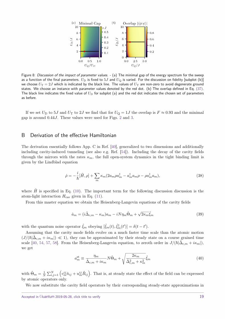
Figure 8: Discussion of the impact of parameter values. - (a) The minimal gap of the energy spectrum for the sweepas a function of the final parameters. UD is fixed to 5J and UQ is varied. For the discussion on fidelity [subplot (b)]we choose UT = 2J which is indicated by the black line. The values of UT are non-zero to avoid degenerate groundstates. We choose an instance with parameter values denoted by the red dot. (b) The overlap defined in Eq. (37).The black line indicates the fixed value of UD for subplot (a) and the red dot indicates the chosen set of parametersas before.

If we set UD to 5J and UT to 2J we find that for UQ = 1J the overlap is F ≈ 0.93 and the minimalgap is around 0.44J . These values were used for Figs. 2 and 3.

B Derivation of the effective Hamiltonian

The derivation essentially follows App. C in Ref. [40], generalized to two dimensions and additionallyincluding cavity-induced tunneling (see also e.g. Ref. [54]). Including the decay of the cavity fieldsthrough the mirrors with the rates κm, the full open-system dynamics in the tight binding limit isgiven by the Lindblad equation

ρ = − i~

[H, ρ] +∑m

κm(2amρa†m − a†mamρ− ρa†mam), (38)

where H is specified in Eq. (10). The important term for the following discussion discussion is theatom-light interaction Hcav given in Eq. (11).

From this master equation we obtain the Heisenberg-Langevin equations of the cavity fields

am = (i∆c,m − κm)am − iNηmΘm +√

2κmξm (39)

with the quantum noise operator ξm obeying [ξm(t), ξ†m(t′)] = δ(t− t′).Assuming that the cavity mode fields evolve on a much faster time scale than the atomic motion

(J/(~|∆c,m + iκm|) 1), they can be approximated by their steady state on a course grained timescale [40, 54, 57, 58]. From the Heisenberg-Langevin equation, to zeroth order in J/(~|∆c,m + iκm|),we get

astm ≡

ηm

∆c,m + iκmNΘm +

√2κm

∆2c,m + κ2

m

ξm (40)

with Θm = 1N

∑Ni,j=1

(vijmnij + uijmBij

). That is, at steady state the effect of the field can be expressed

by atomic operators only.We now substitute the cavity field operators by their corresponding steady-state approximations in

Accepted in Quantum 2019-05-28, click title to verify 19

the Heisenberg equation of the atomic annihilation operators

bij = 1i~

[bij , Hcav] + ... =− i∑m

(Nηm)2

∆2c,m + κ2

m

[∆c,m

([bij , Θ†m]Θm + Θ†m[bij , Θm]

)−iκm

([bij , Θ†m]Θm − Θ†m[bij , Θm]

)]− i

∑m

Nηm√

2κm√∆2c,m + κ2

m

([bij , Θ†m]ξm + ξ†m[bij , Θm]

) (41)

where we only report terms including the cavity. At this point, ordering of atomic and field operatorsbecomes important, since ast

m ∝ Θm as opposed to am does not necessarily commute with atomicoperators. Here we choose normal ordering, as already done in Eq. (11). The expression containscoherent terms proportional to ∆c,m and incoherent terms proportional to κm.

For |∆c,m| κm we can neglect the incoherent part and the Heisenberg equation can be obtainedfrom

bij = 1i~

[bij , Heffcav] + ... (42)

Thus the dynamics in the coherent regime is described by the effective Hamiltonian Heffcav given in Eq.

(16). Otherwise the Heisenberg equation is equivalent to the master equation (28).The results can also be obtained by naively substituting am with ast

m directly in the Hamiltonian Eq.(11) or the master equation (38) with the given ordering.

Note that the effective Hamiltonian can also be written in the form

Heffcav = ~

∑m

∆c,m(astm)†ast

m, (43)

which allows for a simple interpretation: For ∆c,m > 0 the lowest energy states tend to minimize theintensity of the cavity fields 〈(ast

m)†astm〉.

C Harmonic approximation of potential wellsIn this section we investigate the limit of a deep lattice in more detail. In Section 3.1 we presentedresults in the "infinitely" deep lattice limit, where the Wannier functions become delta functions. Togain more insight to deep but finite lattice depths, we use a harmonic approximation for the potentialwells. The ground state wave function is then an approximation to the lowest-band Wannier function

whar(x) = π−14a− 1

20 e

− x22a2

0 (44)

with the size a0 = (ER/VL)1/4/kL [55].With this the atom-mode overlap integrals [Eq. (13)] can be calculated analytically using running

wave mode functions [Eq. (18)]. For the on-site term we obtain

vijm = hm(xi, yj)e−(kxm2kL

)2√ERVL . (45)

It consists of the mode function at the lattice site and an exponential which reduces the overlap dueto Gaussian smoothing of the mode function. As intuitively expected, the smoothing has a strongereffect for large mode wave numbers kxm. For VL/ER 1, we obtain vi,jm = hm(xi, yj), as in the maintext.

For the off-site overlaps we obtain

uijm =hm((xi + xi+1)/2, yj)e−(kxm2kL

)2√ERVL e

−π24

√VLER .

(46)

Accepted in Quantum 2019-05-28, click title to verify 20

The overlap consists of three terms: First, it is the mode function evaluated in between the latticesites. Second, there is again the Gaussian smoothing term as for the on-site overlap. Lastly, there isan exponential independent of the modes, which comes from the overlap of the two Gaussians. It goesto zero for VL/ER 1, leading to uijm = 0.

The order operator is then

Θharm = 1

Ne−(kxm2kL

)2√ERVL

N∑i,j=1

hm(xi, yj)nij + hm((xi + xi+1)/2, yj)Bije−π

24

√VLER

(47)

leading to an interaction Hamiltonian [Eq. (16)] given by

Hharcav =UQ

∑m

fme−2(kxm2kL

)2√ERVL∑ijkl

h∗m(xi, yj)nij + h∗m((xi + xi+1)/2, yj)Bije−π

24

√VLER

×

hm(xk, yl)nkl + hm((xk + xk+1)/2, yl)Bkle−π

24

√VLER

,(48)

which in the "infinitely" deep lattice limit simplifies to Eq. (17). All cavity-induced tunneling termsare suppressed by the exponential and tend to be smaller than density-density terms. Also, since UQis maximally on the order of J (at the end of the sweep), cavity-induced tunneling terms are smallerthan Hkin. However, also the density-density terms can be small for example when hm(xi, yj) = 0,which is why we still include cavity-induced tunneling in the simulations.

In the main text we chose uniform fm = 1/M . To compensate for Gaussian smoothing one mightwant to include the exponential as correction

fm = fme2(kxm2kL

)2√ERVL , (49)

which leads to even better results (A is closer to A for finite lattice depths). Note that this correctiondoes only depend on VL and not on the problem size or number of modes in our implementation, sincethe range of kxm is fixed.

D Shape of the interactionHere we reformulate the interaction in the infinitely deep lattice limit from Eq. 22 with Fourier trans-forms by defining a real envelope function f(k) such that f(km) = fm. To get back the discrete wavenumbers, this function is sampled with a Dirac comb at the lines m∆k+ ks with m ∈ Z, where ks is aconstant shift and ∆k is the spacing between the pumped modes. In the main text we only considerthe case ks = 0 for simplicity. We define the Fourier transform as Ff(r) =

∫∞−∞ dkf(k)eikr/

√2π

and denote the convolution as (f ∗ g)(t) =∫∞−∞ f(τ)g(t− τ)dτ .

For simplicity, we take parallel wave vectors km. Along this direction r ‖ km we write

A(r) =∑m

fm cos(kmr) =∫ ∞−∞

dk f(k)∞∑

m=−∞δ(k −m∆k − ks) cos(kr)

= Re[√

2πFf(k)

∞∑m=−∞

δ(k −m∆k − ks)

(r)]

= Re

√2πFf(r) ∗∞∑

l=−∞δ

(r − l 2π

∆k

)eiksr

=

∞∑l=−∞

Re[√

2πFf(r − l 2π

∆k

)ei2πl

ks∆k

],

(50)where r = |r|. We used the convolution and shift theorem from Fourier analysis in the second to lastline and evaluated the convolution integrals by pulling out the sum in the last line.

Accepted in Quantum 2019-05-28, click title to verify 21

For symmetric envelopes centered around kc we can further simplify using the shift theorem

A(r) =∞∑

l=−∞

√2πFf

(r − l 2π

∆k

)cos

(kc

(r − l 2π

∆k

)+ 2πl ks∆k

), (51)

where f(k) = f(k+ kc) is the shifted envelope centered around k = 0, whose Fourier transform is real.Let us apply this to our example described in Section 3.2 and find out why the interaction has the

desired property given in equation Eq. (24). There we had uniform fm = 1/M and wave numbers

k0m = kL

(1 + 2m+ 1

2M

)(52)

with m = 0, ...,M−1. These have a mode spacing of ∆k = kL/M and are centered around kc = 3kL/2.One can see that only the odd modes of the cavity (wave numbers kn = n∆kFSR with n odd and freespectral range ∆kFSR) are used. Therefore, ∆k = 2∆kFSR and ks = ∆k/2, because the comb has tobe shifted to fit the odd modes. Due to the uniform fm the envelope is a rectangular function withwidth kL and height 1/M centered at kc

f(k) = rect((k − kc)/kL)/M =

1/M for k ∈ [kc − kL/2, kc + kL/2]0 otherwise.

(53)

The Fourier transform of a rectangular function centered around zero with unit width and heightis a sinc function sinc(x) = sin(x)/x. Using the addition theorem for the cosine and noting thatcos(πl) = (−1)l and sin(πl) = 0 we obtain an analytical expression for the interaction

A(r) =∞∑

l=−∞(−1)lsinc

(kL2

(r − l 2π

∆k

))cos

(kc

(r − l 2π

∆k

)). (54)

For l = 0 and at lattice site spacings rj = jπ/kL it takes the values

sinc(πj/2) cos(3πj/2) =

1 for j = 00 otherwise,

(55)

as desired. This comes from well known properties of sinc and cosine

sinc(πj/2) =

1 for j = 00 for j even(−1)

j−12 2

πj for j odd

cos(3πj/2) =

(−1)j2 for j even

0 for j odd.

The other summands have the same form, but are shifted by R = 2π/∆k = 2πM/kL = r2M (2Mlattice sites) and have alternating signs. Since R is an integer multiple of the lattice spacing this addsup to the desired interaction given in Eq. (24) in the main text.

Thus for rectangle envelopes the bandwidth ∆kBW determines the zeros of the interaction. Taking∆kBW = 2kL would lead to zeros at all lattice sites. For the smaller bandwidth ∆kBW = kL used here,only even sites become zero. This can be compensated by choosing a central wave number kc = nkL/2with n odd, which is responsible for the zeros at odd sites. The mode spacing ∆k determines the peakdistance. Finally, using odd cavity modes (specifying ks) leads to alternating peaks, which does nothave an effect in our implementation, since −2M < j < 2M .

Accepted in Quantum 2019-05-28, click title to verify 22