A quantitative theory of human color choices - Institute for

IMBS Technical Report # MBS 12-‐03

1

A quantitative theory of human color choices Natalia L. Komarova1,* and Kimberly A. Jameson2 1 Department of Mathematics, 2 Institute for Mathematical and Behavioral Sciences, University of California Irvine, Irvine CA 92697 * Corresponding author: [email protected], tel. 949-‐824-‐1268 Abstract. The system for colorimetry adopted by the Commission Internationale de l’Eclairage (CIE) in 1931, along with its subsequent improvements, represents a family of light mixture models that has served well for many decades for stimulus specification and reproduction when highly controlled color standards are important. Still, with regard to color appearance many perceptual and cognitive factors are known to contribute to color similarity, and, in general, to all cognitive judgments of color. Using experimentally obtained odd-‐one-‐out triad similarity judgments from 52 observers, we demonstrate that CIE-‐based models can explain a good portion (but not all) of the color similarity data. Color difference quantified by CIELAB ∆E explained behavior in three conditions tested at levels of 81% (across all colors), 79% (across red colors), and 66% (across blue colors). We show that the unexplained variation cannot be ascribed to inter-‐ or intra-‐individual variations among the observers, and points to the presence of additional factors shared by the majority of responders. Based on this we create a quantitative model of a lexicographic semiorder type, which shows how different perceptual and cognitive influences can trade-‐off when making color similarity judgments. We show that by incorporating additional influences related to categorical and lightness and saturation factors, the model explains more of the triad similarity behavior, namely, 91% (all colors), 90% (reds), and 87% (blues). We conclude that distance in a CIE model is but the first of several layers in a hierarchy of higher-‐order cognitive influences that shape color triad choices. We further discuss additional mitigating influences outside the scope of CIE modeling, which can be incorporated in this framework, including well-‐known influences from language, stimulus set effects, and color preference bias. We also discuss universal and cultural aspects of the model as well as non-‐uniformity of the color space with respect to different cultural biases. Introduction Humans constantly experience environmental color and interact with color appearance in everyday life. Because the perceptual processing of color arose as an adaptation through biological and cultural evolution, scientific analyses of human color processing must involve many factors, including physical properties of color stimuli, the processing of physical reflectance features by the human visual system, and higher-‐order cognitive processing of color in human visual cortex. On the other


2

hand, modern scientific study of human interactions with color stimuli grew largely out of early engineering and technological applications where color specification and reproduction in industry are of crucial importance. As a result, a key emphasis in the early days of developing photograph and display technology was to provide methods to precisely define color appearance, and to do so in ways that were adequate for reproducing color across different formats (for example, to make sure that the exact appearance of the yellow of Kodak film packaging is maintained in all its marketed forms). A consequence of this applied emphasis was the founding of the international authority on light, illumination and color, established in 1913, known as the Commission Internationale de l’Eclairage (or CIE) which led to a 1922 report on colorimetry by the Optical Society of America, and subsequently the formalization of the CIE 1931 XYZ color specification and the 1931 CIE 2-‐degree standard observer color space and human color matching functions, as well as a series of subsequent standard observer color space refinements [1,2]. Given its originally intended use, it is amazing that CIE systems have served so well as models of complex color appearance computations. Still, it is well-‐recognized that other perceptual and cognitive factors also contribute to color similarity, and, in general, to all cognitive judgments of color. We know, for example, that individual variation in visual processing features result in nonuniform color perception across observers [3,4] and that those CIE models most widely used in the color perception literature (i.e., CIELAB and CIELUV) are not entirely perceptually uniform and they do not take into consideration many factors contributing to individual differences in color perception [5,6]. Although perceptually uniform spacing has not been forthcoming, CIELAB distances are still used in empirical investigations to choose stimuli across color space that, for example, are quantified to appear equal in perceptual qualities based on the CIELAB ∆E distance metric. Moreover, cultural and linguistic biases can significantly alter color similarity judgments [7,8]. Thus, various cognitive factors must be involved in color similarity judgments, but aside from technical extensions of CIELAB (e.g., [9,10]) there is no clear principled approach for incorporating these factors into the existing modeling framework given by the CIE. The present paper attempts to address this challenge by incorporating cognitive modeling features to extend the potential of CIE systems as the basis for color similarity relations. In this paper we investigate whether CIE models are a good predictor of human choice behavior in color similarity judgments. We use results from a color triad task. Color triad tasks require observers to choose from three-‐color samples the singleton that does not form a natural grouping, or “belong with”, the other two of samples provided. Such tasks have been used with the aim of understanding biological, psychophysical and cognitive constraints that guide the human responders in their choices [11,12,13]. Color triad judgments provide an approach to bridge the gap between color specification models (i.e., tristimulus light mixture and color order systems) and the modeling of cognitive color relations. Using color similarity choice


3

data we discuss the appropriateness and utility of a CIE-‐based approach when other forms of cognitive influence are involved in color triad choice or other cognitive color judgment data. We analyze triad data from subjects who provided color similarity judgments both across color categories (i.e., reds, yellows, greens, etc.) referred to below as “global colors”, and within color categories (i.e., judged similarity among samples of red colors, or judged similarity among blue colors) referred to as “local red” and “local blue” color sets. Our findings support the use of some features of CIE models as a cognitive color appearance model when the model is extended to include additional color space features that figure into the cognitive color judgments. To illustrate, we increase the complexity of the model used to predict respondents’ triad choice data, for example by modeling influences of language-‐based categorical constraints expected to influence color judgments, and further analyze the fit to the triad choice behavior. Our results suggest that CIE distance is but the first layer in a hierarchy of influences that shape triad choices. Other mitigating influences come from language, stimulus set effects, and color preference bias. Results Let us represent each color triad as a triangle in a three-‐dimensional CIE space. The likelihood for a given stimulus in one such triad to be chosen as an odd-‐one-‐out is, in the simplest null-‐model, dictated by the geometry of the triangle [7,8]. The “null-‐model” assumes this probability to be proportional to the inverse of length of the opposing edge of the triangle (raised to a power, α ). For example, for a triangle of colors with vertices A, B, and C, the probabilities for colors A, B and C to be chosen are given by

ProbA =1

Σ || BC ||α, ProbB =

1Σ || AC ||α

, ProbC =1

Σ || AB ||α, (1)

where Σ =|| AB ||−α + || BC ||−α + || AC ||−α . Applied to experimental triad items, this model produces, for each color stimulus, its probability to be chosen, which can be compared to the empirically observed probabilities given by responders’ choices. There are different ways this comparison can be implemented. We can vary: (a) the method of distance measurement, using a ∆E color difference index based on CIELAB, CIE94, or CIEDE2000 [2]; (b) the way the “winning” stimulus is chosen from the multitude of responses, the majority or the consensus; (c) color similarity relations can be based on choice data from all participants, from participants grouped by their color vision profile, or on data from individual observers. We varied all these factors to obtain the most comprehensive picture of the validity of the model (see Text S1). A convenient measure of the CIE model’s performance is the number of mismatches that it produces compared to the experimental observations, that is, the number of triads where CIE distances predict a different odd-‐one-‐out stimulus compared to that chosen by experimental participants. For the CIELAB distance measure, the majority calculation of the winning response and the full set of participants, the number of mismatches is 13, 15, and 24 for the global,


4

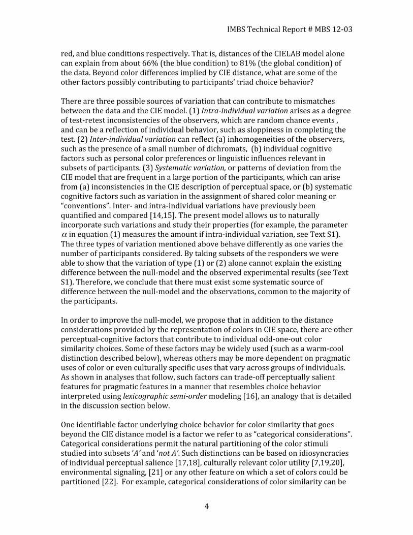
red, and blue conditions respectively. That is, distances of the CIELAB model alone can explain from about 66% (the blue condition) to 81% (the global condition) of the data. Beyond color differences implied by CIE distance, what are some of the other factors possibly contributing to participants’ triad choice behavior? There are three possible sources of variation that can contribute to mismatches between the data and the CIE model. (1) Intra-individual variation arises as a degree of test-‐retest inconsistencies of the observers, which are random chance events , and can be a reflection of individual behavior, such as sloppiness in completing the test. (2) Inter-individual variation can reflect (a) inhomogeneities of the observers, such as the presence of a small number of dichromats, (b) individual cognitive factors such as personal color preferences or linguistic influences relevant in subsets of participants. (3) Systematic variation, or patterns of deviation from the CIE model that are frequent in a large portion of the participants, which can arise from (a) inconsistencies in the CIE description of perceptual space, or (b) systematic cognitive factors such as variation in the assignment of shared color meaning or “conventions”. Inter-‐ and intra-‐individual variations have previously been quantified and compared [14,15]. The present model allows us to naturally incorporate such variations and study their properties (for example, the parameter α in equation (1) measures the amount if intra-‐individual variation, see Text S1). The three types of variation mentioned above behave differently as one varies the number of participants considered. By taking subsets of the responders we were able to show that the variation of type (1) or (2) alone cannot explain the existing difference between the null-‐model and the observed experimental results (see Text S1). Therefore, we conclude that there must exist some systematic source of difference between the null-‐model and the observations, common to the majority of the participants. In order to improve the null-‐model, we propose that in addition to the distance considerations provided by the representation of colors in CIE space, there are other perceptual-‐cognitive factors that contribute to individual odd-‐one-‐out color similarity choices. Some of these factors may be widely used (such as a warm-‐cool distinction described below), whereas others may be more dependent on pragmatic uses of color or even culturally specific uses that vary across groups of individuals. As shown in analyses that follow, such factors can trade-‐off perceptually salient features for pragmatic features in a manner that resembles choice behavior interpreted using lexicographic semi-order modeling [16], an analogy that is detailed in the discussion section below. One identifiable factor underlying choice behavior for color similarity that goes beyond the CIE distance model is a factor we refer to as “categorical considerations”. Categorical considerations permit the natural partitioning of the color stimuli studied into subsets ‘A’ and ‘not A’. Such distinctions can be based on idiosyncracies of individual perceptual salience [17,18], culturally relevant color utility [7,19,20], environmental signaling, [21] or any other feature on which a set of colors could be partitioned [22]. For example, categorical considerations of color similarity can be


5

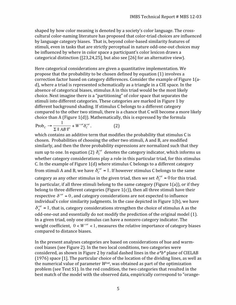
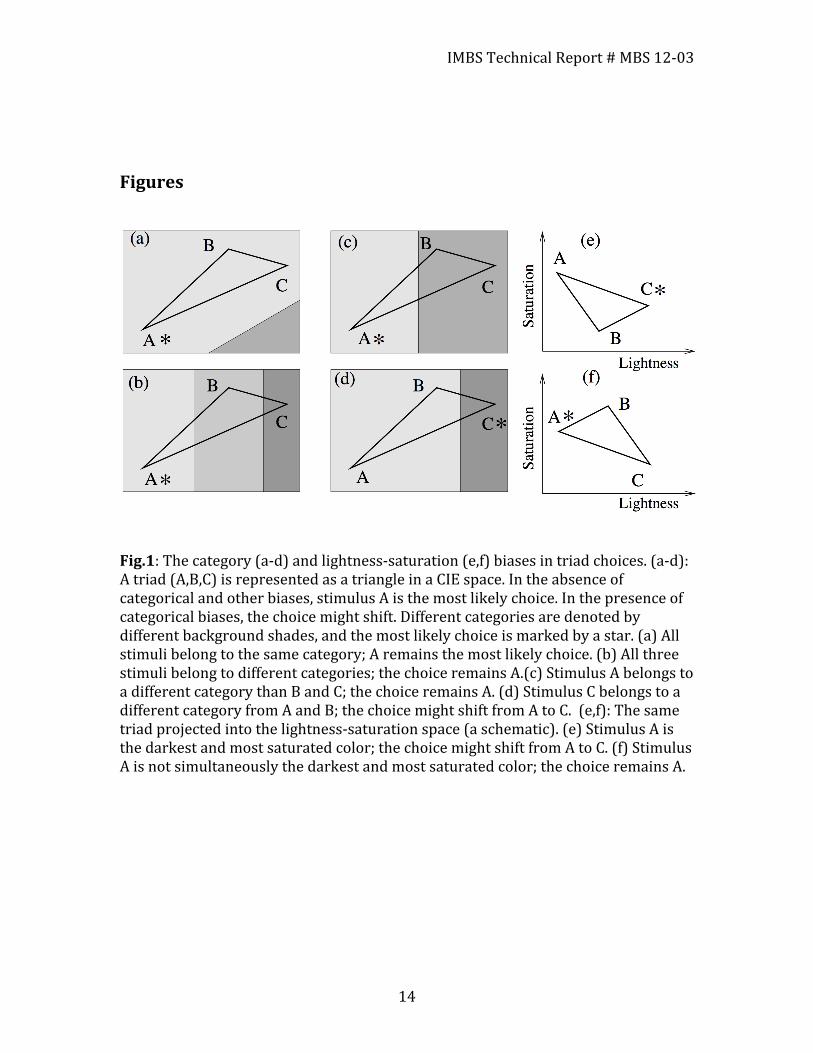
shaped by how color meaning is denoted by a society’s color language. The cross-‐cultural color-‐naming literature has proposed that color-‐triad choices are influenced by language category biases. That is, beyond color-‐based similarity features of stimuli, even in tasks that are strictly perceptual in nature odd-‐one-‐out choices may be influenced by where in color space a participant’s color lexicon draws a categorical distinction ([23,24,25], but also see [26] for an alternative view). Here categorical considerations are given a quantitative implementation. We propose that the probability to be chosen defined by equation (1) involves a correction factor based on category differences. Consider the example of Figure 1(a-‐d), where a triad is represented schematically as a triangle in a CIE space. In the absence of categorical biases, stimulus A in this triad would be the most likely choice. Next imagine there is a “partitioning” of color space that separates the stimuli into different categories. These categories are marked in Figure 1 by different background shading. If stimulus C belongs to a different category compared to the other two stimuli, there is a chance that C will become a more likely choice than A (Figure 1(d)). Mathematically, this is expressed by the formula

ProbC →1

Σ || AB ||α+W catδC

cat , (2)

which contains an additive term that modifies the probability that stimulus C is chosen. Probabilities of choosing the other two stimuli, A and B, are modified similarly, and then the three probability expressions are normalized such that they sum up to one. In equation (2) δC

cat denotes the category indicator, which informs us whether category considerations play a role in this particular triad, for this stimulus C. In the example of Figure 1(d) where stimulus C belongs to a different category from stimuli A and B, we have δC

cat = 1 . If however stimulus C belongs to the same category as any other stimulus in the given triad, then we set δC

cat = 0 for this triad. In particular, if all three stimuli belong to the same category (Figure 1(a)), or if they belong to three different categories (Figure 1(c)), then all three stimuli have their respective δ cat = 0 , and category considerations are not expected to influence individual’s color similarity judgments. In the case depicted in Figure 1(b), we have δAcat = 1 , that is, category considerations strengthen the choice of stimulus A as the

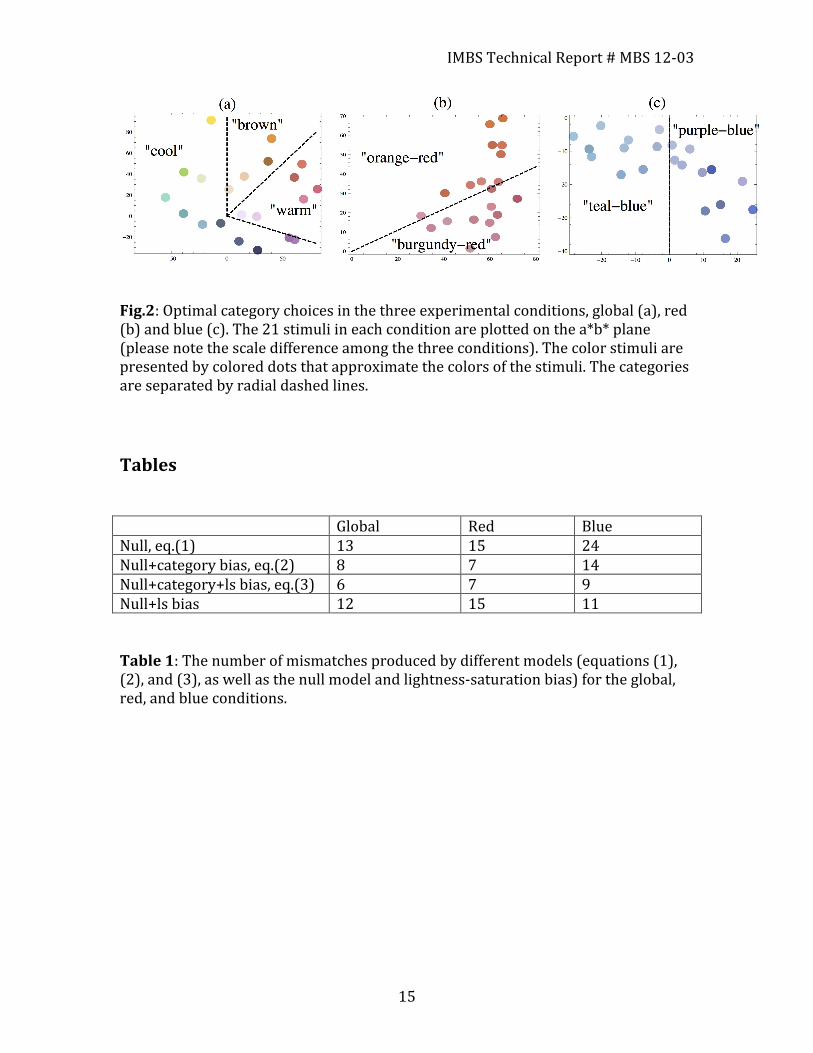
odd-‐one-‐out and essentially do not modify the prediction of the original model (1). In a given triad, only one stimulus can have a nonzero category indicator. The weight coefficient, , measures the relative importance of category biases compared to distance biases. In the present analyses categories are based on considerations of hue and warm-‐cool biases (see Figure 2). In the two local conditions, two categories were considered, as shown in Figure 2 by radial dashed lines in the a*b* plane of CIELAB (1976) space [1]. The particular choice of the location of the dividing lines, as well as the numerical value of parameter Wcat, was obtained as part of the optimization problem (see Text S1). In the red condition, the two categories that resulted in the best match of the model with the observed data, empirically correspond to “orange-‐

0 <W cat < 1


6

red” and “burgundy-‐red” biases. In the blue category, we have “teal-‐blue” and “purple-‐blue” biases. In the case of the global condition (Figure 2(a)) we find not two but three different categories termed as “warm”, “cool” and “brown”. As an aside, the emergence of a separate “brown” factor, or category, in these data is not surprising since browns differ from other colored light mixtures in that they exist as “relational colors” that are experienced in the context of a brighter surrounding field, and in CIELAB or CIELUV spaces correspond to “orange” color space coordinates [1], implying that “brown” light mixtures are absent from those models. Similarity judgments on “relational” colors like brown are possible in these data because surrounding contrast was supplied by the gray background used in our triad stimulus configuration [27]. When we apply this model to the data at hand, we observe that the category correction helps improve the performance of the model considerably, especially in the global and red conditions. The least number of mismatches that this model produces is 8, 7 and 14 for the global, red, and blue conditions respectively, see Table 1. We conclude that category constraints and distances are not the whole picture, which is especially apparent in the blue condition. Other factors must be at play. In order to find the source of the remaining variation, we explored the hypothesis that alternative dimensional differences can influence participants’ choices. We notice a common pattern in many of the mismatches in the blue condition: the CIE prediction of the odd-‐one-‐out stimulus corresponds to the color with the lowest lightness coordinate and the highest saturation coordinate compared to the other two stimuli in the triad, see Figure 1(b). We make a hypothesis that people prefer not to choose the darkest and the most saturated color as the odd-‐one-‐out. This leads to the following correction to model (2):

ProbA →1

Σ || BC ||α+W catδA

cat −W lsδAls , (3)

where the superscript “ls” refers to lightness-‐saturation bias, δAls is the lightness-‐saturation indicator, and 0 <W ls < 1 is the weight coefficient measuring the relative importance of the lightness-‐saturation bias (determined by a fitting procedure, see Text S1). As in equation (2), the other two probability values are modified similarly, and then normalized to make sure that they sum up to 1. In equation (3), the indicator δAls =1 only if stimulus A is the darkest and most saturated color of the three; it is zero otherwise, see Figure 1(e,f). In the Figure, we presented a possible projection of the triad ABC onto the lightness-‐saturation space. If, as in Figure 1(e), stimulus A happens to be the darkest and the most saturated color, then its lightness-‐saturated bias will be set to one, and it may lead to a different choice of the odd-‐one-‐out color. In other cases, such as the one illustrated in Figure 1(f), the lightness-‐saturation bias of stimulus A will be zero. We fitted the model in equation (3), and the best-‐fitting model reduces the number of mismatches to 6, 7 and 9 for the global, red and blue conditions respectively. Interestingly, in the global and red conditions, lightness-‐saturation bias does not make much of a difference. When


7

applied together with the category bias, or alone (see the last row of Table 1), it does not influence the number of mismatches significantly. In the blue condition however it plays an important role. When applied together with the category bias, it reduces the number of mismatches from 14 to 9, and when applied without the category bias, it reduces the number of mismatches from 24 to 11. To summarize, the most comprehensive model (3) can explain 91% of the data for the global, 90% for the red, and 87% for the blue condition. Discussion From the perspective of cognitive psychologists interested in understanding human color experience, the CIE models are perfect tools for empirical stimulus specification, but they are not ideal as models of the many ways humans experience and interact with color. Our results show that CIE color differences alone are insufficient to describe color similarity when strong sources of cognitive influence on color judgment are at play. This is because CIE formalizations were not designed to predict a variety of behavioral outcomes that arise from human color appearance processing. The formal geometric properties of CIE space do not very accurately predict human judgments of, for example, color similarity, color preference or color difference in complex scenes. The results presented here suggest that a family of models that use CIE distances in conjunction with other known perceptual and cognitive factors is a promising approach to using CIE formalisms as a basis for the quantitative modeling of cognitive color relations. The hierarchical nature of our model The present results confirm the suggestion (e.g., [10]) that the CIE formalization most frequently used to model observer’s judgments of color similarity and difference, is but one, albeit important, type of factor contributing to color choice behavior. To illustrate this we used features of color similarity (represented by distance in a “perceptually uniform” CIELAB model) as a predictor of choices in color triad tasks. We found that odd-‐one-‐out predictions based on CIELAB distances coincided with a good portion of the empirical data, and that above and beyond this other plausible factors, dimensions and attributes were found to contribute. When formally included in the model, these additional factors were found to substantially improve the predictions of the triad choice behavior. Our model can be considered a hierarchical model in the following sense. It includes the null model (the CIE distance model), which most of the time comprises the largest contribution to the choice probability. Other factors, although present, in the majority of cases do not have enough weight to modify the prediction given by the CIE distance model. In some cases, however, the CIE prediction is “weak”, which happens for example in the case when the triad is a nearly-‐equilateral triangle. In


8

this case, other linguistic or cognitive layers, such as category criteria or lightness-‐saturation baises, become the major basis for color similarity choices, and can determine the color choice behavior. These findings and this hierarchical modeling approach are related to lexicographic semi-order modeling of choice behavior [16]. In [16] Tversky states:

“… When faced with complex multidimensional alternatives … it is extremely difficult to utilize properly all the available information. Instead … people employ various approximation methods that enable them to process the relevant information in making a decision. The particular approximation scheme depends on the nature of the alternatives, as well as on the ways they are presented ... The lexicographic semiorder is one such approximation … ” ([16], p. 46).

Analogous to a lexicographic semi-‐order interpretation of these results, we found that people initially compare CIE distances as a first approximation to their triad choice decision. When the triple of distances among the three items compared were different enough, then people chose the most distant item of the triple as the odd-‐one-‐out. However, if the distance-‐based choice becomes ambiguous, then people could engage additional criteria in making a choice. This is in the same spirit as the model of interpoint-‐distance color category formation described previously [28,29]. Modeling color similarity judgments as a series of successive approximations that contribute to choice outcomes is, we believe, (i) a new and highly plausible approach to modeling the perceptual-‐cognitive-‐pragmatic aspects of stimuli that naturally play a role in color similarity judgments, and (ii) is an appropriate and useful extension of the formalisms presented by lexicographic semiorder modeling. CIE as a basis for our modeling approach It should be noted that in this paper we emphasize a modeling approach that is based on the most widely used index of color difference: CIELAB ∆E. We examined alternative models based on other more recently introduced CIE color difference equations (CIE94 and CIEDE2000, see Text S1) but these alternatives either were not too different from that found with CIELAB ∆E, or they did not produce much improvement (or decline) beyond that shown with CIELAB (resembling trends seen when color difference equations are compared in applications across a range of datasets). One way to improve the hierarchical cognitive modeling approach introduced here may be to build on one of the more complex parametric models of color appearance (i.e., CIECAM97, CIECAM02, CIECAM02-‐UCS) that have been developed by CIE scientists in the last decade. Although these more recent color appearance models (CAMs) strive to advance color difference estimation beyond CIELAB-‐based formulas, they remain under active development and are not considered final


9

models, as they continue to evolve, and continue as topics of ongoing testing, debate, and discussion [30]. Finally, the CAMs are dramatically more complex computationally, to the point of bordering on being impractical for some applications. This is likely the reason they have not been embraced widely as tools in the empirical research literatures that study behaviors linked to cognitive and perceptual color relations. These two reasons underlie our choice to emphasize and build on the accepted, widely used, color difference index CIELAB ∆E. However, once CAM development is finalized and vetted by CIE experts, a potentially useful pursuit might be to generalize our hierarchical approach by using a CAM as the starting point for computing distances – this is entirely compatible with the aims of the present paper, but is necessarily a task for future modeling research. The color space is non-uniform with respect to category and lightness-saturation biases Our analyses show that different warm-‐cool category and lightness-‐saturation emphases are found across global, red and blue triad choices (Table 1). What is the reason for this difference? One possibility is that such constructs may not be uniformly appropriate, or equally relevant, across the entire color space. For example, for some regions of color space, a categorical distinction of warm-‐cool may be a useful or meaningful distinction to make (e.g., [31,32]), and in other regions of the space, or for other subsets of stimuli, it may be less useful. Variation in the appropriateness of a given categorical distinction across color space can be linked to a range of factors outside the domain of the standard observer model that are likely to contribute to similarity judgments of color. Because such factors can be cognitive, cultural, linguistic, and so on, they are almost certainly beyond the scope of CIE modeling alone, and therefore not easily addressed even by further extending the latest, most advanced forms of CIE models. Our suggested analogy to lexicographic semiorder modeling within a hierarchy involving CIE modeling builds on CIE advances and allows many more factors to be accounted for and addressed. Note that categorical considerations modeled here could originate from any number of sources. They could arise from normal biological bases [32] or less common biologically-‐based deficiencies (e.g., color vision dichromacy); from culturally specific factors [19,20]; from putative environmental or ecological salience [33,34]; from social color utility (e.g., highly valued purple ink used to dye royal cloth in ancient societies) ([35], chapter 62); or from language-‐based marked/unmarked color relations [36]. In such cases categorical considerations need not be applied uniformly across the entire color space, and may only apply in subregions of color space. The only feature required of the categorical consideration as formalized here is that it provide a connected set ‘A’/‘not A’ partition in the color space on which color similarity judgments can be evaluated.


10

If limited appropriateness of categorical considerations across color space is possible, then it is not surprising that the present data shows warm-‐cool category considerations improve the fit to the data for global and red conditions, while they explain less of the data for the case of the blue condition. Similarly, the criteria of lightness and saturation seem to play a role in triad choice data for the blue condition but not for the red condition or the global condition. Such patterns are plausible because stimulus sets for the three conditions were not sampled to be subjectively equal on all possible dimensions. Thus, cognitive and perceptual salience may be differently represented by samples comprising the three stimulus sets (and it is clear that the global stimulus set already dramatically differs in the hue dimension compared to the red or blue stimulus sets). Universal and cultural components of the model One advantage of CIE modeling that keeps formalizations tractable is that a standard observer approach to color modeling is used. This standard observer simplification does, however, limit the potential to address systematic variation in observer groups that can be linked to, for example, shared knowledge about color, which uniquely contributes to color similarity relations in observers with specific linguistic or cultural affiliations. In these cases where culturally-‐relevant information is known, it would be beneficial to include such information as a factor relevant in color similarity judgments. Extending the modeling capabilities of the CIE in this way is one aim of the present hierarchical modeling approach. This article considers data only from native-‐language speakers of English. But it is certainly true that category influences on color triad choices will differ for non-‐English speakers. For example, one would expect variation in lightness-‐saturation influences on color triad choices across ethnolinguistic groups [37]. Thus, what we consider universal in this framework are the identifiable perceptual and cognitively salient features of chosen triad stimuli (i.e., distance in a color space captured by the null-‐model), and what is cultural are the alternative approximations that additionally contribute to triad choices (i.e., pragmatic, environmental, individual and other culturally dependent factors captured by the additional layers in our model). The universal-cultural contrast differs here from that typically seen in the literature – that is, although the two forms of influence arise from very different sources, they nevertheless can both contribute to odd-‐one-‐out color similarity judgments. Examples of how category influences can differ across language groups is readily available. Russian has two distinct linguistic categories (or two “basic color terms”) for colors that English denotes under the lexical category “blue” [7,8]. Similarly, Hungarian has two basic terms for “red” colors (piros and vörös) [38] and Hungarian speakers use category glosses for “light” and “dark” (világos and sötét, respectively) to modify basic color terms much more frequently than that seen in native English color naming. This suggests that there are differences of lightness dimension


11

salience between native-‐language Hungarian and English color naming [39]. Almost the opposite scenario is found in native-‐language Vietnamese speakers where one category term (i.e., xanh) is used for denoting all “greens” and “blues” and the linguistic differentiation of green appearances from blue appearances is only achieved by modifying terms that specify which xanh appearance is “green” (or xanh lá cây or “xanh like the leaves”) and which xanh is “blue” (or xanh nước biển or “xanh like the ocean”) [13]. Thus, linguistic and cultural factors could set which criteria are most attended to in color similarity judgments compared across cultures. Indeed, many forms of linguistic markedness could influence which criteria color similarity is based on, and these would be expected to vary across ethno-‐linguistic groups and might even arise due to subgroups within a linguistic culture, such as color experts (e.g., professional artists and designers) compared to individuals in the same ethno-‐linguistic culture with little color expertise. Materials and methods Data from 52 native English speakers (32 female and 20 male) are analyzed (see Text S1 for details). Participants were randomly presented series of triad trials comprised of three precisely rendered color stimuli. In a given triad trial participants must identify which of the three items presented is most different from the remaining two. Color appearance triads were judged separately for three color sets representing global, local red, and local blue color conditions. Each condition included 21 stimuli for a total of 70 triad judgments per condition. All experimental methods, procedures and stimuli were reported previously [11]. All further details are provided in Text S1.

Acknowledgement: Partial support was provided by National Science Foundation (NSF) grant NSF 07724228 from the Methodology, Measurement, and Statistics (MMS) Program of the Division of Social and Economic Sciences (SES).

References 1. Wysecki G, Stiles WS (1982) Color Science: Concepts and Methods, Quantitative

Data and Formulae. New York: Wiley. 2. Fairchild MD (2005) Color Appearance Models. Chichester, UK: Wiley-‐IS&T. 3. Helm CE, Tucker LR (1962) Individual differences in the structure of color-‐

perception. Am J Psychol 75: 437-‐444.


12

4. Webster MA, Miyahara E, Malkoc G, Raker VE (2000) Variations in normal color vision. II. Unique hues. J Opt Soc Am A Opt Image Sci Vis 17: 1545-‐1555.

5. Webster MA, MacLeod DI (1988) Factors underlying individual differences in the color matches of normal observers. J Opt Soc Am A 5: 1722-‐1735.

6. Díaz JA, Chiron A, Viénot F (1989) Tracing a Metameric Match to Individual Variations of Color Vision. Color Research & Application 23: 379-‐389.

7. Paramei GV (2005) Singing the Russian blues: an argument for culturally basic color terms. Cross-‐Cultural Research 39: 10-‐38.

8. Paramei GV (2007) Russian ‘blues’: Controversies of basicness. In: MacLaury RE, Paramei GV, Dedrick D, editors. Anthropology of Color: Interdisciplinary Multilevel Modeling. Amsterdam/Philadelphia: John Benjamins.

9. Fairchild MD, Berns RS (1993) Image color-‐appearance specification through extension of CIELAB. Color Research & Application 18: 178-‐190.

10. Zhang X, Silverstein DA, Farrell JE, Wandell BA. Color image quality metric S-‐CIELAB and its application on halftone texture visibility; 1997. pp. 44-‐48.

11. Sayim B, Jameson KA, Alvarado N, Szeszel MK (1988) Semantic and perceptual representations of color: Evidence of a shared color-‐naming function. Journal of Cognition and Culture 5: 427-‐486.

12. Paramei GV, Bimler DL, Cavonius CR (1998) Effect of luminance on color perception of protanopes. Vision Res 38: 3397-‐3401.

13. Jameson KA, Alvarado N (2003) Differences in color naming and color salience in Vietnamese and English. Color Research and Application 28: 113-‐138.

14. Bimler D, Kirkland J, Pichler S (2004) Escher in color space: Individual-‐differences multidimensional scaling of color dissimilarities collected with a gestalt formation task. Behavior Research Methods Instruments & Computers 36: 69-‐76.

15. Moore CC, Romney AK, Hsia TI (2000) Shared cognitive representations of perceptual and semantic structures of basic colors in Chinese and English. Proceedings of the National Academy of Sciences of the United States of America 97: 5007-‐5010.

16. Tversky A (1969) Intransitivity of Preferences. Psychological Review 76: 31-‐&. 17. Jameson KA, Komarova NL (2009) Evolutionary models of color categorization. I.

Population categorization systems based on normal and dichromat observers. J Opt Soc Am A Opt Image Sci Vis 26: 1414-‐1423.

18. Jameson KA, Komarova NL (2009) Evolutionary models of color categorization. II. Realistic observer models and population heterogeneity. J Opt Soc Am A Opt Image Sci Vis 26: 1424-‐1436.

19. Davidoff J, Davies I, Roberson D (1999) Colour categories in a stone-‐age tribe. Nature 398: 203-‐204.

20. Roberson D, Davies I, Davidoff J (2000) Color categories are not universal: Replications and new evidence from a stone-‐age culture. Journal of Experimental Psychology-‐General 129: 369-‐398.

21. Komarova NL, Jameson KA (2008) Population heterogeneity and color stimulus heterogeneity in agent-‐based color categorization. J Theor Biol 253: 680-‐700.


13

22. Baronchelli A, Gong T, Puglisi A, Loreto V (2010) Modeling the emergence of universality in color naming patterns. Proc Natl Acad Sci U S A 107: 2403-‐2407.

23. Goldstone R (1994) Influences of categorization on perceptual discrimination. Journal of Experimental Psychology-‐General 123: 178-‐200.

24. Gilbert AL, Regier T, Kay P, Ivry RB (2006) Whorf hypothesis is supported in the right visual field but not the left. Proceedings of the National Academy of Sciences of the United States of America 103: 489-‐494.

25. Regier T, Kay P, Cook RS (2005) Focal colors are universal after all. Proceedings of the National Academy of Sciences of the United States of America 102: 8386-‐8391.

26. Brown AM, Lindsey DT, Guckes KM (2011) Color names, color categories, and color-‐cued visual search: Sometimes, color perception is not categorical. Journal of Vision 11.

27. Bartleson CJ (1976) Brown. Color Research and Application 1: 181-‐191. 28. Jameson KA, D’Andrade RG (1997) It’s not really Red, Green, Yellow, Blue: An

Inquiry into Cognitive Color Space. In: Hardin CL, Maffi L, editors. Color Categories in Thought and Language. UK: Cambridge University Press. pp. 295-‐318.

29. Jameson KA (2005) Culture and Cognition: What is Universal about the Representation of Color Experience? . The Journal of Cognition & Culture 5: 293-‐347.

30. Fernandez-‐Maloigne C, editor (2013) Advanced Color Image Processing and Analysis: Springer.

31. Lindsey DT, Brown AM (2006) Universality of color names. Proc Natl Acad Sci U S A 103: 16608-‐16613.

32. Xiao Y, Kavanau C, Bertin L, Kaplan E (2011) The biological basis of a universal constraint on color naming: cone contrasts and the two-‐way categorization of colors. PLoS One 6: e24994.

33. Changizi MA, Zhang Q, Shimojo S (2006) Bare skin, blood and the evolution of primate colour vision. Biol Lett 2: 217-‐221.

34. Osorio D, Vorobyev M (1996) Colour vision as an adaptation to frugivory in primates. Proceedings of the Royal Society of London Series B-‐Biological Sciences 263: 593-‐599.

35. Bostock J, Riley HT (1855) The Natural History of Pliny, The Elder. London: Taylor and Francis.

36. Battistella E (1996) The Logic of Markedness. New York: Oxford University Press.

37. MacLaury RE, Hewes GW, Kinnear PR, Deregowski J, Merrifield WR, et al. (1992) From Brightness to Hue: An Explanatory Model of Color-‐Category Evolution. Current Anthropology 33: 137-‐186.

38. Berlin B, Kay P (1969) Basic Color Terms: Their Universality and Evolution Berkeley: University of California Press.

39. Barratt LB, Kontra M (1996) Matching Hungarian and English color terms. International Journal of Lexicography 9: 102-‐117.


14

Figures

Fig.1: The category (a-‐d) and lightness-‐saturation (e,f) biases in triad choices. (a-‐d): A triad (A,B,C) is represented as a triangle in a CIE space. In the absence of categorical and other biases, stimulus A is the most likely choice. In the presence of categorical biases, the choice might shift. Different categories are denoted by different background shades, and the most likely choice is marked by a star. (a) All stimuli belong to the same category; A remains the most likely choice. (b) All three stimuli belong to different categories; the choice remains A.(c) Stimulus A belongs to a different category than B and C; the choice remains A. (d) Stimulus C belongs to a different category from A and B; the choice might shift from A to C. (e,f): The same triad projected into the lightness-‐saturation space (a schematic). (e) Stimulus A is the darkest and most saturated color; the choice might shift from A to C. (f) Stimulus A is not simultaneously the darkest and most saturated color; the choice remains A.


15

Fig.2: Optimal category choices in the three experimental conditions, global (a), red (b) and blue (c). The 21 stimuli in each condition are plotted on the a*b* plane (please note the scale difference among the three conditions). The color stimuli are presented by colored dots that approximate the colors of the stimuli. The categories are separated by radial dashed lines. Tables Global Red Blue Null, eq.(1) 13 15 24 Null+category bias, eq.(2) 8 7 14 Null+category+ls bias, eq.(3) 6 7 9 Null+ls bias 12 15 11 Table 1: The number of mismatches produced by different models (equations (1), (2), and (3), as well as the null model and lightness-‐saturation bias) for the global, red, and blue conditions.

Text S1

Quantitative theory of human color choices

N.L. Komarova and K.A. Jameson

1 Experimental methods

1.1 Participants

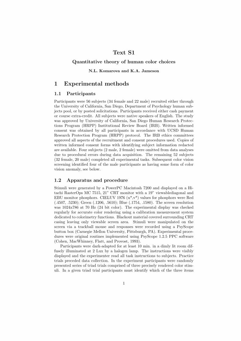
Participants were 56 subjects (34 female and 22 male) recruited either throughthe University of California, San Diego, Department of Psychology human sub-jects pool, or by posted solicitations. Participants received either cash paymentor course extra-credit. All subjects were native speakers of English. The studywas approved by University of California, San Diego Human Research Protec-tions Program (HRPP) Institutional Review Board (IRB). Written informedconsent was obtained by all participants in accordance with UCSD HumanResearch Protection Program (HRPP) protocol. The IRB ethics committeesapproved all aspects of the recruitment and consent procedures used. Copies ofwritten informed consent forms with identifying subject information redactedare available. Four subjects (2 male, 2 female) were omitted from data analysesdue to procedural errors during data acquisition. The remaining 52 subjects(32 female, 20 male) completed all experimental tasks. Subsequent color visionscreening identified four of the male participants as having some form of colorvision anomaly, see below.

1.2 Apparatus and procedure

Stimuli were generated by a PowerPC Macintosh 7200 and displayed on a Hi-tachi RasterOps MC 7515, 21” CRT monitor with a 19” viewablediagonal andEBU monitor phosphors. CIELUV 1976 (u*,v*) values for phosphors were Red(.4507, .5230); Green (.1206, .5610); Blue (.1754, .1580). The screen resolutionwas 1024x786 at 70 Hz (24 bit color). The experimental display was checkedregularly for accurate color rendering using a calibration measurement systemdedicated to colorimetry functions. Blackout material covered surrounding CRTcasing leaving only viewable screen area. Stimuli were manipulated on thescreen via a trackball mouse and responses were recorded using a PsyScopebutton box (Carnegie Mellon University, Pittsburgh, PA). Experimental proce-dures were original routines implemented using PsyScope 1.2.5 PPC software(Cohen, MacWhinney, Flatt, and Provost, 1993).

Participants were dark-adapted for at least 10 min. in a dimly lit room dif-fusely illuminated at 2 Lux by a halogen lamp. The instructions were visiblydisplayed and the experimenter read all task instructions to subjects. Practicetrials preceded data collection. In the experiment participants were randomlypresented series of triad trials comprised of three precisely rendered color stim-uli. In a given triad trial participants must identify which of the three items

1

presented is most different from the remaining two. Color appearance triadswere judged separately for the three conditions tested (i.e., global, local red andlocal blue). Each condition included 21 stimuli in a Balanced Incomplete Block

Design (BIBD, lambda = 1) for a total of 70 triad judgments per condition.A Balanced Incomplete Block Design (BIBD or BIB) is an established way

of reliably assessing a subset all possible triples among a number of items [20].BIBDs have been used extensively in the study of semantics in anthropology,clinical psychology and psychophysics as a technique for deriving informationabout structural relations among many items [4]. Such designs are importanttools in investigations of cognition, and can be traced back to mathematicalpsychologist C. H. Coombs [5]. Triad BIB designs are proven as alternativesto presenting participants a full complement of triads. Here a full complementof triadic comparisons for N = 21 items for a single conditions would be 1330triads (given by N(N − 1)(N − 2)/6, where each pair is presented with everyother item in the stimulus set). Requiring 1330 judgments for each of the threeconditions we tested would be empirically impractical, and would be expectedto have undesirable impacts on participant performance. The Λ = 1 BIBD weemploy uses 70 triads to assess 21 stimulus items where each pair of items is pre-sented in a triad one time. By design, this is a sparser sampling than a completedesign (Λ = N − 2) or a Λ = 2 or Λ = 3 design (where each pair of items occurstwice or three times). We however can be confident of the robustness of the dataproduced, because this methodology has been employed elsewhere to recover re-lational structure for other stimulus domains and has been tested extensively[?]. More importantly, in the present data for all three conditions tested weobserved a high degree of shared agreement (i.e., well-correlated observer re-sponse patterns) in the triad color judgments of participants, as measured byhigh average consensus levels (near 0.7), and, as described in detail elsewhere,the data in all 3 conditions meets all Consensus Theory criteria [16] for a ro-bustly shared knowledge domain [17]. Thus, while potential for increasing noiseand random errors exists in essentially any incomplete empirical design, we areconfident the BIBD we use more than adequately captures the desired structurefrom the color similarity phenomena we model in this paper.

1.3 Stimuli

Stimulus selection was guided by aims of (1) studying color similarity judgmentsusing comparatively larger sets of color stimuli than that previously used in sim-ilar cognitive research [13]; (2) investigating color categories identified as “BasicColors ” [1]; (3) maximizing the potential observation of color naming variationacross different observer groups [10]. Of these 3 aims only the first is emphasizedin the present paper (see Sayim et al. [17] for additional results). Three stim-ulus sets from 3 regions of color space were selected. Each set consisted of 21color samples (specifically, 21 stimuli gave an acceptable number of triad trialsin a balanced block design) with associated color names (the color name resultsare reported in [17]). Stimuli were chosen following a principled procedure thatproduced a representative sampling of color space for the three color conditions

2

investigated. Three conditions consisted of 21 “global” colors, 21 “local red”colors, and 21 “local blue” colors. Global color stimuli included eight OSA cen-

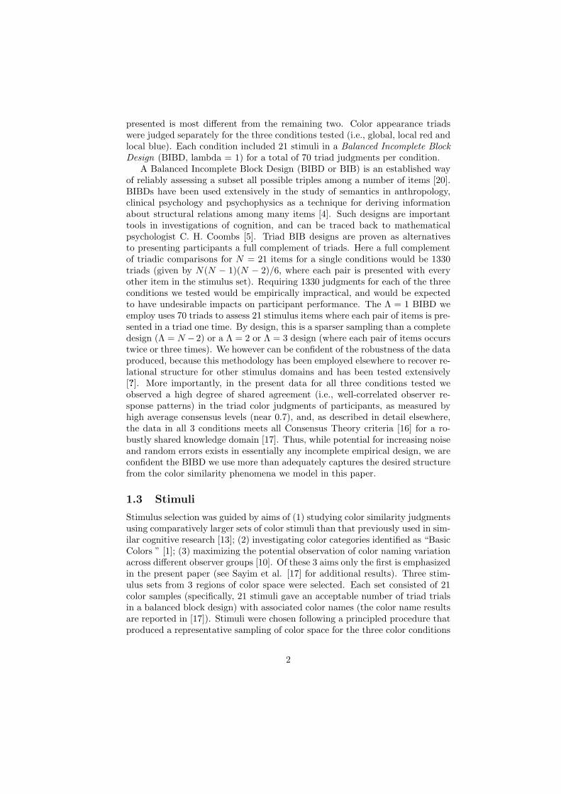
troids identified earlier as corresponding to eight salient color terms [3]. Theremaining 13 global color stimuli corresponded to OSA tiles named with thehighest frequency in a study of unrestricted naming in English of all 424 OSAtiles [6]. Local stimuli were selected to permit comparing similarity structureof within-category conditions with that for global (across-category) stimuli. Bystudying local red and blue color stimuli, we aimed to elicit potential differencesbetween the global and local conditions, following the rationale that color simi-larity judgments should differ for local and global stimulus sets [9]. Red and bluecategories were also chosen to explore a potential difference between observerswith varying color vision capabilities (as aspect of the research presented else-where [17]). A general selection heuristic was used to select red and blue stimuli:the monolexemic naming data of Boynton and Olson[3] was used to identify 21OSA tiles, from each category (red and blue), that were reliably named “red”and “blue” by a majority of their subjects. Minor deviations from this strategywere needed and are described elsewhere [17]. Figure 2 of the main text showsan approximation of the 21 colors sampled for each condition. After triad datacollection subjects answered demographic questions and were screened for colorvision abnormalities. All details of the experimental procedure are found in [17].One triad example from each stimulus condition is shown in figure 1.

Figure 1: Examples of triad stimuli used for the global condition (left), redcondition (middle) and blue condition (right). Colors shown are only approxi-mations of that presented during the experiment on the calibrated color CRTdisplay.

2 Color difference based on distance measure-

ments

2.1 Different distance models

To evaluate the predictions of different color distance models, we use the fol-lowing method. For each condition (global, red, and blue), for each triad wecalculate the three color distances among the three stimuli. The stimulus op-posite the shortest of the distances corresponds to the predicted odd-one-outchoice [2, 15]. For each triad, such theoretically predicted choice is compared to

3

the majority choice of the responders. If the majority of the group picks a stim-ulus different from the predicted one, we call this a “mismatch”. The number ofmismatches (out of the 70 triads for each condition) characterizes roughly howwell a color distance metric alone can predict the observers’ behavior.

Three distance models have been used and indices of color difference:

1. CIELAB. The first distance model [7] is the Euclidean distance measuredby using the three CIELAB coordinates for the two stimuli, L1, a1, b1 andL2, a2, b2:

∆E =√

(L2 − L1)2 + (a2 − a1)2 + (b2 − b1)2.

2. CIE94. The second model we used is the CIE94 delta-E distance formula[8]:

∆E =

√

(L2 − L1)2 +∆C2

(1 + 0.045C)2+

∆H2

(1 + 0.015C)2,

where we defined

C = 1/2

(

√

a21 + b21 +√

a22 + b22

)

,

∆C =√

a22 + b22 −√

a21 + b21, ∆H =√

2(C2 − a1a2 − b1b2).

3. CIEDE2000. Finally, we used the distance defined by the CIEDE2000formula [11] where we employed the implementation algorithm given in[18]. The appropriate formulas are rather lengthy and we refer to the abovesources for the mathematical expressions. CIEDE2000, was recommendedby the CIE in 2001. It includes five corrections to CIELAB: a lightnessweighting function, a chroma weighting function, a hue weighting function,an interactive term between chroma and hue differences for improving theperformance for blue colors, and a factor for re-scaling the CIELAB a*scale for improving the performance for neutral colors[12]. Through suchadjustments some configural visual processing effects, like “crispening”,are addressed. While CIEDE2000 is the newest color difference formularecommended by the Commission International de l’Eclairage, it is nota comprehensive color appearance model, similar to CIELAB and CIE94,but it is by far the most parsimonious and it provides color difference mea-sures that have been empirically shown to be statistically similar (withinsuggested levels of STRESS ≤ 5.0 [?]) to the most recently developedCIECAM02 family of color appearance models (see [19], p. 324 TableXI). We use CIEDE2000 here due to its straightforward, nonparametriccomputational form, and because we considered it a more practical alter-native (i.e., more likely to be used by researchers in color cognition andindustry) to the more advanced CAM models. The latter models strive toincorporate important theoretical parameters, but they still remain com-putationally onerous and untested with respect to their appropriateness asmetrics for cognitive science research on color behaviors or color similarity.

4

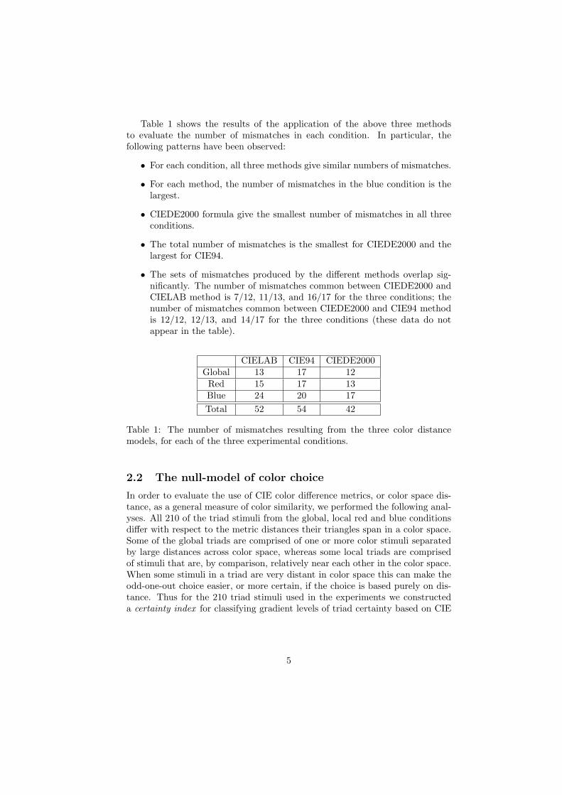
Table 1 shows the results of the application of the above three methodsto evaluate the number of mismatches in each condition. In particular, thefollowing patterns have been observed:

• For each condition, all three methods give similar numbers of mismatches.

• For each method, the number of mismatches in the blue condition is thelargest.

• CIEDE2000 formula give the smallest number of mismatches in all threeconditions.

• The total number of mismatches is the smallest for CIEDE2000 and thelargest for CIE94.

• The sets of mismatches produced by the different methods overlap sig-nificantly. The number of mismatches common between CIEDE2000 andCIELAB method is 7/12, 11/13, and 16/17 for the three conditions; thenumber of mismatches common between CIEDE2000 and CIE94 methodis 12/12, 12/13, and 14/17 for the three conditions (these data do notappear in the table).

CIELAB CIE94 CIEDE2000Global 13 17 12Red 15 17 13Blue 24 20 17

Total 52 54 42

Table 1: The number of mismatches resulting from the three color distancemodels, for each of the three experimental conditions.

2.2 The null-model of color choice

In order to evaluate the use of CIE color difference metrics, or color space dis-tance, as a general measure of color similarity, we performed the following anal-yses. All 210 of the triad stimuli from the global, local red and blue conditionsdiffer with respect to the metric distances their triangles span in a color space.Some of the global triads are comprised of one or more color stimuli separatedby large distances across color space, whereas some local triads are comprisedof stimuli that are, by comparison, relatively near each other in the color space.When some stimuli in a triad are very distant in color space this can make theodd-one-out choice easier, or more certain, if the choice is based purely on dis-tance. Thus for the 210 triad stimuli used in the experiments we constructeda certainty index for classifying gradient levels of triad certainty based on CIE

5

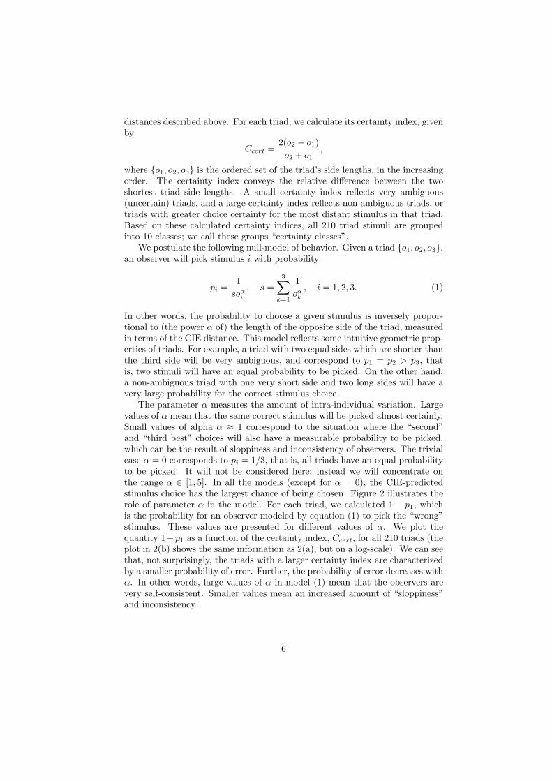
distances described above. For each triad, we calculate its certainty index, givenby

Ccert =2(o2 − o1)

o2 + o1,

where {o1, o2, o3} is the ordered set of the triad’s side lengths, in the increasingorder. The certainty index conveys the relative difference between the twoshortest triad side lengths. A small certainty index reflects very ambiguous(uncertain) triads, and a large certainty index reflects non-ambiguous triads, ortriads with greater choice certainty for the most distant stimulus in that triad.Based on these calculated certainty indices, all 210 triad stimuli are groupedinto 10 classes; we call these groups “certainty classes”.

We postulate the following null-model of behavior. Given a triad {o1, o2, o3},an observer will pick stimulus i with probability

pi =1

soαi, s =

3∑

k=1

1

oαk, i = 1, 2, 3. (1)

In other words, the probability to choose a given stimulus is inversely propor-tional to (the power α of) the length of the opposite side of the triad, measuredin terms of the CIE distance. This model reflects some intuitive geometric prop-erties of triads. For example, a triad with two equal sides which are shorter thanthe third side will be very ambiguous, and correspond to p1 = p2 > p3, thatis, two stimuli will have an equal probability to be picked. On the other hand,a non-ambiguous triad with one very short side and two long sides will have avery large probability for the correct stimulus choice.

The parameter α measures the amount of intra-individual variation. Largevalues of α mean that the same correct stimulus will be picked almost certainly.Small values of alpha α ≈ 1 correspond to the situation where the “second”and “third best” choices will also have a measurable probability to be picked,which can be the result of sloppiness and inconsistency of observers. The trivialcase α = 0 corresponds to pi = 1/3, that is, all triads have an equal probabilityto be picked. It will not be considered here; instead we will concentrate onthe range α ∈ [1, 5]. In all the models (except for α = 0), the CIE-predictedstimulus choice has the largest chance of being chosen. Figure 2 illustrates therole of parameter α in the model. For each triad, we calculated 1 − p1, whichis the probability for an observer modeled by equation (1) to pick the “wrong”stimulus. These values are presented for different values of α. We plot thequantity 1−p1 as a function of the certainty index, Ccert, for all 210 triads (theplot in 2(b) shows the same information as 2(a), but on a log-scale). We can seethat, not surprisingly, the triads with a larger certainty index are characterizedby a smaller probability of error. Further, the probability of error decreases withα. In other words, large values of α in model (1) mean that the observers arevery self-consistent. Smaller values mean an increased amount of “sloppiness”and inconsistency.

6

0.0 0.5 1.0 1.5

10- 4

0.001

0.01

0.1

0.0 0.5 1.0 1.5

0.0

0.1

0.2

0.3

0.4

0.5

0.6

Certainty index Certainty index

Pro

babi

lity

of a

mis

mat

ch

Pro

babi

lity

of a

mis

mat

ch

α=5α=0,...,5

α=0

α=1

α=2

(b)(a)

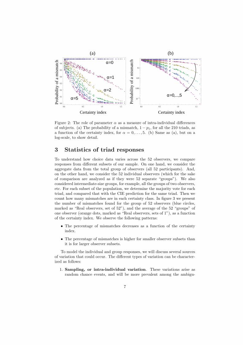
Figure 2: The role of parameter α as a measure of intra-individual differencesof subjects. (a) The probability of a mismatch, 1− p1, for all the 210 triads, asa function of the certainty index, for α = 0, . . . , 5. (b) Same as (a), but on alog-scale, to show detail.

3 Statistics of triad responses

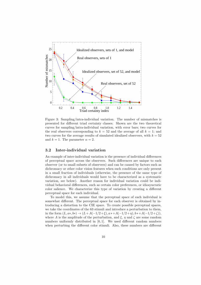
To understand how choice data varies across the 52 observers, we compareresponses from different subsets of our sample. On one hand, we consider theaggregate data from the total group of observers (all 52 participants). And,on the other hand, we consider the 52 individual observers (which for the sakeof comparison are analyzed as if they were 52 separate “groups”). We alsoconsidered intermediate-size groups, for example, all the groups of two observers,etc. For each subset of the population, we determine the majority vote for eachtriad, and compared that with the CIE prediction for the same triad. Then wecount how many mismatches are in each certainty class. In figure 3 we presentthe number of mismatches found for the group of 52 observers (blue circles,marked as “Real observers, set of 52”), and the average of the 52 “groups” ofone observer (orange dots, marked as “Real observers, sets of 1”), as a functionof the certainty index. We observe the following patterns:

• The percentage of mismatches decreases as a function of the certaintyindex.

• The percentage of mismatches is higher for smaller observer subsets thanit is for larger observer subsets.

To model the individual and group responses, we will discuss several sourcesof variation that could occur. The different types of variation can be character-ized as follows:

1. Sampling, or intra-individual variation. These variations arise asrandom chance events, and will be more prevalent among the ambigu-

7

ous triads. These variations are reflected in observer test-retest incon-sistencies, can be ascribed to individual behavior, such as sloppiness incompleting the triad test.

2. Inter-individual variation. These variations reflect (a) inhomogeneitiesof the observers (the presence of a small number of dichromat or anomaloustrichromat observers), or (b) individual cognitive factors such as personalcolor salience or preference.

3. Systematic variation. These variations can arise (a) from inconsisten-cies of the CIE description of the perceptual space, or (b) from somesystematic cognitive factors such as conventions. These variations reflectdeviations from the CIE prediction which are common among a large por-tion of the population.

The three classes of variation listed above have very distinct features, and inthe following sections we discuss their mathematical properties. We show thatvariations of type (1) and (2) alone cannot explain the observed variation, andone must assume the existence of some systematic source of variation, (3).

3.1 Sampling and intra-individual variation

To consider this type of variation in isolation, we assume that all individualshave exactly the same perceptual ordering of stimuli across color space, andthis space is correctly described by a CIE model of color distance. We will notinclude any personal preference or individual differences in the description atthis stage. The observers described here can be called “idealized observers”,because they are identical to each other, and because their perceptual space isdescribed accurately by a CIE color distance formula together with our model(1).

Given this behavioral model, it is obvious that even with a population ofidentical observers, there is a possibility of mismatches, which is larger forsmaller values of α, see previous section. Even though for each individual andfor each triad, there is a stimulus that will most likely be picked, there is stilla probability of picking a suboptimal stimulus. The amount of this effect isincorporated in the parameter α.

For a given value of α in formula (1), we can calculate the probability thatthe majority of the population will pick the CIE-predicted stimulus. Let ussuppose that there are k people in the subset, and defined the quantity k(1/3)

to be the smallest integer such that k(1/3) ≥ k/3. Then the probability for themajority to pick the CIE-predicted stimulus is given by

P1 =k

∑

i1=k(1/3)

i1∑

i2=k−2i1

k!

i1!i2!(k − i1 − i2)!pi11 pi22 pk−i1−i2

3 . (2)

In derivation of this expression we used a non-strict definition of majority: ifthe number of people choosing stimulus i is given by ki with

∑3i=1 ki = k, then

8

ki is a majority if kj ≤ ki with j 6= i.1 In the above formula we assume formallythat the factorial of negative integers is infinite. Under this assumption we seethat with k = 1, we simply have P1 = p1.

Let us suppose that a given certainty class contains m triads. Our theorypredicts how many mismatches we can expect in a population of k idealizedobservers, and the variance of this amount:

E(mis) = (1− P1)m, V ar(mis) = (1− P1)P1m, (3)

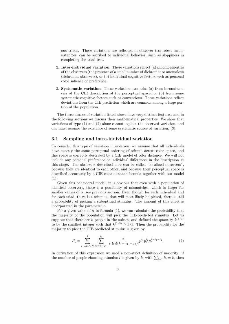
according to the binary distribution.In Figure 3 we illustrate the behavior of the idealized observers. The horizon-

tal axis corresponds to the certainty index, and the vertical axis is the numberof mismatches for each certainty class. The total number of triads in each classcorresponds to our 3 experimental conditions with a total of 210 triads. Figure3’s two curves with error bars are the predictions of our theory with the idealizedobservers. The green curve corresponds to k = 52 observers and the red curveto k = 1 observers. We plot both the expected number of mismatches and thestandard deviation. We can see that the case with k = 52 observers correspondsto a much smaller expected number of mismatches. It is easy to show that ask → ∞, the number of mismatches of the population majority will also tend tozero. This is an inherent property of sampling variation of this kind.

In our model, α is an unknown parameter, which measures the averagedobserver consistency, and which we can choose to make our model match thedata as close as possible. In figure 3 we chose the parameter α = 2 such that thecurve corresponding to the individual real observers lies close to the theoreticalcurve of sampling variation. As we can see however, the curve corresponding tothe group of 52 real observers does not match the sampling variation prediction.Taking different values of α does not improve the situation. The problem is thatin the presence of sampling and intra-individual variation only, the populationof 52 observers performs a lot better (that is, has much fewer mismatches) thanpopulations of 1 observer. That is, the amount of sampling variation decays tozero very fast as the group size increases. This is not the case with the realobservers, whose k = 1 and k = 52 curves are relatively close to each other.From this we can conclude that sampling/intra-individual variation alone donot describe the data completely.

Before we move onto the next type of variation, we point out that in orderto check the validity of formulas (2-3), we have created artificial populations ofidealized observers by picking their triad responses in accordance with proba-bilities pi. The population counts for these observers (in groups of 52 and ingroups of 1, averaged over 20 runs) are also presented in figure 3. They are linesmarked as “Idealized observers, sets of 52” and “Idealized observers, sets of 1”.As expected, both of these lines are in close proximity with the theoreticallypredicted sampling variation lines.

1A strict definition of majority would require a strict inequality.

9

0.2 0.4 0.6 0.8 1.0 1.2 1.4

0

5

10

15

20

25 Idealized observers, sets of 1, and model

Real observers, set of 52

Triad certainty index

Num

ber

of m

ism

atch

es

Idealized observers, set of 52, and model

Real observers, sets of 1

Figure 3: Sampling/intra-individual variation. The number of mismatches ispresented for different triad certainty classes. Shown are the two theoreticalcurves for sampling/intra-individual variation, with error bars; two curves forthe real observers corresponding to k = 52 and the average of all k = 1; andtwo curves for the average results of simulated idealized observers, with k = 52and k = 1. The parameter α = 2.

3.2 Inter-individual variation

An example of inter-individual variation is the presence of individual differencesof perceptual space across the observers. Such differences are unique to eachobserver (or to small subsets of observers) and can be caused by factors such asdichromacy or other color vision features when such conditions are only presentin a small fraction of individuals (otherwise, the presence of the same type ofdichromacy in all individuals would have to be characterized as a systematicvariation, see below). Another reason for individual variation could be indi-vidual behavioral differences, such as certain color preferences, or idiosyncraticcolor salience. We characterize this type of variation by creating a differentperceptual space for each individual.

To model this, we assume that the perceptual space of each individual issomewhat different. The perceptual space for each observer is obtained by in-troducing a distortion to the CIE space. To create possible perceptual spaces,we take the coordinates of the 63 stimuli and introduce a perturbation to them,in the form (L, a∗, b∗) → (L+A(−1/2+ξ), a∗+A(−1/2+η), b∗+A(−1/2+ζ)),where A is the amplitude of the perturbation, and ξ, η and ζ are some randomnumbers uniformly distributed in [0, 1]. We used different random numberswhen perturbing the different color stimuli. Also, these numbers are different

10

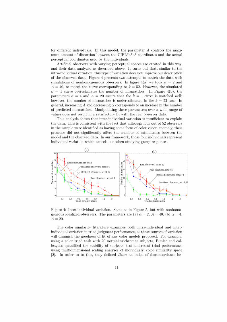
for different individuals. In this model, the parameter A controls the maxi-mum amount of distortion between the CIEL*a*b* coordinates and the actualperceptual coordinates used by the individuals.

Artificial observers with varying perceptual spaces are created in this way,and their data analyzed as described above. It turns out that, similar to theintra-individual variation, this type of variation does not improve our descriptionof the observed data. Figure 4 presents two attempts to match the data withsimulations of nonhomogeneous observers. In figure 4(a) we took α = 2 andA = 40, to match the curve corresponding to k = 52. However, the simulatedk = 1 curve overestimates the number of mismatches. In Figure 4(b), theparameters α = 4 and A = 20 assure that the k = 1 curve is matched well;however, the number of mismatches is underestimated in the k = 52 case. Ingeneral, increasing A and decreasing α corresponds to an increase in the numberof predicted mismatches. Manipulating these parameters over a wide range ofvalues does not result in a satisfactory fit with the real observer data.

This analysis shows that inter-individual variation is insufficient to explainthe data. This is consistent with the fact that although four out of 52 observersin the sample were identified as having some form of color vision anomaly, theirpresence did not significantly affect the number of mismatches between themodel and the observed data. In our framework, those four individuals representindividual variation which cancels out when studying group responses.

0.2 0.4 0.6 0.8 1.0 1.2 1.4

0

5

10

15

20

25

30


Num

ber

of m

ism

atch

es



Idealized observers, set of 52

Idealized observers, sets of 1

(a)

0.2 0.4 0.6 0.8 1.0 1.2 1.4

0

5

10

15

20


Num

ber

of m

ism

atch

es





(b)

Figure 4: Inter-individual variation. Same as in Figure 5, but with nonhomo-geneous idealized observers. The parameters are (a) α = 2, A = 40; (b) α = 4,A = 20.

The color similarity literature examines both intra-individual and inter-individual variation in triad judgment performance, as these sources of variationwill diminish the goodness of fit of any color models proposed. For example,using a color triad task with 20 normal trichromat subjects, Bimler and col-leagues quantified the stability of subjects’ test-and-retest triad performanceusing multidimensional scaling analyses of individuals’ color similarity space[2]. In order to to this, they defined Dmn an index of disconcordance be-

11

tween test (m) and retest (n) datasets for each individual (simply, Dmn is thestraight-line distance between points, as described p. 74 of [2]). They foundthe average within-subject index was Dmn = 0.26, which is an indication of theaverage intra-individual variation in triad similarity scalings across repeatedobservations. By comparison, the average value of Dmn inter-individual vari-ation (between subject variation) overall was Dmn = 0.33. They report thisintra-individual variation to be significantly smaller (p < .05) than the inter-individual variation in color triad similarity structures ([2], p. 74).

The important point for the present paper is that while intra- and inter-individual differences in color similarity structures produced by triad perfor-mance are significantly different, they have similar orders of magnitude (seealso [13]), and the intra-individual differences are smaller (albeit only slightly)than the inter-individual differences. Our experiments did not assess individ-ual repeated observations, so we cannot directly quantify the impact of intra-individual variation on the degree to which our model fits the group data. How-ever, as mentioned earlier in Section 1.2, in all three conditions we investigated,a high degree of shared agreement was seen across participants in triad colorjudgments (using Consensus Theory analyses)[16]. This provides confidencethat the datasets modeled here have, as shown by an independent analysis[17],a high degree of consistency both within and across participants.

In our model, we propose a quantitative way to model the different sourcesof variation. We use the parameter α which is an alternative way to measurethe consistency of observer responses. This measure is in a sense more univer-sal because it allows to compare the consistency of responses across differenttriads, which may differ in their certainty index. To model inter-individualvariations, we vary the underlying individual models of color distances of indi-viduals. We find that inter-individual variations, like intra-individual variations,are not enough to explain the observed responses.

3.3 Systematic variation

An example of systematic variation could arise from inconsistencies in theCIEL*a*b*, CIE-delta E, or CIEDE2000 descriptions of perceptual space, orcognitive behavior patterns common to all the observers that are not includedin the CIE models, such as common conventions. To model this kind of vari-ation, we again assume that all the agents have identical perceptual space (ahomogeneous group of observers), and that it is not necessarily well describedby the CIE formalisms.

To model this situation we assume that the perceptual space (shared byall the observers) is different from the CIE space that we use to identify theCIE-predicted triads. This is done exactly as described in section ??, exceptwe create only one perceptual space, different from CIE and common for allindividuals. To clarify, the difference between the CIEL*a*b* space and theperceptual space could be due to the inconsistencies inherent in the CIE model,or to cognitive factors common to all the observers.

12

0.2 0.4 0.6 0.8 1.0 1.2 1.4

0

5

10

15

20

25


Num

ber

of m

ism

atch

es





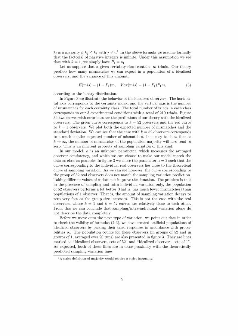
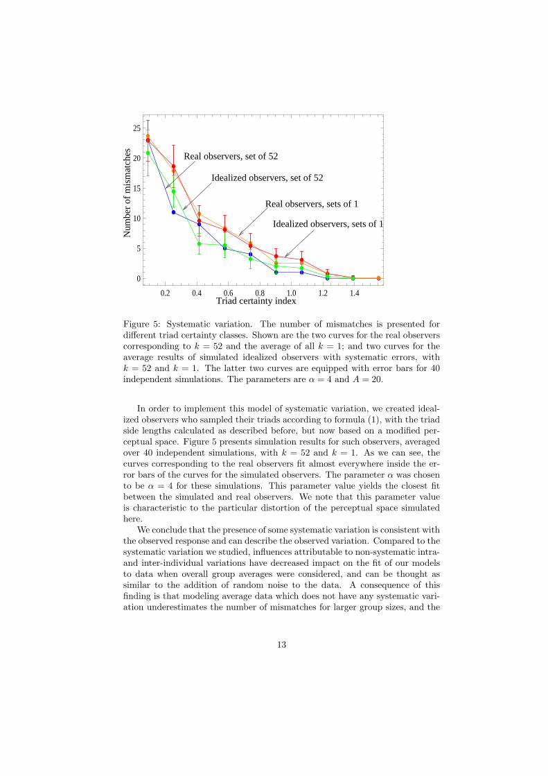
Figure 5: Systematic variation. The number of mismatches is presented fordifferent triad certainty classes. Shown are the two curves for the real observerscorresponding to k = 52 and the average of all k = 1; and two curves for theaverage results of simulated idealized observers with systematic errors, withk = 52 and k = 1. The latter two curves are equipped with error bars for 40independent simulations. The parameters are α = 4 and A = 20.

In order to implement this model of systematic variation, we created ideal-ized observers who sampled their triads according to formula (1), with the triadside lengths calculated as described before, but now based on a modified per-ceptual space. Figure 5 presents simulation results for such observers, averagedover 40 independent simulations, with k = 52 and k = 1. As we can see, thecurves corresponding to the real observers fit almost everywhere inside the er-ror bars of the curves for the simulated observers. The parameter α was chosento be α = 4 for these simulations. This parameter value yields the closest fitbetween the simulated and real observers. We note that this parameter valueis characteristic to the particular distortion of the perceptual space simulatedhere.

We conclude that the presence of some systematic variation is consistent withthe observed response and can describe the observed variation. Compared to thesystematic variation we studied, influences attributable to non-systematic intra-and inter-individual variations have decreased impact on the fit of our modelsto data when overall group averages were considered, and can be thought assimilar to the addition of random noise to the data. A consequence of thisfinding is that modeling average data which does not have any systematic vari-ation underestimates the number of mismatches for larger group sizes, and the

13

underestimation grows as group size increases.

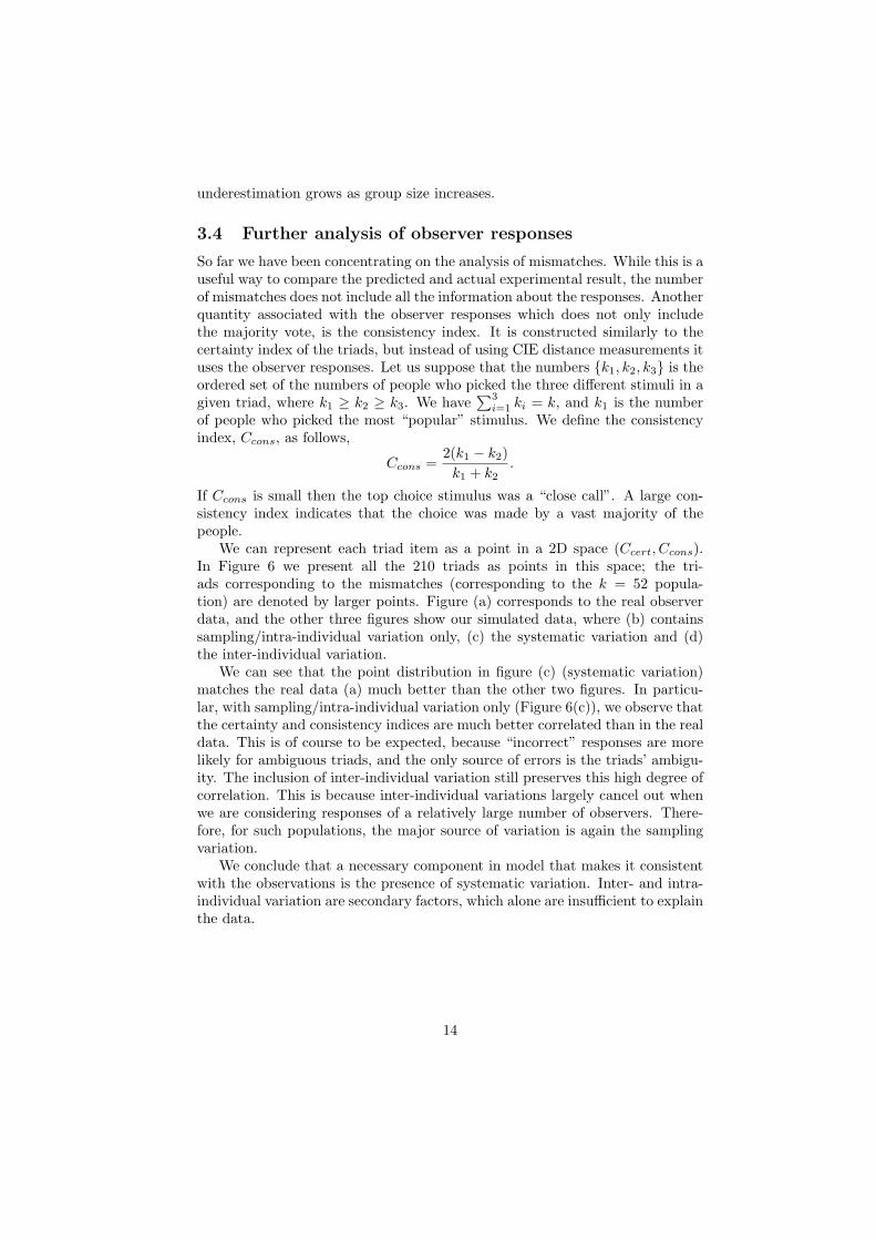
3.4 Further analysis of observer responses

So far we have been concentrating on the analysis of mismatches. While this is auseful way to compare the predicted and actual experimental result, the numberof mismatches does not include all the information about the responses. Anotherquantity associated with the observer responses which does not only includethe majority vote, is the consistency index. It is constructed similarly to thecertainty index of the triads, but instead of using CIE distance measurements ituses the observer responses. Let us suppose that the numbers {k1, k2, k3} is theordered set of the numbers of people who picked the three different stimuli in agiven triad, where k1 ≥ k2 ≥ k3. We have

∑3i=1 ki = k, and k1 is the number

of people who picked the most “popular” stimulus. We define the consistencyindex, Ccons, as follows,

Ccons =2(k1 − k2)

k1 + k2.

If Ccons is small then the top choice stimulus was a “close call”. A large con-sistency index indicates that the choice was made by a vast majority of thepeople.

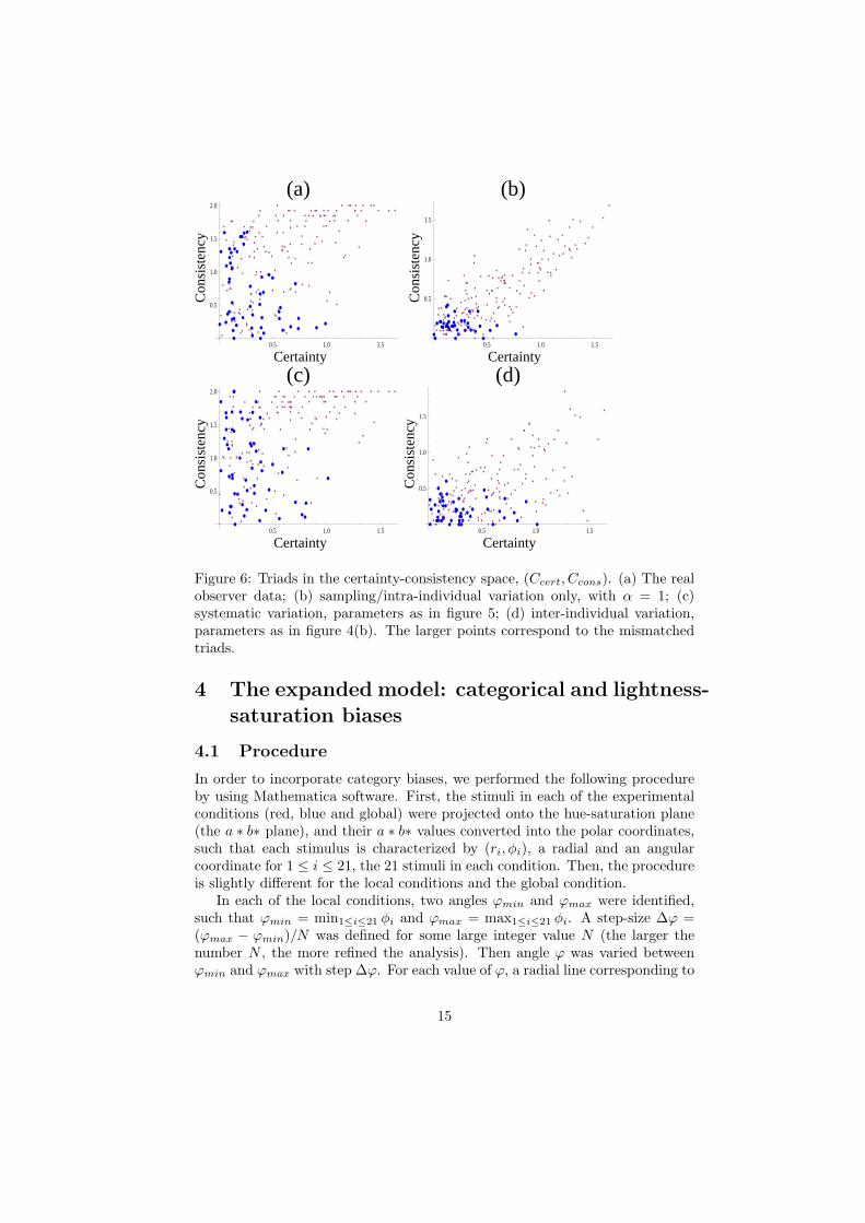
We can represent each triad item as a point in a 2D space (Ccert, Ccons).In Figure 6 we present all the 210 triads as points in this space; the tri-ads corresponding to the mismatches (corresponding to the k = 52 popula-tion) are denoted by larger points. Figure (a) corresponds to the real observerdata, and the other three figures show our simulated data, where (b) containssampling/intra-individual variation only, (c) the systematic variation and (d)the inter-individual variation.

We can see that the point distribution in figure (c) (systematic variation)matches the real data (a) much better than the other two figures. In particu-lar, with sampling/intra-individual variation only (Figure 6(c)), we observe thatthe certainty and consistency indices are much better correlated than in the realdata. This is of course to be expected, because “incorrect” responses are morelikely for ambiguous triads, and the only source of errors is the triads’ ambigu-ity. The inclusion of inter-individual variation still preserves this high degree ofcorrelation. This is because inter-individual variations largely cancel out whenwe are considering responses of a relatively large number of observers. There-fore, for such populations, the major source of variation is again the samplingvariation.

We conclude that a necessary component in model that makes it consistentwith the observations is the presence of systematic variation. Inter- and intra-individual variation are secondary factors, which alone are insufficient to explainthe data.

14

0.5 1.0 1.5

0.5

1.0

1.5

2.0

(a)C

onsi

sten

cy

Certainty0.5 1.0 1.5

0.5

1.0

1.5

0.5 1.0 1.5

0.5

1.0

1.5

2.0

0.5 1.0 1.5

0.5

1.0

1.5

(d)

Con

sist

ency

Certainty

(b)

Con

sist

ency

Certainty

(c)

Con

sist

ency

Certainty

Figure 6: Triads in the certainty-consistency space, (Ccert, Ccons). (a) The realobserver data; (b) sampling/intra-individual variation only, with α = 1; (c)systematic variation, parameters as in figure 5; (d) inter-individual variation,parameters as in figure 4(b). The larger points correspond to the mismatchedtriads.

4 The expanded model: categorical and lightness-

saturation biases

4.1 Procedure

In order to incorporate category biases, we performed the following procedureby using Mathematica software. First, the stimuli in each of the experimentalconditions (red, blue and global) were projected onto the hue-saturation plane(the a ∗ b∗ plane), and their a ∗ b∗ values converted into the polar coordinates,such that each stimulus is characterized by (ri, φi), a radial and an angularcoordinate for 1 ≤ i ≤ 21, the 21 stimuli in each condition. Then, the procedureis slightly different for the local conditions and the global condition.

In each of the local conditions, two angles ϕmin and ϕmax were identified,such that ϕmin = min1≤i≤21 φi and ϕmax = max1≤i≤21 φi. A step-size ∆ϕ =(ϕmax − ϕmin)/N was defined for some large integer value N (the larger thenumber N , the more refined the analysis). Then angle ϕ was varied betweenϕmin and ϕmax with step ∆ϕ. For each value of ϕ, a radial line corresponding to

15

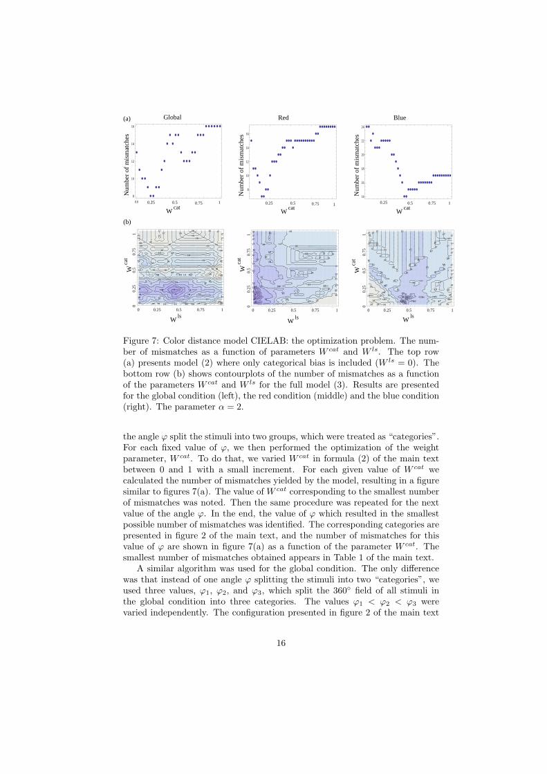
ææ

æ

æ

æææ

æææææ

ææ

æ

æ

æ

æ

ææ

æææææ

æææææææ

æææææææææ

10 20 30 40

14

16

18

20

22

24

æ

æ

æ æ

æ

æ æ

æ æ

æ

æ

æ

æ

æ

æ æ

æ

æ æ æ

æ æ

æ æ æ

æ æ æ æ æ æ

0.0 0.2 0.4 0.6 0.8 1.0

8

10

12

14

16

æ

ææ

æ

æ

ææ

ææ

æ

æææ

ææ

ææ

æææ

æ

ææææææææææ

ææ

ææææææææ

10 20 30 40

8

10

12

14

16

78

91010

1112

12

15

15

15

15

15

15

17

17

17

17

17

17

17

19

19

19

19

19

19

19

19

21

21

21

21

2121

21

21

21

21

21 21

21

2323

23

25

25

25

25

5 10 15 20

10

20

30

40

910

10

11

11

12

1212

12

15

15

15

15

15

15

15

15

15

15

151515

15 1515

15 15

17

17

17

17

17

17

17

17

17

17 1717

17

17

17 1717

17

1717

17

17

1717

17

17

17

1717

17

17

1717

19

19

19

19

19

21 21

21

21

21

21

21

21

21

23

5 10 15 20

10

20

30

40

6

7

8 8

9

9

10

10

10

11

11

11

12

12

12

12

13 13 13

13

13

13

13

14 14 14 14

14

14

14 14 14 14

1414

14

1515

1515

15

15

15

16

16

16

16

1616

1616

16

1616

16

16

16

16

16

17

17

17

17

17

17

1717

17

18

18

5 10 15 20

5

10

15

20

25

30

Wca

t

Wca

t

Wca

t

Wls

Wls

Wls

0 0.25 0.5 0.75 1

10.

250

0.75

0.5

Wcat

Num

ber

of m

ism

atch

es

Red

Wcat

Num

ber

of m

ism

atch

es

0 0.25 0.5 0.75 1

10.

250

0.75

0.5

Blue

Wcat

Num

ber

of m

ism

atch

es

0 0.25 0.5 0.75 1

10.

250

0.75

0.5

(b)

(a) Global

0.25 0.5 0.75 1 0.25 0.5 0.75 1 0.25 0.5 0.75 1

Figure 7: Color distance model CIELAB: the optimization problem. The num-ber of mismatches as a function of parameters W cat and W ls. The top row(a) presents model (2) where only categorical bias is included (W ls = 0). Thebottom row (b) shows contourplots of the number of mismatches as a functionof the parameters W cat and W ls for the full model (3). Results are presentedfor the global condition (left), the red condition (middle) and the blue condition(right). The parameter α = 2.

the angle ϕ split the stimuli into two groups, which were treated as “categories”.For each fixed value of ϕ, we then performed the optimization of the weightparameter, W cat. To do that, we varied W cat in formula (2) of the main textbetween 0 and 1 with a small increment. For each given value of W cat wecalculated the number of mismatches yielded by the model, resulting in a figuresimilar to figures 7(a). The value of W cat corresponding to the smallest numberof mismatches was noted. Then the same procedure was repeated for the nextvalue of the angle ϕ. In the end, the value of ϕ which resulted in the smallestpossible number of mismatches was identified. The corresponding categories arepresented in figure 2 of the main text, and the number of mismatches for thisvalue of ϕ are shown in figure 7(a) as a function of the parameter W cat. Thesmallest number of mismatches obtained appears in Table 1 of the main text.

A similar algorithm was used for the global condition. The only differencewas that instead of one angle ϕ splitting the stimuli into two “categories”, weused three values, ϕ1, ϕ2, and ϕ3, which split the 360◦ field of all stimuli inthe global condition into three categories. The values ϕ1 < ϕ2 < ϕ3 werevaried independently. The configuration presented in figure 2 of the main text

16

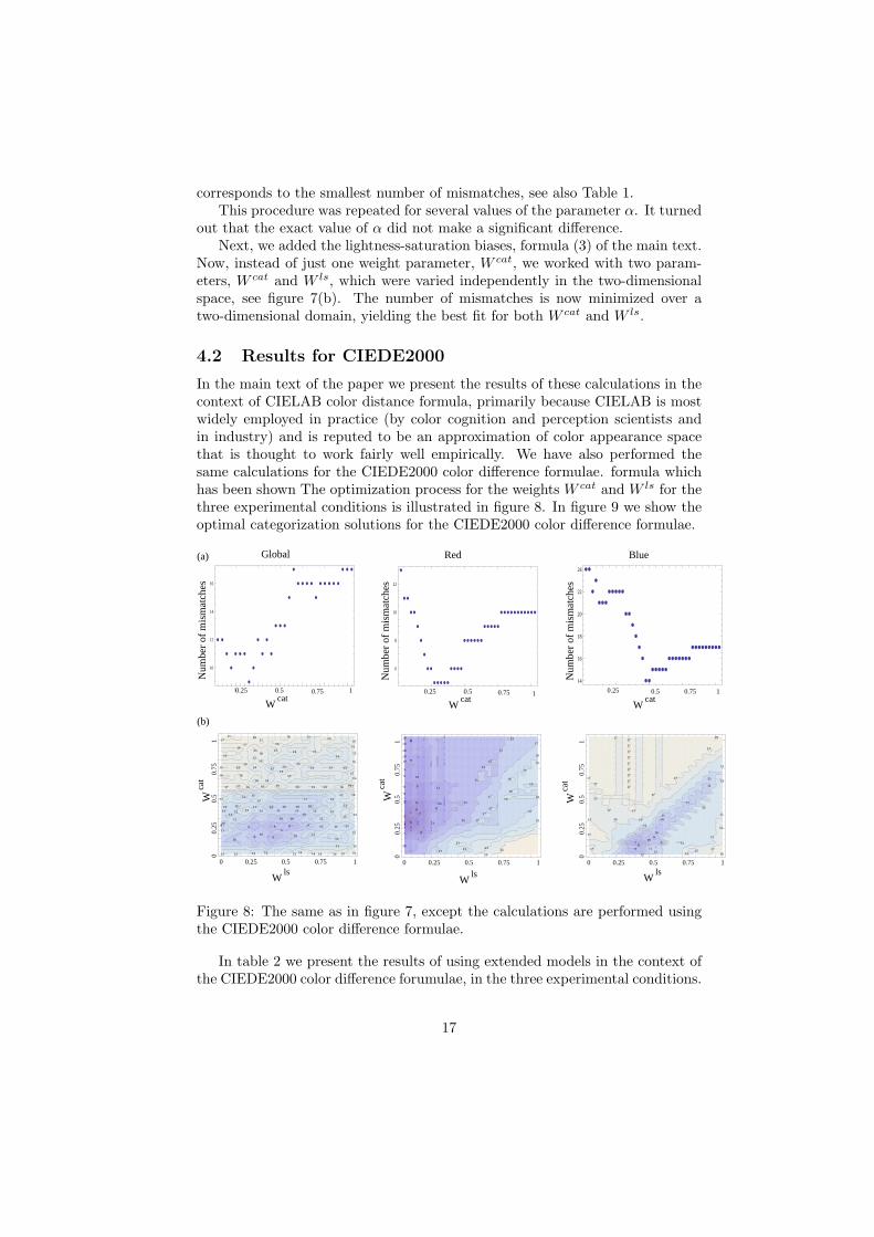
corresponds to the smallest number of mismatches, see also Table 1.This procedure was repeated for several values of the parameter α. It turned

out that the exact value of α did not make a significant difference.Next, we added the lightness-saturation biases, formula (3) of the main text.

Now, instead of just one weight parameter, W cat, we worked with two param-eters, W cat and W ls, which were varied independently in the two-dimensionalspace, see figure 7(b). The number of mismatches is now minimized over atwo-dimensional domain, yielding the best fit for both W cat and W ls.

4.2 Results for CIEDE2000

In the main text of the paper we present the results of these calculations in thecontext of CIELAB color distance formula, primarily because CIELAB is mostwidely employed in practice (by color cognition and perception scientists andin industry) and is reputed to be an approximation of color appearance spacethat is thought to work fairly well empirically. We have also performed thesame calculations for the CIEDE2000 color difference formulae. formula whichhas been shown The optimization process for the weights W cat and W ls for thethree experimental conditions is illustrated in figure 8. In figure 9 we show theoptimal categorization solutions for the CIEDE2000 color difference formulae.

ææ

æ

æ

æææ

æææææ

ææ

æ

æ

æ

æ

ææ

æææææ

æææææææ

æææææææææ

10 20 30 40

14

16

18

20

22

24

æ æ

æ

æ

æ æ æ

æ

æ

æ

æ

æ

æ

æ æ æ

æ

æ

æ æ æ æ

æ

æ æ æ æ æ

æ æ æ

5 10 15 20 25 30

10

12

14

16

æ

ææ

ææ

æ

æ

æ

ææ

æææææ

ææææ

ææææææ

æææææ

æææææææææææ

10 20 30 40

6

8

10

12

5

5

6

6

7

7

8

8

8

8

8

9

9

9

10

10

10

10

10

10

10

10

11

11

11

11

11

12

15

15

15

15

15

15

17

17

17

17

17

17

19

1919

19

19

19

19

19

19

21

21

21

23

25

25

5 10 15 20

10

20

30

40

78

9

9

910

10

1011

11

11

11

11

12

12

12

12

1212

12

15

15

15

15

15

15

15

17 17

17

17

17

17

17 17

17

17

1717

17

17

17

17

17

17

1717

17

17

19

19

5 10 15 20

10

20

30

40

8 89

9

9 9

99

10

10

10

1010

10

10 10

10 10 10 10

11

11

11

11

11 11

1111 11

11 11

11

12 12 12 12

12

12

12

12 12

12 12 12

12

12 12

13

13

13

13

13

13 13

13

1313 13 13 13

14 14 14 14

14

14

14

14

14

1414

14

15

15

15

15

15

15

15

15

15

15 15 15

15

15 1515

15

15

16

1616

161616

16

16

16

1616

16

1616

16 16 16

16

16

1717

17

1717

17

17

5 10 15 20

5

10

15

20

25

30

Wca

t

Wca

t

Wca

t

Wls

Wls

Wls

Wcat

Num

ber

of m

ism

atch

es

Red

Wcat

Num

ber

of m

ism

atch

es

0 0.25 0.5 0.75 1

10.

250

0.75

0.5

Blue

Wcat

Num

ber

of m

ism

atch

es

0 0.25 0.5 0.75 1

10.

250

0.75

0.5

(b)

(a) Global

0.25 0.5 0.75 1 0.25 0.5 0.75 1 0.25 0.5 0.75 1

0 0.25 0.5 0.75 1

10.

250

0.75

0.5

Figure 8: The same as in figure 7, except the calculations are performed usingthe CIEDE2000 color difference formulae.

In table 2 we present the results of using extended models in the context ofthe CIEDE2000 color difference forumulae, in the three experimental conditions.

17

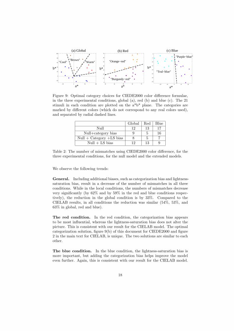
30 40 50 60 700

10

20

30

40

50

60

70

-50 0 50 100

-20

0

20

40

60

80

100

-20 -10 0 10 20

-35

-30

-25

-20

-15

-10

-5

0

a*

b*

(a) Global (b) Red (c) Blue

a*

b*

a*

b*

"Orange−red"

"Burgundy−red"

"Purple−blue"

"Teal−blue"

"Warm""Brown"

"Cool"

Figure 9: Optimal category choices for CIEDE2000 color difference formulae,in the three experimental conditions, global (a), red (b) and blue (c). The 21stimuli in each condition are plotted on the a*b* plane. The categories aremarked by different colors (which do not correspond to any real colors used),and separated by radial dashed lines.

Global Red BlueNull 12 13 17

Null+category bias 9 5 16Null + Category +LS bias 8 5 7

Null + LS bias 12 13 9

Table 2: The number of mismatches using CIEDE2000 color difference, for thethree experimental conditions, for the null model and the extended models.

We observe the following trends:

General. Including additional biases, such as categorization bias and lightness-saturation bias, result in a decrease of the number of mismatches in all threeconditions. While in the local conditions, the numbers of mismatches decreasevery significantly (by 62% and by 59% in the red and blue conditions respec-tively), the reduction in the global condition is by 33%. Compared to theCIELAB results, in all conditions the reduction was similar (54%, 53%, and63% in global, red and blue).

The red condition. In the red condition, the categorization bias appearsto be most influential, whereas the lightness-saturation bias does not alter thepicture. This is consistent with our result for the CIELAB model. The optimalcategorization solution, figure 9(b) of this document for CIEDE2000 and figure2 in the main text for CIELAB, is unique. The two solutions are similar to eachother.

The blue condition. In the blue condition, the lightness-saturation bias ismore important, but adding the categorization bias helps improve the modeleven further. Again, this is consistent with our result for the CIELAB model.

18

The optimal categorization for CIELAB (figure 2 of the main text) is unique,and the optimal categorization for CIEDE2000 (figure 9(c) of this document)consists of three very similar ways of splitting the colors, all very similar to theone depicted in figure figure 9(c).

The global condition. In the global condition, both categorization andlightness-saturation biases appear to play a role. The power of the modifiedmodel, however, is more significant when used in combination with the CIELABdistance formula (where it reduces the number of mismatches from 13 to 5), com-pared with the CIEDE2000 formula, where the reduction is less significant (from12 to 8). In the latter case, we observe many different optimal categorizationsolutions, all resulting in 8 mismatches. One of these solutions is shown in figure9(a).

References

[1] Berlin, B., & Kay, P. (1969). Basic color terms: Their universality and

evolution. Berkeley: University of California Press.

[2] Bimler, D., Kirkland, K. & Pichler, S. (2004). Escher in color space:Individual-differences multidimensional scaling of color dissimilarities col-lected with a gestalt formation task. Behavior Research Methods, Instru-ments, & Computers 2004, 36 (1), 69-76

[3] Boynton, R. M. & Olson, C. (1987). Locating basic colors in the OSA space.COLOR Research and Application, 12, 94–105.

[4] Burton, M.L. & S.B. Nerlove. 1976. Balanced Designs for Triads Tests:Two Examples from English. Social Science Research 5, 247–267.

[5] Coombs, C. H. (1964). A Theory of Data. Wiley, New York.

[6] D’Andrade, R. G. (2003). English color naming data for 424 OSA colortiles. Unpublished research report. University of California, San Diego. De-partment of Anthropology.

[7] CIE94: DeCusatis, C. (1997). Handbook of Applied Photometry, Aip PressSeries, Optical Society of America. Springer publishers. Page 370, Eq. 10.54.

[8] CIE94: DeCusatis, C. (1997). Handbook of Applied Photometry, Aip PressSeries, Optical Society of America. Springer publishers. Page 372, Eq. 10.66.

[9] Indow, T. (1988). Multidimensional studies of Munsell color solid. Psycho-logical Review, 95,456-470.

[10] Jameson, K. A., Highnote, S. M., & Wasserman, L. M. (2001). Richer colorexperience in observers with multiple photopigment opsin genes. Psycho-nomic Bulletin & Review, 8, 244-261.

19

[11] Luo, M.R. and Cui, G. and Rigg, B. (2001) The development of the CIE2000 colour-difference formula: CIEDE2000, Color Research & Application26, 340–350.

[12] Luo, M. R. (2006). Colour difference formulae: past, present and future.(pp. 145-150). In the Proceedings of the ISCC/CIE Expert Symposium2006. “75 Years of the CIE Standard Colorimetric Observer”, 16-17 May2006. NRC, Ottawa, Ontario, Canada. Publ. CIE x030:2006.

[13] Moore, C. C., Romney, A. K., & Hsia, T.-L. (2002). Cultural, gender, andindividual differences in perceptual and semantic structures of basic colorsin Chinese and English. Journal of Cognition and Culture, 2, 1–28.

[14] Romney, A. K., Boyd, J. P., Moore, C. C., Batchelder, W. H. & Brazill, T.J. (1996) Proc. Natl. Acad. Sci. USA 93, 4699–4705.

[15] Paramei, G.V. (2005) Singing the Russian blues: An argument for cultur-ally basic color terms. Cross-Cultural Research 39, 10–38.

[16] Romney, A.K., Weller, S.C. & Batchelder, W.H. (1986). Culture as consen-sus: A Theory of culture and informant accuracy. American Anthroplogist99,313-338

[17] Sayim, B., Jameson, K. A., Alvarado, N. and Szeszel, M. K. (2005). Seman-tic and Perceptual Representations of Color: Evidence of a Shared Color–Naming Function. The Journal of Cognition & Culture, 5(3/4), 427–486.

[18] Sharma, G. and Wu, W. and Dalal, E.N. (2005) The CIEDE2000 color-difference formula: Implementation notes, supplementary test data, andmathematical observations, Color Research & Application 30, 21–30.

[19] Wang, H., Cui, G., Luo, M. R., & Xu, H. (2011). Evaluation of colour-difference formulae for different colour-difference magnitudes. Color Re-search and Application, 37(5), 316–325.

[20] Weller, S. C. & Romney, A. K. (1988). Systematic Data Collection. Quali-tative Research Methods, Volume 10. Sage Publications: London.

20

Documents

A quantitative theory of human color choices - Institute for